Merging 6-beam scans
Introduction:
The work from Sathe et al. 2015 introduces an alternative scanning strategy to be used by wind Doppler lidars for estimating turbulence (6-beam). This new strategy consists of measuring the radial wind on five equally spaced azimuths with fixed elevation, different from 0 or 90 degrees, and one additional measurement from the zenith.
This example shows how to use the lidarwind to retrieve wind speed and direction profiles from the 6-beam observations. The profiles are retrieved using the FFT, following the method proposed by Ishwardat 2017.
Steps:
Download data from zenodo
Read the WindCube’s data
Merge data from one hour of observations
Re-structure the data for using the wind retrieval
Retrieve wind speed and directin profiles
Visualisation
[1]:
import matplotlib.pyplot as plt
import lidarwind
from lidarwind.utilities import sample_data
Step 0: Downloading the sample data
Using pooch the sample dataset will be cached in your system.
[2]:
file_list = sample_data("wc_6beam")
Step 1 and 2: reading and merging the 6-beam data
[3]:
file_list = sorted(file_list)
merged_ds = lidarwind.DataOperations(file_list).merged_data
/Users/jdiasneto/Projects/LST_package_name/lidarwind/data_operator.py:147: UserWarning: rename 'range' to 'range90' does not create an index anymore. Try using swap_dims instead or use set_index after rename to create an indexed coordinate.
  self.tmp90 = self.tmp90.rename({var: f"{var}90"})
Below you can see all the variables available on the original WindCube’s data. Not all of them are needed for retrieving the wind profiles. Note that the variables from the vertical observations are kept separate from the slanted observation.
[4]:
merged_ds
[4]:
<xarray.Dataset>
Dimensions:                                  (time: 715, range90: 143,
                                              range: 137)
Coordinates:
  * time                                     (time) datetime64[ns] 2021-05-13...
  * range90                                  (range90) int32 100 150 ... 7200
  * range                                    (range) int32 104 156 ... 7124 7176
Data variables: (12/34)
    scan_file                                (time) object b'(\xe1\x18\xd5\xf...
    settings_file                            (time) object b'E\xc7_t<\xb7\x10...
    res_file                                 (time) object b'7\x1bb\x06\x0f\x...
    ray_angle_resolution                     (time) float64 0.0 0.0 ... 0.0 0.0
    range_gate_length                        (time) float64 50.0 50.0 ... 50.0
    ray_accumulation_time                    (time) float64 2e+03 ... 2e+03
    ...                                       ...
    radial_wind_speed                        (time, range) float64 1.8 ... -3...
    radial_wind_speed_ci                     (time, range) float64 100.0 ... 0.0
    radial_wind_speed_status                 (time, range) float32 1.0 ... 0.0
    doppler_spectrum_width                   (time, range) float64 0.91 ... 2.92
    doppler_spectrum_mean_error              (time, range) float64 2.6 ... 55.7
relative_beta (time, range) float64 1.01e-07 ....- time: 715
- range90: 143
- range: 137
- time(time)datetime64[ns]2021-05-13T12:00:03.719000064 .....
- standard_name :
- time
- comments :
- Number of seconds between time_reference and the end of each ray measurement.
array(['2021-05-13T12:00:03.719000064', '2021-05-13T12:00:08.976000000', '2021-05-13T12:00:14.748000000', ..., '2021-05-13T12:59:47.996000000', '2021-05-13T12:59:53.252000000', '2021-05-13T12:59:58.551000064'], dtype='datetime64[ns]') - range90(range90)int32100 150 200 250 ... 7100 7150 7200
- standard_name :
- projection_range_coordinate
- units :
- m
- long_name :
- range_to_measurement_volume
- comments :
- Distance along the line of sight, between the instrument and the center of each range gate. Either a dimension or a variable. When this vector is a dimension, gate_index is a variable and vice versa.
- axis :
- radial_range_coordinate
- spacing_is_constant :
- true
- meters_to_center_of_first_gate :
- 100
- meters_between_gates :
- 50
array([ 100, 150, 200, 250, 300, 350, 400, 450, 500, 550, 600, 650, 700, 750, 800, 850, 900, 950, 1000, 1050, 1100, 1150, 1200, 1250, 1300, 1350, 1400, 1450, 1500, 1550, 1600, 1650, 1700, 1750, 1800, 1850, 1900, 1950, 2000, 2050, 2100, 2150, 2200, 2250, 2300, 2350, 2400, 2450, 2500, 2550, 2600, 2650, 2700, 2750, 2800, 2850, 2900, 2950, 3000, 3050, 3100, 3150, 3200, 3250, 3300, 3350, 3400, 3450, 3500, 3550, 3600, 3650, 3700, 3750, 3800, 3850, 3900, 3950, 4000, 4050, 4100, 4150, 4200, 4250, 4300, 4350, 4400, 4450, 4500, 4550, 4600, 4650, 4700, 4750, 4800, 4850, 4900, 4950, 5000, 5050, 5100, 5150, 5200, 5250, 5300, 5350, 5400, 5450, 5500, 5550, 5600, 5650, 5700, 5750, 5800, 5850, 5900, 5950, 6000, 6050, 6100, 6150, 6200, 6250, 6300, 6350, 6400, 6450, 6500, 6550, 6600, 6650, 6700, 6750, 6800, 6850, 6900, 6950, 7000, 7050, 7100, 7150, 7200], dtype=int32) - range(range)int32104 156 208 260 ... 7072 7124 7176
- standard_name :
- projection_range_coordinate
- units :
- m
- long_name :
- range_to_measurement_volume
- comments :
- Distance along the line of sight, between the instrument and the center of each range gate. Either a dimension or a variable. When this vector is a dimension, gate_index is a variable and vice versa.
- axis :
- radial_range_coordinate
- spacing_is_constant :
- true
- meters_to_center_of_first_gate :
- 104
- meters_between_gates :
- 52
array([ 104,  156,  208,  260,  312,  364,  416,  468,  520,  572,  624,  676,
        728,  780,  832,  884,  936,  988, 1040, 1092, 1144, 1196, 1248, 1300,
       1352, 1404, 1456, 1508, 1560, 1612, 1664, 1716, 1768, 1820, 1872, 1924,
       1976, 2028, 2080, 2132, 2184, 2236, 2288, 2340, 2392, 2444, 2496, 2548,
       2600, 2652, 2704, 2756, 2808, 2860, 2912, 2964, 3016, 3068, 3120, 3172,
       3224, 3276, 3328, 3380, 3432, 3484, 3536, 3588, 3640, 3692, 3744, 3796,
       3848, 3900, 3952, 4004, 4056, 4108, 4160, 4212, 4264, 4316, 4368, 4420,
       4472, 4524, 4576, 4628, 4680, 4732, 4784, 4836, 4888, 4940, 4992, 5044,
       5096, 5148, 5200, 5252, 5304, 5356, 5408, 5460, 5512, 5564, 5616, 5668,
       5720, 5772, 5824, 5876, 5928, 5980, 6032, 6084, 6136, 6188, 6240, 6292,
       6344, 6396, 6448, 6500, 6552, 6604, 6656, 6708, 6760, 6812, 6864, 6916,
       6968, 7020, 7072, 7124, 7176], dtype=int32)
- scan_file(time)objectb'(\xe1\x18\xd5\xff\xab\xd1\xad\...
- comments :
- Binary content of scan file.
array([b'(\xe1\x18\xd5\xff\xab\xd1\xad\x9cw\x8ft"?+\xe8\xc7\xef?\xf8\xbfv\x99\xef\x90\xd2\x0e\xb5L\x06\x00\x9aU\x8e\xefWG\xad?K[\xe7z\t\xa7\xd0\x9c]~\x8dw[.\xbbS\xc3w\xe0)!wO\xc2}@\xf1\xc1R7V\x19\xbc\xa7\xbe\xeb\x92\x0e\xba\xc3P\x80\x17\xba\x8a%\xac\x07w\xaf\xed\x8e\xf2\'\x89\x86N\x8b\x8b\xa0\xc5\x96\x06\xef:\xd2\xcbmN\x88&LDt(\xab\xe6S\xa6\xcc\xbc\xa9\xda\x13+\x85\xcc\xf6;\x1b\xfd7iR2\xc4zr\xd5\xc7\x04\xd0j\xf8\xb8Af-\xffFUJ\x95F\xf1V\xd7\x19#\x92\x9a\x12\xf6\x9c;H\x8b\x13\xab\xf8m"<\xb4\x99\x9b\xa3\x1f1\xec5\xed?\xa7G\\\xc5\x85\x92&D\x00\xf0\xa2\xf8y\xa6\xa8X\xffs\xbf\xf3\\k#\xab:B\xfc\x0ca\x02\x97\xb5n\xc8\xfd\xe6\xe1\x90\x90\xabG\x93\x0820\x9e\xb6rz\x1b\xd6\xf9a\t\x84\xc6\x1a\xca\xa6\xce\xce\xabq\xa1\xad(\x94\x80\xc1\xce\xde\x1b\x14\x9d[\x12mZ\x1f\xf8\xe1r\n\x07\x95y\xb3\x97\xceQ^\xb1\xd0\x16ui\x06\xc2\x1d\xde\xd8\xb4\xdb\xd0\x04\xd6\xf7`\x07<\xe0.\xdf\t\xe9\xff\x9b\xe8\xbcU\xe9\x9e\xe1\xdb\x05\xee\xc5\x7f\xf1*Z\x8avY\xe2\xc7Q}\x02AAL\x0f\xc9~\xc997\xb8\xc2p\xb86\xba\x0c\x83\xe6\xf4\xbc\xf4\x1c\x00\x9c\xe4H\xf4b\xe1\x15\xf6\xd7\xb9\xceYE\x8b\x1f\x006n\x04b\x12Q|\xe4\xb7\xff\x99\xdfj\xe9\xeb\x86\xa8\x02{\xcc\x83\x01~\tF[\xa3*\\\xe0\'\xb5\xee:\xc4\xc5\xea\xdb\xa63\xa37\xb1\xcf\xb6Z\xdb\x94\xee#\xeb)x\xd1b\xcf9\x05\xa7@\x10q\t\xc3\xc6\x1a\xc9m\xaaN\xde\xcc\x02\x1f0\xe7q\xcfGY\x9aI\xa9\xf6\xfc\xee\x8c\xee\x1c_\x9e\x8bA\x8b\xab\xfa\xda\x99\xcd\xc7!?\xdd\xcf\xf9nmw\x97V\xf6<\xb5\xc6\xcc\x84\xbbzs\n\xf4\xde\xdf7\xc7\xb4\xc27"O\xb3\x13|\xaf\x9afpd=#\x81\xc3\x92\xa8\xd2\xf1#\x0c \xa0\xae\x05\xd5\xb90PT\xa9\x12X\x9aTA\xf5\xea\xc6?\xc6_\xc5G\xc0TI[\x8a\xffK\xe9\xa3\xc2\xc1\x98I\xb9\x90Myv\x85\x91\xe0\x0b\xd7z\xd1l\xde\x8aq\x93\xffV\xa4rah\x96g3\x1b\xef\xd3\t2\xc0\xdc\xf3\x87Q\xdf \xe4\xb8\xd7\x19\xb1\xc2z\x1e\x8f\xc5H\xb8\xaf\xa3g\x8e\xae\xa1\x8e\x1f4\xbe\xcd2\xc0\xf5\x1c\xb7\x9eu\xdc8\x02}\xd6@\x13\x1blp\x7f\xe4\xa7A\xc9\x01~\x87\xf0\xd7\x95\x99\x95\xdd\xe3\xa9\xd2,j\xde\x18\x83|\xb7:\\\xff\x89\xe5dy\xc7\'\xdd\x8d\x98\'\xfa\x00u\xf10{\x88en1\xa2\x15\x88v#\x96"\xbdKPm\xd5\xc8+\xc6\xdd\x04\xc7\x9d\x18Y\xf8\xdc\x06\xc5\xc9\xa6\xbb"%\xaep\x8e\x84 \xab\x92\x9c\xc5\r\xec\xb8\xf8\xb0rYsz\xc1\xcc\xfa\x9b\x17){\xef\xbc\x1e\xd7\xbe1^I{\xf4\xbe\xd5\xbc\x11>a\x90>(\xa5\xd8|\xf6-D^\'\xd0\x1b\xd1\x91H\x81VqonS\xa8d\xe96\x82\xe9\x8b\x05T5\xd2\xb2\x0f\xe7\x1b?,\xbf\xec\xe9\xda\x1c\xb6e\xa4\n\xdd\xd0\xef\xc8hRS\x84Bc]\x12.U\xc7(k\x83%\x94\x7f\x9d\x86v4M\xc5\xc2\x08\x9c\x85\x92\x06\xf4 s~\xba\x81\xe8*\xbd\xfe\xb7\xc6W\x01\xef\n^\x0b\xc0\xf5\x06\x86\x9e\x1c\x86\xc5\xbf\xcb\xbb\xe8\x8b=\xcc\xde\x1a-N1\xe5w\x0b\x1b\x97[6\x08\x8a[\xe7\xfa\x10o\x1a!\xcd\x02)\xec\xee\xbc\xc9\xee\t\x96\xed\x11\x7f\x8b\xbf\xa2\x0b\xe8\xdd\xe4\xd8\tLu\xa7\x1a\x16v\xda\xb3\x8bY\x1euA\x91\xbe\xc3Qt\xc8\xca\xa5\xd9\xbf\tFZ\xbeH{\xf7\x04-q\xae\x82\xe5\xd0\xbc\x00\xc1P\x9e\x0b\x9a\xbd\xa2}\xb0\xd7\xbaT\xdf\xea\xd6\xa9\x02\xc7k\x00\xd4nf~B\x02\xde[\xc1\xc7m=*\xae\x15\xf9\xd1U\xdf\xe4`\xf5\xa9E\xa0\xc5{\xb7>\x8c\xa6\x16SK/\xd5\xf1\xfa\x90FZ8\xb8\x1bQx\xec\x04R1E|g\x08\xa2W\x98\x92]E\x0c \xfd$\xe8\x01\x82\xe1\xa7]C\xf0\x1e`\x7f\x02J\xc1\xda\xcf\x9f\x8e~6\x0c\x02m\xdb\x1e\x0e"\xa24ot\xaa\x9e\xcff#\x17\xe2\xbf\xb4&dn#\xfbZ,\x86\xc8\xbe\x06\xd2\xb8(@\xe0\xeej\xc9G\x16\xdf\xfc4}\xa0\x13@a\x8b\xaa\xf7\xe50\xfb\x1ff\xc6lm:1E\xcc\x8b\xd4\xe1\x15&\xea\xeb\xe6A\x17_\xdb\xb7\xa9\xfc\x84\x1c\xf3\xd0\\\xfb\xb4\xc4\xd5\x9c\x9b\tW\x9e\xa0-\xa5az9\xea\xd1\xee>\xd5\xf49\xd8\xa6\xed\xad[\xf7\xee\xd7\xb8\xe7_\xdby\xbdr;\xaf\x08\x84\xf9K\xb07\xac\x0e8{\n\x98&Fh]\xb0l\xde\xd1 \xa0F\xd5\x9c+L\xe1^\xf44\xb9\xb2q\xc5\x94Ga-\x7f\xfd\x15G\x90B\xcf\xf6\x9a\xcd\xbfp\xd7\x85\xb0@\x0e\x93\t(\x08\xb3\xd7M%\xfdRl\xa4\xb1\xd4R\xc0<\xca\xebG\x9crP\xb1\xa37\x021Z\x04Y}\xb1\xd6\xa5\xcd\x9fG\x84"7\xec(&\xdf\xd6\xd7k\xb2Q\xcekXL\xa4\xb2t\x89rb\xf8P\xb9\xcfu\x8c\xaa\xd2s\xb5\x1fRQ\x02\xb0Hp\x07\xd9\xe5\x8f\xc9\x93o\x12\xcb\x11\xe6\x12\xed\xe5\x8fHY\x7f\xc5[:p);B\xaf\xda\xca\x86\xf9\xfa\xfb\xd27\xa4\xb1`\x17\x8b\xb9\x97\xa8- 8Au\xcd\xee\x91\x1c\xd7\xb7/\xcf%\xf4l\x07\x1b\xc2B;\xcf\x97\xd9\x1f\x0e+\x19\x93\x93\x17\xe5\x98\x823\xe3\xa9\x1b%\xfa\xeb\xc2[\xe3\xea\xb3J\xf1\xc3\xc4\xb8\x1f\x8el\xff\xe5]\xec?\x87}\xdbD\xd2\xc5\xa81\x1f\x03\xe8', b'(\xe1\x18\xd5\xff\xab\xd1\xad\x9cw\x8ft"?+\xe8\xc7\xef?\xf8\xbfv\x99\xef\x90\xd2\x0e\xb5L\x06\x00\x9aU\x8e\xefWG\xad?K[\xe7z\t\xa7\xd0\x9c]~\x8dw[.\xbbS\xc3w\xe0)!wO\xc2}@\xf1\xc1R7V\x19\xbc\xa7\xbe\xeb\x92\x0e\xba\xc3P\x80\x17\xba\x8a%\xac\x07w\xaf\xed\x8e\xf2\'\x89\x86N\x8b\x8b\xa0\xc5\x96\x06\xef:\xd2\xcbmN\x88&LDt(\xab\xe6S\xa6\xcc\xbc\xa9\xda\x13+\x85\xcc\xf6;\x1b\xfd7iR2\xc4zr\xd5\xc7\x04\xd0j\xf8\xb8Af-\xffFUJ\x95F\xf1V\xd7\x19#\x92\x9a\x12\xf6\x9c;H\x8b\x13\xab\xf8m"<\xb4\x99\x9b\xa3\x1f1\xec5\xed?\xa7G\\\xc5\x85\x92&D\x00\xf0\xa2\xf8y\xa6\xa8X\xffs\xbf\xf3\\k#\xab:B\xfc\x0ca\x02\x97\xb5n\xc8\xfd\xe6\xe1\x90\x90\xabG\x93\x0820\x9e\xb6rz\x1b\xd6\xf9a\t\x84\xc6\x1a\xca\xa6\xce\xce\xabq\xa1\xad(\x94\x80\xc1\xce\xde\x1b\x14\x9d[\x12mZ\x1f\xf8\xe1r\n\x07\x95y\xb3\x97\xceQ^\xb1\xd0\x16ui\x06\xc2\x1d\xde\xd8\xb4\xdb\xd0\x04\xd6\xf7`\x07<\xe0.\xdf\t\xe9\xff\x9b\xe8\xbcU\xe9\x9e\xe1\xdb\x05\xee\xc5\x7f\xf1*Z\x8avY\xe2\xc7Q}\x02AAL\x0f\xc9~\xc997\xb8\xc2p\xb86\xba\x0c\x83\xe6\xf4\xbc\xf4\x1c\x00\x9c\xe4H\xf4b\xe1\x15\xf6\xd7\xb9\xceYE\x8b\x1f\x006n\x04b\x12Q|\xe4\xb7\xff\x99\xdfj\xe9\xeb\x86\xa8\x02{\xcc\x83\x01~\tF[\xa3*\\\xe0\'\xb5\xee:\xc4\xc5\xea\xdb\xa63\xa37\xb1\xcf\xb6Z\xdb\x94\xee#\xeb)x\xd1b\xcf9\x05\xa7@\x10q\t\xc3\xc6\x1a\xc9m\xaaN\xde\xcc\x02\x1f0\xe7q\xcfGY\x9aI\xa9\xf6\xfc\xee\x8c\xee\xecF\x8e57JS\xddyX\xb7\xb1\x00c\xfd\x80L\x84\xdct\xd0\xba\x97\xeeN\xd8\xdbc\xa1\xb4k\xbf\x8e<\xb6"xS\xb0\xa9\xe3\xe4X)j4\xd6\xfd\xf1\x8c\xc0\xc0\xd3\x00\xec@xs\xf6L\xb3\xc0\x81\x98\xe8\xb2"\xca\x1a\xdc\x17(ou\xe3\xc9wP\xefW\xe1!\x9ae\xa8\x12\xb3\xf6\xaf\x18\xee\xe1U\x9e\x18\xc4.\x9dd\x044<\x04\x80\'/s\x15F\xf2\'K\xc7M\x175I\xb0\x16\xcfT\xb8\xdc\x0c\xb3\xc3M\x16\xe1d\xc9\xc7\xde\x12q\'\x01*\x88\x84\xc4D\xf1\xaf\xe3\x0b\x8d\x05\xe2\xdc\xfe\xf1^\x05a:adL\x9d\x90\x12\x87\x9b\xfe\xae}@\xcc1\x02g\xf3\x12\x85\x8a\xe7\xde\xf1\xd8\xde\\\xeb\x13\xb8\xa1\x83\x00\xeb\xe3\xdb:&\x96\xd5\x08^\xf2~U\\\xf0g1\xb6u\x97M\xcb9\x83\xf5\xf4\xdc\x9a\xc9\xef>\xbd\xdb\xc8\xcb\x12%YD\xcdG\r\xf0pp\xe1\xbbP\x02\xfc\xe5k\x11\xd7\x84\xdc\x10@6rP\xe1\xe2X\x16\xae\xb5 \x82\x11\xca\x0fx\xae\xe9J\x9dP\x03-\xa4\xc4\xef\xff\x8a0\xac\xaf\x0b\xb45\xa4i\xca\xae\x99\xd2\xf2\x83\xe5R4\xe5\xb54\x94\xae\x17\x94<\x02\xec\x9b8\xae*L\xfe\xfdBg\xaf\xd2\xdfi\xaf\xd1\xc4Z{\x9d\x1d\x1b\xe7X|\x8c\xcd\x158\xc5\xf1\xcaQn{\x02P\xa61{\x0b\x8c\xbd}\xaa"~\xc3\xe2\x90\xfc8l"\xc1\xee*\xe5\xe5\x92m\xba\xa0\xa4\nS\xf9\xd2D\xe3\x06\x87\x01\x905\xa5\xf8\xbb\x94o\xa5\xed\xd3\xb8\xc1\x9a\x936T\x0fqV\xb1\xf3\x03\x80H\xd5J\x07\x0e\xeeU\xab\xdc\xc2\x10<\xb7\xab\xd3\x83\xd2\xb7Vy/X\xfe\x18\xd5\xc2\x99jGC\xf4\xe9l\x0f\xec2\xea\x03\xecm\xfd\x8d\x93\xcc\xac;H\x13GQ*l\xcb921w\x9e\xebI~\x1e\xdd\xb5\xb0&\xb23\x10:iK\x9a\xd8\xb85\x83t\xa2\x82\x8d\xd8I\x80f\xb6\x01\x87\xf1\x81p\x91\xea\x01|\xd2x\xe8\xaau\xc6>\x11\x1b\x82s\xad\x11j\xb7\xca\'\xc4\x9a\x94\xb5\x1c\xf6\xd4\x7f\xe1\xc4njW\x91t\x16\xac\r\xb0{\x0e\x1a\xec\xc6\x95\xc9\x1bl\x7f\xb2\x14<\xb2\x06\x9b\x07\x8e`u\xf7g\xe0\xa7\x0c\xd0\xba\xbc|\xf2\xa8;24\xae\xb4\xe4\xf6\xde#X\xf4\x87\xfa\x19!)\x16L\xfcf\xb1\x7f\x9d\x1eK/\x9f\x15yJ4\xe9\xa6\xf9^!\xc1\xf8\x14\x19\xa9\x9e.\x83\x10\x92\xd1\xd4\x1c\xffg\xde\x7f\t\xcf\xf6?\xddG\xbb\x1a\xe3^\x130|-\x98\x97\xff\xc2+7\x8c\t\xc9\x1a\xc6\xe6K\rH\xa7\xba\xe6lD\xbb\x06{\xb7ZQ\x1bBQg\xd4\x95\xe8yt\xc2\xae}*&\xaf\xdb\x1b\x0f\r\xdf\xba5\x0fj\x87f\x95|\xca)&\xcb\x91<\x1c9V\xfa\xdd\x9e>\xe3\xcep\xb3M\x17|\xbbb\xbd\x0f\xeb+\x82\xb5-\x14\xe3s\n\x0e\xed\xeb\xd4\xbbERV\xc0\xf9\xc3`\xac\xa3\x83\x91\xadT\xeb\x01Z*\xda\xd1a8\x04\x03\x9f\xe0\xdcq\x03\xd4~\x93\xe0\xdc\xa0\x1a\xcc\x06oZ\x82\xd7\xfc\x1fkz7\xa6\xab\x81V\xfd\x88\xb5Y^o\xf7\xf6B\xef\x95}BC\x94\\o\xd2\xd2\x12\x1e\xf4*\xe9O\xc0\xc8\xe1\x00\xc9d\x95F\xe1\x97\xa7\x05c\xa0Lgz\xda\x81\x84\x7f\x15\xcd\x17\x85\xedE_\x84dT\xb3G+\xe4\x0c\xe5\xc3Q\xb2\x11\xcc\x92\xe6"W\x8dqU-\x1f\xe9\xc4c\x95Cs\xc5\x93\xe7r\xa2\xad\xcc\xa1\xc9\x98\xd2\x81\xe4\x8e\x1b\xe8\x9dmz\xe7\xee\x8c\x02`\xf3\n\x84\xab\xa4\x90\x11\xc9,|\xad\x9a\x97\xef\xc6vi\xe8\x07D\xf9\xd8"\xf7\xae\x12\xf5\xeb\x99\x81lKQ\x96\nu\xb6E\xc0\x99vs\xfa\xb3d\x0e\xfd\x85\xc9\xa2\r\xa9\xb3\x85N\xa0\xa8\x12\xab\xfd\xb9J\xf4\xaa\x9b\xa3\xf6\xcc\n\n\x84\xea\xf8M\xea\x056.\xe1\xdcI\x9f\xa4\xc9\xf6E\xff\\\xeb', b'\xa9\xb23eU\xc59\x88>\xbb\xf6q\xc1\x07+\x94"\xc9\xe6\xb6g"Q\x92\xc7\xc7\xe4&\xff\x89G{]\xb6\xbb\xc6\'\xcds\xffF\x00\xd9\xa2-4H\xf0\x8b\x86Zz*\xee\x8e-\xd3\x81\xce\xcb\xaa\'\x82(aJj\xe1|\xfd\x1f\xa00\xee\x17\xfc\xa9\x04\x10\xd1fYR\xd7\x03\xfaVb\xc3\x8eS\x08\x1dx\xac\xbaEO\xad\xe7\t\xa2\xa4\x00[\x85\xf2\x18\xca\xe0\x10\xc0\xa8\x05\xcfL\x05\x87\xd88\xd2\xd2\xf4l\xba\xd7B}\xdb\x13l\xa8\x9eMYr\xc5\x0bK\xae\xe5\xb0\x9f\x9e[\x98\xa1=8\xf6\x0eo\xe2\x15\x83\x8f\xb5\xaa\x15\xe0\xaa\x8b!\xc1\'\x18\t52k\x11Z\xd9\x82\x0e\x11}b\xc5\x88\xf3\x8e}\xcf\x1f\xdbx{\x8d.\xd9\x02\xad\xa5#\xe3O\xe1\xa2-\xaf<\x99\x94\xaf\xdd\x86\x1a\x08\xab\xb3\x04\x92\xf0\xf1\x03\xfb?h&\xa3%\x08\xffS\x8e\xe5+q;yo$F\xeb\xca} _jb\xc0\xce\xb9\t\x12\xd7$\x8e!\x97P\xd0\xc4H\x1ch\x1e\t\xd9\xab9\xabDf\x9c"\xca\xb8\x81qO\xbeb[\x1f\x9f1\xb5T\xe3\x03`\n\x1f\xbe\x8eEM\xb0\x1a?g\xdeG\x04\xf5]\xca\xf2-\xae\x05U\xf0\x9f\x0ba\xe4y>\x98\x18"\x8d{d@\x93\xb8\x11\xf3\x8b<\xc0\x08\x92\xdc\xd86\xa1\xb3!vp\x1c\xc0_cc\xf5\x9e\xcb\xae\x9dH\x89\xbcG\n\x11\x92\xa9\xa0LZ\xa2\x1b\xa5\xfc\x95\xe0\xcbrM\xfcH\xdd\x0eJ\xb3\xde\x01$\xae(A7wPdba\x03\x81f\xe3\xde\xa7\x9fi\x997\xaa\x88\x93)\xcb\xe4\xd8){\x80\xe5\x03>\xed\xedPM5G\xef\xc3\xde\xef*\xac\xae\x14\x90a\xf8\nO\x0e\xaa\xb4\xa5wj$\x9c\xb2\x10v\x02\xe3\x1f\x19\x10\xa8\x7f\x04\xce\x17\xe9\xfb\xd7\xc3#\xdb\x84C\xe4\xbdn\xbctpS~\xc2\x00\x1f\x19|\xe7\xb9`\xe9fx\xbd\xbaS\xa6<$"\x8dtM-2\x9c\xe5X\\L\xc8\xc9\xcc\xef\xb7\xaf4\xa9N]\xe46q\xdf\xa2\x83\x88\x9b\xa8z@p\xeb\x99>\xd6\xf4\x9b\xb0\xb2\x7fl1+\xf2K\x867\xf9\t\xbe\xec\x84\xbc\x97;\xfb\xba\xca\x03A\x91\x11\xfb"\x8a\xd4G\xd2\xbe\x0e\x86\x8e\x9cxDS\xb6\xd7H0\x93\xef\x83\xc3\xd5\nvK\xeb\xcdO1F\xd4\x89U\x9c\x8b@\xdeG\xb70\x0f\xb2\xa8\x174\xcc<\xd1?\x903\x0f\xf8\\\xb9\xec\xe1f\x12\xeb\x81\xdd$\x14m\x97\xa6\xef\xe2\x04@\x82\x0cj\x83\xb7\x13\xbda\xc1(_\x8b\xef\xa1\x9d\x0c\r\xae#\xfd\xe6#X@\xd638\xd7\x81oI\xe3\xef\x9e\xe3\xe5\xa6\xfe\xc8\xe4\x91*\xd9\x18K\xb6\xb1|g\xdcSl\xee\xa3A\t\xc1\xb7\x15\xe7H\xb6\xf8\x0c/\x1a\xc5Ao\x1aG\xc4&\x06\x16\xccZ\t\xeb\xff\xee\x83\x17\x8ea>\xd2-% \xac\xd4\x1b\xf1\xe2\xfe7"\x1a\xa3\xf8??\xcd.\xfd\xd2*:v]\x85\xb5\x93z;\x03\x17r\xa7K\xce\x94\xbd\x9c\xf0\x01>+\x07\xfd>a\xaf\x1b\xf2+\x0b\xbf\x01\xfb\x0b\xb1\xba\xfd\xf5\xab\xd2<\xc5o\xab\xd7\x0b<0\xcb\xb7\xb6\xa2u\xdf\x90\n\x06q\xbc[\xb4\xf5\xa1\x93&u\x02#T5\xf0E\xf1\xf4\x8b\x9e-Dv-2\xc5\xf5\x0f\'\x1e\xb0U\x1b\x9a\xd2\xb8\x8a\xf6\xdb\x93\xc1sn(0\xbe\x8b\xe5\xa0X\xf3[\xb9\x7f\x92\xb0\x9f\x07\xfa\x83F\xa5\x14\xd3b\x1cP\xfa\xb8\xa0b\x00\x87\xf0\xe0\x7fw\xc0\x1a\x11S\x8dKXT\xd4\x12\x08\x00F\x19n0\x94\xf1o\x17\x94\x13\xd0\x16\x9ep?\xa5B\x8b\x19f\x11oX\x17,\xdc\x93\xbf\xee\xa8\xd7\x9e\xdb\xe9c)\xc8\x07\x93\xbb\xf8^\xf4\x1c>Vp\xc9\xf7\xac\xd2@\xf3_nN}\xef\xd4\\iK\xcf_3r\x03\xa9\x1ft\xd4\xa2 2\x10\xda%\x9a"\xd8\x18\xe4O\x9d\xe8k\xd2r\t4\xee\x92\xab\xcc|\xa5p~\xa2\x05\x88F\xe0RW\xcd"].\xae]\xd3]\xe4\xe4\x19\xbf\x93@,\xb8\x80Q\xc8%\xb8\xb0\xc6\xa5\x060\xbb\x8e\xb5\xd0\xeb}\x1d\xa0:\x86(\xa9JdA\xb4\xff\xdb\xb2\x7f\xdd\x07@\x0c{C\xc0\x93&\xbe1}\x9a\xb0\xec\xfd\xba\xe8\x10\xa2^b\xa6QB\xb1\x00\x9d\xf8}\x1d\xe1\x1f\xb3\xf5M,v\xdbyx\xb7\x80\x80)\xd1{\xa1\xba\xdb\x08\xa4$\x08\xbca\xfe;{\xcdb\x80\xffTs\x0c\x90\xd2L]}S\xad\x85\xaa\x15\x11}\x8f\xe4w\xb5\x86c\xc6\x896SZ\xef\x1b?\x8c\xd9\x1f\x03\xb4\xfe\xba"\x95\xe3zt\xa6\x1c9\x04\xa6\xaa\xb3\x01q\xa3P\xbc,Q\xc1\xb18\x00\x8e\x00\xdd\xff\x0e8Oa\xba8\xd5\x94\xf5.a8\x18!\xd3\xb2\x16Va`C1\x0e\xfa\x12ee\xffim\x8e\xc6\xc1~\xbe\xc5\r\x01\xc7\xaf3l\xee\xb3\xa2\x07\\\xb1i\xc5o\x00eQwM\xaed\xc2vN\xf2\xe3\x00%\x1eF\xdd\xbc\x95\x96\xbb\xb9\xc5\x1a\x95\xe57\x832.\n\x93\xf0\xad\xc6\xc6\xa1+\xa2-N9\xc0\x82.\xc6KW\xc4{\x809\x15\xe3@l\x15\xf83B\x86\x97\x84j\x98\x02\x82\xa7$D\x96\x95\x01$\x0c\xed\tEH\xd3\xf7\x9b1\xa5\xe18r\x81\xa7\x95\xba\xbd K\xc0qY\t^\xc4\x8d\xd7\n\xd2\x82$\xbf\xd2W\x19\xb8*\xd61\xa2\x8f', b'(\xd3Y\xc4\xf4C\xdc\xfe\xcf\x1b\x0e\xcd\x91v\xf0C\xd5r\x95z\xf8\xc5\xad\xcf>Z\xdd\xc1\xd7XEF8\x94\xbb)\xcf[\x86\xad\xb7N\xa5[\xa5\xa90\x9a\x8b@.\xa2\x95\xf8l\xd7^\xd6G8\xb8\xb8,u\xee\x95\x9f\x9d%\xee6%]G\xc7X\xac\xe1XC./(\xf5\xa3\x1d&0\xe2\xc5\xd1\xaf\x18\x9bPC\x91/4j\x15!/e\x10M\xe5\xb1\x1cZ\xe6\xea(\xf7U\x80\xfd~\x15\xd4%\xdd\xcc\xebiP\x80\x85\x07+\x8c\x06\x8c \xbb\xdbK \xb3\xc3w\x16L\xa8\xc2\xb0\xdcK\xf5\xad\xe5/\xad\xb8\x88\xa7\xc33\xb6t+\xd7K\xbf\x93}W\x10\x97\xb9\xa8\x94\xec\x0e\xaa\xe07\xd9\x8e\r\xb7T\xe7\xe61\xb3\xfb\xa6v\xcd\xe7\xc6w3\xb6H7\x8a\x9b\x84Kw\x0f\xeb\x08;\xd3\x9a\x98\xd3\xf4{{ \xa1\x1di\xbe\xd5&E\xe6\xf3\xef[L%\x01Ax\xc5O\xe5\xb0\xb6\xfa\xa9\xfc)\x93\x16Z\x86`\x913\xceN\xf6\xe4\x1e\xaa\x022:\xe1-\xe1zf\x90\x9d{H\r#Z\x18\x97}\x03\x15\x13\xae,\xb2\x9b\x15\x19\xdc\xa5\x87AN\xb5 \xbb\xa4b\xe3)\x94\xf63G\xd1\xd3!\xee\xf5Y;\x7f\x08\'\xdc\xa9A\xbc\x05\xab\xba\x00/\xd2\xaa\x10\xd9U\xca\xe0\x16\x03\xd3\x9b\xcf,\xe6\xd5\xcf\xd2\xbc\xc7>\x82\xffo`N\xebd\x80]f\xfa"E\xf6\x19\xb6FG.,\x9d\xac1Z\x19$\x19\x01\x93\x9dG\xddb\x8c%\xbc\x86\x04!\xf04\x8dY\xe7\xbf=\x87TX\xb7\xb2\xeb\x05\xd4\xf5\x06\xce\xc1\x01\xb0A \x7fO\xe8d\xe9K\xc4\xb0\xe6\xc2\xb5\x03\x00\xaa#\xd7\\\xdbS\xean[\xb6\xa3\xab\x18r\xcd\x1ai`9\x96\xcc\xce\x96\\\xfc\xd25yPL\x8b\xb8g\r\xc2\x99\x13\xb5\xb7\xfc"N\x83\x9f\xe2\xfaQ\xd5ym+\xb3ADo\xcc}\xaa-\xc4@k\xf54\x13\xa5\xaft\xc9z\x98\xe9\xc63\xf1\x03\xc3=\xdc\xcc0\x8c\x8aNl\xc2\x9a9y]\xf9\x95N\x18\xd0\x8f2\\q.\xa9\x1a\xbe\x04\xabf\xb6\xf4k\xfb\xb3\xeaZ\xe5\x9f%f\xe8M\xf0Y\x81\xcc?\x8d\xab\x82\xb7)\xd8\x1b\x9d\xfb\xd0\xe3\xb8\x8bI\xacr\xc9\x1ci\xa0\xbc8h\xa5\xa5\xf7\x81]v\xa4w(\x80z\x9b\x86(*1W7\xf1\xb4hg\x16s4\x1b\xfa\x04\xdc.Ks\x9a\xdc7\xc3m;2\xfb\xc1\xd9u\x89\xe1{O\xb0\xc8\x8b7\x8e9w\xf3EzX>az1\xa2\x06\xd4\xa7\xb0\xb6\x18\xc6\xc91\x1bD=\x01HZ\x81\xfdN\xcf\xde[ d\x15\x91a\xfe\x83\xa0j\'\x87\x1cE\xaeY\xe31):\x17W1\n\r\x7f\xa6\xdeO\xc0`\xdd\xce:\xfb\xb7u\xc2\x1a\x92\x0c?\x1b\x99\xb9\xb3\xe9\x19J\x1eTB\xdb\xeb\xa7V\xee\x08\xd4\xd6\x11\x0f\x9dS\xab\xa2\xa9(K\x02\xa4\xea\x14V\xa9\x9e~7\xac\x06p\xdd\xda\xe9\xae\xe26j\xe4m\xe2h\x01\xaa#pI\xd5,y7\x99\x02\x1a\x87\xe4\xf2\x8c$\xcbE\xf2\x050<\xda\x12R\xbd\xd2+\x88\xc7\x99<\x11\xbeL\xccL\x048\xfe\xae\xcb\xd2\xfcj\xb8:\xbb\xfc\xa6v\x18\xa4gA\xd5:\x1b\xfe\xbd\xdbu\xf5:rd\x03W\x16\'\xc1v\xa9\x08]3,\xa0w\xb1\xa6\x0f\xc1XLT%\xe7\x82\xe2\x12\xa6\xff{\n\r\xf6taK\xe9\x82*\xd6kq\x1d\xb0@\xa7\xf0\x94=\xcda\xcb;\x9a\xb07\xba\x9f\xc7r\xf9\xc1\xfdE\xa0\xe9m+N\xa94\xc9{[O\xf1\xfa\x82\xc2g\xab\xf6{%\x12K\xe5\x1e7,\x1b\x9bDl\xf2\x06z\xfb\x12\xb7(vl\xbda;QQ\xe2\xd9\x8e\x90\xbb^\x05\x13z\x05\x9c\xec7\xe6\xf7vS\xe2rN\x0c\xdeRh\xd2,\xc3\xd3[\xa1e\x8d\xf1\x83\xfd\x80W\x81\xe6\xee\xee\xbf\xf6\xcf\xab:\xa7ZQ\x1e\xe6\x8e\xe6\xa0\xd7\x18\xbe7>\x10\x8cU\xaf\xa1\x1d\x1adD+\xcc\xf7\xfe\x12u\x10o\x19\x14\x04[q\xea9\xb3Rwfao\x93aR}\xe8\x8f\r]\xa7\xd3v\xb0\xa9\xf0\xd44S\xb5\x06\x1eB\xe0\xaa\xdf\xfe\x81c,\xbc0j]\x05Y\xf1\xf4m\xc8\x01R\xbc!0\xe79\x9e\xcc\\/\xbe\xad>\x16\x06ne\xd4\x94#I\xaff\x9au\xff\xe6\xacU\xbb\xc7\xcc\x142\xf2\xc9\xfd\x89-0f\x82y\xa0\x10\xcbP\xf2\xd0\xd34\x85y<,\xa4\xbdL\xf2w\x82\xba\xf9\xbd\xb2t\r\x1e\xffN\xbd}\x90\x7f\xc9F\xfe\x19\xfa\xe5\xa3N\x00\xb6>\\\x9c\x1f\xa7\x7f\x89oy\xa7~\x13\n\xf6\x97\x05\xdfd\x8benO\xcc\x01^\xcc\xca\xb49\xde\xb7\xf6\xa2<,XK\xd5\xa4y\xdc\xd3R\xc0.=\x901\xee\x89\x89\x17gK*\x03v|J\xa9\xad\xde!\xa0)\x1b\xcfzGu\xe5\x92\xbe\xfd\xff(\xf0\xafd\xd4K\xb5o\xcd\x19\xd0\x92\xcc\x05x\xa5T\x0f\xe2tgz\xe4}\xf7<\'\x02\xdd\x94\xfb\x10\xb5\x03t\xde\x1fkf3\x97\xe5\xa7\xca\x05\xd9\xf6\xfb\xeap\xcc\x07w\xd0\x16\xc9?m,\xca\xcffsk\x01e\xfe\xb2\x1b[Z\x1b\xad\xf89\x02%\x15\xd7\x9d\xd9\x00)F\xb7\\\xdaR\xe2u\x13{\x88A\\\x19:\xbc\xd8\x1e\xa1\xd1\xd8PK;kJ\xd7\x1czOqj\x96\x91"\xd1\x19H\xda:#O\x85\xd6\xb6\xdc(\x8bf\xf54>DP\xef\xd9\x98,9\x01X\xbb\xa6\x9ah\xf3>\xef\x82\xa8.\x01k\x03p@\x18\xad\x88L\xe8Tk\xd4\xc2\x91\xd8\x1d#qO\xf3Rg\x02\xda\xf3\x8fz\x92\xcd\xd1\xacA\xa8\x84\xad\xe3\x12\xdc\xfa\t\xf4y\xbbL\xef\xc2\xfeN\xf7\xf2\x1bD\xfds\xe2\xb4\xdc\xee\xccI+\xb1\xd2', b'(\xd3Y\xc4\xf4C\xdc\xfe\xcf\x1b\x0e\xcd\x91v\xf0C\xd5r\x95z\xf8\xc5\xad\xcf>Z\xdd\xc1\xd7XEF8\x94\xbb)\xcf[\x86\xad\xb7N\xa5[\xa5\xa90\x9a\xcf\x82\x87\xb02\xb0Yw\xaa}F\x1ear\xbc\xb0\xe5+\x92P\xbba\x14\xf6\xd1\rN\x87\x0f`\xde\n\xb8\x94.\x9e\x03\xf9\xf8Ou\xf9sr\xe5\x18\x9a\xe4\xd2\xdd\xc0\x98\x9d\x88\xd8[\x96P\x01\xa8p\xa3W\xac\xe6\xc3\xd0\x0e\x16\x1f\xdahl\xd1\x944\xbfm\xae\xbb\xea\x98\xb4\xbcX\x04|\xf9\xf7\xe8?7\x0ci\x8f\xa9Q\n/\x84\xe7P\x81k\'9q\xa1`\x93f\xc1v/\x08\xa1+\x92\xd4\x94\xcf\nd\xd1}\x83v\xc2n\xd4\xb9\xa3Z\xd9\xcf\xc7M6\x98\xb0G\x85\xc1\xd0M\xaf\xf4\xfdbA\x9a\xf2\xb0\n\xee\x0f\xb1&\xf9\xb3\xe7\xc0<\xd1\x17\xad\x07\xdf\x0f\x9f\xceg\xac\xc5w\x03mu\xfc\r\xdb\xf4?|\x8aW\x15\x83\xdc\xd2ua\xeb\xac\xb0\xa7\xc3\t\xa1\x87,v\xc8\xd9\x1f\xed\xe1\xc4\x1e7\xdb\xd8i\xbf$U2\x08\xdd\xad;\xf0\xa0\x0b<\x08$\xac\xc4\x95\xe5\x9d/h\x803\xd1\x1dYc\x17\x0b\x81\x9c\\/!\xf9\xd0\xdd\xb1Os\x7f\x12\xa8\x90i\xe5l\x84Y\x87l\x12\xc1\xe5\x93\x8aW\xbeo2\xa8r\xf5\x1d\xce7\t\x16a9\xfc\xa1D\x91M\x8d\xa4\xfe`\rj\xbbC\xa6qm\xdc5?\xc3J\x94l\xa6~y\xaa\xf2\xdf\x83\t\xdf!\xbcU\xd4\nnM\xb5\r\xf5\x08\xbd\\a\x05\x11f\xc2\xb0\x19d \xd2\xdb\x0c\'\xceDa\xf6\x1d\xcb\xeed\xcf\xe7p\xd5#I\xf0\xe5\x96\x08\x16\xff>{\xc4\xc5I>@#/\x94\x953\xf6\x9d\x17+\xdet\xd5\x1a\xe63\xc8\xce/\x90\xba\x04r*T03\xf2\xfc}\x7f"\xfe\xc9}\xd4\xc6\x9a\x17\x0f\x99\x91\x17n[\xf5K\xa5\xde\x86\xdbr\x98\xaa\x07\xb2oH\xb4\xf6F\xd4\x80\xcf<\xbe\xcc}\xd5\xa3\x06\xce\xa2W\x11\xc1\x832p@N\xe0\x88LLUm\x13\xffH\xa2\x175.\xa56\x1d\xee\xa6\tO\xd3\xc2W\xd6C0\xb3&\xa0YAK\xf7\xdb\xb4E=g\xeb\x91\xaa\x0f\x92\xab\xbe\xff\xd7\xae\x92\xe3\x0b^{@\xb1\xdf{h;\xc6\xdd/u|6\xd3L\xc2\xb8(\x8e\xfa\xfe\xe6+B\x05\x0b!V\xff\xae%\xda\xeat\xa3\xa5\x03\x06\xc6y\xa9\xaa\x8f\x1e\xdf\x85\x9c.\xf2c\xb9\xe4Z\xab\xc9\xfe\xa0<h:3GM\xcb\x1b_%\x8f\x17f\xfe\x88\xa9\x1a@\xc9\xca 4V\\`\tSt\x1f\xebdC?\x9eV\x91\xe9\xad\xc9r\x90\xca\xd5\x0c0\x8a\x80D\xf0\x1a2\xa8\xce\xfdF\x91\x9d\xbcM\xf0O\x0e\xb9\x86g F\xa3=\x1c\x85I\tT\x15&-\xc1\xd0>\xc8\x86\x9c\xa0.\xee\xea\x0c\x85\xa50\xaf\xad\xa0l\x1f\x16N\x00\xb0\\\x118\xb2\xb5\x97\xc9&\xaf\xbf\t\x0f\xc5\xf6\xf2\x00D\xe6\xcb\xb0\xb9I\xcfI\x10\x1fA\xf0.\x89\x9d\xc5\xd7\xcb\xdb\x10<\x91v\xa3\xda\x87\xe0=Q\xb0-&\xf0#?\xb3|3\xb9\xde\xb2\x807u\x0b\xd0\x1d!\xdb\xa6D\x1a\xd8\x9fy\x9dF\xcf\x07\xaf\xb0T\xa3$W\xba\xfd\xa88\xee6\xff\x88m\xe1\x18\x9a\xa6\x91\xe3\x8fv\xf5\xa0\xa5\xf8.iEs\x9c\r\x03vq\x80\xca3V\xf4\xebM\x9e"\xc9%\x13ob\x0bG\xd2%s\x0b\xfeE<\xccA\x15\xae\xcaF\xfa\x12\x82vf%0\xe0~76\x02Z\xc4\xfci\xa0\xc9\x8c\xd0\x88Z1\x81\xd3{9>\xda\xf4e%\xe6\xb7Ie\xc6N\xef\xa3nJ\x10T\x8bO\xc2\xf1\xbe7%:\x14\xe8\xaam\xe5\x81\xae\xb0\x97\xcc\'\xac\x14\xe2>\xcf\xe5\xb9\x8f`\xe2\x1d\xc72\x12\xdfL\x9e\x17\xbc\xd9\xd8\xbb\xf2\x1b\xcc\xf28mC\xd0\xd13H\xbcYZ>\xb3\x12\xcc\x007.:X\xd1\xc8\x8f\x1b\x06\x94\x1eW\xc4\xf4\x16P\x1fg\x0fF3L\x91C\xf2\x8a\x87]:_\xf6-\x05u\xd8\xdeO\x0c\xc7i\t\x0fO&\x10t\x05\x8a\x82\xbdJ\xcc\xbdN\xfdX\x82\x92\x12\xdb\xde\x9dO8\x854\x1d\x95*1N!\x93s\xa2\x1d~\xbe/M\'\xae\x8f\xb1\x14\xdcQ\xb6\xd8\x9a\xb1\x92?\r\x8atC\xec\x80\xcbk\x9c\xdf\xcaRW\xa9\x9a\x83f?\xec\xca\x91\xbb\xf4\xebn\xcf-\xe5\xa2U\x86\x11[\x85m\xa5\x01R\xe0xG\xde\xedv.m(\xe30\x82#\xdep\xe3\xf9d\x80\x15\xa7\xcd\x98q\x9f&\xddB\x95\x0eD\xaa\xd3]v\xf5\xd8UR7\xc9V`\x10%\x02\x1b\xfe-\x9e\r\xa4G\x9e\xbfK\xd5\xffD\x02(c\xb8\x84\xa4r\x0f\x028\xcd7/\xe9m-d\xebL\xddv\xf1"\xb5:\xda\x0fu\xfd\xae![b;*\x8e\x16\xeb\xdchD\'XC\x1a,\xc1\xf8\xd1\xbeZ\x9b`\xcaK\xb68\x88\x96I\xfb\xf6\xaf\x85\'\xb7\xcb\x00\x13w\xc2\x96\xd0\xf4\xc6\x8b)\x14\x8aI\xc3h\xd6\xba\x8a\xb3|\xb0\xd8\xd3\xab+1$\x01$\xeaOYJ}\x8fR\x92\x88J\xf1\x9b\xe67\xe1.\xd4\xf7\xb0\xc1FoOioa\x89]3\x07\x9e\x10EMr\xae\x107\xd9\\t)g\xd5\xc6$j\x161\xb8\x89\x93\xbc\xd5.\x9f\x86\x0c\x8a\xdc]LO\xec\x1ds+\xba\x82\xbb\xe4w)W*\xb3\t\xbf\xd6\x03\x8f\x1f_\x94j83\x83\xf04\xd7j\x14\xf6\x13qO\xbf\xfa\x99\xfbJ\x8cY\x03D\x86\x99{\xf4\\Y=8Daf\xb5X\xbfZ\xf4\xe0\x89:\xf8\x12\x1b\x81\x9f\xcb\xb1H\x8a{&\xea\xfb\xe4}\xd6\x96\xb3\x93v\x0f<\xd2(\xe3\xd1\xb2\x89\x1a\x83\xd4\x07\xb9\x01\x02\x16.\xa3R\xb57M\xa3\x95\x8e\xd2\xfe\xa0', b'(\xe1\x18\xd5\xff\xab\xd1\xad\x9cw\x8ft"?+\xe8\xc7\xef?\xf8\xbfv\x99\xef\x90\xd2\x0e\xb5L\x06\x00\x9aU\x8e\xefWG\xad?K[\xe7z\t\xa7\xd0\x9c]~\x8dw[.\xbbS\xc3w\xe0)!wO\xc2}@\xf1\xc1R7V\x19\xbc\xa7\xbe\xeb\x92\x0e\xba\xc3P\x80\x17\xba\x8a%\xac\x07w\xaf\xed\x8e\xf2\'\x89\x86N\x8b\x8b\xa0\xc5\x96\x06\xef:\xd2\xcbmN\x88&LDt(\xab\xe6S\xa6\xcc\xbc\xa9\xda\x13+\x85\xcc\xf6;\x1b\xfd7iR2\xc4zr\xd5\xc7\x04\xd0j\xf8\xb8Af-\xffFUJ\x95F\xf1V\xd7\x19#\x92\x9a\x12\xf6\x9c;H\x8b\x13\xab\xf8m"<\xb4\x99\x9b\xa3\x1f1\xec5\xed?\xa7G\\\xc5\x85\x92&D\x00\xf0\xa2\xf8y\xa6\xa8X\xffs\xbf\xf3\\k#\xab:B\xfc\x0ca\x02\x97\xb5n\xc8\xfd\xe6\xe1\x90\x90\xabG\x93\x0820\x9e\xb6rz\x1b\xd6\xf9a\t\x84\xc6\x1a\xca\xa6\xce\xce\xabq\xa1\xad(\x94\x80\xc1\xce\xde\x1b\x14\x9d[\x12mZ\x1f\xf8\xe1r\n\x07\x95y\xb3\x97\xceQ^\xb1\xd0\x16ui\x06\xc2\x1d\xde\xd8\xb4\xdb\xd0\x04\xd6\xf7`\x07<\xe0.\xdf\t\xe9\xff\x9b\xe8\xbcU\xe9\x9e\xe1\xdb\x05\xee\xc5\x7f\xf1*Z\x8avY\xe2\xc7Q}\x02AAL\x0f\xc9~\xc997\xb8\xc2p\xb86\xba\x0c\x83\xe6\xf4\xbc\xf4\x1c\x00\x9c\xe4H\xf4b\xe1\x15\xf6\xd7\xb9\xceYE\x8b\x1f\x006n\x04b\x12Q|\xe4\xb7\xff\x99\xdfj\xe9\xeb\x86\xa8\x02{\xcc\x83\x01~\tF[\xa3*\\\xe0\'\xb5\xee:\xc4\xc5\xea\xdb\xa63\xa37\xb1\xcf\xb6Z\xdb\x94\xee#\xeb)x\xd1b\xcf9\x05\xa7@\x10q\t\xc3\xc6\x1a\xc9m\xaaN\xde\xcc\x02\x1f0\xe7q\xcfGY\x9aI\xa9\xf6\xfc\xee\x8c\xee\x8c\x00\x14\xf8;\xda\xc5\x02\xb31\xa5\xae\x8bu\xc75"\x04\xec\x0c\xb7\xa0[B\x15|l\x89\xab\xd6\x05:\x10\xf0\x87~\xe4 9O(\x84\xee\xbc\x96N@U\xac\xf4(\x1b\xb0\x9d\xd1\xab\xf3N\xf7Q\x12Q\xc31\xe8\xf0\xb6B\xc6\xb1.om1\x0b5\xdbk\x18|{\x02/\xb4I\x99\xdd\x1e\x07\x07\'\xc2\xe9\r\xee\x9b\x96<BJ^b!\x8d\xf5\x80\xc1\xef\xb6jw\n\xb0\xf0\xa0\x82\x00\xb3)\xeb\n\x8fh\xec\xba\x16\xe5\xd1\x1d\x9d!\x8c\xaf\xac\x90\x00\xcfF\xd9[\xbd\x8fp\t!]b\xfdX\xa5=W\x96\xaf\xf6\xb90\x88q\xee\xd8\xd1H\x83\xae\x08\xc5\x16\x9c\t\x94\xa5\xca\xc83?\xac\x8f.t\xa3\'\xf1\xda(\xf9\xc3\xa8\xaf\x15^\xa2\x04\xe6\xc9\xb6\x0b6b\xa8\x1c9\x88`\x89\xaf\x87eS\x7f\xfaQ\xd27\xb8\xd3\x81\xc9\xe2\xa13\xecQH\xff\xbe\xe6\xc0\x17^(\xe6q\xa6\x8c\xb9\x98{\x00\x0f\'\x9a\xb9\xcf\x9a\\{\xcd.\xe2\x86\xac.\x81\xfcG\xbf\xa4Y\x87*2v\t\xbc\x1c)\x0ef\xcf\x8f\xf5\x0e\x0b0\xc7\xc42\xa7\xc0\xe3e\xb9\x18\xaa\xb2\xb6\x0e0\x8a\xf0u!Lh>\t*\x83\x8eO\x01\x1c\x9c\xed\xb6:p\xdf\xa8\xf6\'N\x93\x1d\t1\xa0\x15Z\xab\x1bw>SrZ/0\x87\x18\xa5\xb1\xd8M\x9f\x18\x95T\x8c\xf5Q\xa7\x87\xda\xbe2\x9ei\xf5\xbcj\xf7,\xefv\xa0q\x0e\xe6\x1f+p\xbc\xa6\xe5A\xe4W\x1db\x8b\xeb\x16\x10\xf9\xe68\xe1e\xf1BB\x05\xba\xef\x84\xac\xd8\xb2}.\xaf|8\xb4\x86\xa7\xacC\x90\x03\xf5\xff\x0f\xedya\n\xd3\xcb\xcf\xa5\xce-^\x0e\x9f,\xa0\xd9\x00\xb3i\x9d\x81\xf3x\xb3i\tu\x90\xc8\xaf\xa02h\x9b5}\x99\x92\xa9\xe1\xd9\x16*\x80W\xd0\xd9\x89\xb1B\x1c\x16\x9du4\x9f\xca\x11\x93\xf4\xfcG\xc9v\xb16\x9d\xe1:8\x9aL\xa8\x1a%\x11\xf0\xc9\'\x9c},\x02\xeb\x07I\x1ef/8w\xb5\xb4\xc3\xe5\x9c\x85\xd5D\x1fJ\xf5q<\x01D\xfa\x8cA\xf8Gkv\xd9X\\\x1e\x89Y\xcaa#\xbfC\x8f\xb7\xe2iZ\xf5\x86\xc7\xc6\xb7\xdd\x06W\x1aE\xad\x03\xd8\x96\xcbp\xe4\xdc\xdc\xd8w\xa1\xe0M\xdbg \x06\xddP!=*js\'=\xe3B\x85S:?\x1eA\xb1C]\x80\xca\xef\xf1N\xde\xa0\xed\xe9\x11{\xecP\x068\x07\xb5\xce\xbe\xf6\xbd\x9e!/7{<\xe9\xa2\x94;"x\xff\xe3\xd9\xfd\xaf\xf4\x0b\x84\x04\xef#\xe36\xc0\x11IDyn\x17\x03\xb0R@\x01\xcd\xbc\x03\xb7\x82D\x12j:\xa4\x16/\xf7\xe1\x9fV@y\xc4\xdf.\xa4\x19\x99\x97\x13\x80C\xa5\x19\x1d\xea3}\xa0\x04,\xfd\xc7`\xc0\xd597\xfbF\xa5K@\xa4s\xa48\'2\x0bV\x0eiiK\x05a0\x1f\xe7\x96\xd1~\x10N~\x91N\xb1U\xad\x1b\x16\xd8-}\x84(!m/\x10\xb2\x0c=\x00\xc9-\x9czS\xaeH\x8e\xb5\xee]\xc3[\x82\xaa\xceP\x14na\x88@K\xd9\xb2\x01\xb9)\xff"\x91\xf6\x94\xcbf_\x93\xb4~\xfc\x95k\x9b\xaf\x0b\x0f\'\x1a\xda&\xeb{\xe5\xbd\xb8\xca _\x07Cv)\xad\xb3i\x9e;\xfc\xf8\x17\xdf\xbb8-\xa7\x1d$\x11\x938\xf1[\xc2\xcf~\xa1\xdd\x90\x17D\xc7Y\xc8\xadR\xdd\xe8fW\xf5\xcc\xc3\xea=2\xef\x80=\xde\xad\x99#s\x00\xa2\xf9\'b\xe34gw\x18\xea\xb6\xb0A\xe6\x00K\xcc\x94\xb5\xd1\x8c\xe0\xc95\x1c0\xbe\xd0\xb3\xcb\xea\xe6_\t=\xee\xc1\xdaV\x0b\xa59\xfcf\x11\xb3-\xac\x95<\xa0V\x17R\x01\xc8\xa3\xfd\xb3\x99E\x80\xf4BPa\x08OS\xa7\x1e\xae\x13\xd4\xfc\x95 }c\xee6\x02\xfd\x82\x97\x8a\xebj\xac\xdf\xfa`\xd4\xcf\'\r\x18\x15\xc8\xcb\x01\x13bJ\xd8\t\xe4<\x83\xf0Dl`\x1f', b'(\xe1\x18\xd5\xff\xab\xd1\xad\x9cw\x8ft"?+\xe8\xc7\xef?\xf8\xbfv\x99\xef\x90\xd2\x0e\xb5L\x06\x00\x9aU\x8e\xefWG\xad?K[\xe7z\t\xa7\xd0\x9c]~\x8dw[.\xbbS\xc3w\xe0)!wO\xc2}@\xf1\xc1R7V\x19\xbc\xa7\xbe\xeb\x92\x0e\xba\xc3P\x80\x17\xba\x8a%\xac\x07w\xaf\xed\x8e\xf2\'\x89\x86N\x8b\x8b\xa0\xc5\x96\x06\xef:\xd2\xcbmN\x88&LDt(\xab\xe6S\xa6\xcc\xbc\xa9\xda\x13+\x85\xcc\xf6;\x1b\xfd7iR2\xc4zr\xd5\xc7\x04\xd0j\xf8\xb8Af-\xffFUJ\x95F\xf1V\xd7\x19#\x92\x9a\x12\xf6\x9c;H\x8b\x13\xab\xf8m"<\xb4\x99\x9b\xa3\x1f1\xec5\xed?\xa7G\\\xc5\x85\x92&D\x00\xf0\xa2\xf8y\xa6\xa8X\xffs\xbf\xf3\\k#\xab:B\xfc\x0ca\x02\x97\xb5n\xc8\xfd\xe6\xe1\x90\x90\xabG\x93\x0820\x9e\xb6rz\x1b\xd6\xf9a\t\x84\xc6\x1a\xca\xa6\xce\xce\xabq\xa1\xad(\x94\x80\xc1\xce\xde\x1b\x14\x9d[\x12mZ\x1f\xf8\xe1r\n\x07\x95y\xb3\x97\xceQ^\xb1\xd0\x16ui\x06\xc2\x1d\xde\xd8\xb4\xdb\xd0\x04\xd6\xf7`\x07<\xe0.\xdf\t\xe9\xff\x9b\xe8\xbcU\xe9\x9e\xe1\xdb\x05\xee\xc5\x7f\xf1*Z\x8avY\xe2\xc7Q}\x02AAL\x0f\xc9~\xc997\xb8\xc2p\xb86\xba\x0c\x83\xe6\xf4\xbc\xf4\x1c\x00\x9c\xe4H\xf4b\xe1\x15\xf6\xd7\xb9\xceYE\x8b\x1f\x006n\x04b\x12Q|\xe4\xb7\xff\x99\xdfj\xe9\xeb\x86\xa8\x02{\xcc\x83\x01~\tF[\xa3*\\\xe0\'\xb5\xee:\xc4\xc5\xea\xdb\xa63\xa37\xb1\xcf\xb6Z\xdb\x94\xee#\xeb)x\xd1b\xcf9\x05\xa7@\x10q\t\xc3\xc6\x1a\xc9m\xaaN\xde\xcc\x02\x1f0\xe7q\xcfGY\x9aI\xa9\xf6\xfc\xee\x8c\xee\x1c_\x9e\x8bA\x8b\xab\xfa\xda\x99\xcd\xc7!?\xdd\xcf\xf9nmw\x97V\xf6<\xb5\xc6\xcc\x84\xbbzs\n\xf4\xde\xdf7\xc7\xb4\xc27"O\xb3\x13|\xaf\x9afpd=#\x81\xc3\x92\xa8\xd2\xf1#\x0c \xa0\xae\x05\xd5\xb90PT\xa9\x12X\x9aTA\xf5\xea\xc6?\xc6_\xc5G\xc0TI[\x8a\xffK\xe9\xa3\xc2\xc1\x98I\xb9\x90Myv\x85\x91\xe0\x0b\xd7z\xd1l\xde\x8aq\x93\xffV\xa4rah\x96g3\x1b\xef\xd3\t2\xc0\xdc\xf3\x87Q\xdf \xe4\xb8\xd7\x19\xb1\xc2z\x1e\x8f\xc5H\xb8\xaf\xa3g\x8e\xae\xa1\x8e\x1f4\xbe\xcd2\xc0\xf5\x1c\xb7\x9eu\xdc8\x02}\xd6@\x13\x1blp\x7f\xe4\xa7A\xc9\x01~\x87\xf0\xd7\x95\x99\x95\xdd\xe3\xa9\xd2,j\xde\x18\x83|\xb7:\\\xff\x89\xe5dy\xc7\'\xdd\x8d\x98\'\xfa\x00u\xf10{\x88en1\xa2\x15\x88v#\x96"\xbdKPm\xd5\xc8+\xc6\xdd\x04\xc7\x9d\x18Y\xf8\xdc\x06\xc5\xc9\xa6\xbb"%\xaep\x8e\x84 \xab\x92\x9c\xc5\r\xec\xb8\xf8\xb0rYsz\xc1\xcc\xfa\x9b\x17){\xef\xbc\x1e\xd7\xbe1^I{\xf4\xbe\xd5\xbc\x11>a\x90>(\xa5\xd8|\xf6-D^\'\xd0\x1b\xd1\x91H\x81VqonS\xa8d\xe96\x82\xe9\x8b\x05T5\xd2\xb2\x0f\xe7\x1b?,\xbf\xec\xe9\xda\x1c\xb6e\xa4\n\xdd\xd0\xef\xc8hRS\x84Bc]\x12.U\xc7(k\x83%\x94\x7f\x9d\x86v4M\xc5\xc2\x08\x9c\x85\x92\x06\xf4 s~\xba\x81\xe8*\xbd\xfe\xb7\xc6W\x01\xef\n^\x0b\xc0\xf5\x06\x86\x9e\x1c\x86\xc5\xbf\xcb\xbb\xe8\x8b=\xcc\xde\x1a-N1\xe5w\x0b\x1b\x97[6\x08\x8a[\xe7\xfa\x10o\x1a!\xcd\x02)\xec\xee\xbc\xc9\xee\t\x96\xed\x11\x7f\x8b\xbf\xa2\x0b\xe8\xdd\xe4\xd8\tLu\xa7\x1a\x16v\xda\xb3\x8bY\x1euA\x91\xbe\xc3Qt\xc8\xca\xa5\xd9\xbf\tFZ\xbeH{\xf7\x04-q\xae\x82\xe5\xd0\xbc\x00\xc1P\x9e\x0b\x9a\xbd\xa2}\xb0\xd7\xbaT\xdf\xea\xd6\xa9\x02\xc7k\x00\xd4nf~B\x02\xde[\xc1\xc7m=*\xae\x15\xf9\xd1U\xdf\xe4`\xf5\xa9E\xa0\xc5{\xb7>\x8c\xa6\x16SK/\xd5\xf1\xfa\x90FZ8\xb8\x1bQx\xec\x04R1E|g\x08\xa2W\x98\x92]E\x0c \xfd$\xe8\x01\x82\xe1\xa7]C\xf0\x1e`\x7f\x02J\xc1\xda\xcf\x9f\x8e~6\x0c\x02m\xdb\x1e\x0e"\xa24ot\xaa\x9e\xcff#\x17\xe2\xbf\xb4&dn#\xfbZ,\x86\xc8\xbe\x06\xd2\xb8(@\xe0\xeej\xc9G\x16\xdf\xfc4}\xa0\x13@a\x8b\xaa\xf7\xe50\xfb\x1ff\xc6lm:1E\xcc\x8b\xd4\xe1\x15&\xea\xeb\xe6A\x17_\xdb\xb7\xa9\xfc\x84\x1c\xf3\xd0\\\xfb\xb4\xc4\xd5\x9c\x9b\tW\x9e\xa0-\xa5az9\xea\xd1\xee>\xd5\xf49\xd8\xa6\xed\xad[\xf7\xee\xd7\xb8\xe7_\xdby\xbdr;\xaf\x08\x84\xf9K\xb07\xac\x0e8{\n\x98&Fh]\xb0l\xde\xd1 \xa0F\xd5\x9c+L\xe1^\xf44\xb9\xb2q\xc5\x94Ga-\x7f\xfd\x15G\x90B\xcf\xf6\x9a\xcd\xbfp\xd7\x85\xb0@\x0e\x93\t(\x08\xb3\xd7M%\xfdRl\xa4\xb1\xd4R\xc0<\xca\xebG\x9crP\xb1\xa37\x021Z\x04Y}\xb1\xd6\xa5\xcd\x9fG\x84"7\xec(&\xdf\xd6\xd7k\xb2Q\xcekXL\xa4\xb2t\x89rb\xf8P\xb9\xcfu\x8c\xaa\xd2s\xb5\x1fRQ\x02\xb0Hp\x07\xd9\xe5\x8f\xc9\x93o\x12\xcb\x11\xe6\x12\xed\xe5\x8fHY\x7f\xc5[:p);B\xaf\xda\xca\x86\xf9\xfa\xfb\xd27\xa4\xb1`\x17\x8b\xb9\x97\xa8- 8Au\xcd\xee\x91\x1c\xd7\xb7/\xcf%\xf4l\x07\x1b\xc2B;\xcf\x97\xd9\x1f\x0e+\x19\x93\x93\x17\xe5\x98\x823\xe3\xa9\x1b%\xfa\xeb\xc2[\xe3\xea\xb3J\xf1\xc3\xc4\xb8\x1f\x8el\xff\xe5]\xec?\x87}\xdbD\xd2\xc5\xa81\x1f\x03\xe8', b'(\xe1\x18\xd5\xff\xab\xd1\xad\x9cw\x8ft"?+\xe8\xc7\xef?\xf8\xbfv\x99\xef\x90\xd2\x0e\xb5L\x06\x00\x9aU\x8e\xefWG\xad?K[\xe7z\t\xa7\xd0\x9c]~\x8dw[.\xbbS\xc3w\xe0)!wO\xc2}@\xf1\xc1R7V\x19\xbc\xa7\xbe\xeb\x92\x0e\xba\xc3P\x80\x17\xba\x8a%\xac\x07w\xaf\xed\x8e\xf2\'\x89\x86N\x8b\x8b\xa0\xc5\x96\x06\xef:\xd2\xcbmN\x88&LDt(\xab\xe6S\xa6\xcc\xbc\xa9\xda\x13+\x85\xcc\xf6;\x1b\xfd7iR2\xc4zr\xd5\xc7\x04\xd0j\xf8\xb8Af-\xffFUJ\x95F\xf1V\xd7\x19#\x92\x9a\x12\xf6\x9c;H\x8b\x13\xab\xf8m"<\xb4\x99\x9b\xa3\x1f1\xec5\xed?\xa7G\\\xc5\x85\x92&D\x00\xf0\xa2\xf8y\xa6\xa8X\xffs\xbf\xf3\\k#\xab:B\xfc\x0ca\x02\x97\xb5n\xc8\xfd\xe6\xe1\x90\x90\xabG\x93\x0820\x9e\xb6rz\x1b\xd6\xf9a\t\x84\xc6\x1a\xca\xa6\xce\xce\xabq\xa1\xad(\x94\x80\xc1\xce\xde\x1b\x14\x9d[\x12mZ\x1f\xf8\xe1r\n\x07\x95y\xb3\x97\xceQ^\xb1\xd0\x16ui\x06\xc2\x1d\xde\xd8\xb4\xdb\xd0\x04\xd6\xf7`\x07<\xe0.\xdf\t\xe9\xff\x9b\xe8\xbcU\xe9\x9e\xe1\xdb\x05\xee\xc5\x7f\xf1*Z\x8avY\xe2\xc7Q}\x02AAL\x0f\xc9~\xc997\xb8\xc2p\xb86\xba\x0c\x83\xe6\xf4\xbc\xf4\x1c\x00\x9c\xe4H\xf4b\xe1\x15\xf6\xd7\xb9\xceYE\x8b\x1f\x006n\x04b\x12Q|\xe4\xb7\xff\x99\xdfj\xe9\xeb\x86\xa8\x02{\xcc\x83\x01~\tF[\xa3*\\\xe0\'\xb5\xee:\xc4\xc5\xea\xdb\xa63\xa37\xb1\xcf\xb6Z\xdb\x94\xee#\xeb)x\xd1b\xcf9\x05\xa7@\x10q\t\xc3\xc6\x1a\xc9m\xaaN\xde\xcc\x02\x1f0\xe7q\xcfGY\x9aI\xa9\xf6\xfc\xee\x8c\xee\xecF\x8e57JS\xddyX\xb7\xb1\x00c\xfd\x80L\x84\xdct\xd0\xba\x97\xeeN\xd8\xdbc\xa1\xb4k\xbf\x8e<\xb6"xS\xb0\xa9\xe3\xe4X)j4\xd6\xfd\xf1\x8c\xc0\xc0\xd3\x00\xec@xs\xf6L\xb3\xc0\x81\x98\xe8\xb2"\xca\x1a\xdc\x17(ou\xe3\xc9wP\xefW\xe1!\x9ae\xa8\x12\xb3\xf6\xaf\x18\xee\xe1U\x9e\x18\xc4.\x9dd\x044<\x04\x80\'/s\x15F\xf2\'K\xc7M\x175I\xb0\x16\xcfT\xb8\xdc\x0c\xb3\xc3M\x16\xe1d\xc9\xc7\xde\x12q\'\x01*\x88\x84\xc4D\xf1\xaf\xe3\x0b\x8d\x05\xe2\xdc\xfe\xf1^\x05a:adL\x9d\x90\x12\x87\x9b\xfe\xae}@\xcc1\x02g\xf3\x12\x85\x8a\xe7\xde\xf1\xd8\xde\\\xeb\x13\xb8\xa1\x83\x00\xeb\xe3\xdb:&\x96\xd5\x08^\xf2~U\\\xf0g1\xb6u\x97M\xcb9\x83\xf5\xf4\xdc\x9a\xc9\xef>\xbd\xdb\xc8\xcb\x12%YD\xcdG\r\xf0pp\xe1\xbbP\x02\xfc\xe5k\x11\xd7\x84\xdc\x10@6rP\xe1\xe2X\x16\xae\xb5 \x82\x11\xca\x0fx\xae\xe9J\x9dP\x03-\xa4\xc4\xef\xff\x8a0\xac\xaf\x0b\xb45\xa4i\xca\xae\x99\xd2\xf2\x83\xe5R4\xe5\xb54\x94\xae\x17\x94<\x02\xec\x9b8\xae*L\xfe\xfdBg\xaf\xd2\xdfi\xaf\xd1\xc4Z{\x9d\x1d\x1b\xe7X|\x8c\xcd\x158\xc5\xf1\xcaQn{\x02P\xa61{\x0b\x8c\xbd}\xaa"~\xc3\xe2\x90\xfc8l"\xc1\xee*\xe5\xe5\x92m\xba\xa0\xa4\nS\xf9\xd2D\xe3\x06\x87\x01\x905\xa5\xf8\xbb\x94o\xa5\xed\xd3\xb8\xc1\x9a\x936T\x0fqV\xb1\xf3\x03\x80H\xd5J\x07\x0e\xeeU\xab\xdc\xc2\x10<\xb7\xab\xd3\x83\xd2\xb7Vy/X\xfe\x18\xd5\xc2\x99jGC\xf4\xe9l\x0f\xec2\xea\x03\xecm\xfd\x8d\x93\xcc\xac;H\x13GQ*l\xcb921w\x9e\xebI~\x1e\xdd\xb5\xb0&\xb23\x10:iK\x9a\xd8\xb85\x83t\xa2\x82\x8d\xd8I\x80f\xb6\x01\x87\xf1\x81p\x91\xea\x01|\xd2x\xe8\xaau\xc6>\x11\x1b\x82s\xad\x11j\xb7\xca\'\xc4\x9a\x94\xb5\x1c\xf6\xd4\x7f\xe1\xc4njW\x91t\x16\xac\r\xb0{\x0e\x1a\xec\xc6\x95\xc9\x1bl\x7f\xb2\x14<\xb2\x06\x9b\x07\x8e`u\xf7g\xe0\xa7\x0c\xd0\xba\xbc|\xf2\xa8;24\xae\xb4\xe4\xf6\xde#X\xf4\x87\xfa\x19!)\x16L\xfcf\xb1\x7f\x9d\x1eK/\x9f\x15yJ4\xe9\xa6\xf9^!\xc1\xf8\x14\x19\xa9\x9e.\x83\x10\x92\xd1\xd4\x1c\xffg\xde\x7f\t\xcf\xf6?\xddG\xbb\x1a\xe3^\x130|-\x98\x97\xff\xc2+7\x8c\t\xc9\x1a\xc6\xe6K\rH\xa7\xba\xe6lD\xbb\x06{\xb7ZQ\x1bBQg\xd4\x95\xe8yt\xc2\xae}*&\xaf\xdb\x1b\x0f\r\xdf\xba5\x0fj\x87f\x95|\xca)&\xcb\x91<\x1c9V\xfa\xdd\x9e>\xe3\xcep\xb3M\x17|\xbbb\xbd\x0f\xeb+\x82\xb5-\x14\xe3s\n\x0e\xed\xeb\xd4\xbbERV\xc0\xf9\xc3`\xac\xa3\x83\x91\xadT\xeb\x01Z*\xda\xd1a8\x04\x03\x9f\xe0\xdcq\x03\xd4~\x93\xe0\xdc\xa0\x1a\xcc\x06oZ\x82\xd7\xfc\x1fkz7\xa6\xab\x81V\xfd\x88\xb5Y^o\xf7\xf6B\xef\x95}BC\x94\\o\xd2\xd2\x12\x1e\xf4*\xe9O\xc0\xc8\xe1\x00\xc9d\x95F\xe1\x97\xa7\x05c\xa0Lgz\xda\x81\x84\x7f\x15\xcd\x17\x85\xedE_\x84dT\xb3G+\xe4\x0c\xe5\xc3Q\xb2\x11\xcc\x92\xe6"W\x8dqU-\x1f\xe9\xc4c\x95Cs\xc5\x93\xe7r\xa2\xad\xcc\xa1\xc9\x98\xd2\x81\xe4\x8e\x1b\xe8\x9dmz\xe7\xee\x8c\x02`\xf3\n\x84\xab\xa4\x90\x11\xc9,|\xad\x9a\x97\xef\xc6vi\xe8\x07D\xf9\xd8"\xf7\xae\x12\xf5\xeb\x99\x81lKQ\x96\nu\xb6E\xc0\x99vs\xfa\xb3d\x0e\xfd\x85\xc9\xa2\r\xa9\xb3\x85N\xa0\xa8\x12\xab\xfd\xb9J\xf4\xaa\x9b\xa3\xf6\xcc\n\n\x84\xea\xf8M\xea\x056.\xe1\xdcI\x9f\xa4\xc9\xf6E\xff\\\xeb', b'\xa9\xb23eU\xc59\x88>\xbb\xf6q\xc1\x07+\x94"\xc9\xe6\xb6g"Q\x92\xc7\xc7\xe4&\xff\x89G{]\xb6\xbb\xc6\'\xcds\xffF\x00\xd9\xa2-4H\xf0\x8b\x86Zz*\xee\x8e-\xd3\x81\xce\xcb\xaa\'\x82(aJj\xe1|\xfd\x1f\xa00\xee\x17\xfc\xa9\x04\x10\xd1fYR\xd7\x03\xfaVb\xc3\x8eS\x08\x1dx\xac\xbaEO\xad\xe7\t\xa2\xa4\x00[\x85\xf2\x18\xca\xe0\x10\xc0\xa8\x05\xcfL\x05\x87\xd88\xd2\xd2\xf4l\xba\xd7B}\xdb\x13l\xa8\x9eMYr\xc5\x0bK\xae\xe5\xb0\x9f\x9e[\x98\xa1=8\xf6\x0eo\xe2\x15\x83\x8f\xb5\xaa\x15\xe0\xaa\x8b!\xc1\'\x18\t52k\x11Z\xd9\x82\x0e\x11}b\xc5\x88\xf3\x8e}\xcf\x1f\xdbx{\x8d.\xd9\x02\xad\xa5#\xe3O\xe1\xa2-\xaf<\x99\x94\xaf\xdd\x86\x1a\x08\xab\xb3\x04\x92\xf0\xf1\x03\xfb?h&\xa3%\x08\xffS\x8e\xe5+q;yo$F\xeb\xca} _jb\xc0\xce\xb9\t\x12\xd7$\x8e!\x97P\xd0\xc4H\x1ch\x1e\t\xd9\xab9\xabDf\x9c"\xca\xb8\x81qO\xbeb[\x1f\x9f1\xb5T\xe3\x03`\n\x1f\xbe\x8eEM\xb0\x1a?g\xdeG\x04\xf5]\xca\xf2-\xae\x05U\xf0\x9f\x0ba\xe4y>\x98\x18"\x8d{d@\x93\xb8\x11\xf3\x8b<\xc0\x08\x92\xdc\xd86\xa1\xb3!vp\x1c\xc0_cc\xf5\x9e\xcb\xae\x9dH\x89\xbcG\n\x11\x92\xa9\xa0LZ\xa2\x1b\xa5\xfc\x95\xe0\xcbrM\xfcH\xdd\x0eJ\xb3\xde\x01$\xae(A7wPdba\x03\x81f\xe3\xde\xa7\x9fi\x997\xaa\x88\x93)\xcb\xe4\xd8){\x80\xe5\x03>\xed\xedPM5G\xef\xc3\xde\xef*\xac\xae\x14\x90a\xf8\nO\x0e\xaa\xb4\xa5wj$\x9c\xb2\x10v\x02\xe3\x1f\x19\x10\xa8\x7f\x04\xce\x17\xe9\xfb\xd7\xc3#\xdb\x84C\xe4\xbdn\xbctpS~\xc2\x00\x1f\x19|\xe7\xb9`\xe9fx\xbd\xbaS\xa6<$"\x8dtM-2\x9c\xe5X\\L\xc8\xc9\xcc\xef\xb7\xaf4\xa9N]\xe46q\xdf\xa2\x83\x88\x9b\xa8z@p\xeb\x99>\xd6\xf4\x9b\xb0\xb2\x7fl1+\xf2K\x867\xf9\t\xbe\xec\x84\xbc\x97;\xfb\xba\xca\x03A\x91\x11\xfb"\x8a\xd4G\xd2\xbe\x0e\x86\x8e\x9cxDS\xb6\xd7H0\x93\xef\x83\xc3\xd5\nvK\xeb\xcdO1F\xd4\x89U\x9c\x8b@\xdeG\xb70\x0f\xb2\xa8\x174\xcc<\xd1?\x903\x0f\xf8\\\xb9\xec\xe1f\x12\xeb\x81\xdd$\x14m\x97\xa6\xef\xe2\x04@\x82\x0cj\x83\xb7\x13\xbda\xc1(_\x8b\xef\xa1\x9d\x0c\r\xae#\xfd\xe6#X@\xd638\xd7\x81oI\xe3\xef\x9e\xe3\xe5\xa6\xfe\xc8\xe4\x91*\xd9\x18K\xb6\xb1|g\xdcSl\xee\xa3A\t\xc1\xb7\x15\xe7H\xb6\xf8\x0c/\x1a\xc5Ao\x1aG\xc4&\x06\x16\xccZ\t\xeb\xff\xee\x83\x17\x8ea>\xd2-% \xac\xd4\x1b\xf1\xe2\xfe7"\x1a\xa3\xf8??\xcd.\xfd\xd2*:v]\x85\xb5\x93z;\x03\x17r\xa7K\xce\x94\xbd\x9c\xf0\x01>+\x07\xfd>a\xaf\x1b\xf2+\x0b\xbf\x01\xfb\x0b\xb1\xba\xfd\xf5\xab\xd2<\xc5o\xab\xd7\x0b<0\xcb\xb7\xb6\xa2u\xdf\x90\n\x06q\xbc[\xb4\xf5\xa1\x93&u\x02#T5\xf0E\xf1\xf4\x8b\x9e-Dv-2\xc5\xf5\x0f\'\x1e\xb0U\x1b\x9a\xd2\xb8\x8a\xf6\xdb\x93\xc1sn(0\xbe\x8b\xe5\xa0X\xf3[\xb9\x7f\x92\xb0\x9f\x07\xfa\x83F\xa5\x14\xd3b\x1cP\xfa\xb8\xa0b\x00\x87\xf0\xe0\x7fw\xc0\x1a\x11S\x8dKXT\xd4\x12\x08\x00F\x19n0\x94\xf1o\x17\x94\x13\xd0\x16\x9ep?\xa5B\x8b\x19f\x11oX\x17,\xdc\x93\xbf\xee\xa8\xd7\x9e\xdb\xe9c)\xc8\x07\x93\xbb\xf8^\xf4\x1c>Vp\xc9\xf7\xac\xd2@\xf3_nN}\xef\xd4\\iK\xcf_3r\x03\xa9\x1ft\xd4\xa2 2\x10\xda%\x9a"\xd8\x18\xe4O\x9d\xe8k\xd2r\t4\xee\x92\xab\xcc|\xa5p~\xa2\x05\x88F\xe0RW\xcd"].\xae]\xd3]\xe4\xe4\x19\xbf\x93@,\xb8\x80Q\xc8%\xb8\xb0\xc6\xa5\x060\xbb\x8e\xb5\xd0\xeb}\x1d\xa0:\x86(\xa9JdA\xb4\xff\xdb\xb2\x7f\xdd\x07@\x0c{C\xc0\x93&\xbe1}\x9a\xb0\xec\xfd\xba\xe8\x10\xa2^b\xa6QB\xb1\x00\x9d\xf8}\x1d\xe1\x1f\xb3\xf5M,v\xdbyx\xb7\x80\x80)\xd1{\xa1\xba\xdb\x08\xa4$\x08\xbca\xfe;{\xcdb\x80\xffTs\x0c\x90\xd2L]}S\xad\x85\xaa\x15\x11}\x8f\xe4w\xb5\x86c\xc6\x896SZ\xef\x1b?\x8c\xd9\x1f\x03\xb4\xfe\xba"\x95\xe3zt\xa6\x1c9\x04\xa6\xaa\xb3\x01q\xa3P\xbc,Q\xc1\xb18\x00\x8e\x00\xdd\xff\x0e8Oa\xba8\xd5\x94\xf5.a8\x18!\xd3\xb2\x16Va`C1\x0e\xfa\x12ee\xffim\x8e\xc6\xc1~\xbe\xc5\r\x01\xc7\xaf3l\xee\xb3\xa2\x07\\\xb1i\xc5o\x00eQwM\xaed\xc2vN\xf2\xe3\x00%\x1eF\xdd\xbc\x95\x96\xbb\xb9\xc5\x1a\x95\xe57\x832.\n\x93\xf0\xad\xc6\xc6\xa1+\xa2-N9\xc0\x82.\xc6KW\xc4{\x809\x15\xe3@l\x15\xf83B\x86\x97\x84j\x98\x02\x82\xa7$D\x96\x95\x01$\x0c\xed\tEH\xd3\xf7\x9b1\xa5\xe18r\x81\xa7\x95\xba\xbd K\xc0qY\t^\xc4\x8d\xd7\n\xd2\x82$\xbf\xd2W\x19\xb8*\xd61\xa2\x8f', b'(\xd3Y\xc4\xf4C\xdc\xfe\xcf\x1b\x0e\xcd\x91v\xf0C\xd5r\x95z\xf8\xc5\xad\xcf>Z\xdd\xc1\xd7XEF8\x94\xbb)\xcf[\x86\xad\xb7N\xa5[\xa5\xa90\x9a\x8b@.\xa2\x95\xf8l\xd7^\xd6G8\xb8\xb8,u\xee\x95\x9f\x9d%\xee6%]G\xc7X\xac\xe1XC./(\xf5\xa3\x1d&0\xe2\xc5\xd1\xaf\x18\x9bPC\x91/4j\x15!/e\x10M\xe5\xb1\x1cZ\xe6\xea(\xf7U\x80\xfd~\x15\xd4%\xdd\xcc\xebiP\x80\x85\x07+\x8c\x06\x8c \xbb\xdbK \xb3\xc3w\x16L\xa8\xc2\xb0\xdcK\xf5\xad\xe5/\xad\xb8\x88\xa7\xc33\xb6t+\xd7K\xbf\x93}W\x10\x97\xb9\xa8\x94\xec\x0e\xaa\xe07\xd9\x8e\r\xb7T\xe7\xe61\xb3\xfb\xa6v\xcd\xe7\xc6w3\xb6H7\x8a\x9b\x84Kw\x0f\xeb\x08;\xd3\x9a\x98\xd3\xf4{{ \xa1\x1di\xbe\xd5&E\xe6\xf3\xef[L%\x01Ax\xc5O\xe5\xb0\xb6\xfa\xa9\xfc)\x93\x16Z\x86`\x913\xceN\xf6\xe4\x1e\xaa\x022:\xe1-\xe1zf\x90\x9d{H\r#Z\x18\x97}\x03\x15\x13\xae,\xb2\x9b\x15\x19\xdc\xa5\x87AN\xb5 \xbb\xa4b\xe3)\x94\xf63G\xd1\xd3!\xee\xf5Y;\x7f\x08\'\xdc\xa9A\xbc\x05\xab\xba\x00/\xd2\xaa\x10\xd9U\xca\xe0\x16\x03\xd3\x9b\xcf,\xe6\xd5\xcf\xd2\xbc\xc7>\x82\xffo`N\xebd\x80]f\xfa"E\xf6\x19\xb6FG.,\x9d\xac1Z\x19$\x19\x01\x93\x9dG\xddb\x8c%\xbc\x86\x04!\xf04\x8dY\xe7\xbf=\x87TX\xb7\xb2\xeb\x05\xd4\xf5\x06\xce\xc1\x01\xb0A \x7fO\xe8d\xe9K\xc4\xb0\xe6\xc2\xb5\x03\x00\xaa#\xd7\\\xdbS\xean[\xb6\xa3\xab\x18r\xcd\x1ai`9\x96\xcc\xce\x96\\\xfc\xd25yPL\x8b\xb8g\r\xc2\x99\x13\xb5\xb7\xfc"N\x83\x9f\xe2\xfaQ\xd5ym+\xb3ADo\xcc}\xaa-\xc4@k\xf54\x13\xa5\xaft\xc9z\x98\xe9\xc63\xf1\x03\xc3=\xdc\xcc0\x8c\x8aNl\xc2\x9a9y]\xf9\x95N\x18\xd0\x8f2\\q.\xa9\x1a\xbe\x04\xabf\xb6\xf4k\xfb\xb3\xeaZ\xe5\x9f%f\xe8M\xf0Y\x81\xcc?\x8d\xab\x82\xb7)\xd8\x1b\x9d\xfb\xd0\xe3\xb8\x8bI\xacr\xc9\x1ci\xa0\xbc8h\xa5\xa5\xf7\x81]v\xa4w(\x80z\x9b\x86(*1W7\xf1\xb4hg\x16s4\x1b\xfa\x04\xdc.Ks\x9a\xdc7\xc3m;2\xfb\xc1\xd9u\x89\xe1{O\xb0\xc8\x8b7\x8e9w\xf3EzX>az1\xa2\x06\xd4\xa7\xb0\xb6\x18\xc6\xc91\x1bD=\x01HZ\x81\xfdN\xcf\xde[ d\x15\x91a\xfe\x83\xa0j\'\x87\x1cE\xaeY\xe31):\x17W1\n\r\x7f\xa6\xdeO\xc0`\xdd\xce:\xfb\xb7u\xc2\x1a\x92\x0c?\x1b\x99\xb9\xb3\xe9\x19J\x1eTB\xdb\xeb\xa7V\xee\x08\xd4\xd6\x11\x0f\x9dS\xab\xa2\xa9(K\x02\xa4\xea\x14V\xa9\x9e~7\xac\x06p\xdd\xda\xe9\xae\xe26j\xe4m\xe2h\x01\xaa#pI\xd5,y7\x99\x02\x1a\x87\xe4\xf2\x8c$\xcbE\xf2\x050<\xda\x12R\xbd\xd2+\x88\xc7\x99<\x11\xbeL\xccL\x048\xfe\xae\xcb\xd2\xfcj\xb8:\xbb\xfc\xa6v\x18\xa4gA\xd5:\x1b\xfe\xbd\xdbu\xf5:rd\x03W\x16\'\xc1v\xa9\x08]3,\xa0w\xb1\xa6\x0f\xc1XLT%\xe7\x82\xe2\x12\xa6\xff{\n\r\xf6taK\xe9\x82*\xd6kq\x1d\xb0@\xa7\xf0\x94=\xcda\xcb;\x9a\xb07\xba\x9f\xc7r\xf9\xc1\xfdE\xa0\xe9m+N\xa94\xc9{[O\xf1\xfa\x82\xc2g\xab\xf6{%\x12K\xe5\x1e7,\x1b\x9bDl\xf2\x06z\xfb\x12\xb7(vl\xbda;QQ\xe2\xd9\x8e\x90\xbb^\x05\x13z\x05\x9c\xec7\xe6\xf7vS\xe2rN\x0c\xdeRh\xd2,\xc3\xd3[\xa1e\x8d\xf1\x83\xfd\x80W\x81\xe6\xee\xee\xbf\xf6\xcf\xab:\xa7ZQ\x1e\xe6\x8e\xe6\xa0\xd7\x18\xbe7>\x10\x8cU\xaf\xa1\x1d\x1adD+\xcc\xf7\xfe\x12u\x10o\x19\x14\x04[q\xea9\xb3Rwfao\x93aR}\xe8\x8f\r]\xa7\xd3v\xb0\xa9\xf0\xd44S\xb5\x06\x1eB\xe0\xaa\xdf\xfe\x81c,\xbc0j]\x05Y\xf1\xf4m\xc8\x01R\xbc!0\xe79\x9e\xcc\\/\xbe\xad>\x16\x06ne\xd4\x94#I\xaff\x9au\xff\xe6\xacU\xbb\xc7\xcc\x142\xf2\xc9\xfd\x89-0f\x82y\xa0\x10\xcbP\xf2\xd0\xd34\x85y<,\xa4\xbdL\xf2w\x82\xba\xf9\xbd\xb2t\r\x1e\xffN\xbd}\x90\x7f\xc9F\xfe\x19\xfa\xe5\xa3N\x00\xb6>\\\x9c\x1f\xa7\x7f\x89oy\xa7~\x13\n\xf6\x97\x05\xdfd\x8benO\xcc\x01^\xcc\xca\xb49\xde\xb7\xf6\xa2<,XK\xd5\xa4y\xdc\xd3R\xc0.=\x901\xee\x89\x89\x17gK*\x03v|J\xa9\xad\xde!\xa0)\x1b\xcfzGu\xe5\x92\xbe\xfd\xff(\xf0\xafd\xd4K\xb5o\xcd\x19\xd0\x92\xcc\x05x\xa5T\x0f\xe2tgz\xe4}\xf7<\'\x02\xdd\x94\xfb\x10\xb5\x03t\xde\x1fkf3\x97\xe5\xa7\xca\x05\xd9\xf6\xfb\xeap\xcc\x07w\xd0\x16\xc9?m,\xca\xcffsk\x01e\xfe\xb2\x1b[Z\x1b\xad\xf89\x02%\x15\xd7\x9d\xd9\x00)F\xb7\\\xdaR\xe2u\x13{\x88A\\\x19:\xbc\xd8\x1e\xa1\xd1\xd8PK;kJ\xd7\x1czOqj\x96\x91"\xd1\x19H\xda:#O\x85\xd6\xb6\xdc(\x8bf\xf54>DP\xef\xd9\x98,9\x01X\xbb\xa6\x9ah\xf3>\xef\x82\xa8.\x01k\x03p@\x18\xad\x88L\xe8Tk\xd4\xc2\x91\xd8\x1d#qO\xf3Rg\x02\xda\xf3\x8fz\x92\xcd\xd1\xacA\xa8\x84\xad\xe3\x12\xdc\xfa\t\xf4y\xbbL\xef\xc2\xfeN\xf7\xf2\x1bD\xfds\xe2\xb4\xdc\xee\xccI+\xb1\xd2', b'(\xd3Y\xc4\xf4C\xdc\xfe\xcf\x1b\x0e\xcd\x91v\xf0C\xd5r\x95z\xf8\xc5\xad\xcf>Z\xdd\xc1\xd7XEF8\x94\xbb)\xcf[\x86\xad\xb7N\xa5[\xa5\xa90\x9a\xcf\x82\x87\xb02\xb0Yw\xaa}F\x1ear\xbc\xb0\xe5+\x92P\xbba\x14\xf6\xd1\rN\x87\x0f`\xde\n\xb8\x94.\x9e\x03\xf9\xf8Ou\xf9sr\xe5\x18\x9a\xe4\xd2\xdd\xc0\x98\x9d\x88\xd8[\x96P\x01\xa8p\xa3W\xac\xe6\xc3\xd0\x0e\x16\x1f\xdahl\xd1\x944\xbfm\xae\xbb\xea\x98\xb4\xbcX\x04|\xf9\xf7\xe8?7\x0ci\x8f\xa9Q\n/\x84\xe7P\x81k\'9q\xa1`\x93f\xc1v/\x08\xa1+\x92\xd4\x94\xcf\nd\xd1}\x83v\xc2n\xd4\xb9\xa3Z\xd9\xcf\xc7M6\x98\xb0G\x85\xc1\xd0M\xaf\xf4\xfdbA\x9a\xf2\xb0\n\xee\x0f\xb1&\xf9\xb3\xe7\xc0<\xd1\x17\xad\x07\xdf\x0f\x9f\xceg\xac\xc5w\x03mu\xfc\r\xdb\xf4?|\x8aW\x15\x83\xdc\xd2ua\xeb\xac\xb0\xa7\xc3\t\xa1\x87,v\xc8\xd9\x1f\xed\xe1\xc4\x1e7\xdb\xd8i\xbf$U2\x08\xdd\xad;\xf0\xa0\x0b<\x08$\xac\xc4\x95\xe5\x9d/h\x803\xd1\x1dYc\x17\x0b\x81\x9c\\/!\xf9\xd0\xdd\xb1Os\x7f\x12\xa8\x90i\xe5l\x84Y\x87l\x12\xc1\xe5\x93\x8aW\xbeo2\xa8r\xf5\x1d\xce7\t\x16a9\xfc\xa1D\x91M\x8d\xa4\xfe`\rj\xbbC\xa6qm\xdc5?\xc3J\x94l\xa6~y\xaa\xf2\xdf\x83\t\xdf!\xbcU\xd4\nnM\xb5\r\xf5\x08\xbd\\a\x05\x11f\xc2\xb0\x19d \xd2\xdb\x0c\'\xceDa\xf6\x1d\xcb\xeed\xcf\xe7p\xd5#I\xf0\xe5\x96\x08\x16\xff>{\xc4\xc5I>@#/\x94\x953\xf6\x9d\x17+\xdet\xd5\x1a\xe63\xc8\xce/\x90\xba\x04r*T03\xf2\xfc}\x7f"\xfe\xc9}\xd4\xc6\x9a\x17\x0f\x99\x91\x17n[\xf5K\xa5\xde\x86\xdbr\x98\xaa\x07\xb2oH\xb4\xf6F\xd4\x80\xcf<\xbe\xcc}\xd5\xa3\x06\xce\xa2W\x11\xc1\x832p@N\xe0\x88LLUm\x13\xffH\xa2\x175.\xa56\x1d\xee\xa6\tO\xd3\xc2W\xd6C0\xb3&\xa0YAK\xf7\xdb\xb4E=g\xeb\x91\xaa\x0f\x92\xab\xbe\xff\xd7\xae\x92\xe3\x0b^{@\xb1\xdf{h;\xc6\xdd/u|6\xd3L\xc2\xb8(\x8e\xfa\xfe\xe6+B\x05\x0b!V\xff\xae%\xda\xeat\xa3\xa5\x03\x06\xc6y\xa9\xaa\x8f\x1e\xdf\x85\x9c.\xf2c\xb9\xe4Z\xab\xc9\xfe\xa0<h:3GM\xcb\x1b_%\x8f\x17f\xfe\x88\xa9\x1a@\xc9\xca 4V\\`\tSt\x1f\xebdC?\x9eV\x91\xe9\xad\xc9r\x90\xca\xd5\x0c0\x8a\x80D\xf0\x1a2\xa8\xce\xfdF\x91\x9d\xbcM\xf0O\x0e\xb9\x86g F\xa3=\x1c\x85I\tT\x15&-\xc1\xd0>\xc8\x86\x9c\xa0.\xee\xea\x0c\x85\xa50\xaf\xad\xa0l\x1f\x16N\x00\xb0\\\x118\xb2\xb5\x97\xc9&\xaf\xbf\t\x0f\xc5\xf6\xf2\x00D\xe6\xcb\xb0\xb9I\xcfI\x10\x1fA\xf0.\x89\x9d\xc5\xd7\xcb\xdb\x10<\x91v\xa3\xda\x87\xe0=Q\xb0-&\xf0#?\xb3|3\xb9\xde\xb2\x807u\x0b\xd0\x1d!\xdb\xa6D\x1a\xd8\x9fy\x9dF\xcf\x07\xaf\xb0T\xa3$W\xba\xfd\xa88\xee6\xff\x88m\xe1\x18\x9a\xa6\x91\xe3\x8fv\xf5\xa0\xa5\xf8.iEs\x9c\r\x03vq\x80\xca3V\xf4\xebM\x9e"\xc9%\x13ob\x0bG\xd2%s\x0b\xfeE<\xccA\x15\xae\xcaF\xfa\x12\x82vf%0\xe0~76\x02Z\xc4\xfci\xa0\xc9\x8c\xd0\x88Z1\x81\xd3{9>\xda\xf4e%\xe6\xb7Ie\xc6N\xef\xa3nJ\x10T\x8bO\xc2\xf1\xbe7%:\x14\xe8\xaam\xe5\x81\xae\xb0\x97\xcc\'\xac\x14\xe2>\xcf\xe5\xb9\x8f`\xe2\x1d\xc72\x12\xdfL\x9e\x17\xbc\xd9\xd8\xbb\xf2\x1b\xcc\xf28mC\xd0\xd13H\xbcYZ>\xb3\x12\xcc\x007.:X\xd1\xc8\x8f\x1b\x06\x94\x1eW\xc4\xf4\x16P\x1fg\x0fF3L\x91C\xf2\x8a\x87]:_\xf6-\x05u\xd8\xdeO\x0c\xc7i\t\x0fO&\x10t\x05\x8a\x82\xbdJ\xcc\xbdN\xfdX\x82\x92\x12\xdb\xde\x9dO8\x854\x1d\x95*1N!\x93s\xa2\x1d~\xbe/M\'\xae\x8f\xb1\x14\xdcQ\xb6\xd8\x9a\xb1\x92?\r\x8atC\xec\x80\xcbk\x9c\xdf\xcaRW\xa9\x9a\x83f?\xec\xca\x91\xbb\xf4\xebn\xcf-\xe5\xa2U\x86\x11[\x85m\xa5\x01R\xe0xG\xde\xedv.m(\xe30\x82#\xdep\xe3\xf9d\x80\x15\xa7\xcd\x98q\x9f&\xddB\x95\x0eD\xaa\xd3]v\xf5\xd8UR7\xc9V`\x10%\x02\x1b\xfe-\x9e\r\xa4G\x9e\xbfK\xd5\xffD\x02(c\xb8\x84\xa4r\x0f\x028\xcd7/\xe9m-d\xebL\xddv\xf1"\xb5:\xda\x0fu\xfd\xae![b;*\x8e\x16\xeb\xdchD\'XC\x1a,\xc1\xf8\xd1\xbeZ\x9b`\xcaK\xb68\x88\x96I\xfb\xf6\xaf\x85\'\xb7\xcb\x00\x13w\xc2\x96\xd0\xf4\xc6\x8b)\x14\x8aI\xc3h\xd6\xba\x8a\xb3|\xb0\xd8\xd3\xab+1$\x01$\xeaOYJ}\x8fR\x92\x88J\xf1\x9b\xe67\xe1.\xd4\xf7\xb0\xc1FoOioa\x89]3\x07\x9e\x10EMr\xae\x107\xd9\\t)g\xd5\xc6$j\x161\xb8\x89\x93\xbc\xd5.\x9f\x86\x0c\x8a\xdc]LO\xec\x1ds+\xba\x82\xbb\xe4w)W*\xb3\t\xbf\xd6\x03\x8f\x1f_\x94j83\x83\xf04\xd7j\x14\xf6\x13qO\xbf\xfa\x99\xfbJ\x8cY\x03D\x86\x99{\xf4\\Y=8Daf\xb5X\xbfZ\xf4\xe0\x89:\xf8\x12\x1b\x81\x9f\xcb\xb1H\x8a{&\xea\xfb\xe4}\xd6\x96\xb3\x93v\x0f<\xd2(\xe3\xd1\xb2\x89\x1a\x83\xd4\x07\xb9\x01\x02\x16.\xa3R\xb57M\xa3\x95\x8e\xd2\xfe\xa0', b'(\xe1\x18\xd5\xff\xab\xd1\xad\x9cw\x8ft"?+\xe8\xc7\xef?\xf8\xbfv\x99\xef\x90\xd2\x0e\xb5L\x06\x00\x9aU\x8e\xefWG\xad?K[\xe7z\t\xa7\xd0\x9c]~\x8dw[.\xbbS\xc3w\xe0)!wO\xc2}@\xf1\xc1R7V\x19\xbc\xa7\xbe\xeb\x92\x0e\xba\xc3P\x80\x17\xba\x8a%\xac\x07w\xaf\xed\x8e\xf2\'\x89\x86N\x8b\x8b\xa0\xc5\x96\x06\xef:\xd2\xcbmN\x88&LDt(\xab\xe6S\xa6\xcc\xbc\xa9\xda\x13+\x85\xcc\xf6;\x1b\xfd7iR2\xc4zr\xd5\xc7\x04\xd0j\xf8\xb8Af-\xffFUJ\x95F\xf1V\xd7\x19#\x92\x9a\x12\xf6\x9c;H\x8b\x13\xab\xf8m"<\xb4\x99\x9b\xa3\x1f1\xec5\xed?\xa7G\\\xc5\x85\x92&D\x00\xf0\xa2\xf8y\xa6\xa8X\xffs\xbf\xf3\\k#\xab:B\xfc\x0ca\x02\x97\xb5n\xc8\xfd\xe6\xe1\x90\x90\xabG\x93\x0820\x9e\xb6rz\x1b\xd6\xf9a\t\x84\xc6\x1a\xca\xa6\xce\xce\xabq\xa1\xad(\x94\x80\xc1\xce\xde\x1b\x14\x9d[\x12mZ\x1f\xf8\xe1r\n\x07\x95y\xb3\x97\xceQ^\xb1\xd0\x16ui\x06\xc2\x1d\xde\xd8\xb4\xdb\xd0\x04\xd6\xf7`\x07<\xe0.\xdf\t\xe9\xff\x9b\xe8\xbcU\xe9\x9e\xe1\xdb\x05\xee\xc5\x7f\xf1*Z\x8avY\xe2\xc7Q}\x02AAL\x0f\xc9~\xc997\xb8\xc2p\xb86\xba\x0c\x83\xe6\xf4\xbc\xf4\x1c\x00\x9c\xe4H\xf4b\xe1\x15\xf6\xd7\xb9\xceYE\x8b\x1f\x006n\x04b\x12Q|\xe4\xb7\xff\x99\xdfj\xe9\xeb\x86\xa8\x02{\xcc\x83\x01~\tF[\xa3*\\\xe0\'\xb5\xee:\xc4\xc5\xea\xdb\xa63\xa37\xb1\xcf\xb6Z\xdb\x94\xee#\xeb)x\xd1b\xcf9\x05\xa7@\x10q\t\xc3\xc6\x1a\xc9m\xaaN\xde\xcc\x02\x1f0\xe7q\xcfGY\x9aI\xa9\xf6\xfc\xee\x8c\xee\x8c\x00\x14\xf8;\xda\xc5\x02\xb31\xa5\xae\x8bu\xc75"\x04\xec\x0c\xb7\xa0[B\x15|l\x89\xab\xd6\x05:\x10\xf0\x87~\xe4 9O(\x84\xee\xbc\x96N@U\xac\xf4(\x1b\xb0\x9d\xd1\xab\xf3N\xf7Q\x12Q\xc31\xe8\xf0\xb6B\xc6\xb1.om1\x0b5\xdbk\x18|{\x02/\xb4I\x99\xdd\x1e\x07\x07\'\xc2\xe9\r\xee\x9b\x96<BJ^b!\x8d\xf5\x80\xc1\xef\xb6jw\n\xb0\xf0\xa0\x82\x00\xb3)\xeb\n\x8fh\xec\xba\x16\xe5\xd1\x1d\x9d!\x8c\xaf\xac\x90\x00\xcfF\xd9[\xbd\x8fp\t!]b\xfdX\xa5=W\x96\xaf\xf6\xb90\x88q\xee\xd8\xd1H\x83\xae\x08\xc5\x16\x9c\t\x94\xa5\xca\xc83?\xac\x8f.t\xa3\'\xf1\xda(\xf9\xc3\xa8\xaf\x15^\xa2\x04\xe6\xc9\xb6\x0b6b\xa8\x1c9\x88`\x89\xaf\x87eS\x7f\xfaQ\xd27\xb8\xd3\x81\xc9\xe2\xa13\xecQH\xff\xbe\xe6\xc0\x17^(\xe6q\xa6\x8c\xb9\x98{\x00\x0f\'\x9a\xb9\xcf\x9a\\{\xcd.\xe2\x86\xac.\x81\xfcG\xbf\xa4Y\x87*2v\t\xbc\x1c)\x0ef\xcf\x8f\xf5\x0e\x0b0\xc7\xc42\xa7\xc0\xe3e\xb9\x18\xaa\xb2\xb6\x0e0\x8a\xf0u!Lh>\t*\x83\x8eO\x01\x1c\x9c\xed\xb6:p\xdf\xa8\xf6\'N\x93\x1d\t1\xa0\x15Z\xab\x1bw>SrZ/0\x87\x18\xa5\xb1\xd8M\x9f\x18\x95T\x8c\xf5Q\xa7\x87\xda\xbe2\x9ei\xf5\xbcj\xf7,\xefv\xa0q\x0e\xe6\x1f+p\xbc\xa6\xe5A\xe4W\x1db\x8b\xeb\x16\x10\xf9\xe68\xe1e\xf1BB\x05\xba\xef\x84\xac\xd8\xb2}.\xaf|8\xb4\x86\xa7\xacC\x90\x03\xf5\xff\x0f\xedya\n\xd3\xcb\xcf\xa5\xce-^\x0e\x9f,\xa0\xd9\x00\xb3i\x9d\x81\xf3x\xb3i\tu\x90\xc8\xaf\xa02h\x9b5}\x99\x92\xa9\xe1\xd9\x16*\x80W\xd0\xd9\x89\xb1B\x1c\x16\x9du4\x9f\xca\x11\x93\xf4\xfcG\xc9v\xb16\x9d\xe1:8\x9aL\xa8\x1a%\x11\xf0\xc9\'\x9c},\x02\xeb\x07I\x1ef/8w\xb5\xb4\xc3\xe5\x9c\x85\xd5D\x1fJ\xf5q<\x01D\xfa\x8cA\xf8Gkv\xd9X\\\x1e\x89Y\xcaa#\xbfC\x8f\xb7\xe2iZ\xf5\x86\xc7\xc6\xb7\xdd\x06W\x1aE\xad\x03\xd8\x96\xcbp\xe4\xdc\xdc\xd8w\xa1\xe0M\xdbg \x06\xddP!=*js\'=\xe3B\x85S:?\x1eA\xb1C]\x80\xca\xef\xf1N\xde\xa0\xed\xe9\x11{\xecP\x068\x07\xb5\xce\xbe\xf6\xbd\x9e!/7{<\xe9\xa2\x94;"x\xff\xe3\xd9\xfd\xaf\xf4\x0b\x84\x04\xef#\xe36\xc0\x11IDyn\x17\x03\xb0R@\x01\xcd\xbc\x03\xb7\x82D\x12j:\xa4\x16/\xf7\xe1\x9fV@y\xc4\xdf.\xa4\x19\x99\x97\x13\x80C\xa5\x19\x1d\xea3}\xa0\x04,\xfd\xc7`\xc0\xd597\xfbF\xa5K@\xa4s\xa48\'2\x0bV\x0eiiK\x05a0\x1f\xe7\x96\xd1~\x10N~\x91N\xb1U\xad\x1b\x16\xd8-}\x84(!m/\x10\xb2\x0c=\x00\xc9-\x9czS\xaeH\x8e\xb5\xee]\xc3[\x82\xaa\xceP\x14na\x88@K\xd9\xb2\x01\xb9)\xff"\x91\xf6\x94\xcbf_\x93\xb4~\xfc\x95k\x9b\xaf\x0b\x0f\'\x1a\xda&\xeb{\xe5\xbd\xb8\xca _\x07Cv)\xad\xb3i\x9e;\xfc\xf8\x17\xdf\xbb8-\xa7\x1d$\x11\x938\xf1[\xc2\xcf~\xa1\xdd\x90\x17D\xc7Y\xc8\xadR\xdd\xe8fW\xf5\xcc\xc3\xea=2\xef\x80=\xde\xad\x99#s\x00\xa2\xf9\'b\xe34gw\x18\xea\xb6\xb0A\xe6\x00K\xcc\x94\xb5\xd1\x8c\xe0\xc95\x1c0\xbe\xd0\xb3\xcb\xea\xe6_\t=\xee\xc1\xdaV\x0b\xa59\xfcf\x11\xb3-\xac\x95<\xa0V\x17R\x01\xc8\xa3\xfd\xb3\x99E\x80\xf4BPa\x08OS\xa7\x1e\xae\x13\xd4\xfc\x95 }c\xee6\x02\xfd\x82\x97\x8a\xebj\xac\xdf\xfa`\xd4\xcf\'\r\x18\x15\xc8\xcb\x01\x13bJ\xd8\t\xe4<\x83\xf0Dl`\x1f', b'(\xe1\x18\xd5\xff\xab\xd1\xad\x9cw\x8ft"?+\xe8\xc7\xef?\xf8\xbfv\x99\xef\x90\xd2\x0e\xb5L\x06\x00\x9aU\x8e\xefWG\xad?K[\xe7z\t\xa7\xd0\x9c]~\x8dw[.\xbbS\xc3w\xe0)!wO\xc2}@\xf1\xc1R7V\x19\xbc\xa7\xbe\xeb\x92\x0e\xba\xc3P\x80\x17\xba\x8a%\xac\x07w\xaf\xed\x8e\xf2\'\x89\x86N\x8b\x8b\xa0\xc5\x96\x06\xef:\xd2\xcbmN\x88&LDt(\xab\xe6S\xa6\xcc\xbc\xa9\xda\x13+\x85\xcc\xf6;\x1b\xfd7iR2\xc4zr\xd5\xc7\x04\xd0j\xf8\xb8Af-\xffFUJ\x95F\xf1V\xd7\x19#\x92\x9a\x12\xf6\x9c;H\x8b\x13\xab\xf8m"<\xb4\x99\x9b\xa3\x1f1\xec5\xed?\xa7G\\\xc5\x85\x92&D\x00\xf0\xa2\xf8y\xa6\xa8X\xffs\xbf\xf3\\k#\xab:B\xfc\x0ca\x02\x97\xb5n\xc8\xfd\xe6\xe1\x90\x90\xabG\x93\x0820\x9e\xb6rz\x1b\xd6\xf9a\t\x84\xc6\x1a\xca\xa6\xce\xce\xabq\xa1\xad(\x94\x80\xc1\xce\xde\x1b\x14\x9d[\x12mZ\x1f\xf8\xe1r\n\x07\x95y\xb3\x97\xceQ^\xb1\xd0\x16ui\x06\xc2\x1d\xde\xd8\xb4\xdb\xd0\x04\xd6\xf7`\x07<\xe0.\xdf\t\xe9\xff\x9b\xe8\xbcU\xe9\x9e\xe1\xdb\x05\xee\xc5\x7f\xf1*Z\x8avY\xe2\xc7Q}\x02AAL\x0f\xc9~\xc997\xb8\xc2p\xb86\xba\x0c\x83\xe6\xf4\xbc\xf4\x1c\x00\x9c\xe4H\xf4b\xe1\x15\xf6\xd7\xb9\xceYE\x8b\x1f\x006n\x04b\x12Q|\xe4\xb7\xff\x99\xdfj\xe9\xeb\x86\xa8\x02{\xcc\x83\x01~\tF[\xa3*\\\xe0\'\xb5\xee:\xc4\xc5\xea\xdb\xa63\xa37\xb1\xcf\xb6Z\xdb\x94\xee#\xeb)x\xd1b\xcf9\x05\xa7@\x10q\t\xc3\xc6\x1a\xc9m\xaaN\xde\xcc\x02\x1f0\xe7q\xcfGY\x9aI\xa9\xf6\xfc\xee\x8c\xee\x1c_\x9e\x8bA\x8b\xab\xfa\xda\x99\xcd\xc7!?\xdd\xcf\xf9nmw\x97V\xf6<\xb5\xc6\xcc\x84\xbbzs\n\xf4\xde\xdf7\xc7\xb4\xc27"O\xb3\x13|\xaf\x9afpd=#\x81\xc3\x92\xa8\xd2\xf1#\x0c \xa0\xae\x05\xd5\xb90PT\xa9\x12X\x9aTA\xf5\xea\xc6?\xc6_\xc5G\xc0TI[\x8a\xffK\xe9\xa3\xc2\xc1\x98I\xb9\x90Myv\x85\x91\xe0\x0b\xd7z\xd1l\xde\x8aq\x93\xffV\xa4rah\x96g3\x1b\xef\xd3\t2\xc0\xdc\xf3\x87Q\xdf \xe4\xb8\xd7\x19\xb1\xc2z\x1e\x8f\xc5H\xb8\xaf\xa3g\x8e\xae\xa1\x8e\x1f4\xbe\xcd2\xc0\xf5\x1c\xb7\x9eu\xdc8\x02}\xd6@\x13\x1blp\x7f\xe4\xa7A\xc9\x01~\x87\xf0\xd7\x95\x99\x95\xdd\xe3\xa9\xd2,j\xde\x18\x83|\xb7:\\\xff\x89\xe5dy\xc7\'\xdd\x8d\x98\'\xfa\x00u\xf10{\x88en1\xa2\x15\x88v#\x96"\xbdKPm\xd5\xc8+\xc6\xdd\x04\xc7\x9d\x18Y\xf8\xdc\x06\xc5\xc9\xa6\xbb"%\xaep\x8e\x84 \xab\x92\x9c\xc5\r\xec\xb8\xf8\xb0rYsz\xc1\xcc\xfa\x9b\x17){\xef\xbc\x1e\xd7\xbe1^I{\xf4\xbe\xd5\xbc\x11>a\x90>(\xa5\xd8|\xf6-D^\'\xd0\x1b\xd1\x91H\x81VqonS\xa8d\xe96\x82\xe9\x8b\x05T5\xd2\xb2\x0f\xe7\x1b?,\xbf\xec\xe9\xda\x1c\xb6e\xa4\n\xdd\xd0\xef\xc8hRS\x84Bc]\x12.U\xc7(k\x83%\x94\x7f\x9d\x86v4M\xc5\xc2\x08\x9c\x85\x92\x06\xf4 s~\xba\x81\xe8*\xbd\xfe\xb7\xc6W\x01\xef\n^\x0b\xc0\xf5\x06\x86\x9e\x1c\x86\xc5\xbf\xcb\xbb\xe8\x8b=\xcc\xde\x1a-N1\xe5w\x0b\x1b\x97[6\x08\x8a[\xe7\xfa\x10o\x1a!\xcd\x02)\xec\xee\xbc\xc9\xee\t\x96\xed\x11\x7f\x8b\xbf\xa2\x0b\xe8\xdd\xe4\xd8\tLu\xa7\x1a\x16v\xda\xb3\x8bY\x1euA\x91\xbe\xc3Qt\xc8\xca\xa5\xd9\xbf\tFZ\xbeH{\xf7\x04-q\xae\x82\xe5\xd0\xbc\x00\xc1P\x9e\x0b\x9a\xbd\xa2}\xb0\xd7\xbaT\xdf\xea\xd6\xa9\x02\xc7k\x00\xd4nf~B\x02\xde[\xc1\xc7m=*\xae\x15\xf9\xd1U\xdf\xe4`\xf5\xa9E\xa0\xc5{\xb7>\x8c\xa6\x16SK/\xd5\xf1\xfa\x90FZ8\xb8\x1bQx\xec\x04R1E|g\x08\xa2W\x98\x92]E\x0c \xfd$\xe8\x01\x82\xe1\xa7]C\xf0\x1e`\x7f\x02J\xc1\xda\xcf\x9f\x8e~6\x0c\x02m\xdb\x1e\x0e"\xa24ot\xaa\x9e\xcff#\x17\xe2\xbf\xb4&dn#\xfbZ,\x86\xc8\xbe\x06\xd2\xb8(@\xe0\xeej\xc9G\x16\xdf\xfc4}\xa0\x13@a\x8b\xaa\xf7\xe50\xfb\x1ff\xc6lm:1E\xcc\x8b\xd4\xe1\x15&\xea\xeb\xe6A\x17_\xdb\xb7\xa9\xfc\x84\x1c\xf3\xd0\\\xfb\xb4\xc4\xd5\x9c\x9b\tW\x9e\xa0-\xa5az9\xea\xd1\xee>\xd5\xf49\xd8\xa6\xed\xad[\xf7\xee\xd7\xb8\xe7_\xdby\xbdr;\xaf\x08\x84\xf9K\xb07\xac\x0e8{\n\x98&Fh]\xb0l\xde\xd1 \xa0F\xd5\x9c+L\xe1^\xf44\xb9\xb2q\xc5\x94Ga-\x7f\xfd\x15G\x90B\xcf\xf6\x9a\xcd\xbfp\xd7\x85\xb0@\x0e\x93\t(\x08\xb3\xd7M%\xfdRl\xa4\xb1\xd4R\xc0<\xca\xebG\x9crP\xb1\xa37\x021Z\x04Y}\xb1\xd6\xa5\xcd\x9fG\x84"7\xec(&\xdf\xd6\xd7k\xb2Q\xcekXL\xa4\xb2t\x89rb\xf8P\xb9\xcfu\x8c\xaa\xd2s\xb5\x1fRQ\x02\xb0Hp\x07\xd9\xe5\x8f\xc9\x93o\x12\xcb\x11\xe6\x12\xed\xe5\x8fHY\x7f\xc5[:p);B\xaf\xda\xca\x86\xf9\xfa\xfb\xd27\xa4\xb1`\x17\x8b\xb9\x97\xa8- 8Au\xcd\xee\x91\x1c\xd7\xb7/\xcf%\xf4l\x07\x1b\xc2B;\xcf\x97\xd9\x1f\x0e+\x19\x93\x93\x17\xe5\x98\x823\xe3\xa9\x1b%\xfa\xeb\xc2[\xe3\xea\xb3J\xf1\xc3\xc4\xb8\x1f\x8el\xff\xe5]\xec?\x87}\xdbD\xd2\xc5\xa81\x1f\x03\xe8', b'(\xe1\x18\xd5\xff\xab\xd1\xad\x9cw\x8ft"?+\xe8\xc7\xef?\xf8\xbfv\x99\xef\x90\xd2\x0e\xb5L\x06\x00\x9aU\x8e\xefWG\xad?K[\xe7z\t\xa7\xd0\x9c]~\x8dw[.\xbbS\xc3w\xe0)!wO\xc2}@\xf1\xc1R7V\x19\xbc\xa7\xbe\xeb\x92\x0e\xba\xc3P\x80\x17\xba\x8a%\xac\x07w\xaf\xed\x8e\xf2\'\x89\x86N\x8b\x8b\xa0\xc5\x96\x06\xef:\xd2\xcbmN\x88&LDt(\xab\xe6S\xa6\xcc\xbc\xa9\xda\x13+\x85\xcc\xf6;\x1b\xfd7iR2\xc4zr\xd5\xc7\x04\xd0j\xf8\xb8Af-\xffFUJ\x95F\xf1V\xd7\x19#\x92\x9a\x12\xf6\x9c;H\x8b\x13\xab\xf8m"<\xb4\x99\x9b\xa3\x1f1\xec5\xed?\xa7G\\\xc5\x85\x92&D\x00\xf0\xa2\xf8y\xa6\xa8X\xffs\xbf\xf3\\k#\xab:B\xfc\x0ca\x02\x97\xb5n\xc8\xfd\xe6\xe1\x90\x90\xabG\x93\x0820\x9e\xb6rz\x1b\xd6\xf9a\t\x84\xc6\x1a\xca\xa6\xce\xce\xabq\xa1\xad(\x94\x80\xc1\xce\xde\x1b\x14\x9d[\x12mZ\x1f\xf8\xe1r\n\x07\x95y\xb3\x97\xceQ^\xb1\xd0\x16ui\x06\xc2\x1d\xde\xd8\xb4\xdb\xd0\x04\xd6\xf7`\x07<\xe0.\xdf\t\xe9\xff\x9b\xe8\xbcU\xe9\x9e\xe1\xdb\x05\xee\xc5\x7f\xf1*Z\x8avY\xe2\xc7Q}\x02AAL\x0f\xc9~\xc997\xb8\xc2p\xb86\xba\x0c\x83\xe6\xf4\xbc\xf4\x1c\x00\x9c\xe4H\xf4b\xe1\x15\xf6\xd7\xb9\xceYE\x8b\x1f\x006n\x04b\x12Q|\xe4\xb7\xff\x99\xdfj\xe9\xeb\x86\xa8\x02{\xcc\x83\x01~\tF[\xa3*\\\xe0\'\xb5\xee:\xc4\xc5\xea\xdb\xa63\xa37\xb1\xcf\xb6Z\xdb\x94\xee#\xeb)x\xd1b\xcf9\x05\xa7@\x10q\t\xc3\xc6\x1a\xc9m\xaaN\xde\xcc\x02\x1f0\xe7q\xcfGY\x9aI\xa9\xf6\xfc\xee\x8c\xee\xecF\x8e57JS\xddyX\xb7\xb1\x00c\xfd\x80L\x84\xdct\xd0\xba\x97\xeeN\xd8\xdbc\xa1\xb4k\xbf\x8e<\xb6"xS\xb0\xa9\xe3\xe4X)j4\xd6\xfd\xf1\x8c\xc0\xc0\xd3\x00\xec@xs\xf6L\xb3\xc0\x81\x98\xe8\xb2"\xca\x1a\xdc\x17(ou\xe3\xc9wP\xefW\xe1!\x9ae\xa8\x12\xb3\xf6\xaf\x18\xee\xe1U\x9e\x18\xc4.\x9dd\x044<\x04\x80\'/s\x15F\xf2\'K\xc7M\x175I\xb0\x16\xcfT\xb8\xdc\x0c\xb3\xc3M\x16\xe1d\xc9\xc7\xde\x12q\'\x01*\x88\x84\xc4D\xf1\xaf\xe3\x0b\x8d\x05\xe2\xdc\xfe\xf1^\x05a:adL\x9d\x90\x12\x87\x9b\xfe\xae}@\xcc1\x02g\xf3\x12\x85\x8a\xe7\xde\xf1\xd8\xde\\\xeb\x13\xb8\xa1\x83\x00\xeb\xe3\xdb:&\x96\xd5\x08^\xf2~U\\\xf0g1\xb6u\x97M\xcb9\x83\xf5\xf4\xdc\x9a\xc9\xef>\xbd\xdb\xc8\xcb\x12%YD\xcdG\r\xf0pp\xe1\xbbP\x02\xfc\xe5k\x11\xd7\x84\xdc\x10@6rP\xe1\xe2X\x16\xae\xb5 \x82\x11\xca\x0fx\xae\xe9J\x9dP\x03-\xa4\xc4\xef\xff\x8a0\xac\xaf\x0b\xb45\xa4i\xca\xae\x99\xd2\xf2\x83\xe5R4\xe5\xb54\x94\xae\x17\x94<\x02\xec\x9b8\xae*L\xfe\xfdBg\xaf\xd2\xdfi\xaf\xd1\xc4Z{\x9d\x1d\x1b\xe7X|\x8c\xcd\x158\xc5\xf1\xcaQn{\x02P\xa61{\x0b\x8c\xbd}\xaa"~\xc3\xe2\x90\xfc8l"\xc1\xee*\xe5\xe5\x92m\xba\xa0\xa4\nS\xf9\xd2D\xe3\x06\x87\x01\x905\xa5\xf8\xbb\x94o\xa5\xed\xd3\xb8\xc1\x9a\x936T\x0fqV\xb1\xf3\x03\x80H\xd5J\x07\x0e\xeeU\xab\xdc\xc2\x10<\xb7\xab\xd3\x83\xd2\xb7Vy/X\xfe\x18\xd5\xc2\x99jGC\xf4\xe9l\x0f\xec2\xea\x03\xecm\xfd\x8d\x93\xcc\xac;H\x13GQ*l\xcb921w\x9e\xebI~\x1e\xdd\xb5\xb0&\xb23\x10:iK\x9a\xd8\xb85\x83t\xa2\x82\x8d\xd8I\x80f\xb6\x01\x87\xf1\x81p\x91\xea\x01|\xd2x\xe8\xaau\xc6>\x11\x1b\x82s\xad\x11j\xb7\xca\'\xc4\x9a\x94\xb5\x1c\xf6\xd4\x7f\xe1\xc4njW\x91t\x16\xac\r\xb0{\x0e\x1a\xec\xc6\x95\xc9\x1bl\x7f\xb2\x14<\xb2\x06\x9b\x07\x8e`u\xf7g\xe0\xa7\x0c\xd0\xba\xbc|\xf2\xa8;24\xae\xb4\xe4\xf6\xde#X\xf4\x87\xfa\x19!)\x16L\xfcf\xb1\x7f\x9d\x1eK/\x9f\x15yJ4\xe9\xa6\xf9^!\xc1\xf8\x14\x19\xa9\x9e.\x83\x10\x92\xd1\xd4\x1c\xffg\xde\x7f\t\xcf\xf6?\xddG\xbb\x1a\xe3^\x130|-\x98\x97\xff\xc2+7\x8c\t\xc9\x1a\xc6\xe6K\rH\xa7\xba\xe6lD\xbb\x06{\xb7ZQ\x1bBQg\xd4\x95\xe8yt\xc2\xae}*&\xaf\xdb\x1b\x0f\r\xdf\xba5\x0fj\x87f\x95|\xca)&\xcb\x91<\x1c9V\xfa\xdd\x9e>\xe3\xcep\xb3M\x17|\xbbb\xbd\x0f\xeb+\x82\xb5-\x14\xe3s\n\x0e\xed\xeb\xd4\xbbERV\xc0\xf9\xc3`\xac\xa3\x83\x91\xadT\xeb\x01Z*\xda\xd1a8\x04\x03\x9f\xe0\xdcq\x03\xd4~\x93\xe0\xdc\xa0\x1a\xcc\x06oZ\x82\xd7\xfc\x1fkz7\xa6\xab\x81V\xfd\x88\xb5Y^o\xf7\xf6B\xef\x95}BC\x94\\o\xd2\xd2\x12\x1e\xf4*\xe9O\xc0\xc8\xe1\x00\xc9d\x95F\xe1\x97\xa7\x05c\xa0Lgz\xda\x81\x84\x7f\x15\xcd\x17\x85\xedE_\x84dT\xb3G+\xe4\x0c\xe5\xc3Q\xb2\x11\xcc\x92\xe6"W\x8dqU-\x1f\xe9\xc4c\x95Cs\xc5\x93\xe7r\xa2\xad\xcc\xa1\xc9\x98\xd2\x81\xe4\x8e\x1b\xe8\x9dmz\xe7\xee\x8c\x02`\xf3\n\x84\xab\xa4\x90\x11\xc9,|\xad\x9a\x97\xef\xc6vi\xe8\x07D\xf9\xd8"\xf7\xae\x12\xf5\xeb\x99\x81lKQ\x96\nu\xb6E\xc0\x99vs\xfa\xb3d\x0e\xfd\x85\xc9\xa2\r\xa9\xb3\x85N\xa0\xa8\x12\xab\xfd\xb9J\xf4\xaa\x9b\xa3\xf6\xcc\n\n\x84\xea\xf8M\xea\x056.\xe1\xdcI\x9f\xa4\xc9\xf6E\xff\\\xeb', b'\xa9\xb23eU\xc59\x88>\xbb\xf6q\xc1\x07+\x94"\xc9\xe6\xb6g"Q\x92\xc7\xc7\xe4&\xff\x89G{]\xb6\xbb\xc6\'\xcds\xffF\x00\xd9\xa2-4H\xf0\x8b\x86Zz*\xee\x8e-\xd3\x81\xce\xcb\xaa\'\x82(aJj\xe1|\xfd\x1f\xa00\xee\x17\xfc\xa9\x04\x10\xd1fYR\xd7\x03\xfaVb\xc3\x8eS\x08\x1dx\xac\xbaEO\xad\xe7\t\xa2\xa4\x00[\x85\xf2\x18\xca\xe0\x10\xc0\xa8\x05\xcfL\x05\x87\xd88\xd2\xd2\xf4l\xba\xd7B}\xdb\x13l\xa8\x9eMYr\xc5\x0bK\xae\xe5\xb0\x9f\x9e[\x98\xa1=8\xf6\x0eo\xe2\x15\x83\x8f\xb5\xaa\x15\xe0\xaa\x8b!\xc1\'\x18\t52k\x11Z\xd9\x82\x0e\x11}b\xc5\x88\xf3\x8e}\xcf\x1f\xdbx{\x8d.\xd9\x02\xad\xa5#\xe3O\xe1\xa2-\xaf<\x99\x94\xaf\xdd\x86\x1a\x08\xab\xb3\x04\x92\xf0\xf1\x03\xfb?h&\xa3%\x08\xffS\x8e\xe5+q;yo$F\xeb\xca} _jb\xc0\xce\xb9\t\x12\xd7$\x8e!\x97P\xd0\xc4H\x1ch\x1e\t\xd9\xab9\xabDf\x9c"\xca\xb8\x81qO\xbeb[\x1f\x9f1\xb5T\xe3\x03`\n\x1f\xbe\x8eEM\xb0\x1a?g\xdeG\x04\xf5]\xca\xf2-\xae\x05U\xf0\x9f\x0ba\xe4y>\x98\x18"\x8d{d@\x93\xb8\x11\xf3\x8b<\xc0\x08\x92\xdc\xd86\xa1\xb3!vp\x1c\xc0_cc\xf5\x9e\xcb\xae\x9dH\x89\xbcG\n\x11\x92\xa9\xa0LZ\xa2\x1b\xa5\xfc\x95\xe0\xcbrM\xfcH\xdd\x0eJ\xb3\xde\x01$\xae(A7wPdba\x03\x81f\xe3\xde\xa7\x9fi\x997\xaa\x88\x93)\xcb\xe4\xd8){\x80\xe5\x03>\xed\xedPM5G\xef\xc3\xde\xef*\xac\xae\x14\x90a\xf8\nO\x0e\xaa\xb4\xa5wj$\x9c\xb2\x10v\x02\xe3\x1f\x19\x10\xa8\x7f\x04\xce\x17\xe9\xfb\xd7\xc3#\xdb\x84C\xe4\xbdn\xbctpS~\xc2\x00\x1f\x19|\xe7\xb9`\xe9fx\xbd\xbaS\xa6<$"\x8dtM-2\x9c\xe5X\\L\xc8\xc9\xcc\xef\xb7\xaf4\xa9N]\xe46q\xdf\xa2\x83\x88\x9b\xa8z@p\xeb\x99>\xd6\xf4\x9b\xb0\xb2\x7fl1+\xf2K\x867\xf9\t\xbe\xec\x84\xbc\x97;\xfb\xba\xca\x03A\x91\x11\xfb"\x8a\xd4G\xd2\xbe\x0e\x86\x8e\x9cxDS\xb6\xd7H0\x93\xef\x83\xc3\xd5\nvK\xeb\xcdO1F\xd4\x89U\x9c\x8b@\xdeG\xb70\x0f\xb2\xa8\x174\xcc<\xd1?\x903\x0f\xf8\\\xb9\xec\xe1f\x12\xeb\x81\xdd$\x14m\x97\xa6\xef\xe2\x04@\x82\x0cj\x83\xb7\x13\xbda\xc1(_\x8b\xef\xa1\x9d\x0c\r\xae#\xfd\xe6#X@\xd638\xd7\x81oI\xe3\xef\x9e\xe3\xe5\xa6\xfe\xc8\xe4\x91*\xd9\x18K\xb6\xb1|g\xdcSl\xee\xa3A\t\xc1\xb7\x15\xe7H\xb6\xf8\x0c/\x1a\xc5Ao\x1aG\xc4&\x06\x16\xccZ\t\xeb\xff\xee\x83\x17\x8ea>\xd2-% \xac\xd4\x1b\xf1\xe2\xfe7"\x1a\xa3\xf8??\xcd.\xfd\xd2*:v]\x85\xb5\x93z;\x03\x17r\xa7K\xce\x94\xbd\x9c\xf0\x01>+\x07\xfd>a\xaf\x1b\xf2+\x0b\xbf\x01\xfb\x0b\xb1\xba\xfd\xf5\xab\xd2<\xc5o\xab\xd7\x0b<0\xcb\xb7\xb6\xa2u\xdf\x90\n\x06q\xbc[\xb4\xf5\xa1\x93&u\x02#T5\xf0E\xf1\xf4\x8b\x9e-Dv-2\xc5\xf5\x0f\'\x1e\xb0U\x1b\x9a\xd2\xb8\x8a\xf6\xdb\x93\xc1sn(0\xbe\x8b\xe5\xa0X\xf3[\xb9\x7f\x92\xb0\x9f\x07\xfa\x83F\xa5\x14\xd3b\x1cP\xfa\xb8\xa0b\x00\x87\xf0\xe0\x7fw\xc0\x1a\x11S\x8dKXT\xd4\x12\x08\x00F\x19n0\x94\xf1o\x17\x94\x13\xd0\x16\x9ep?\xa5B\x8b\x19f\x11oX\x17,\xdc\x93\xbf\xee\xa8\xd7\x9e\xdb\xe9c)\xc8\x07\x93\xbb\xf8^\xf4\x1c>Vp\xc9\xf7\xac\xd2@\xf3_nN}\xef\xd4\\iK\xcf_3r\x03\xa9\x1ft\xd4\xa2 2\x10\xda%\x9a"\xd8\x18\xe4O\x9d\xe8k\xd2r\t4\xee\x92\xab\xcc|\xa5p~\xa2\x05\x88F\xe0RW\xcd"].\xae]\xd3]\xe4\xe4\x19\xbf\x93@,\xb8\x80Q\xc8%\xb8\xb0\xc6\xa5\x060\xbb\x8e\xb5\xd0\xeb}\x1d\xa0:\x86(\xa9JdA\xb4\xff\xdb\xb2\x7f\xdd\x07@\x0c{C\xc0\x93&\xbe1}\x9a\xb0\xec\xfd\xba\xe8\x10\xa2^b\xa6QB\xb1\x00\x9d\xf8}\x1d\xe1\x1f\xb3\xf5M,v\xdbyx\xb7\x80\x80)\xd1{\xa1\xba\xdb\x08\xa4$\x08\xbca\xfe;{\xcdb\x80\xffTs\x0c\x90\xd2L]}S\xad\x85\xaa\x15\x11}\x8f\xe4w\xb5\x86c\xc6\x896SZ\xef\x1b?\x8c\xd9\x1f\x03\xb4\xfe\xba"\x95\xe3zt\xa6\x1c9\x04\xa6\xaa\xb3\x01q\xa3P\xbc,Q\xc1\xb18\x00\x8e\x00\xdd\xff\x0e8Oa\xba8\xd5\x94\xf5.a8\x18!\xd3\xb2\x16Va`C1\x0e\xfa\x12ee\xffim\x8e\xc6\xc1~\xbe\xc5\r\x01\xc7\xaf3l\xee\xb3\xa2\x07\\\xb1i\xc5o\x00eQwM\xaed\xc2vN\xf2\xe3\x00%\x1eF\xdd\xbc\x95\x96\xbb\xb9\xc5\x1a\x95\xe57\x832.\n\x93\xf0\xad\xc6\xc6\xa1+\xa2-N9\xc0\x82.\xc6KW\xc4{\x809\x15\xe3@l\x15\xf83B\x86\x97\x84j\x98\x02\x82\xa7$D\x96\x95\x01$\x0c\xed\tEH\xd3\xf7\x9b1\xa5\xe18r\x81\xa7\x95\xba\xbd K\xc0qY\t^\xc4\x8d\xd7\n\xd2\x82$\xbf\xd2W\x19\xb8*\xd61\xa2\x8f', b'(\xd3Y\xc4\xf4C\xdc\xfe\xcf\x1b\x0e\xcd\x91v\xf0C\xd5r\x95z\xf8\xc5\xad\xcf>Z\xdd\xc1\xd7XEF8\x94\xbb)\xcf[\x86\xad\xb7N\xa5[\xa5\xa90\x9a\x8b@.\xa2\x95\xf8l\xd7^\xd6G8\xb8\xb8,u\xee\x95\x9f\x9d%\xee6%]G\xc7X\xac\xe1XC./(\xf5\xa3\x1d&0\xe2\xc5\xd1\xaf\x18\x9bPC\x91/4j\x15!/e\x10M\xe5\xb1\x1cZ\xe6\xea(\xf7U\x80\xfd~\x15\xd4%\xdd\xcc\xebiP\x80\x85\x07+\x8c\x06\x8c \xbb\xdbK \xb3\xc3w\x16L\xa8\xc2\xb0\xdcK\xf5\xad\xe5/\xad\xb8\x88\xa7\xc33\xb6t+\xd7K\xbf\x93}W\x10\x97\xb9\xa8\x94\xec\x0e\xaa\xe07\xd9\x8e\r\xb7T\xe7\xe61\xb3\xfb\xa6v\xcd\xe7\xc6w3\xb6H7\x8a\x9b\x84Kw\x0f\xeb\x08;\xd3\x9a\x98\xd3\xf4{{ \xa1\x1di\xbe\xd5&E\xe6\xf3\xef[L%\x01Ax\xc5O\xe5\xb0\xb6\xfa\xa9\xfc)\x93\x16Z\x86`\x913\xceN\xf6\xe4\x1e\xaa\x022:\xe1-\xe1zf\x90\x9d{H\r#Z\x18\x97}\x03\x15\x13\xae,\xb2\x9b\x15\x19\xdc\xa5\x87AN\xb5 \xbb\xa4b\xe3)\x94\xf63G\xd1\xd3!\xee\xf5Y;\x7f\x08\'\xdc\xa9A\xbc\x05\xab\xba\x00/\xd2\xaa\x10\xd9U\xca\xe0\x16\x03\xd3\x9b\xcf,\xe6\xd5\xcf\xd2\xbc\xc7>\x82\xffo`N\xebd\x80]f\xfa"E\xf6\x19\xb6FG.,\x9d\xac1Z\x19$\x19\x01\x93\x9dG\xddb\x8c%\xbc\x86\x04!\xf04\x8dY\xe7\xbf=\x87TX\xb7\xb2\xeb\x05\xd4\xf5\x06\xce\xc1\x01\xb0A \x7fO\xe8d\xe9K\xc4\xb0\xe6\xc2\xb5\x03\x00\xaa#\xd7\\\xdbS\xean[\xb6\xa3\xab\x18r\xcd\x1ai`9\x96\xcc\xce\x96\\\xfc\xd25yPL\x8b\xb8g\r\xc2\x99\x13\xb5\xb7\xfc"N\x83\x9f\xe2\xfaQ\xd5ym+\xb3ADo\xcc}\xaa-\xc4@k\xf54\x13\xa5\xaft\xc9z\x98\xe9\xc63\xf1\x03\xc3=\xdc\xcc0\x8c\x8aNl\xc2\x9a9y]\xf9\x95N\x18\xd0\x8f2\\q.\xa9\x1a\xbe\x04\xabf\xb6\xf4k\xfb\xb3\xeaZ\xe5\x9f%f\xe8M\xf0Y\x81\xcc?\x8d\xab\x82\xb7)\xd8\x1b\x9d\xfb\xd0\xe3\xb8\x8bI\xacr\xc9\x1ci\xa0\xbc8h\xa5\xa5\xf7\x81]v\xa4w(\x80z\x9b\x86(*1W7\xf1\xb4hg\x16s4\x1b\xfa\x04\xdc.Ks\x9a\xdc7\xc3m;2\xfb\xc1\xd9u\x89\xe1{O\xb0\xc8\x8b7\x8e9w\xf3EzX>az1\xa2\x06\xd4\xa7\xb0\xb6\x18\xc6\xc91\x1bD=\x01HZ\x81\xfdN\xcf\xde[ d\x15\x91a\xfe\x83\xa0j\'\x87\x1cE\xaeY\xe31):\x17W1\n\r\x7f\xa6\xdeO\xc0`\xdd\xce:\xfb\xb7u\xc2\x1a\x92\x0c?\x1b\x99\xb9\xb3\xe9\x19J\x1eTB\xdb\xeb\xa7V\xee\x08\xd4\xd6\x11\x0f\x9dS\xab\xa2\xa9(K\x02\xa4\xea\x14V\xa9\x9e~7\xac\x06p\xdd\xda\xe9\xae\xe26j\xe4m\xe2h\x01\xaa#pI\xd5,y7\x99\x02\x1a\x87\xe4\xf2\x8c$\xcbE\xf2\x050<\xda\x12R\xbd\xd2+\x88\xc7\x99<\x11\xbeL\xccL\x048\xfe\xae\xcb\xd2\xfcj\xb8:\xbb\xfc\xa6v\x18\xa4gA\xd5:\x1b\xfe\xbd\xdbu\xf5:rd\x03W\x16\'\xc1v\xa9\x08]3,\xa0w\xb1\xa6\x0f\xc1XLT%\xe7\x82\xe2\x12\xa6\xff{\n\r\xf6taK\xe9\x82*\xd6kq\x1d\xb0@\xa7\xf0\x94=\xcda\xcb;\x9a\xb07\xba\x9f\xc7r\xf9\xc1\xfdE\xa0\xe9m+N\xa94\xc9{[O\xf1\xfa\x82\xc2g\xab\xf6{%\x12K\xe5\x1e7,\x1b\x9bDl\xf2\x06z\xfb\x12\xb7(vl\xbda;QQ\xe2\xd9\x8e\x90\xbb^\x05\x13z\x05\x9c\xec7\xe6\xf7vS\xe2rN\x0c\xdeRh\xd2,\xc3\xd3[\xa1e\x8d\xf1\x83\xfd\x80W\x81\xe6\xee\xee\xbf\xf6\xcf\xab:\xa7ZQ\x1e\xe6\x8e\xe6\xa0\xd7\x18\xbe7>\x10\x8cU\xaf\xa1\x1d\x1adD+\xcc\xf7\xfe\x12u\x10o\x19\x14\x04[q\xea9\xb3Rwfao\x93aR}\xe8\x8f\r]\xa7\xd3v\xb0\xa9\xf0\xd44S\xb5\x06\x1eB\xe0\xaa\xdf\xfe\x81c,\xbc0j]\x05Y\xf1\xf4m\xc8\x01R\xbc!0\xe79\x9e\xcc\\/\xbe\xad>\x16\x06ne\xd4\x94#I\xaff\x9au\xff\xe6\xacU\xbb\xc7\xcc\x142\xf2\xc9\xfd\x89-0f\x82y\xa0\x10\xcbP\xf2\xd0\xd34\x85y<,\xa4\xbdL\xf2w\x82\xba\xf9\xbd\xb2t\r\x1e\xffN\xbd}\x90\x7f\xc9F\xfe\x19\xfa\xe5\xa3N\x00\xb6>\\\x9c\x1f\xa7\x7f\x89oy\xa7~\x13\n\xf6\x97\x05\xdfd\x8benO\xcc\x01^\xcc\xca\xb49\xde\xb7\xf6\xa2<,XK\xd5\xa4y\xdc\xd3R\xc0.=\x901\xee\x89\x89\x17gK*\x03v|J\xa9\xad\xde!\xa0)\x1b\xcfzGu\xe5\x92\xbe\xfd\xff(\xf0\xafd\xd4K\xb5o\xcd\x19\xd0\x92\xcc\x05x\xa5T\x0f\xe2tgz\xe4}\xf7<\'\x02\xdd\x94\xfb\x10\xb5\x03t\xde\x1fkf3\x97\xe5\xa7\xca\x05\xd9\xf6\xfb\xeap\xcc\x07w\xd0\x16\xc9?m,\xca\xcffsk\x01e\xfe\xb2\x1b[Z\x1b\xad\xf89\x02%\x15\xd7\x9d\xd9\x00)F\xb7\\\xdaR\xe2u\x13{\x88A\\\x19:\xbc\xd8\x1e\xa1\xd1\xd8PK;kJ\xd7\x1czOqj\x96\x91"\xd1\x19H\xda:#O\x85\xd6\xb6\xdc(\x8bf\xf54>DP\xef\xd9\x98,9\x01X\xbb\xa6\x9ah\xf3>\xef\x82\xa8.\x01k\x03p@\x18\xad\x88L\xe8Tk\xd4\xc2\x91\xd8\x1d#qO\xf3Rg\x02\xda\xf3\x8fz\x92\xcd\xd1\xacA\xa8\x84\xad\xe3\x12\xdc\xfa\t\xf4y\xbbL\xef\xc2\xfeN\xf7\xf2\x1bD\xfds\xe2\xb4\xdc\xee\xccI+\xb1\xd2', b'(\xd3Y\xc4\xf4C\xdc\xfe\xcf\x1b\x0e\xcd\x91v\xf0C\xd5r\x95z\xf8\xc5\xad\xcf>Z\xdd\xc1\xd7XEF8\x94\xbb)\xcf[\x86\xad\xb7N\xa5[\xa5\xa90\x9a\xcf\x82\x87\xb02\xb0Yw\xaa}F\x1ear\xbc\xb0\xe5+\x92P\xbba\x14\xf6\xd1\rN\x87\x0f`\xde\n\xb8\x94.\x9e\x03\xf9\xf8Ou\xf9sr\xe5\x18\x9a\xe4\xd2\xdd\xc0\x98\x9d\x88\xd8[\x96P\x01\xa8p\xa3W\xac\xe6\xc3\xd0\x0e\x16\x1f\xdahl\xd1\x944\xbfm\xae\xbb\xea\x98\xb4\xbcX\x04|\xf9\xf7\xe8?7\x0ci\x8f\xa9Q\n/\x84\xe7P\x81k\'9q\xa1`\x93f\xc1v/\x08\xa1+\x92\xd4\x94\xcf\nd\xd1}\x83v\xc2n\xd4\xb9\xa3Z\xd9\xcf\xc7M6\x98\xb0G\x85\xc1\xd0M\xaf\xf4\xfdbA\x9a\xf2\xb0\n\xee\x0f\xb1&\xf9\xb3\xe7\xc0<\xd1\x17\xad\x07\xdf\x0f\x9f\xceg\xac\xc5w\x03mu\xfc\r\xdb\xf4?|\x8aW\x15\x83\xdc\xd2ua\xeb\xac\xb0\xa7\xc3\t\xa1\x87,v\xc8\xd9\x1f\xed\xe1\xc4\x1e7\xdb\xd8i\xbf$U2\x08\xdd\xad;\xf0\xa0\x0b<\x08$\xac\xc4\x95\xe5\x9d/h\x803\xd1\x1dYc\x17\x0b\x81\x9c\\/!\xf9\xd0\xdd\xb1Os\x7f\x12\xa8\x90i\xe5l\x84Y\x87l\x12\xc1\xe5\x93\x8aW\xbeo2\xa8r\xf5\x1d\xce7\t\x16a9\xfc\xa1D\x91M\x8d\xa4\xfe`\rj\xbbC\xa6qm\xdc5?\xc3J\x94l\xa6~y\xaa\xf2\xdf\x83\t\xdf!\xbcU\xd4\nnM\xb5\r\xf5\x08\xbd\\a\x05\x11f\xc2\xb0\x19d \xd2\xdb\x0c\'\xceDa\xf6\x1d\xcb\xeed\xcf\xe7p\xd5#I\xf0\xe5\x96\x08\x16\xff>{\xc4\xc5I>@#/\x94\x953\xf6\x9d\x17+\xdet\xd5\x1a\xe63\xc8\xce/\x90\xba\x04r*T03\xf2\xfc}\x7f"\xfe\xc9}\xd4\xc6\x9a\x17\x0f\x99\x91\x17n[\xf5K\xa5\xde\x86\xdbr\x98\xaa\x07\xb2oH\xb4\xf6F\xd4\x80\xcf<\xbe\xcc}\xd5\xa3\x06\xce\xa2W\x11\xc1\x832p@N\xe0\x88LLUm\x13\xffH\xa2\x175.\xa56\x1d\xee\xa6\tO\xd3\xc2W\xd6C0\xb3&\xa0YAK\xf7\xdb\xb4E=g\xeb\x91\xaa\x0f\x92\xab\xbe\xff\xd7\xae\x92\xe3\x0b^{@\xb1\xdf{h;\xc6\xdd/u|6\xd3L\xc2\xb8(\x8e\xfa\xfe\xe6+B\x05\x0b!V\xff\xae%\xda\xeat\xa3\xa5\x03\x06\xc6y\xa9\xaa\x8f\x1e\xdf\x85\x9c.\xf2c\xb9\xe4Z\xab\xc9\xfe\xa0<h:3GM\xcb\x1b_%\x8f\x17f\xfe\x88\xa9\x1a@\xc9\xca 4V\\`\tSt\x1f\xebdC?\x9eV\x91\xe9\xad\xc9r\x90\xca\xd5\x0c0\x8a\x80D\xf0\x1a2\xa8\xce\xfdF\x91\x9d\xbcM\xf0O\x0e\xb9\x86g F\xa3=\x1c\x85I\tT\x15&-\xc1\xd0>\xc8\x86\x9c\xa0.\xee\xea\x0c\x85\xa50\xaf\xad\xa0l\x1f\x16N\x00\xb0\\\x118\xb2\xb5\x97\xc9&\xaf\xbf\t\x0f\xc5\xf6\xf2\x00D\xe6\xcb\xb0\xb9I\xcfI\x10\x1fA\xf0.\x89\x9d\xc5\xd7\xcb\xdb\x10<\x91v\xa3\xda\x87\xe0=Q\xb0-&\xf0#?\xb3|3\xb9\xde\xb2\x807u\x0b\xd0\x1d!\xdb\xa6D\x1a\xd8\x9fy\x9dF\xcf\x07\xaf\xb0T\xa3$W\xba\xfd\xa88\xee6\xff\x88m\xe1\x18\x9a\xa6\x91\xe3\x8fv\xf5\xa0\xa5\xf8.iEs\x9c\r\x03vq\x80\xca3V\xf4\xebM\x9e"\xc9%\x13ob\x0bG\xd2%s\x0b\xfeE<\xccA\x15\xae\xcaF\xfa\x12\x82vf%0\xe0~76\x02Z\xc4\xfci\xa0\xc9\x8c\xd0\x88Z1\x81\xd3{9>\xda\xf4e%\xe6\xb7Ie\xc6N\xef\xa3nJ\x10T\x8bO\xc2\xf1\xbe7%:\x14\xe8\xaam\xe5\x81\xae\xb0\x97\xcc\'\xac\x14\xe2>\xcf\xe5\xb9\x8f`\xe2\x1d\xc72\x12\xdfL\x9e\x17\xbc\xd9\xd8\xbb\xf2\x1b\xcc\xf28mC\xd0\xd13H\xbcYZ>\xb3\x12\xcc\x007.:X\xd1\xc8\x8f\x1b\x06\x94\x1eW\xc4\xf4\x16P\x1fg\x0fF3L\x91C\xf2\x8a\x87]:_\xf6-\x05u\xd8\xdeO\x0c\xc7i\t\x0fO&\x10t\x05\x8a\x82\xbdJ\xcc\xbdN\xfdX\x82\x92\x12\xdb\xde\x9dO8\x854\x1d\x95*1N!\x93s\xa2\x1d~\xbe/M\'\xae\x8f\xb1\x14\xdcQ\xb6\xd8\x9a\xb1\x92?\r\x8atC\xec\x80\xcbk\x9c\xdf\xcaRW\xa9\x9a\x83f?\xec\xca\x91\xbb\xf4\xebn\xcf-\xe5\xa2U\x86\x11[\x85m\xa5\x01R\xe0xG\xde\xedv.m(\xe30\x82#\xdep\xe3\xf9d\x80\x15\xa7\xcd\x98q\x9f&\xddB\x95\x0eD\xaa\xd3]v\xf5\xd8UR7\xc9V`\x10%\x02\x1b\xfe-\x9e\r\xa4G\x9e\xbfK\xd5\xffD\x02(c\xb8\x84\xa4r\x0f\x028\xcd7/\xe9m-d\xebL\xddv\xf1"\xb5:\xda\x0fu\xfd\xae![b;*\x8e\x16\xeb\xdchD\'XC\x1a,\xc1\xf8\xd1\xbeZ\x9b`\xcaK\xb68\x88\x96I\xfb\xf6\xaf\x85\'\xb7\xcb\x00\x13w\xc2\x96\xd0\xf4\xc6\x8b)\x14\x8aI\xc3h\xd6\xba\x8a\xb3|\xb0\xd8\xd3\xab+1$\x01$\xeaOYJ}\x8fR\x92\x88J\xf1\x9b\xe67\xe1.\xd4\xf7\xb0\xc1FoOioa\x89]3\x07\x9e\x10EMr\xae\x107\xd9\\t)g\xd5\xc6$j\x161\xb8\x89\x93\xbc\xd5.\x9f\x86\x0c\x8a\xdc]LO\xec\x1ds+\xba\x82\xbb\xe4w)W*\xb3\t\xbf\xd6\x03\x8f\x1f_\x94j83\x83\xf04\xd7j\x14\xf6\x13qO\xbf\xfa\x99\xfbJ\x8cY\x03D\x86\x99{\xf4\\Y=8Daf\xb5X\xbfZ\xf4\xe0\x89:\xf8\x12\x1b\x81\x9f\xcb\xb1H\x8a{&\xea\xfb\xe4}\xd6\x96\xb3\x93v\x0f<\xd2(\xe3\xd1\xb2\x89\x1a\x83\xd4\x07\xb9\x01\x02\x16.\xa3R\xb57M\xa3\x95\x8e\xd2\xfe\xa0', b'(\xe1\x18\xd5\xff\xab\xd1\xad\x9cw\x8ft"?+\xe8\xc7\xef?\xf8\xbfv\x99\xef\x90\xd2\x0e\xb5L\x06\x00\x9aU\x8e\xefWG\xad?K[\xe7z\t\xa7\xd0\x9c]~\x8dw[.\xbbS\xc3w\xe0)!wO\xc2}@\xf1\xc1R7V\x19\xbc\xa7\xbe\xeb\x92\x0e\xba\xc3P\x80\x17\xba\x8a%\xac\x07w\xaf\xed\x8e\xf2\'\x89\x86N\x8b\x8b\xa0\xc5\x96\x06\xef:\xd2\xcbmN\x88&LDt(\xab\xe6S\xa6\xcc\xbc\xa9\xda\x13+\x85\xcc\xf6;\x1b\xfd7iR2\xc4zr\xd5\xc7\x04\xd0j\xf8\xb8Af-\xffFUJ\x95F\xf1V\xd7\x19#\x92\x9a\x12\xf6\x9c;H\x8b\x13\xab\xf8m"<\xb4\x99\x9b\xa3\x1f1\xec5\xed?\xa7G\\\xc5\x85\x92&D\x00\xf0\xa2\xf8y\xa6\xa8X\xffs\xbf\xf3\\k#\xab:B\xfc\x0ca\x02\x97\xb5n\xc8\xfd\xe6\xe1\x90\x90\xabG\x93\x0820\x9e\xb6rz\x1b\xd6\xf9a\t\x84\xc6\x1a\xca\xa6\xce\xce\xabq\xa1\xad(\x94\x80\xc1\xce\xde\x1b\x14\x9d[\x12mZ\x1f\xf8\xe1r\n\x07\x95y\xb3\x97\xceQ^\xb1\xd0\x16ui\x06\xc2\x1d\xde\xd8\xb4\xdb\xd0\x04\xd6\xf7`\x07<\xe0.\xdf\t\xe9\xff\x9b\xe8\xbcU\xe9\x9e\xe1\xdb\x05\xee\xc5\x7f\xf1*Z\x8avY\xe2\xc7Q}\x02AAL\x0f\xc9~\xc997\xb8\xc2p\xb86\xba\x0c\x83\xe6\xf4\xbc\xf4\x1c\x00\x9c\xe4H\xf4b\xe1\x15\xf6\xd7\xb9\xceYE\x8b\x1f\x006n\x04b\x12Q|\xe4\xb7\xff\x99\xdfj\xe9\xeb\x86\xa8\x02{\xcc\x83\x01~\tF[\xa3*\\\xe0\'\xb5\xee:\xc4\xc5\xea\xdb\xa63\xa37\xb1\xcf\xb6Z\xdb\x94\xee#\xeb)x\xd1b\xcf9\x05\xa7@\x10q\t\xc3\xc6\x1a\xc9m\xaaN\xde\xcc\x02\x1f0\xe7q\xcfGY\x9aI\xa9\xf6\xfc\xee\x8c\xee\x8c\x00\x14\xf8;\xda\xc5\x02\xb31\xa5\xae\x8bu\xc75"\x04\xec\x0c\xb7\xa0[B\x15|l\x89\xab\xd6\x05:\x10\xf0\x87~\xe4 9O(\x84\xee\xbc\x96N@U\xac\xf4(\x1b\xb0\x9d\xd1\xab\xf3N\xf7Q\x12Q\xc31\xe8\xf0\xb6B\xc6\xb1.om1\x0b5\xdbk\x18|{\x02/\xb4I\x99\xdd\x1e\x07\x07\'\xc2\xe9\r\xee\x9b\x96<BJ^b!\x8d\xf5\x80\xc1\xef\xb6jw\n\xb0\xf0\xa0\x82\x00\xb3)\xeb\n\x8fh\xec\xba\x16\xe5\xd1\x1d\x9d!\x8c\xaf\xac\x90\x00\xcfF\xd9[\xbd\x8fp\t!]b\xfdX\xa5=W\x96\xaf\xf6\xb90\x88q\xee\xd8\xd1H\x83\xae\x08\xc5\x16\x9c\t\x94\xa5\xca\xc83?\xac\x8f.t\xa3\'\xf1\xda(\xf9\xc3\xa8\xaf\x15^\xa2\x04\xe6\xc9\xb6\x0b6b\xa8\x1c9\x88`\x89\xaf\x87eS\x7f\xfaQ\xd27\xb8\xd3\x81\xc9\xe2\xa13\xecQH\xff\xbe\xe6\xc0\x17^(\xe6q\xa6\x8c\xb9\x98{\x00\x0f\'\x9a\xb9\xcf\x9a\\{\xcd.\xe2\x86\xac.\x81\xfcG\xbf\xa4Y\x87*2v\t\xbc\x1c)\x0ef\xcf\x8f\xf5\x0e\x0b0\xc7\xc42\xa7\xc0\xe3e\xb9\x18\xaa\xb2\xb6\x0e0\x8a\xf0u!Lh>\t*\x83\x8eO\x01\x1c\x9c\xed\xb6:p\xdf\xa8\xf6\'N\x93\x1d\t1\xa0\x15Z\xab\x1bw>SrZ/0\x87\x18\xa5\xb1\xd8M\x9f\x18\x95T\x8c\xf5Q\xa7\x87\xda\xbe2\x9ei\xf5\xbcj\xf7,\xefv\xa0q\x0e\xe6\x1f+p\xbc\xa6\xe5A\xe4W\x1db\x8b\xeb\x16\x10\xf9\xe68\xe1e\xf1BB\x05\xba\xef\x84\xac\xd8\xb2}.\xaf|8\xb4\x86\xa7\xacC\x90\x03\xf5\xff\x0f\xedya\n\xd3\xcb\xcf\xa5\xce-^\x0e\x9f,\xa0\xd9\x00\xb3i\x9d\x81\xf3x\xb3i\tu\x90\xc8\xaf\xa02h\x9b5}\x99\x92\xa9\xe1\xd9\x16*\x80W\xd0\xd9\x89\xb1B\x1c\x16\x9du4\x9f\xca\x11\x93\xf4\xfcG\xc9v\xb16\x9d\xe1:8\x9aL\xa8\x1a%\x11\xf0\xc9\'\x9c},\x02\xeb\x07I\x1ef/8w\xb5\xb4\xc3\xe5\x9c\x85\xd5D\x1fJ\xf5q<\x01D\xfa\x8cA\xf8Gkv\xd9X\\\x1e\x89Y\xcaa#\xbfC\x8f\xb7\xe2iZ\xf5\x86\xc7\xc6\xb7\xdd\x06W\x1aE\xad\x03\xd8\x96\xcbp\xe4\xdc\xdc\xd8w\xa1\xe0M\xdbg \x06\xddP!=*js\'=\xe3B\x85S:?\x1eA\xb1C]\x80\xca\xef\xf1N\xde\xa0\xed\xe9\x11{\xecP\x068\x07\xb5\xce\xbe\xf6\xbd\x9e!/7{<\xe9\xa2\x94;"x\xff\xe3\xd9\xfd\xaf\xf4\x0b\x84\x04\xef#\xe36\xc0\x11IDyn\x17\x03\xb0R@\x01\xcd\xbc\x03\xb7\x82D\x12j:\xa4\x16/\xf7\xe1\x9fV@y\xc4\xdf.\xa4\x19\x99\x97\x13\x80C\xa5\x19\x1d\xea3}\xa0\x04,\xfd\xc7`\xc0\xd597\xfbF\xa5K@\xa4s\xa48\'2\x0bV\x0eiiK\x05a0\x1f\xe7\x96\xd1~\x10N~\x91N\xb1U\xad\x1b\x16\xd8-}\x84(!m/\x10\xb2\x0c=\x00\xc9-\x9czS\xaeH\x8e\xb5\xee]\xc3[\x82\xaa\xceP\x14na\x88@K\xd9\xb2\x01\xb9)\xff"\x91\xf6\x94\xcbf_\x93\xb4~\xfc\x95k\x9b\xaf\x0b\x0f\'\x1a\xda&\xeb{\xe5\xbd\xb8\xca _\x07Cv)\xad\xb3i\x9e;\xfc\xf8\x17\xdf\xbb8-\xa7\x1d$\x11\x938\xf1[\xc2\xcf~\xa1\xdd\x90\x17D\xc7Y\xc8\xadR\xdd\xe8fW\xf5\xcc\xc3\xea=2\xef\x80=\xde\xad\x99#s\x00\xa2\xf9\'b\xe34gw\x18\xea\xb6\xb0A\xe6\x00K\xcc\x94\xb5\xd1\x8c\xe0\xc95\x1c0\xbe\xd0\xb3\xcb\xea\xe6_\t=\xee\xc1\xdaV\x0b\xa59\xfcf\x11\xb3-\xac\x95<\xa0V\x17R\x01\xc8\xa3\xfd\xb3\x99E\x80\xf4BPa\x08OS\xa7\x1e\xae\x13\xd4\xfc\x95 }c\xee6\x02\xfd\x82\x97\x8a\xebj\xac\xdf\xfa`\xd4\xcf\'\r\x18\x15\xc8\xcb\x01\x13bJ\xd8\t\xe4<\x83\xf0Dl`\x1f', b'(\xe1\x18\xd5\xff\xab\xd1\xad\x9cw\x8ft"?+\xe8\xc7\xef?\xf8\xbfv\x99\xef\x90\xd2\x0e\xb5L\x06\x00\x9aU\x8e\xefWG\xad?K[\xe7z\t\xa7\xd0\x9c]~\x8dw[.\xbbS\xc3w\xe0)!wO\xc2}@\xf1\xc1R7V\x19\xbc\xa7\xbe\xeb\x92\x0e\xba\xc3P\x80\x17\xba\x8a%\xac\x07w\xaf\xed\x8e\xf2\'\x89\x86N\x8b\x8b\xa0\xc5\x96\x06\xef:\xd2\xcbmN\x88&LDt(\xab\xe6S\xa6\xcc\xbc\xa9\xda\x13+\x85\xcc\xf6;\x1b\xfd7iR2\xc4zr\xd5\xc7\x04\xd0j\xf8\xb8Af-\xffFUJ\x95F\xf1V\xd7\x19#\x92\x9a\x12\xf6\x9c;H\x8b\x13\xab\xf8m"<\xb4\x99\x9b\xa3\x1f1\xec5\xed?\xa7G\\\xc5\x85\x92&D\x00\xf0\xa2\xf8y\xa6\xa8X\xffs\xbf\xf3\\k#\xab:B\xfc\x0ca\x02\x97\xb5n\xc8\xfd\xe6\xe1\x90\x90\xabG\x93\x0820\x9e\xb6rz\x1b\xd6\xf9a\t\x84\xc6\x1a\xca\xa6\xce\xce\xabq\xa1\xad(\x94\x80\xc1\xce\xde\x1b\x14\x9d[\x12mZ\x1f\xf8\xe1r\n\x07\x95y\xb3\x97\xceQ^\xb1\xd0\x16ui\x06\xc2\x1d\xde\xd8\xb4\xdb\xd0\x04\xd6\xf7`\x07<\xe0.\xdf\t\xe9\xff\x9b\xe8\xbcU\xe9\x9e\xe1\xdb\x05\xee\xc5\x7f\xf1*Z\x8avY\xe2\xc7Q}\x02AAL\x0f\xc9~\xc997\xb8\xc2p\xb86\xba\x0c\x83\xe6\xf4\xbc\xf4\x1c\x00\x9c\xe4H\xf4b\xe1\x15\xf6\xd7\xb9\xceYE\x8b\x1f\x006n\x04b\x12Q|\xe4\xb7\xff\x99\xdfj\xe9\xeb\x86\xa8\x02{\xcc\x83\x01~\tF[\xa3*\\\xe0\'\xb5\xee:\xc4\xc5\xea\xdb\xa63\xa37\xb1\xcf\xb6Z\xdb\x94\xee#\xeb)x\xd1b\xcf9\x05\xa7@\x10q\t\xc3\xc6\x1a\xc9m\xaaN\xde\xcc\x02\x1f0\xe7q\xcfGY\x9aI\xa9\xf6\xfc\xee\x8c\xee\x1c_\x9e\x8bA\x8b\xab\xfa\xda\x99\xcd\xc7!?\xdd\xcf\xf9nmw\x97V\xf6<\xb5\xc6\xcc\x84\xbbzs\n\xf4\xde\xdf7\xc7\xb4\xc27"O\xb3\x13|\xaf\x9afpd=#\x81\xc3\x92\xa8\xd2\xf1#\x0c \xa0\xae\x05\xd5\xb90PT\xa9\x12X\x9aTA\xf5\xea\xc6?\xc6_\xc5G\xc0TI[\x8a\xffK\xe9\xa3\xc2\xc1\x98I\xb9\x90Myv\x85\x91\xe0\x0b\xd7z\xd1l\xde\x8aq\x93\xffV\xa4rah\x96g3\x1b\xef\xd3\t2\xc0\xdc\xf3\x87Q\xdf \xe4\xb8\xd7\x19\xb1\xc2z\x1e\x8f\xc5H\xb8\xaf\xa3g\x8e\xae\xa1\x8e\x1f4\xbe\xcd2\xc0\xf5\x1c\xb7\x9eu\xdc8\x02}\xd6@\x13\x1blp\x7f\xe4\xa7A\xc9\x01~\x87\xf0\xd7\x95\x99\x95\xdd\xe3\xa9\xd2,j\xde\x18\x83|\xb7:\\\xff\x89\xe5dy\xc7\'\xdd\x8d\x98\'\xfa\x00u\xf10{\x88en1\xa2\x15\x88v#\x96"\xbdKPm\xd5\xc8+\xc6\xdd\x04\xc7\x9d\x18Y\xf8\xdc\x06\xc5\xc9\xa6\xbb"%\xaep\x8e\x84 \xab\x92\x9c\xc5\r\xec\xb8\xf8\xb0rYsz\xc1\xcc\xfa\x9b\x17){\xef\xbc\x1e\xd7\xbe1^I{\xf4\xbe\xd5\xbc\x11>a\x90>(\xa5\xd8|\xf6-D^\'\xd0\x1b\xd1\x91H\x81VqonS\xa8d\xe96\x82\xe9\x8b\x05T5\xd2\xb2\x0f\xe7\x1b?,\xbf\xec\xe9\xda\x1c\xb6e\xa4\n\xdd\xd0\xef\xc8hRS\x84Bc]\x12.U\xc7(k\x83%\x94\x7f\x9d\x86v4M\xc5\xc2\x08\x9c\x85\x92\x06\xf4 s~\xba\x81\xe8*\xbd\xfe\xb7\xc6W\x01\xef\n^\x0b\xc0\xf5\x06\x86\x9e\x1c\x86\xc5\xbf\xcb\xbb\xe8\x8b=\xcc\xde\x1a-N1\xe5w\x0b\x1b\x97[6\x08\x8a[\xe7\xfa\x10o\x1a!\xcd\x02)\xec\xee\xbc\xc9\xee\t\x96\xed\x11\x7f\x8b\xbf\xa2\x0b\xe8\xdd\xe4\xd8\tLu\xa7\x1a\x16v\xda\xb3\x8bY\x1euA\x91\xbe\xc3Qt\xc8\xca\xa5\xd9\xbf\tFZ\xbeH{\xf7\x04-q\xae\x82\xe5\xd0\xbc\x00\xc1P\x9e\x0b\x9a\xbd\xa2}\xb0\xd7\xbaT\xdf\xea\xd6\xa9\x02\xc7k\x00\xd4nf~B\x02\xde[\xc1\xc7m=*\xae\x15\xf9\xd1U\xdf\xe4`\xf5\xa9E\xa0\xc5{\xb7>\x8c\xa6\x16SK/\xd5\xf1\xfa\x90FZ8\xb8\x1bQx\xec\x04R1E|g\x08\xa2W\x98\x92]E\x0c \xfd$\xe8\x01\x82\xe1\xa7]C\xf0\x1e`\x7f\x02J\xc1\xda\xcf\x9f\x8e~6\x0c\x02m\xdb\x1e\x0e"\xa24ot\xaa\x9e\xcff#\x17\xe2\xbf\xb4&dn#\xfbZ,\x86\xc8\xbe\x06\xd2\xb8(@\xe0\xeej\xc9G\x16\xdf\xfc4}\xa0\x13@a\x8b\xaa\xf7\xe50\xfb\x1ff\xc6lm:1E\xcc\x8b\xd4\xe1\x15&\xea\xeb\xe6A\x17_\xdb\xb7\xa9\xfc\x84\x1c\xf3\xd0\\\xfb\xb4\xc4\xd5\x9c\x9b\tW\x9e\xa0-\xa5az9\xea\xd1\xee>\xd5\xf49\xd8\xa6\xed\xad[\xf7\xee\xd7\xb8\xe7_\xdby\xbdr;\xaf\x08\x84\xf9K\xb07\xac\x0e8{\n\x98&Fh]\xb0l\xde\xd1 \xa0F\xd5\x9c+L\xe1^\xf44\xb9\xb2q\xc5\x94Ga-\x7f\xfd\x15G\x90B\xcf\xf6\x9a\xcd\xbfp\xd7\x85\xb0@\x0e\x93\t(\x08\xb3\xd7M%\xfdRl\xa4\xb1\xd4R\xc0<\xca\xebG\x9crP\xb1\xa37\x021Z\x04Y}\xb1\xd6\xa5\xcd\x9fG\x84"7\xec(&\xdf\xd6\xd7k\xb2Q\xcekXL\xa4\xb2t\x89rb\xf8P\xb9\xcfu\x8c\xaa\xd2s\xb5\x1fRQ\x02\xb0Hp\x07\xd9\xe5\x8f\xc9\x93o\x12\xcb\x11\xe6\x12\xed\xe5\x8fHY\x7f\xc5[:p);B\xaf\xda\xca\x86\xf9\xfa\xfb\xd27\xa4\xb1`\x17\x8b\xb9\x97\xa8- 8Au\xcd\xee\x91\x1c\xd7\xb7/\xcf%\xf4l\x07\x1b\xc2B;\xcf\x97\xd9\x1f\x0e+\x19\x93\x93\x17\xe5\x98\x823\xe3\xa9\x1b%\xfa\xeb\xc2[\xe3\xea\xb3J\xf1\xc3\xc4\xb8\x1f\x8el\xff\xe5]\xec?\x87}\xdbD\xd2\xc5\xa81\x1f\x03\xe8', b'(\xe1\x18\xd5\xff\xab\xd1\xad\x9cw\x8ft"?+\xe8\xc7\xef?\xf8\xbfv\x99\xef\x90\xd2\x0e\xb5L\x06\x00\x9aU\x8e\xefWG\xad?K[\xe7z\t\xa7\xd0\x9c]~\x8dw[.\xbbS\xc3w\xe0)!wO\xc2}@\xf1\xc1R7V\x19\xbc\xa7\xbe\xeb\x92\x0e\xba\xc3P\x80\x17\xba\x8a%\xac\x07w\xaf\xed\x8e\xf2\'\x89\x86N\x8b\x8b\xa0\xc5\x96\x06\xef:\xd2\xcbmN\x88&LDt(\xab\xe6S\xa6\xcc\xbc\xa9\xda\x13+\x85\xcc\xf6;\x1b\xfd7iR2\xc4zr\xd5\xc7\x04\xd0j\xf8\xb8Af-\xffFUJ\x95F\xf1V\xd7\x19#\x92\x9a\x12\xf6\x9c;H\x8b\x13\xab\xf8m"<\xb4\x99\x9b\xa3\x1f1\xec5\xed?\xa7G\\\xc5\x85\x92&D\x00\xf0\xa2\xf8y\xa6\xa8X\xffs\xbf\xf3\\k#\xab:B\xfc\x0ca\x02\x97\xb5n\xc8\xfd\xe6\xe1\x90\x90\xabG\x93\x0820\x9e\xb6rz\x1b\xd6\xf9a\t\x84\xc6\x1a\xca\xa6\xce\xce\xabq\xa1\xad(\x94\x80\xc1\xce\xde\x1b\x14\x9d[\x12mZ\x1f\xf8\xe1r\n\x07\x95y\xb3\x97\xceQ^\xb1\xd0\x16ui\x06\xc2\x1d\xde\xd8\xb4\xdb\xd0\x04\xd6\xf7`\x07<\xe0.\xdf\t\xe9\xff\x9b\xe8\xbcU\xe9\x9e\xe1\xdb\x05\xee\xc5\x7f\xf1*Z\x8avY\xe2\xc7Q}\x02AAL\x0f\xc9~\xc997\xb8\xc2p\xb86\xba\x0c\x83\xe6\xf4\xbc\xf4\x1c\x00\x9c\xe4H\xf4b\xe1\x15\xf6\xd7\xb9\xceYE\x8b\x1f\x006n\x04b\x12Q|\xe4\xb7\xff\x99\xdfj\xe9\xeb\x86\xa8\x02{\xcc\x83\x01~\tF[\xa3*\\\xe0\'\xb5\xee:\xc4\xc5\xea\xdb\xa63\xa37\xb1\xcf\xb6Z\xdb\x94\xee#\xeb)x\xd1b\xcf9\x05\xa7@\x10q\t\xc3\xc6\x1a\xc9m\xaaN\xde\xcc\x02\x1f0\xe7q\xcfGY\x9aI\xa9\xf6\xfc\xee\x8c\xee\xecF\x8e57JS\xddyX\xb7\xb1\x00c\xfd\x80L\x84\xdct\xd0\xba\x97\xeeN\xd8\xdbc\xa1\xb4k\xbf\x8e<\xb6"xS\xb0\xa9\xe3\xe4X)j4\xd6\xfd\xf1\x8c\xc0\xc0\xd3\x00\xec@xs\xf6L\xb3\xc0\x81\x98\xe8\xb2"\xca\x1a\xdc\x17(ou\xe3\xc9wP\xefW\xe1!\x9ae\xa8\x12\xb3\xf6\xaf\x18\xee\xe1U\x9e\x18\xc4.\x9dd\x044<\x04\x80\'/s\x15F\xf2\'K\xc7M\x175I\xb0\x16\xcfT\xb8\xdc\x0c\xb3\xc3M\x16\xe1d\xc9\xc7\xde\x12q\'\x01*\x88\x84\xc4D\xf1\xaf\xe3\x0b\x8d\x05\xe2\xdc\xfe\xf1^\x05a:adL\x9d\x90\x12\x87\x9b\xfe\xae}@\xcc1\x02g\xf3\x12\x85\x8a\xe7\xde\xf1\xd8\xde\\\xeb\x13\xb8\xa1\x83\x00\xeb\xe3\xdb:&\x96\xd5\x08^\xf2~U\\\xf0g1\xb6u\x97M\xcb9\x83\xf5\xf4\xdc\x9a\xc9\xef>\xbd\xdb\xc8\xcb\x12%YD\xcdG\r\xf0pp\xe1\xbbP\x02\xfc\xe5k\x11\xd7\x84\xdc\x10@6rP\xe1\xe2X\x16\xae\xb5 \x82\x11\xca\x0fx\xae\xe9J\x9dP\x03-\xa4\xc4\xef\xff\x8a0\xac\xaf\x0b\xb45\xa4i\xca\xae\x99\xd2\xf2\x83\xe5R4\xe5\xb54\x94\xae\x17\x94<\x02\xec\x9b8\xae*L\xfe\xfdBg\xaf\xd2\xdfi\xaf\xd1\xc4Z{\x9d\x1d\x1b\xe7X|\x8c\xcd\x158\xc5\xf1\xcaQn{\x02P\xa61{\x0b\x8c\xbd}\xaa"~\xc3\xe2\x90\xfc8l"\xc1\xee*\xe5\xe5\x92m\xba\xa0\xa4\nS\xf9\xd2D\xe3\x06\x87\x01\x905\xa5\xf8\xbb\x94o\xa5\xed\xd3\xb8\xc1\x9a\x936T\x0fqV\xb1\xf3\x03\x80H\xd5J\x07\x0e\xeeU\xab\xdc\xc2\x10<\xb7\xab\xd3\x83\xd2\xb7Vy/X\xfe\x18\xd5\xc2\x99jGC\xf4\xe9l\x0f\xec2\xea\x03\xecm\xfd\x8d\x93\xcc\xac;H\x13GQ*l\xcb921w\x9e\xebI~\x1e\xdd\xb5\xb0&\xb23\x10:iK\x9a\xd8\xb85\x83t\xa2\x82\x8d\xd8I\x80f\xb6\x01\x87\xf1\x81p\x91\xea\x01|\xd2x\xe8\xaau\xc6>\x11\x1b\x82s\xad\x11j\xb7\xca\'\xc4\x9a\x94\xb5\x1c\xf6\xd4\x7f\xe1\xc4njW\x91t\x16\xac\r\xb0{\x0e\x1a\xec\xc6\x95\xc9\x1bl\x7f\xb2\x14<\xb2\x06\x9b\x07\x8e`u\xf7g\xe0\xa7\x0c\xd0\xba\xbc|\xf2\xa8;24\xae\xb4\xe4\xf6\xde#X\xf4\x87\xfa\x19!)\x16L\xfcf\xb1\x7f\x9d\x1eK/\x9f\x15yJ4\xe9\xa6\xf9^!\xc1\xf8\x14\x19\xa9\x9e.\x83\x10\x92\xd1\xd4\x1c\xffg\xde\x7f\t\xcf\xf6?\xddG\xbb\x1a\xe3^\x130|-\x98\x97\xff\xc2+7\x8c\t\xc9\x1a\xc6\xe6K\rH\xa7\xba\xe6lD\xbb\x06{\xb7ZQ\x1bBQg\xd4\x95\xe8yt\xc2\xae}*&\xaf\xdb\x1b\x0f\r\xdf\xba5\x0fj\x87f\x95|\xca)&\xcb\x91<\x1c9V\xfa\xdd\x9e>\xe3\xcep\xb3M\x17|\xbbb\xbd\x0f\xeb+\x82\xb5-\x14\xe3s\n\x0e\xed\xeb\xd4\xbbERV\xc0\xf9\xc3`\xac\xa3\x83\x91\xadT\xeb\x01Z*\xda\xd1a8\x04\x03\x9f\xe0\xdcq\x03\xd4~\x93\xe0\xdc\xa0\x1a\xcc\x06oZ\x82\xd7\xfc\x1fkz7\xa6\xab\x81V\xfd\x88\xb5Y^o\xf7\xf6B\xef\x95}BC\x94\\o\xd2\xd2\x12\x1e\xf4*\xe9O\xc0\xc8\xe1\x00\xc9d\x95F\xe1\x97\xa7\x05c\xa0Lgz\xda\x81\x84\x7f\x15\xcd\x17\x85\xedE_\x84dT\xb3G+\xe4\x0c\xe5\xc3Q\xb2\x11\xcc\x92\xe6"W\x8dqU-\x1f\xe9\xc4c\x95Cs\xc5\x93\xe7r\xa2\xad\xcc\xa1\xc9\x98\xd2\x81\xe4\x8e\x1b\xe8\x9dmz\xe7\xee\x8c\x02`\xf3\n\x84\xab\xa4\x90\x11\xc9,|\xad\x9a\x97\xef\xc6vi\xe8\x07D\xf9\xd8"\xf7\xae\x12\xf5\xeb\x99\x81lKQ\x96\nu\xb6E\xc0\x99vs\xfa\xb3d\x0e\xfd\x85\xc9\xa2\r\xa9\xb3\x85N\xa0\xa8\x12\xab\xfd\xb9J\xf4\xaa\x9b\xa3\xf6\xcc\n\n\x84\xea\xf8M\xea\x056.\xe1\xdcI\x9f\xa4\xc9\xf6E\xff\\\xeb', ... b'(\xe1\x18\xd5\xff\xab\xd1\xad\x9cw\x8ft"?+\xe8\xc7\xef?\xf8\xbfv\x99\xef\x90\xd2\x0e\xb5L\x06\x00\x9aU\x8e\xefWG\xad?K[\xe7z\t\xa7\xd0\x9c]~\x8dw[.\xbbS\xc3w\xe0)!wO\xc2}@\xf1\xc1R7V\x19\xbc\xa7\xbe\xeb\x92\x0e\xba\xc3P\x80\x17\xba\x8a%\xac\x07w\xaf\xed\x8e\xf2\'\x89\x86N\x8b\x8b\xa0\xc5\x96\x06\xef:\xd2\xcbmN\x88&LDt(\xab\xe6S\xa6\xcc\xbc\xa9\xda\x13+\x85\xcc\xf6;\x1b\xfd7iR2\xc4zr\xd5\xc7\x04\xd0j\xf8\xb8Af-\xffFUJ\x95F\xf1V\xd7\x19#\x92\x9a\x12\xf6\x9c;H\x8b\x13\xab\xf8m"<\xb4\x99\x9b\xa3\x1f1\xec5\xed?\xa7G\\\xc5\x85\x92&D\x00\xf0\xa2\xf8y\xa6\xa8X\xffs\xbf\xf3\\k#\xab:B\xfc\x0ca\x02\x97\xb5n\xc8\xfd\xe6\xe1\x90\x90\xabG\x93\x0820\x9e\xb6rz\x1b\xd6\xf9a\t\x84\xc6\x1a\xca\xa6\xce\xce\xabq\xa1\xad(\x94\x80\xc1\xce\xde\x1b\x14\x9d[\x12mZ\x1f\xf8\xe1r\n\x07\x95y\xb3\x97\xceQ^\xb1\xd0\x16ui\x06\xc2\x1d\xde\xd8\xb4\xdb\xd0\x04\xd6\xf7`\x07<\xe0.\xdf\t\xe9\xff\x9b\xe8\xbcU\xe9\x9e\xe1\xdb\x05\xee\xc5\x7f\xf1*Z\x8avY\xe2\xc7Q}\x02AAL\x0f\xc9~\xc997\xb8\xc2p\xb86\xba\x0c\x83\xe6\xf4\xbc\xf4\x1c\x00\x9c\xe4H\xf4b\xe1\x15\xf6\xd7\xb9\xceYE\x8b\x1f\x006n\x04b\x12Q|\xe4\xb7\xff\x99\xdfj\xe9\xeb\x86\xa8\x02{\xcc\x83\x01~\tF[\xa3*\\\xe0\'\xb5\xee:\xc4\xc5\xea\xdb\xa63\xa37\xb1\xcf\xb6Z\xdb\x94\xee#\xeb)x\xd1b\xcf9\x05\xa7@\x10q\t\xc3\xc6\x1a\xc9m\xaaN\xde\xcc\x02\x1f0\xe7q\xcfGY\x9aI\xa9\xf6\xfc\xee\x8c\xee\x1c_\x9e\x8bA\x8b\xab\xfa\xda\x99\xcd\xc7!?\xdd\xcf\xf9nmw\x97V\xf6<\xb5\xc6\xcc\x84\xbbzs\n\xf4\xde\xdf7\xc7\xb4\xc27"O\xb3\x13|\xaf\x9afpd=#\x81\xc3\x92\xa8\xd2\xf1#\x0c \xa0\xae\x05\xd5\xb90PT\xa9\x12X\x9aTA\xf5\xea\xc6?\xc6_\xc5G\xc0TI[\x8a\xffK\xe9\xa3\xc2\xc1\x98I\xb9\x90Myv\x85\x91\xe0\x0b\xd7z\xd1l\xde\x8aq\x93\xffV\xa4rah\x96g3\x1b\xef\xd3\t2\xc0\xdc\xf3\x87Q\xdf \xe4\xb8\xd7\x19\xb1\xc2z\x1e\x8f\xc5H\xb8\xaf\xa3g\x8e\xae\xa1\x8e\x1f4\xbe\xcd2\xc0\xf5\x1c\xb7\x9eu\xdc8\x02}\xd6@\x13\x1blp\x7f\xe4\xa7A\xc9\x01~\x87\xf0\xd7\x95\x99\x95\xdd\xe3\xa9\xd2,j\xde\x18\x83|\xb7:\\\xff\x89\xe5dy\xc7\'\xdd\x8d\x98\'\xfa\x00u\xf10{\x88en1\xa2\x15\x88v#\x96"\xbdKPm\xd5\xc8+\xc6\xdd\x04\xc7\x9d\x18Y\xf8\xdc\x06\xc5\xc9\xa6\xbb"%\xaep\x8e\x84 \xab\x92\x9c\xc5\r\xec\xb8\xf8\xb0rYsz\xc1\xcc\xfa\x9b\x17){\xef\xbc\x1e\xd7\xbe1^I{\xf4\xbe\xd5\xbc\x11>a\x90>(\xa5\xd8|\xf6-D^\'\xd0\x1b\xd1\x91H\x81VqonS\xa8d\xe96\x82\xe9\x8b\x05T5\xd2\xb2\x0f\xe7\x1b?,\xbf\xec\xe9\xda\x1c\xb6e\xa4\n\xdd\xd0\xef\xc8hRS\x84Bc]\x12.U\xc7(k\x83%\x94\x7f\x9d\x86v4M\xc5\xc2\x08\x9c\x85\x92\x06\xf4 s~\xba\x81\xe8*\xbd\xfe\xb7\xc6W\x01\xef\n^\x0b\xc0\xf5\x06\x86\x9e\x1c\x86\xc5\xbf\xcb\xbb\xe8\x8b=\xcc\xde\x1a-N1\xe5w\x0b\x1b\x97[6\x08\x8a[\xe7\xfa\x10o\x1a!\xcd\x02)\xec\xee\xbc\xc9\xee\t\x96\xed\x11\x7f\x8b\xbf\xa2\x0b\xe8\xdd\xe4\xd8\tLu\xa7\x1a\x16v\xda\xb3\x8bY\x1euA\x91\xbe\xc3Qt\xc8\xca\xa5\xd9\xbf\tFZ\xbeH{\xf7\x04-q\xae\x82\xe5\xd0\xbc\x00\xc1P\x9e\x0b\x9a\xbd\xa2}\xb0\xd7\xbaT\xdf\xea\xd6\xa9\x02\xc7k\x00\xd4nf~B\x02\xde[\xc1\xc7m=*\xae\x15\xf9\xd1U\xdf\xe4`\xf5\xa9E\xa0\xc5{\xb7>\x8c\xa6\x16SK/\xd5\xf1\xfa\x90FZ8\xb8\x1bQx\xec\x04R1E|g\x08\xa2W\x98\x92]E\x0c \xfd$\xe8\x01\x82\xe1\xa7]C\xf0\x1e`\x7f\x02J\xc1\xda\xcf\x9f\x8e~6\x0c\x02m\xdb\x1e\x0e"\xa24ot\xaa\x9e\xcff#\x17\xe2\xbf\xb4&dn#\xfbZ,\x86\xc8\xbe\x06\xd2\xb8(@\xe0\xeej\xc9G\x16\xdf\xfc4}\xa0\x13@a\x8b\xaa\xf7\xe50\xfb\x1ff\xc6lm:1E\xcc\x8b\xd4\xe1\x15&\xea\xeb\xe6A\x17_\xdb\xb7\xa9\xfc\x84\x1c\xf3\xd0\\\xfb\xb4\xc4\xd5\x9c\x9b\tW\x9e\xa0-\xa5az9\xea\xd1\xee>\xd5\xf49\xd8\xa6\xed\xad[\xf7\xee\xd7\xb8\xe7_\xdby\xbdr;\xaf\x08\x84\xf9K\xb07\xac\x0e8{\n\x98&Fh]\xb0l\xde\xd1 \xa0F\xd5\x9c+L\xe1^\xf44\xb9\xb2q\xc5\x94Ga-\x7f\xfd\x15G\x90B\xcf\xf6\x9a\xcd\xbfp\xd7\x85\xb0@\x0e\x93\t(\x08\xb3\xd7M%\xfdRl\xa4\xb1\xd4R\xc0<\xca\xebG\x9crP\xb1\xa37\x021Z\x04Y}\xb1\xd6\xa5\xcd\x9fG\x84"7\xec(&\xdf\xd6\xd7k\xb2Q\xcekXL\xa4\xb2t\x89rb\xf8P\xb9\xcfu\x8c\xaa\xd2s\xb5\x1fRQ\x02\xb0Hp\x07\xd9\xe5\x8f\xc9\x93o\x12\xcb\x11\xe6\x12\xed\xe5\x8fHY\x7f\xc5[:p);B\xaf\xda\xca\x86\xf9\xfa\xfb\xd27\xa4\xb1`\x17\x8b\xb9\x97\xa8- 8Au\xcd\xee\x91\x1c\xd7\xb7/\xcf%\xf4l\x07\x1b\xc2B;\xcf\x97\xd9\x1f\x0e+\x19\x93\x93\x17\xe5\x98\x823\xe3\xa9\x1b%\xfa\xeb\xc2[\xe3\xea\xb3J\xf1\xc3\xc4\xb8\x1f\x8el\xff\xe5]\xec?\x87}\xdbD\xd2\xc5\xa81\x1f\x03\xe8', b'(\xe1\x18\xd5\xff\xab\xd1\xad\x9cw\x8ft"?+\xe8\xc7\xef?\xf8\xbfv\x99\xef\x90\xd2\x0e\xb5L\x06\x00\x9aU\x8e\xefWG\xad?K[\xe7z\t\xa7\xd0\x9c]~\x8dw[.\xbbS\xc3w\xe0)!wO\xc2}@\xf1\xc1R7V\x19\xbc\xa7\xbe\xeb\x92\x0e\xba\xc3P\x80\x17\xba\x8a%\xac\x07w\xaf\xed\x8e\xf2\'\x89\x86N\x8b\x8b\xa0\xc5\x96\x06\xef:\xd2\xcbmN\x88&LDt(\xab\xe6S\xa6\xcc\xbc\xa9\xda\x13+\x85\xcc\xf6;\x1b\xfd7iR2\xc4zr\xd5\xc7\x04\xd0j\xf8\xb8Af-\xffFUJ\x95F\xf1V\xd7\x19#\x92\x9a\x12\xf6\x9c;H\x8b\x13\xab\xf8m"<\xb4\x99\x9b\xa3\x1f1\xec5\xed?\xa7G\\\xc5\x85\x92&D\x00\xf0\xa2\xf8y\xa6\xa8X\xffs\xbf\xf3\\k#\xab:B\xfc\x0ca\x02\x97\xb5n\xc8\xfd\xe6\xe1\x90\x90\xabG\x93\x0820\x9e\xb6rz\x1b\xd6\xf9a\t\x84\xc6\x1a\xca\xa6\xce\xce\xabq\xa1\xad(\x94\x80\xc1\xce\xde\x1b\x14\x9d[\x12mZ\x1f\xf8\xe1r\n\x07\x95y\xb3\x97\xceQ^\xb1\xd0\x16ui\x06\xc2\x1d\xde\xd8\xb4\xdb\xd0\x04\xd6\xf7`\x07<\xe0.\xdf\t\xe9\xff\x9b\xe8\xbcU\xe9\x9e\xe1\xdb\x05\xee\xc5\x7f\xf1*Z\x8avY\xe2\xc7Q}\x02AAL\x0f\xc9~\xc997\xb8\xc2p\xb86\xba\x0c\x83\xe6\xf4\xbc\xf4\x1c\x00\x9c\xe4H\xf4b\xe1\x15\xf6\xd7\xb9\xceYE\x8b\x1f\x006n\x04b\x12Q|\xe4\xb7\xff\x99\xdfj\xe9\xeb\x86\xa8\x02{\xcc\x83\x01~\tF[\xa3*\\\xe0\'\xb5\xee:\xc4\xc5\xea\xdb\xa63\xa37\xb1\xcf\xb6Z\xdb\x94\xee#\xeb)x\xd1b\xcf9\x05\xa7@\x10q\t\xc3\xc6\x1a\xc9m\xaaN\xde\xcc\x02\x1f0\xe7q\xcfGY\x9aI\xa9\xf6\xfc\xee\x8c\xee\xecF\x8e57JS\xddyX\xb7\xb1\x00c\xfd\x80L\x84\xdct\xd0\xba\x97\xeeN\xd8\xdbc\xa1\xb4k\xbf\x8e<\xb6"xS\xb0\xa9\xe3\xe4X)j4\xd6\xfd\xf1\x8c\xc0\xc0\xd3\x00\xec@xs\xf6L\xb3\xc0\x81\x98\xe8\xb2"\xca\x1a\xdc\x17(ou\xe3\xc9wP\xefW\xe1!\x9ae\xa8\x12\xb3\xf6\xaf\x18\xee\xe1U\x9e\x18\xc4.\x9dd\x044<\x04\x80\'/s\x15F\xf2\'K\xc7M\x175I\xb0\x16\xcfT\xb8\xdc\x0c\xb3\xc3M\x16\xe1d\xc9\xc7\xde\x12q\'\x01*\x88\x84\xc4D\xf1\xaf\xe3\x0b\x8d\x05\xe2\xdc\xfe\xf1^\x05a:adL\x9d\x90\x12\x87\x9b\xfe\xae}@\xcc1\x02g\xf3\x12\x85\x8a\xe7\xde\xf1\xd8\xde\\\xeb\x13\xb8\xa1\x83\x00\xeb\xe3\xdb:&\x96\xd5\x08^\xf2~U\\\xf0g1\xb6u\x97M\xcb9\x83\xf5\xf4\xdc\x9a\xc9\xef>\xbd\xdb\xc8\xcb\x12%YD\xcdG\r\xf0pp\xe1\xbbP\x02\xfc\xe5k\x11\xd7\x84\xdc\x10@6rP\xe1\xe2X\x16\xae\xb5 \x82\x11\xca\x0fx\xae\xe9J\x9dP\x03-\xa4\xc4\xef\xff\x8a0\xac\xaf\x0b\xb45\xa4i\xca\xae\x99\xd2\xf2\x83\xe5R4\xe5\xb54\x94\xae\x17\x94<\x02\xec\x9b8\xae*L\xfe\xfdBg\xaf\xd2\xdfi\xaf\xd1\xc4Z{\x9d\x1d\x1b\xe7X|\x8c\xcd\x158\xc5\xf1\xcaQn{\x02P\xa61{\x0b\x8c\xbd}\xaa"~\xc3\xe2\x90\xfc8l"\xc1\xee*\xe5\xe5\x92m\xba\xa0\xa4\nS\xf9\xd2D\xe3\x06\x87\x01\x905\xa5\xf8\xbb\x94o\xa5\xed\xd3\xb8\xc1\x9a\x936T\x0fqV\xb1\xf3\x03\x80H\xd5J\x07\x0e\xeeU\xab\xdc\xc2\x10<\xb7\xab\xd3\x83\xd2\xb7Vy/X\xfe\x18\xd5\xc2\x99jGC\xf4\xe9l\x0f\xec2\xea\x03\xecm\xfd\x8d\x93\xcc\xac;H\x13GQ*l\xcb921w\x9e\xebI~\x1e\xdd\xb5\xb0&\xb23\x10:iK\x9a\xd8\xb85\x83t\xa2\x82\x8d\xd8I\x80f\xb6\x01\x87\xf1\x81p\x91\xea\x01|\xd2x\xe8\xaau\xc6>\x11\x1b\x82s\xad\x11j\xb7\xca\'\xc4\x9a\x94\xb5\x1c\xf6\xd4\x7f\xe1\xc4njW\x91t\x16\xac\r\xb0{\x0e\x1a\xec\xc6\x95\xc9\x1bl\x7f\xb2\x14<\xb2\x06\x9b\x07\x8e`u\xf7g\xe0\xa7\x0c\xd0\xba\xbc|\xf2\xa8;24\xae\xb4\xe4\xf6\xde#X\xf4\x87\xfa\x19!)\x16L\xfcf\xb1\x7f\x9d\x1eK/\x9f\x15yJ4\xe9\xa6\xf9^!\xc1\xf8\x14\x19\xa9\x9e.\x83\x10\x92\xd1\xd4\x1c\xffg\xde\x7f\t\xcf\xf6?\xddG\xbb\x1a\xe3^\x130|-\x98\x97\xff\xc2+7\x8c\t\xc9\x1a\xc6\xe6K\rH\xa7\xba\xe6lD\xbb\x06{\xb7ZQ\x1bBQg\xd4\x95\xe8yt\xc2\xae}*&\xaf\xdb\x1b\x0f\r\xdf\xba5\x0fj\x87f\x95|\xca)&\xcb\x91<\x1c9V\xfa\xdd\x9e>\xe3\xcep\xb3M\x17|\xbbb\xbd\x0f\xeb+\x82\xb5-\x14\xe3s\n\x0e\xed\xeb\xd4\xbbERV\xc0\xf9\xc3`\xac\xa3\x83\x91\xadT\xeb\x01Z*\xda\xd1a8\x04\x03\x9f\xe0\xdcq\x03\xd4~\x93\xe0\xdc\xa0\x1a\xcc\x06oZ\x82\xd7\xfc\x1fkz7\xa6\xab\x81V\xfd\x88\xb5Y^o\xf7\xf6B\xef\x95}BC\x94\\o\xd2\xd2\x12\x1e\xf4*\xe9O\xc0\xc8\xe1\x00\xc9d\x95F\xe1\x97\xa7\x05c\xa0Lgz\xda\x81\x84\x7f\x15\xcd\x17\x85\xedE_\x84dT\xb3G+\xe4\x0c\xe5\xc3Q\xb2\x11\xcc\x92\xe6"W\x8dqU-\x1f\xe9\xc4c\x95Cs\xc5\x93\xe7r\xa2\xad\xcc\xa1\xc9\x98\xd2\x81\xe4\x8e\x1b\xe8\x9dmz\xe7\xee\x8c\x02`\xf3\n\x84\xab\xa4\x90\x11\xc9,|\xad\x9a\x97\xef\xc6vi\xe8\x07D\xf9\xd8"\xf7\xae\x12\xf5\xeb\x99\x81lKQ\x96\nu\xb6E\xc0\x99vs\xfa\xb3d\x0e\xfd\x85\xc9\xa2\r\xa9\xb3\x85N\xa0\xa8\x12\xab\xfd\xb9J\xf4\xaa\x9b\xa3\xf6\xcc\n\n\x84\xea\xf8M\xea\x056.\xe1\xdcI\x9f\xa4\xc9\xf6E\xff\\\xeb', b'\xa9\xb23eU\xc59\x88>\xbb\xf6q\xc1\x07+\x94"\xc9\xe6\xb6g"Q\x92\xc7\xc7\xe4&\xff\x89G{]\xb6\xbb\xc6\'\xcds\xffF\x00\xd9\xa2-4H\xf0\x8b\x86Zz*\xee\x8e-\xd3\x81\xce\xcb\xaa\'\x82(aJj\xe1|\xfd\x1f\xa00\xee\x17\xfc\xa9\x04\x10\xd1fYR\xd7\x03\xfaVb\xc3\x8eS\x08\x1dx\xac\xbaEO\xad\xe7\t\xa2\xa4\x00[\x85\xf2\x18\xca\xe0\x10\xc0\xa8\x05\xcfL\x05\x87\xd88\xd2\xd2\xf4l\xba\xd7B}\xdb\x13l\xa8\x9eMYr\xc5\x0bK\xae\xe5\xb0\x9f\x9e[\x98\xa1=8\xf6\x0eo\xe2\x15\x83\x8f\xb5\xaa\x15\xe0\xaa\x8b!\xc1\'\x18\t52k\x11Z\xd9\x82\x0e\x11}b\xc5\x88\xf3\x8e}\xcf\x1f\xdbx{\x8d.\xd9\x02\xad\xa5#\xe3O\xe1\xa2-\xaf<\x99\x94\xaf\xdd\x86\x1a\x08\xab\xb3\x04\x92\xf0\xf1\x03\xfb?h&\xa3%\x08\xffS\x8e\xe5+q;yo$F\xeb\xca} _jb\xc0\xce\xb9\t\x12\xd7$\x8e!\x97P\xd0\xc4H\x1ch\x1e\t\xd9\xab9\xabDf\x9c"\xca\xb8\x81qO\xbeb[\x1f\x9f1\xb5T\xe3\x03`\n\x1f\xbe\x8eEM\xb0\x1a?g\xdeG\x04\xf5]\xca\xf2-\xae\x05U\xf0\x9f\x0ba\xe4y>\x98\x18"\x8d{d@\x93\xb8\x11\xf3\x8b<\xc0\x08\x92\xdc\xd86\xa1\xb3!vp\x1c\xc0_cc\xf5\x9e\xcb\xae\x9dH\x89\xbcG\n\x11\x92\xa9\xa0LZ\xa2\x1b\xa5\xfc\x95\xe0\xcbrM\xfcH\xdd\x0eJ\xb3\xde\x01$\xae(A7wPdba\x03\x81f\xe3\xde\xa7\x9fi\x997\xaa\x88\x93)\xcb\xe4\xd8){\x80\xe5\x03>\xed\xedPM5G\xef\xc3\xde\xef*\xac\xae\x14\x90a\xf8\nO\x0e\xaa\xb4\xa5wj$\x9c\xb2\x10v\x02\xe3\x1f\x19\x10\xa8\x7f\x04\xce\x17\xe9\xfb\xd7\xc3#\xdb\x84C\xe4\xbdn\xbctpS~\xc2\x00\x1f\x19|\xe7\xb9`\xe9fx\xbd\xbaS\xa6<$"\x8dtM-2\x9c\xe5X\\L\xc8\xc9\xcc\xef\xb7\xaf4\xa9N]\xe46q\xdf\xa2\x83\x88\x9b\xa8z@p\xeb\x99>\xd6\xf4\x9b\xb0\xb2\x7fl1+\xf2K\x867\xf9\t\xbe\xec\x84\xbc\x97;\xfb\xba\xca\x03A\x91\x11\xfb"\x8a\xd4G\xd2\xbe\x0e\x86\x8e\x9cxDS\xb6\xd7H0\x93\xef\x83\xc3\xd5\nvK\xeb\xcdO1F\xd4\x89U\x9c\x8b@\xdeG\xb70\x0f\xb2\xa8\x174\xcc<\xd1?\x903\x0f\xf8\\\xb9\xec\xe1f\x12\xeb\x81\xdd$\x14m\x97\xa6\xef\xe2\x04@\x82\x0cj\x83\xb7\x13\xbda\xc1(_\x8b\xef\xa1\x9d\x0c\r\xae#\xfd\xe6#X@\xd638\xd7\x81oI\xe3\xef\x9e\xe3\xe5\xa6\xfe\xc8\xe4\x91*\xd9\x18K\xb6\xb1|g\xdcSl\xee\xa3A\t\xc1\xb7\x15\xe7H\xb6\xf8\x0c/\x1a\xc5Ao\x1aG\xc4&\x06\x16\xccZ\t\xeb\xff\xee\x83\x17\x8ea>\xd2-% \xac\xd4\x1b\xf1\xe2\xfe7"\x1a\xa3\xf8??\xcd.\xfd\xd2*:v]\x85\xb5\x93z;\x03\x17r\xa7K\xce\x94\xbd\x9c\xf0\x01>+\x07\xfd>a\xaf\x1b\xf2+\x0b\xbf\x01\xfb\x0b\xb1\xba\xfd\xf5\xab\xd2<\xc5o\xab\xd7\x0b<0\xcb\xb7\xb6\xa2u\xdf\x90\n\x06q\xbc[\xb4\xf5\xa1\x93&u\x02#T5\xf0E\xf1\xf4\x8b\x9e-Dv-2\xc5\xf5\x0f\'\x1e\xb0U\x1b\x9a\xd2\xb8\x8a\xf6\xdb\x93\xc1sn(0\xbe\x8b\xe5\xa0X\xf3[\xb9\x7f\x92\xb0\x9f\x07\xfa\x83F\xa5\x14\xd3b\x1cP\xfa\xb8\xa0b\x00\x87\xf0\xe0\x7fw\xc0\x1a\x11S\x8dKXT\xd4\x12\x08\x00F\x19n0\x94\xf1o\x17\x94\x13\xd0\x16\x9ep?\xa5B\x8b\x19f\x11oX\x17,\xdc\x93\xbf\xee\xa8\xd7\x9e\xdb\xe9c)\xc8\x07\x93\xbb\xf8^\xf4\x1c>Vp\xc9\xf7\xac\xd2@\xf3_nN}\xef\xd4\\iK\xcf_3r\x03\xa9\x1ft\xd4\xa2 2\x10\xda%\x9a"\xd8\x18\xe4O\x9d\xe8k\xd2r\t4\xee\x92\xab\xcc|\xa5p~\xa2\x05\x88F\xe0RW\xcd"].\xae]\xd3]\xe4\xe4\x19\xbf\x93@,\xb8\x80Q\xc8%\xb8\xb0\xc6\xa5\x060\xbb\x8e\xb5\xd0\xeb}\x1d\xa0:\x86(\xa9JdA\xb4\xff\xdb\xb2\x7f\xdd\x07@\x0c{C\xc0\x93&\xbe1}\x9a\xb0\xec\xfd\xba\xe8\x10\xa2^b\xa6QB\xb1\x00\x9d\xf8}\x1d\xe1\x1f\xb3\xf5M,v\xdbyx\xb7\x80\x80)\xd1{\xa1\xba\xdb\x08\xa4$\x08\xbca\xfe;{\xcdb\x80\xffTs\x0c\x90\xd2L]}S\xad\x85\xaa\x15\x11}\x8f\xe4w\xb5\x86c\xc6\x896SZ\xef\x1b?\x8c\xd9\x1f\x03\xb4\xfe\xba"\x95\xe3zt\xa6\x1c9\x04\xa6\xaa\xb3\x01q\xa3P\xbc,Q\xc1\xb18\x00\x8e\x00\xdd\xff\x0e8Oa\xba8\xd5\x94\xf5.a8\x18!\xd3\xb2\x16Va`C1\x0e\xfa\x12ee\xffim\x8e\xc6\xc1~\xbe\xc5\r\x01\xc7\xaf3l\xee\xb3\xa2\x07\\\xb1i\xc5o\x00eQwM\xaed\xc2vN\xf2\xe3\x00%\x1eF\xdd\xbc\x95\x96\xbb\xb9\xc5\x1a\x95\xe57\x832.\n\x93\xf0\xad\xc6\xc6\xa1+\xa2-N9\xc0\x82.\xc6KW\xc4{\x809\x15\xe3@l\x15\xf83B\x86\x97\x84j\x98\x02\x82\xa7$D\x96\x95\x01$\x0c\xed\tEH\xd3\xf7\x9b1\xa5\xe18r\x81\xa7\x95\xba\xbd K\xc0qY\t^\xc4\x8d\xd7\n\xd2\x82$\xbf\xd2W\x19\xb8*\xd61\xa2\x8f', b'(\xd3Y\xc4\xf4C\xdc\xfe\xcf\x1b\x0e\xcd\x91v\xf0C\xd5r\x95z\xf8\xc5\xad\xcf>Z\xdd\xc1\xd7XEF8\x94\xbb)\xcf[\x86\xad\xb7N\xa5[\xa5\xa90\x9a\x8b@.\xa2\x95\xf8l\xd7^\xd6G8\xb8\xb8,u\xee\x95\x9f\x9d%\xee6%]G\xc7X\xac\xe1XC./(\xf5\xa3\x1d&0\xe2\xc5\xd1\xaf\x18\x9bPC\x91/4j\x15!/e\x10M\xe5\xb1\x1cZ\xe6\xea(\xf7U\x80\xfd~\x15\xd4%\xdd\xcc\xebiP\x80\x85\x07+\x8c\x06\x8c \xbb\xdbK \xb3\xc3w\x16L\xa8\xc2\xb0\xdcK\xf5\xad\xe5/\xad\xb8\x88\xa7\xc33\xb6t+\xd7K\xbf\x93}W\x10\x97\xb9\xa8\x94\xec\x0e\xaa\xe07\xd9\x8e\r\xb7T\xe7\xe61\xb3\xfb\xa6v\xcd\xe7\xc6w3\xb6H7\x8a\x9b\x84Kw\x0f\xeb\x08;\xd3\x9a\x98\xd3\xf4{{ \xa1\x1di\xbe\xd5&E\xe6\xf3\xef[L%\x01Ax\xc5O\xe5\xb0\xb6\xfa\xa9\xfc)\x93\x16Z\x86`\x913\xceN\xf6\xe4\x1e\xaa\x022:\xe1-\xe1zf\x90\x9d{H\r#Z\x18\x97}\x03\x15\x13\xae,\xb2\x9b\x15\x19\xdc\xa5\x87AN\xb5 \xbb\xa4b\xe3)\x94\xf63G\xd1\xd3!\xee\xf5Y;\x7f\x08\'\xdc\xa9A\xbc\x05\xab\xba\x00/\xd2\xaa\x10\xd9U\xca\xe0\x16\x03\xd3\x9b\xcf,\xe6\xd5\xcf\xd2\xbc\xc7>\x82\xffo`N\xebd\x80]f\xfa"E\xf6\x19\xb6FG.,\x9d\xac1Z\x19$\x19\x01\x93\x9dG\xddb\x8c%\xbc\x86\x04!\xf04\x8dY\xe7\xbf=\x87TX\xb7\xb2\xeb\x05\xd4\xf5\x06\xce\xc1\x01\xb0A \x7fO\xe8d\xe9K\xc4\xb0\xe6\xc2\xb5\x03\x00\xaa#\xd7\\\xdbS\xean[\xb6\xa3\xab\x18r\xcd\x1ai`9\x96\xcc\xce\x96\\\xfc\xd25yPL\x8b\xb8g\r\xc2\x99\x13\xb5\xb7\xfc"N\x83\x9f\xe2\xfaQ\xd5ym+\xb3ADo\xcc}\xaa-\xc4@k\xf54\x13\xa5\xaft\xc9z\x98\xe9\xc63\xf1\x03\xc3=\xdc\xcc0\x8c\x8aNl\xc2\x9a9y]\xf9\x95N\x18\xd0\x8f2\\q.\xa9\x1a\xbe\x04\xabf\xb6\xf4k\xfb\xb3\xeaZ\xe5\x9f%f\xe8M\xf0Y\x81\xcc?\x8d\xab\x82\xb7)\xd8\x1b\x9d\xfb\xd0\xe3\xb8\x8bI\xacr\xc9\x1ci\xa0\xbc8h\xa5\xa5\xf7\x81]v\xa4w(\x80z\x9b\x86(*1W7\xf1\xb4hg\x16s4\x1b\xfa\x04\xdc.Ks\x9a\xdc7\xc3m;2\xfb\xc1\xd9u\x89\xe1{O\xb0\xc8\x8b7\x8e9w\xf3EzX>az1\xa2\x06\xd4\xa7\xb0\xb6\x18\xc6\xc91\x1bD=\x01HZ\x81\xfdN\xcf\xde[ d\x15\x91a\xfe\x83\xa0j\'\x87\x1cE\xaeY\xe31):\x17W1\n\r\x7f\xa6\xdeO\xc0`\xdd\xce:\xfb\xb7u\xc2\x1a\x92\x0c?\x1b\x99\xb9\xb3\xe9\x19J\x1eTB\xdb\xeb\xa7V\xee\x08\xd4\xd6\x11\x0f\x9dS\xab\xa2\xa9(K\x02\xa4\xea\x14V\xa9\x9e~7\xac\x06p\xdd\xda\xe9\xae\xe26j\xe4m\xe2h\x01\xaa#pI\xd5,y7\x99\x02\x1a\x87\xe4\xf2\x8c$\xcbE\xf2\x050<\xda\x12R\xbd\xd2+\x88\xc7\x99<\x11\xbeL\xccL\x048\xfe\xae\xcb\xd2\xfcj\xb8:\xbb\xfc\xa6v\x18\xa4gA\xd5:\x1b\xfe\xbd\xdbu\xf5:rd\x03W\x16\'\xc1v\xa9\x08]3,\xa0w\xb1\xa6\x0f\xc1XLT%\xe7\x82\xe2\x12\xa6\xff{\n\r\xf6taK\xe9\x82*\xd6kq\x1d\xb0@\xa7\xf0\x94=\xcda\xcb;\x9a\xb07\xba\x9f\xc7r\xf9\xc1\xfdE\xa0\xe9m+N\xa94\xc9{[O\xf1\xfa\x82\xc2g\xab\xf6{%\x12K\xe5\x1e7,\x1b\x9bDl\xf2\x06z\xfb\x12\xb7(vl\xbda;QQ\xe2\xd9\x8e\x90\xbb^\x05\x13z\x05\x9c\xec7\xe6\xf7vS\xe2rN\x0c\xdeRh\xd2,\xc3\xd3[\xa1e\x8d\xf1\x83\xfd\x80W\x81\xe6\xee\xee\xbf\xf6\xcf\xab:\xa7ZQ\x1e\xe6\x8e\xe6\xa0\xd7\x18\xbe7>\x10\x8cU\xaf\xa1\x1d\x1adD+\xcc\xf7\xfe\x12u\x10o\x19\x14\x04[q\xea9\xb3Rwfao\x93aR}\xe8\x8f\r]\xa7\xd3v\xb0\xa9\xf0\xd44S\xb5\x06\x1eB\xe0\xaa\xdf\xfe\x81c,\xbc0j]\x05Y\xf1\xf4m\xc8\x01R\xbc!0\xe79\x9e\xcc\\/\xbe\xad>\x16\x06ne\xd4\x94#I\xaff\x9au\xff\xe6\xacU\xbb\xc7\xcc\x142\xf2\xc9\xfd\x89-0f\x82y\xa0\x10\xcbP\xf2\xd0\xd34\x85y<,\xa4\xbdL\xf2w\x82\xba\xf9\xbd\xb2t\r\x1e\xffN\xbd}\x90\x7f\xc9F\xfe\x19\xfa\xe5\xa3N\x00\xb6>\\\x9c\x1f\xa7\x7f\x89oy\xa7~\x13\n\xf6\x97\x05\xdfd\x8benO\xcc\x01^\xcc\xca\xb49\xde\xb7\xf6\xa2<,XK\xd5\xa4y\xdc\xd3R\xc0.=\x901\xee\x89\x89\x17gK*\x03v|J\xa9\xad\xde!\xa0)\x1b\xcfzGu\xe5\x92\xbe\xfd\xff(\xf0\xafd\xd4K\xb5o\xcd\x19\xd0\x92\xcc\x05x\xa5T\x0f\xe2tgz\xe4}\xf7<\'\x02\xdd\x94\xfb\x10\xb5\x03t\xde\x1fkf3\x97\xe5\xa7\xca\x05\xd9\xf6\xfb\xeap\xcc\x07w\xd0\x16\xc9?m,\xca\xcffsk\x01e\xfe\xb2\x1b[Z\x1b\xad\xf89\x02%\x15\xd7\x9d\xd9\x00)F\xb7\\\xdaR\xe2u\x13{\x88A\\\x19:\xbc\xd8\x1e\xa1\xd1\xd8PK;kJ\xd7\x1czOqj\x96\x91"\xd1\x19H\xda:#O\x85\xd6\xb6\xdc(\x8bf\xf54>DP\xef\xd9\x98,9\x01X\xbb\xa6\x9ah\xf3>\xef\x82\xa8.\x01k\x03p@\x18\xad\x88L\xe8Tk\xd4\xc2\x91\xd8\x1d#qO\xf3Rg\x02\xda\xf3\x8fz\x92\xcd\xd1\xacA\xa8\x84\xad\xe3\x12\xdc\xfa\t\xf4y\xbbL\xef\xc2\xfeN\xf7\xf2\x1bD\xfds\xe2\xb4\xdc\xee\xccI+\xb1\xd2', b'(\xd3Y\xc4\xf4C\xdc\xfe\xcf\x1b\x0e\xcd\x91v\xf0C\xd5r\x95z\xf8\xc5\xad\xcf>Z\xdd\xc1\xd7XEF8\x94\xbb)\xcf[\x86\xad\xb7N\xa5[\xa5\xa90\x9a\xcf\x82\x87\xb02\xb0Yw\xaa}F\x1ear\xbc\xb0\xe5+\x92P\xbba\x14\xf6\xd1\rN\x87\x0f`\xde\n\xb8\x94.\x9e\x03\xf9\xf8Ou\xf9sr\xe5\x18\x9a\xe4\xd2\xdd\xc0\x98\x9d\x88\xd8[\x96P\x01\xa8p\xa3W\xac\xe6\xc3\xd0\x0e\x16\x1f\xdahl\xd1\x944\xbfm\xae\xbb\xea\x98\xb4\xbcX\x04|\xf9\xf7\xe8?7\x0ci\x8f\xa9Q\n/\x84\xe7P\x81k\'9q\xa1`\x93f\xc1v/\x08\xa1+\x92\xd4\x94\xcf\nd\xd1}\x83v\xc2n\xd4\xb9\xa3Z\xd9\xcf\xc7M6\x98\xb0G\x85\xc1\xd0M\xaf\xf4\xfdbA\x9a\xf2\xb0\n\xee\x0f\xb1&\xf9\xb3\xe7\xc0<\xd1\x17\xad\x07\xdf\x0f\x9f\xceg\xac\xc5w\x03mu\xfc\r\xdb\xf4?|\x8aW\x15\x83\xdc\xd2ua\xeb\xac\xb0\xa7\xc3\t\xa1\x87,v\xc8\xd9\x1f\xed\xe1\xc4\x1e7\xdb\xd8i\xbf$U2\x08\xdd\xad;\xf0\xa0\x0b<\x08$\xac\xc4\x95\xe5\x9d/h\x803\xd1\x1dYc\x17\x0b\x81\x9c\\/!\xf9\xd0\xdd\xb1Os\x7f\x12\xa8\x90i\xe5l\x84Y\x87l\x12\xc1\xe5\x93\x8aW\xbeo2\xa8r\xf5\x1d\xce7\t\x16a9\xfc\xa1D\x91M\x8d\xa4\xfe`\rj\xbbC\xa6qm\xdc5?\xc3J\x94l\xa6~y\xaa\xf2\xdf\x83\t\xdf!\xbcU\xd4\nnM\xb5\r\xf5\x08\xbd\\a\x05\x11f\xc2\xb0\x19d \xd2\xdb\x0c\'\xceDa\xf6\x1d\xcb\xeed\xcf\xe7p\xd5#I\xf0\xe5\x96\x08\x16\xff>{\xc4\xc5I>@#/\x94\x953\xf6\x9d\x17+\xdet\xd5\x1a\xe63\xc8\xce/\x90\xba\x04r*T03\xf2\xfc}\x7f"\xfe\xc9}\xd4\xc6\x9a\x17\x0f\x99\x91\x17n[\xf5K\xa5\xde\x86\xdbr\x98\xaa\x07\xb2oH\xb4\xf6F\xd4\x80\xcf<\xbe\xcc}\xd5\xa3\x06\xce\xa2W\x11\xc1\x832p@N\xe0\x88LLUm\x13\xffH\xa2\x175.\xa56\x1d\xee\xa6\tO\xd3\xc2W\xd6C0\xb3&\xa0YAK\xf7\xdb\xb4E=g\xeb\x91\xaa\x0f\x92\xab\xbe\xff\xd7\xae\x92\xe3\x0b^{@\xb1\xdf{h;\xc6\xdd/u|6\xd3L\xc2\xb8(\x8e\xfa\xfe\xe6+B\x05\x0b!V\xff\xae%\xda\xeat\xa3\xa5\x03\x06\xc6y\xa9\xaa\x8f\x1e\xdf\x85\x9c.\xf2c\xb9\xe4Z\xab\xc9\xfe\xa0<h:3GM\xcb\x1b_%\x8f\x17f\xfe\x88\xa9\x1a@\xc9\xca 4V\\`\tSt\x1f\xebdC?\x9eV\x91\xe9\xad\xc9r\x90\xca\xd5\x0c0\x8a\x80D\xf0\x1a2\xa8\xce\xfdF\x91\x9d\xbcM\xf0O\x0e\xb9\x86g F\xa3=\x1c\x85I\tT\x15&-\xc1\xd0>\xc8\x86\x9c\xa0.\xee\xea\x0c\x85\xa50\xaf\xad\xa0l\x1f\x16N\x00\xb0\\\x118\xb2\xb5\x97\xc9&\xaf\xbf\t\x0f\xc5\xf6\xf2\x00D\xe6\xcb\xb0\xb9I\xcfI\x10\x1fA\xf0.\x89\x9d\xc5\xd7\xcb\xdb\x10<\x91v\xa3\xda\x87\xe0=Q\xb0-&\xf0#?\xb3|3\xb9\xde\xb2\x807u\x0b\xd0\x1d!\xdb\xa6D\x1a\xd8\x9fy\x9dF\xcf\x07\xaf\xb0T\xa3$W\xba\xfd\xa88\xee6\xff\x88m\xe1\x18\x9a\xa6\x91\xe3\x8fv\xf5\xa0\xa5\xf8.iEs\x9c\r\x03vq\x80\xca3V\xf4\xebM\x9e"\xc9%\x13ob\x0bG\xd2%s\x0b\xfeE<\xccA\x15\xae\xcaF\xfa\x12\x82vf%0\xe0~76\x02Z\xc4\xfci\xa0\xc9\x8c\xd0\x88Z1\x81\xd3{9>\xda\xf4e%\xe6\xb7Ie\xc6N\xef\xa3nJ\x10T\x8bO\xc2\xf1\xbe7%:\x14\xe8\xaam\xe5\x81\xae\xb0\x97\xcc\'\xac\x14\xe2>\xcf\xe5\xb9\x8f`\xe2\x1d\xc72\x12\xdfL\x9e\x17\xbc\xd9\xd8\xbb\xf2\x1b\xcc\xf28mC\xd0\xd13H\xbcYZ>\xb3\x12\xcc\x007.:X\xd1\xc8\x8f\x1b\x06\x94\x1eW\xc4\xf4\x16P\x1fg\x0fF3L\x91C\xf2\x8a\x87]:_\xf6-\x05u\xd8\xdeO\x0c\xc7i\t\x0fO&\x10t\x05\x8a\x82\xbdJ\xcc\xbdN\xfdX\x82\x92\x12\xdb\xde\x9dO8\x854\x1d\x95*1N!\x93s\xa2\x1d~\xbe/M\'\xae\x8f\xb1\x14\xdcQ\xb6\xd8\x9a\xb1\x92?\r\x8atC\xec\x80\xcbk\x9c\xdf\xcaRW\xa9\x9a\x83f?\xec\xca\x91\xbb\xf4\xebn\xcf-\xe5\xa2U\x86\x11[\x85m\xa5\x01R\xe0xG\xde\xedv.m(\xe30\x82#\xdep\xe3\xf9d\x80\x15\xa7\xcd\x98q\x9f&\xddB\x95\x0eD\xaa\xd3]v\xf5\xd8UR7\xc9V`\x10%\x02\x1b\xfe-\x9e\r\xa4G\x9e\xbfK\xd5\xffD\x02(c\xb8\x84\xa4r\x0f\x028\xcd7/\xe9m-d\xebL\xddv\xf1"\xb5:\xda\x0fu\xfd\xae![b;*\x8e\x16\xeb\xdchD\'XC\x1a,\xc1\xf8\xd1\xbeZ\x9b`\xcaK\xb68\x88\x96I\xfb\xf6\xaf\x85\'\xb7\xcb\x00\x13w\xc2\x96\xd0\xf4\xc6\x8b)\x14\x8aI\xc3h\xd6\xba\x8a\xb3|\xb0\xd8\xd3\xab+1$\x01$\xeaOYJ}\x8fR\x92\x88J\xf1\x9b\xe67\xe1.\xd4\xf7\xb0\xc1FoOioa\x89]3\x07\x9e\x10EMr\xae\x107\xd9\\t)g\xd5\xc6$j\x161\xb8\x89\x93\xbc\xd5.\x9f\x86\x0c\x8a\xdc]LO\xec\x1ds+\xba\x82\xbb\xe4w)W*\xb3\t\xbf\xd6\x03\x8f\x1f_\x94j83\x83\xf04\xd7j\x14\xf6\x13qO\xbf\xfa\x99\xfbJ\x8cY\x03D\x86\x99{\xf4\\Y=8Daf\xb5X\xbfZ\xf4\xe0\x89:\xf8\x12\x1b\x81\x9f\xcb\xb1H\x8a{&\xea\xfb\xe4}\xd6\x96\xb3\x93v\x0f<\xd2(\xe3\xd1\xb2\x89\x1a\x83\xd4\x07\xb9\x01\x02\x16.\xa3R\xb57M\xa3\x95\x8e\xd2\xfe\xa0', b'(\xe1\x18\xd5\xff\xab\xd1\xad\x9cw\x8ft"?+\xe8\xc7\xef?\xf8\xbfv\x99\xef\x90\xd2\x0e\xb5L\x06\x00\x9aU\x8e\xefWG\xad?K[\xe7z\t\xa7\xd0\x9c]~\x8dw[.\xbbS\xc3w\xe0)!wO\xc2}@\xf1\xc1R7V\x19\xbc\xa7\xbe\xeb\x92\x0e\xba\xc3P\x80\x17\xba\x8a%\xac\x07w\xaf\xed\x8e\xf2\'\x89\x86N\x8b\x8b\xa0\xc5\x96\x06\xef:\xd2\xcbmN\x88&LDt(\xab\xe6S\xa6\xcc\xbc\xa9\xda\x13+\x85\xcc\xf6;\x1b\xfd7iR2\xc4zr\xd5\xc7\x04\xd0j\xf8\xb8Af-\xffFUJ\x95F\xf1V\xd7\x19#\x92\x9a\x12\xf6\x9c;H\x8b\x13\xab\xf8m"<\xb4\x99\x9b\xa3\x1f1\xec5\xed?\xa7G\\\xc5\x85\x92&D\x00\xf0\xa2\xf8y\xa6\xa8X\xffs\xbf\xf3\\k#\xab:B\xfc\x0ca\x02\x97\xb5n\xc8\xfd\xe6\xe1\x90\x90\xabG\x93\x0820\x9e\xb6rz\x1b\xd6\xf9a\t\x84\xc6\x1a\xca\xa6\xce\xce\xabq\xa1\xad(\x94\x80\xc1\xce\xde\x1b\x14\x9d[\x12mZ\x1f\xf8\xe1r\n\x07\x95y\xb3\x97\xceQ^\xb1\xd0\x16ui\x06\xc2\x1d\xde\xd8\xb4\xdb\xd0\x04\xd6\xf7`\x07<\xe0.\xdf\t\xe9\xff\x9b\xe8\xbcU\xe9\x9e\xe1\xdb\x05\xee\xc5\x7f\xf1*Z\x8avY\xe2\xc7Q}\x02AAL\x0f\xc9~\xc997\xb8\xc2p\xb86\xba\x0c\x83\xe6\xf4\xbc\xf4\x1c\x00\x9c\xe4H\xf4b\xe1\x15\xf6\xd7\xb9\xceYE\x8b\x1f\x006n\x04b\x12Q|\xe4\xb7\xff\x99\xdfj\xe9\xeb\x86\xa8\x02{\xcc\x83\x01~\tF[\xa3*\\\xe0\'\xb5\xee:\xc4\xc5\xea\xdb\xa63\xa37\xb1\xcf\xb6Z\xdb\x94\xee#\xeb)x\xd1b\xcf9\x05\xa7@\x10q\t\xc3\xc6\x1a\xc9m\xaaN\xde\xcc\x02\x1f0\xe7q\xcfGY\x9aI\xa9\xf6\xfc\xee\x8c\xee\x8c\x00\x14\xf8;\xda\xc5\x02\xb31\xa5\xae\x8bu\xc75"\x04\xec\x0c\xb7\xa0[B\x15|l\x89\xab\xd6\x05:\x10\xf0\x87~\xe4 9O(\x84\xee\xbc\x96N@U\xac\xf4(\x1b\xb0\x9d\xd1\xab\xf3N\xf7Q\x12Q\xc31\xe8\xf0\xb6B\xc6\xb1.om1\x0b5\xdbk\x18|{\x02/\xb4I\x99\xdd\x1e\x07\x07\'\xc2\xe9\r\xee\x9b\x96<BJ^b!\x8d\xf5\x80\xc1\xef\xb6jw\n\xb0\xf0\xa0\x82\x00\xb3)\xeb\n\x8fh\xec\xba\x16\xe5\xd1\x1d\x9d!\x8c\xaf\xac\x90\x00\xcfF\xd9[\xbd\x8fp\t!]b\xfdX\xa5=W\x96\xaf\xf6\xb90\x88q\xee\xd8\xd1H\x83\xae\x08\xc5\x16\x9c\t\x94\xa5\xca\xc83?\xac\x8f.t\xa3\'\xf1\xda(\xf9\xc3\xa8\xaf\x15^\xa2\x04\xe6\xc9\xb6\x0b6b\xa8\x1c9\x88`\x89\xaf\x87eS\x7f\xfaQ\xd27\xb8\xd3\x81\xc9\xe2\xa13\xecQH\xff\xbe\xe6\xc0\x17^(\xe6q\xa6\x8c\xb9\x98{\x00\x0f\'\x9a\xb9\xcf\x9a\\{\xcd.\xe2\x86\xac.\x81\xfcG\xbf\xa4Y\x87*2v\t\xbc\x1c)\x0ef\xcf\x8f\xf5\x0e\x0b0\xc7\xc42\xa7\xc0\xe3e\xb9\x18\xaa\xb2\xb6\x0e0\x8a\xf0u!Lh>\t*\x83\x8eO\x01\x1c\x9c\xed\xb6:p\xdf\xa8\xf6\'N\x93\x1d\t1\xa0\x15Z\xab\x1bw>SrZ/0\x87\x18\xa5\xb1\xd8M\x9f\x18\x95T\x8c\xf5Q\xa7\x87\xda\xbe2\x9ei\xf5\xbcj\xf7,\xefv\xa0q\x0e\xe6\x1f+p\xbc\xa6\xe5A\xe4W\x1db\x8b\xeb\x16\x10\xf9\xe68\xe1e\xf1BB\x05\xba\xef\x84\xac\xd8\xb2}.\xaf|8\xb4\x86\xa7\xacC\x90\x03\xf5\xff\x0f\xedya\n\xd3\xcb\xcf\xa5\xce-^\x0e\x9f,\xa0\xd9\x00\xb3i\x9d\x81\xf3x\xb3i\tu\x90\xc8\xaf\xa02h\x9b5}\x99\x92\xa9\xe1\xd9\x16*\x80W\xd0\xd9\x89\xb1B\x1c\x16\x9du4\x9f\xca\x11\x93\xf4\xfcG\xc9v\xb16\x9d\xe1:8\x9aL\xa8\x1a%\x11\xf0\xc9\'\x9c},\x02\xeb\x07I\x1ef/8w\xb5\xb4\xc3\xe5\x9c\x85\xd5D\x1fJ\xf5q<\x01D\xfa\x8cA\xf8Gkv\xd9X\\\x1e\x89Y\xcaa#\xbfC\x8f\xb7\xe2iZ\xf5\x86\xc7\xc6\xb7\xdd\x06W\x1aE\xad\x03\xd8\x96\xcbp\xe4\xdc\xdc\xd8w\xa1\xe0M\xdbg \x06\xddP!=*js\'=\xe3B\x85S:?\x1eA\xb1C]\x80\xca\xef\xf1N\xde\xa0\xed\xe9\x11{\xecP\x068\x07\xb5\xce\xbe\xf6\xbd\x9e!/7{<\xe9\xa2\x94;"x\xff\xe3\xd9\xfd\xaf\xf4\x0b\x84\x04\xef#\xe36\xc0\x11IDyn\x17\x03\xb0R@\x01\xcd\xbc\x03\xb7\x82D\x12j:\xa4\x16/\xf7\xe1\x9fV@y\xc4\xdf.\xa4\x19\x99\x97\x13\x80C\xa5\x19\x1d\xea3}\xa0\x04,\xfd\xc7`\xc0\xd597\xfbF\xa5K@\xa4s\xa48\'2\x0bV\x0eiiK\x05a0\x1f\xe7\x96\xd1~\x10N~\x91N\xb1U\xad\x1b\x16\xd8-}\x84(!m/\x10\xb2\x0c=\x00\xc9-\x9czS\xaeH\x8e\xb5\xee]\xc3[\x82\xaa\xceP\x14na\x88@K\xd9\xb2\x01\xb9)\xff"\x91\xf6\x94\xcbf_\x93\xb4~\xfc\x95k\x9b\xaf\x0b\x0f\'\x1a\xda&\xeb{\xe5\xbd\xb8\xca _\x07Cv)\xad\xb3i\x9e;\xfc\xf8\x17\xdf\xbb8-\xa7\x1d$\x11\x938\xf1[\xc2\xcf~\xa1\xdd\x90\x17D\xc7Y\xc8\xadR\xdd\xe8fW\xf5\xcc\xc3\xea=2\xef\x80=\xde\xad\x99#s\x00\xa2\xf9\'b\xe34gw\x18\xea\xb6\xb0A\xe6\x00K\xcc\x94\xb5\xd1\x8c\xe0\xc95\x1c0\xbe\xd0\xb3\xcb\xea\xe6_\t=\xee\xc1\xdaV\x0b\xa59\xfcf\x11\xb3-\xac\x95<\xa0V\x17R\x01\xc8\xa3\xfd\xb3\x99E\x80\xf4BPa\x08OS\xa7\x1e\xae\x13\xd4\xfc\x95 }c\xee6\x02\xfd\x82\x97\x8a\xebj\xac\xdf\xfa`\xd4\xcf\'\r\x18\x15\xc8\xcb\x01\x13bJ\xd8\t\xe4<\x83\xf0Dl`\x1f', b'(\xe1\x18\xd5\xff\xab\xd1\xad\x9cw\x8ft"?+\xe8\xc7\xef?\xf8\xbfv\x99\xef\x90\xd2\x0e\xb5L\x06\x00\x9aU\x8e\xefWG\xad?K[\xe7z\t\xa7\xd0\x9c]~\x8dw[.\xbbS\xc3w\xe0)!wO\xc2}@\xf1\xc1R7V\x19\xbc\xa7\xbe\xeb\x92\x0e\xba\xc3P\x80\x17\xba\x8a%\xac\x07w\xaf\xed\x8e\xf2\'\x89\x86N\x8b\x8b\xa0\xc5\x96\x06\xef:\xd2\xcbmN\x88&LDt(\xab\xe6S\xa6\xcc\xbc\xa9\xda\x13+\x85\xcc\xf6;\x1b\xfd7iR2\xc4zr\xd5\xc7\x04\xd0j\xf8\xb8Af-\xffFUJ\x95F\xf1V\xd7\x19#\x92\x9a\x12\xf6\x9c;H\x8b\x13\xab\xf8m"<\xb4\x99\x9b\xa3\x1f1\xec5\xed?\xa7G\\\xc5\x85\x92&D\x00\xf0\xa2\xf8y\xa6\xa8X\xffs\xbf\xf3\\k#\xab:B\xfc\x0ca\x02\x97\xb5n\xc8\xfd\xe6\xe1\x90\x90\xabG\x93\x0820\x9e\xb6rz\x1b\xd6\xf9a\t\x84\xc6\x1a\xca\xa6\xce\xce\xabq\xa1\xad(\x94\x80\xc1\xce\xde\x1b\x14\x9d[\x12mZ\x1f\xf8\xe1r\n\x07\x95y\xb3\x97\xceQ^\xb1\xd0\x16ui\x06\xc2\x1d\xde\xd8\xb4\xdb\xd0\x04\xd6\xf7`\x07<\xe0.\xdf\t\xe9\xff\x9b\xe8\xbcU\xe9\x9e\xe1\xdb\x05\xee\xc5\x7f\xf1*Z\x8avY\xe2\xc7Q}\x02AAL\x0f\xc9~\xc997\xb8\xc2p\xb86\xba\x0c\x83\xe6\xf4\xbc\xf4\x1c\x00\x9c\xe4H\xf4b\xe1\x15\xf6\xd7\xb9\xceYE\x8b\x1f\x006n\x04b\x12Q|\xe4\xb7\xff\x99\xdfj\xe9\xeb\x86\xa8\x02{\xcc\x83\x01~\tF[\xa3*\\\xe0\'\xb5\xee:\xc4\xc5\xea\xdb\xa63\xa37\xb1\xcf\xb6Z\xdb\x94\xee#\xeb)x\xd1b\xcf9\x05\xa7@\x10q\t\xc3\xc6\x1a\xc9m\xaaN\xde\xcc\x02\x1f0\xe7q\xcfGY\x9aI\xa9\xf6\xfc\xee\x8c\xee\x1c_\x9e\x8bA\x8b\xab\xfa\xda\x99\xcd\xc7!?\xdd\xcf\xf9nmw\x97V\xf6<\xb5\xc6\xcc\x84\xbbzs\n\xf4\xde\xdf7\xc7\xb4\xc27"O\xb3\x13|\xaf\x9afpd=#\x81\xc3\x92\xa8\xd2\xf1#\x0c \xa0\xae\x05\xd5\xb90PT\xa9\x12X\x9aTA\xf5\xea\xc6?\xc6_\xc5G\xc0TI[\x8a\xffK\xe9\xa3\xc2\xc1\x98I\xb9\x90Myv\x85\x91\xe0\x0b\xd7z\xd1l\xde\x8aq\x93\xffV\xa4rah\x96g3\x1b\xef\xd3\t2\xc0\xdc\xf3\x87Q\xdf \xe4\xb8\xd7\x19\xb1\xc2z\x1e\x8f\xc5H\xb8\xaf\xa3g\x8e\xae\xa1\x8e\x1f4\xbe\xcd2\xc0\xf5\x1c\xb7\x9eu\xdc8\x02}\xd6@\x13\x1blp\x7f\xe4\xa7A\xc9\x01~\x87\xf0\xd7\x95\x99\x95\xdd\xe3\xa9\xd2,j\xde\x18\x83|\xb7:\\\xff\x89\xe5dy\xc7\'\xdd\x8d\x98\'\xfa\x00u\xf10{\x88en1\xa2\x15\x88v#\x96"\xbdKPm\xd5\xc8+\xc6\xdd\x04\xc7\x9d\x18Y\xf8\xdc\x06\xc5\xc9\xa6\xbb"%\xaep\x8e\x84 \xab\x92\x9c\xc5\r\xec\xb8\xf8\xb0rYsz\xc1\xcc\xfa\x9b\x17){\xef\xbc\x1e\xd7\xbe1^I{\xf4\xbe\xd5\xbc\x11>a\x90>(\xa5\xd8|\xf6-D^\'\xd0\x1b\xd1\x91H\x81VqonS\xa8d\xe96\x82\xe9\x8b\x05T5\xd2\xb2\x0f\xe7\x1b?,\xbf\xec\xe9\xda\x1c\xb6e\xa4\n\xdd\xd0\xef\xc8hRS\x84Bc]\x12.U\xc7(k\x83%\x94\x7f\x9d\x86v4M\xc5\xc2\x08\x9c\x85\x92\x06\xf4 s~\xba\x81\xe8*\xbd\xfe\xb7\xc6W\x01\xef\n^\x0b\xc0\xf5\x06\x86\x9e\x1c\x86\xc5\xbf\xcb\xbb\xe8\x8b=\xcc\xde\x1a-N1\xe5w\x0b\x1b\x97[6\x08\x8a[\xe7\xfa\x10o\x1a!\xcd\x02)\xec\xee\xbc\xc9\xee\t\x96\xed\x11\x7f\x8b\xbf\xa2\x0b\xe8\xdd\xe4\xd8\tLu\xa7\x1a\x16v\xda\xb3\x8bY\x1euA\x91\xbe\xc3Qt\xc8\xca\xa5\xd9\xbf\tFZ\xbeH{\xf7\x04-q\xae\x82\xe5\xd0\xbc\x00\xc1P\x9e\x0b\x9a\xbd\xa2}\xb0\xd7\xbaT\xdf\xea\xd6\xa9\x02\xc7k\x00\xd4nf~B\x02\xde[\xc1\xc7m=*\xae\x15\xf9\xd1U\xdf\xe4`\xf5\xa9E\xa0\xc5{\xb7>\x8c\xa6\x16SK/\xd5\xf1\xfa\x90FZ8\xb8\x1bQx\xec\x04R1E|g\x08\xa2W\x98\x92]E\x0c \xfd$\xe8\x01\x82\xe1\xa7]C\xf0\x1e`\x7f\x02J\xc1\xda\xcf\x9f\x8e~6\x0c\x02m\xdb\x1e\x0e"\xa24ot\xaa\x9e\xcff#\x17\xe2\xbf\xb4&dn#\xfbZ,\x86\xc8\xbe\x06\xd2\xb8(@\xe0\xeej\xc9G\x16\xdf\xfc4}\xa0\x13@a\x8b\xaa\xf7\xe50\xfb\x1ff\xc6lm:1E\xcc\x8b\xd4\xe1\x15&\xea\xeb\xe6A\x17_\xdb\xb7\xa9\xfc\x84\x1c\xf3\xd0\\\xfb\xb4\xc4\xd5\x9c\x9b\tW\x9e\xa0-\xa5az9\xea\xd1\xee>\xd5\xf49\xd8\xa6\xed\xad[\xf7\xee\xd7\xb8\xe7_\xdby\xbdr;\xaf\x08\x84\xf9K\xb07\xac\x0e8{\n\x98&Fh]\xb0l\xde\xd1 \xa0F\xd5\x9c+L\xe1^\xf44\xb9\xb2q\xc5\x94Ga-\x7f\xfd\x15G\x90B\xcf\xf6\x9a\xcd\xbfp\xd7\x85\xb0@\x0e\x93\t(\x08\xb3\xd7M%\xfdRl\xa4\xb1\xd4R\xc0<\xca\xebG\x9crP\xb1\xa37\x021Z\x04Y}\xb1\xd6\xa5\xcd\x9fG\x84"7\xec(&\xdf\xd6\xd7k\xb2Q\xcekXL\xa4\xb2t\x89rb\xf8P\xb9\xcfu\x8c\xaa\xd2s\xb5\x1fRQ\x02\xb0Hp\x07\xd9\xe5\x8f\xc9\x93o\x12\xcb\x11\xe6\x12\xed\xe5\x8fHY\x7f\xc5[:p);B\xaf\xda\xca\x86\xf9\xfa\xfb\xd27\xa4\xb1`\x17\x8b\xb9\x97\xa8- 8Au\xcd\xee\x91\x1c\xd7\xb7/\xcf%\xf4l\x07\x1b\xc2B;\xcf\x97\xd9\x1f\x0e+\x19\x93\x93\x17\xe5\x98\x823\xe3\xa9\x1b%\xfa\xeb\xc2[\xe3\xea\xb3J\xf1\xc3\xc4\xb8\x1f\x8el\xff\xe5]\xec?\x87}\xdbD\xd2\xc5\xa81\x1f\x03\xe8', b'(\xe1\x18\xd5\xff\xab\xd1\xad\x9cw\x8ft"?+\xe8\xc7\xef?\xf8\xbfv\x99\xef\x90\xd2\x0e\xb5L\x06\x00\x9aU\x8e\xefWG\xad?K[\xe7z\t\xa7\xd0\x9c]~\x8dw[.\xbbS\xc3w\xe0)!wO\xc2}@\xf1\xc1R7V\x19\xbc\xa7\xbe\xeb\x92\x0e\xba\xc3P\x80\x17\xba\x8a%\xac\x07w\xaf\xed\x8e\xf2\'\x89\x86N\x8b\x8b\xa0\xc5\x96\x06\xef:\xd2\xcbmN\x88&LDt(\xab\xe6S\xa6\xcc\xbc\xa9\xda\x13+\x85\xcc\xf6;\x1b\xfd7iR2\xc4zr\xd5\xc7\x04\xd0j\xf8\xb8Af-\xffFUJ\x95F\xf1V\xd7\x19#\x92\x9a\x12\xf6\x9c;H\x8b\x13\xab\xf8m"<\xb4\x99\x9b\xa3\x1f1\xec5\xed?\xa7G\\\xc5\x85\x92&D\x00\xf0\xa2\xf8y\xa6\xa8X\xffs\xbf\xf3\\k#\xab:B\xfc\x0ca\x02\x97\xb5n\xc8\xfd\xe6\xe1\x90\x90\xabG\x93\x0820\x9e\xb6rz\x1b\xd6\xf9a\t\x84\xc6\x1a\xca\xa6\xce\xce\xabq\xa1\xad(\x94\x80\xc1\xce\xde\x1b\x14\x9d[\x12mZ\x1f\xf8\xe1r\n\x07\x95y\xb3\x97\xceQ^\xb1\xd0\x16ui\x06\xc2\x1d\xde\xd8\xb4\xdb\xd0\x04\xd6\xf7`\x07<\xe0.\xdf\t\xe9\xff\x9b\xe8\xbcU\xe9\x9e\xe1\xdb\x05\xee\xc5\x7f\xf1*Z\x8avY\xe2\xc7Q}\x02AAL\x0f\xc9~\xc997\xb8\xc2p\xb86\xba\x0c\x83\xe6\xf4\xbc\xf4\x1c\x00\x9c\xe4H\xf4b\xe1\x15\xf6\xd7\xb9\xceYE\x8b\x1f\x006n\x04b\x12Q|\xe4\xb7\xff\x99\xdfj\xe9\xeb\x86\xa8\x02{\xcc\x83\x01~\tF[\xa3*\\\xe0\'\xb5\xee:\xc4\xc5\xea\xdb\xa63\xa37\xb1\xcf\xb6Z\xdb\x94\xee#\xeb)x\xd1b\xcf9\x05\xa7@\x10q\t\xc3\xc6\x1a\xc9m\xaaN\xde\xcc\x02\x1f0\xe7q\xcfGY\x9aI\xa9\xf6\xfc\xee\x8c\xee\xecF\x8e57JS\xddyX\xb7\xb1\x00c\xfd\x80L\x84\xdct\xd0\xba\x97\xeeN\xd8\xdbc\xa1\xb4k\xbf\x8e<\xb6"xS\xb0\xa9\xe3\xe4X)j4\xd6\xfd\xf1\x8c\xc0\xc0\xd3\x00\xec@xs\xf6L\xb3\xc0\x81\x98\xe8\xb2"\xca\x1a\xdc\x17(ou\xe3\xc9wP\xefW\xe1!\x9ae\xa8\x12\xb3\xf6\xaf\x18\xee\xe1U\x9e\x18\xc4.\x9dd\x044<\x04\x80\'/s\x15F\xf2\'K\xc7M\x175I\xb0\x16\xcfT\xb8\xdc\x0c\xb3\xc3M\x16\xe1d\xc9\xc7\xde\x12q\'\x01*\x88\x84\xc4D\xf1\xaf\xe3\x0b\x8d\x05\xe2\xdc\xfe\xf1^\x05a:adL\x9d\x90\x12\x87\x9b\xfe\xae}@\xcc1\x02g\xf3\x12\x85\x8a\xe7\xde\xf1\xd8\xde\\\xeb\x13\xb8\xa1\x83\x00\xeb\xe3\xdb:&\x96\xd5\x08^\xf2~U\\\xf0g1\xb6u\x97M\xcb9\x83\xf5\xf4\xdc\x9a\xc9\xef>\xbd\xdb\xc8\xcb\x12%YD\xcdG\r\xf0pp\xe1\xbbP\x02\xfc\xe5k\x11\xd7\x84\xdc\x10@6rP\xe1\xe2X\x16\xae\xb5 \x82\x11\xca\x0fx\xae\xe9J\x9dP\x03-\xa4\xc4\xef\xff\x8a0\xac\xaf\x0b\xb45\xa4i\xca\xae\x99\xd2\xf2\x83\xe5R4\xe5\xb54\x94\xae\x17\x94<\x02\xec\x9b8\xae*L\xfe\xfdBg\xaf\xd2\xdfi\xaf\xd1\xc4Z{\x9d\x1d\x1b\xe7X|\x8c\xcd\x158\xc5\xf1\xcaQn{\x02P\xa61{\x0b\x8c\xbd}\xaa"~\xc3\xe2\x90\xfc8l"\xc1\xee*\xe5\xe5\x92m\xba\xa0\xa4\nS\xf9\xd2D\xe3\x06\x87\x01\x905\xa5\xf8\xbb\x94o\xa5\xed\xd3\xb8\xc1\x9a\x936T\x0fqV\xb1\xf3\x03\x80H\xd5J\x07\x0e\xeeU\xab\xdc\xc2\x10<\xb7\xab\xd3\x83\xd2\xb7Vy/X\xfe\x18\xd5\xc2\x99jGC\xf4\xe9l\x0f\xec2\xea\x03\xecm\xfd\x8d\x93\xcc\xac;H\x13GQ*l\xcb921w\x9e\xebI~\x1e\xdd\xb5\xb0&\xb23\x10:iK\x9a\xd8\xb85\x83t\xa2\x82\x8d\xd8I\x80f\xb6\x01\x87\xf1\x81p\x91\xea\x01|\xd2x\xe8\xaau\xc6>\x11\x1b\x82s\xad\x11j\xb7\xca\'\xc4\x9a\x94\xb5\x1c\xf6\xd4\x7f\xe1\xc4njW\x91t\x16\xac\r\xb0{\x0e\x1a\xec\xc6\x95\xc9\x1bl\x7f\xb2\x14<\xb2\x06\x9b\x07\x8e`u\xf7g\xe0\xa7\x0c\xd0\xba\xbc|\xf2\xa8;24\xae\xb4\xe4\xf6\xde#X\xf4\x87\xfa\x19!)\x16L\xfcf\xb1\x7f\x9d\x1eK/\x9f\x15yJ4\xe9\xa6\xf9^!\xc1\xf8\x14\x19\xa9\x9e.\x83\x10\x92\xd1\xd4\x1c\xffg\xde\x7f\t\xcf\xf6?\xddG\xbb\x1a\xe3^\x130|-\x98\x97\xff\xc2+7\x8c\t\xc9\x1a\xc6\xe6K\rH\xa7\xba\xe6lD\xbb\x06{\xb7ZQ\x1bBQg\xd4\x95\xe8yt\xc2\xae}*&\xaf\xdb\x1b\x0f\r\xdf\xba5\x0fj\x87f\x95|\xca)&\xcb\x91<\x1c9V\xfa\xdd\x9e>\xe3\xcep\xb3M\x17|\xbbb\xbd\x0f\xeb+\x82\xb5-\x14\xe3s\n\x0e\xed\xeb\xd4\xbbERV\xc0\xf9\xc3`\xac\xa3\x83\x91\xadT\xeb\x01Z*\xda\xd1a8\x04\x03\x9f\xe0\xdcq\x03\xd4~\x93\xe0\xdc\xa0\x1a\xcc\x06oZ\x82\xd7\xfc\x1fkz7\xa6\xab\x81V\xfd\x88\xb5Y^o\xf7\xf6B\xef\x95}BC\x94\\o\xd2\xd2\x12\x1e\xf4*\xe9O\xc0\xc8\xe1\x00\xc9d\x95F\xe1\x97\xa7\x05c\xa0Lgz\xda\x81\x84\x7f\x15\xcd\x17\x85\xedE_\x84dT\xb3G+\xe4\x0c\xe5\xc3Q\xb2\x11\xcc\x92\xe6"W\x8dqU-\x1f\xe9\xc4c\x95Cs\xc5\x93\xe7r\xa2\xad\xcc\xa1\xc9\x98\xd2\x81\xe4\x8e\x1b\xe8\x9dmz\xe7\xee\x8c\x02`\xf3\n\x84\xab\xa4\x90\x11\xc9,|\xad\x9a\x97\xef\xc6vi\xe8\x07D\xf9\xd8"\xf7\xae\x12\xf5\xeb\x99\x81lKQ\x96\nu\xb6E\xc0\x99vs\xfa\xb3d\x0e\xfd\x85\xc9\xa2\r\xa9\xb3\x85N\xa0\xa8\x12\xab\xfd\xb9J\xf4\xaa\x9b\xa3\xf6\xcc\n\n\x84\xea\xf8M\xea\x056.\xe1\xdcI\x9f\xa4\xc9\xf6E\xff\\\xeb', b'\xa9\xb23eU\xc59\x88>\xbb\xf6q\xc1\x07+\x94"\xc9\xe6\xb6g"Q\x92\xc7\xc7\xe4&\xff\x89G{]\xb6\xbb\xc6\'\xcds\xffF\x00\xd9\xa2-4H\xf0\x8b\x86Zz*\xee\x8e-\xd3\x81\xce\xcb\xaa\'\x82(aJj\xe1|\xfd\x1f\xa00\xee\x17\xfc\xa9\x04\x10\xd1fYR\xd7\x03\xfaVb\xc3\x8eS\x08\x1dx\xac\xbaEO\xad\xe7\t\xa2\xa4\x00[\x85\xf2\x18\xca\xe0\x10\xc0\xa8\x05\xcfL\x05\x87\xd88\xd2\xd2\xf4l\xba\xd7B}\xdb\x13l\xa8\x9eMYr\xc5\x0bK\xae\xe5\xb0\x9f\x9e[\x98\xa1=8\xf6\x0eo\xe2\x15\x83\x8f\xb5\xaa\x15\xe0\xaa\x8b!\xc1\'\x18\t52k\x11Z\xd9\x82\x0e\x11}b\xc5\x88\xf3\x8e}\xcf\x1f\xdbx{\x8d.\xd9\x02\xad\xa5#\xe3O\xe1\xa2-\xaf<\x99\x94\xaf\xdd\x86\x1a\x08\xab\xb3\x04\x92\xf0\xf1\x03\xfb?h&\xa3%\x08\xffS\x8e\xe5+q;yo$F\xeb\xca} _jb\xc0\xce\xb9\t\x12\xd7$\x8e!\x97P\xd0\xc4H\x1ch\x1e\t\xd9\xab9\xabDf\x9c"\xca\xb8\x81qO\xbeb[\x1f\x9f1\xb5T\xe3\x03`\n\x1f\xbe\x8eEM\xb0\x1a?g\xdeG\x04\xf5]\xca\xf2-\xae\x05U\xf0\x9f\x0ba\xe4y>\x98\x18"\x8d{d@\x93\xb8\x11\xf3\x8b<\xc0\x08\x92\xdc\xd86\xa1\xb3!vp\x1c\xc0_cc\xf5\x9e\xcb\xae\x9dH\x89\xbcG\n\x11\x92\xa9\xa0LZ\xa2\x1b\xa5\xfc\x95\xe0\xcbrM\xfcH\xdd\x0eJ\xb3\xde\x01$\xae(A7wPdba\x03\x81f\xe3\xde\xa7\x9fi\x997\xaa\x88\x93)\xcb\xe4\xd8){\x80\xe5\x03>\xed\xedPM5G\xef\xc3\xde\xef*\xac\xae\x14\x90a\xf8\nO\x0e\xaa\xb4\xa5wj$\x9c\xb2\x10v\x02\xe3\x1f\x19\x10\xa8\x7f\x04\xce\x17\xe9\xfb\xd7\xc3#\xdb\x84C\xe4\xbdn\xbctpS~\xc2\x00\x1f\x19|\xe7\xb9`\xe9fx\xbd\xbaS\xa6<$"\x8dtM-2\x9c\xe5X\\L\xc8\xc9\xcc\xef\xb7\xaf4\xa9N]\xe46q\xdf\xa2\x83\x88\x9b\xa8z@p\xeb\x99>\xd6\xf4\x9b\xb0\xb2\x7fl1+\xf2K\x867\xf9\t\xbe\xec\x84\xbc\x97;\xfb\xba\xca\x03A\x91\x11\xfb"\x8a\xd4G\xd2\xbe\x0e\x86\x8e\x9cxDS\xb6\xd7H0\x93\xef\x83\xc3\xd5\nvK\xeb\xcdO1F\xd4\x89U\x9c\x8b@\xdeG\xb70\x0f\xb2\xa8\x174\xcc<\xd1?\x903\x0f\xf8\\\xb9\xec\xe1f\x12\xeb\x81\xdd$\x14m\x97\xa6\xef\xe2\x04@\x82\x0cj\x83\xb7\x13\xbda\xc1(_\x8b\xef\xa1\x9d\x0c\r\xae#\xfd\xe6#X@\xd638\xd7\x81oI\xe3\xef\x9e\xe3\xe5\xa6\xfe\xc8\xe4\x91*\xd9\x18K\xb6\xb1|g\xdcSl\xee\xa3A\t\xc1\xb7\x15\xe7H\xb6\xf8\x0c/\x1a\xc5Ao\x1aG\xc4&\x06\x16\xccZ\t\xeb\xff\xee\x83\x17\x8ea>\xd2-% \xac\xd4\x1b\xf1\xe2\xfe7"\x1a\xa3\xf8??\xcd.\xfd\xd2*:v]\x85\xb5\x93z;\x03\x17r\xa7K\xce\x94\xbd\x9c\xf0\x01>+\x07\xfd>a\xaf\x1b\xf2+\x0b\xbf\x01\xfb\x0b\xb1\xba\xfd\xf5\xab\xd2<\xc5o\xab\xd7\x0b<0\xcb\xb7\xb6\xa2u\xdf\x90\n\x06q\xbc[\xb4\xf5\xa1\x93&u\x02#T5\xf0E\xf1\xf4\x8b\x9e-Dv-2\xc5\xf5\x0f\'\x1e\xb0U\x1b\x9a\xd2\xb8\x8a\xf6\xdb\x93\xc1sn(0\xbe\x8b\xe5\xa0X\xf3[\xb9\x7f\x92\xb0\x9f\x07\xfa\x83F\xa5\x14\xd3b\x1cP\xfa\xb8\xa0b\x00\x87\xf0\xe0\x7fw\xc0\x1a\x11S\x8dKXT\xd4\x12\x08\x00F\x19n0\x94\xf1o\x17\x94\x13\xd0\x16\x9ep?\xa5B\x8b\x19f\x11oX\x17,\xdc\x93\xbf\xee\xa8\xd7\x9e\xdb\xe9c)\xc8\x07\x93\xbb\xf8^\xf4\x1c>Vp\xc9\xf7\xac\xd2@\xf3_nN}\xef\xd4\\iK\xcf_3r\x03\xa9\x1ft\xd4\xa2 2\x10\xda%\x9a"\xd8\x18\xe4O\x9d\xe8k\xd2r\t4\xee\x92\xab\xcc|\xa5p~\xa2\x05\x88F\xe0RW\xcd"].\xae]\xd3]\xe4\xe4\x19\xbf\x93@,\xb8\x80Q\xc8%\xb8\xb0\xc6\xa5\x060\xbb\x8e\xb5\xd0\xeb}\x1d\xa0:\x86(\xa9JdA\xb4\xff\xdb\xb2\x7f\xdd\x07@\x0c{C\xc0\x93&\xbe1}\x9a\xb0\xec\xfd\xba\xe8\x10\xa2^b\xa6QB\xb1\x00\x9d\xf8}\x1d\xe1\x1f\xb3\xf5M,v\xdbyx\xb7\x80\x80)\xd1{\xa1\xba\xdb\x08\xa4$\x08\xbca\xfe;{\xcdb\x80\xffTs\x0c\x90\xd2L]}S\xad\x85\xaa\x15\x11}\x8f\xe4w\xb5\x86c\xc6\x896SZ\xef\x1b?\x8c\xd9\x1f\x03\xb4\xfe\xba"\x95\xe3zt\xa6\x1c9\x04\xa6\xaa\xb3\x01q\xa3P\xbc,Q\xc1\xb18\x00\x8e\x00\xdd\xff\x0e8Oa\xba8\xd5\x94\xf5.a8\x18!\xd3\xb2\x16Va`C1\x0e\xfa\x12ee\xffim\x8e\xc6\xc1~\xbe\xc5\r\x01\xc7\xaf3l\xee\xb3\xa2\x07\\\xb1i\xc5o\x00eQwM\xaed\xc2vN\xf2\xe3\x00%\x1eF\xdd\xbc\x95\x96\xbb\xb9\xc5\x1a\x95\xe57\x832.\n\x93\xf0\xad\xc6\xc6\xa1+\xa2-N9\xc0\x82.\xc6KW\xc4{\x809\x15\xe3@l\x15\xf83B\x86\x97\x84j\x98\x02\x82\xa7$D\x96\x95\x01$\x0c\xed\tEH\xd3\xf7\x9b1\xa5\xe18r\x81\xa7\x95\xba\xbd K\xc0qY\t^\xc4\x8d\xd7\n\xd2\x82$\xbf\xd2W\x19\xb8*\xd61\xa2\x8f', b'(\xd3Y\xc4\xf4C\xdc\xfe\xcf\x1b\x0e\xcd\x91v\xf0C\xd5r\x95z\xf8\xc5\xad\xcf>Z\xdd\xc1\xd7XEF8\x94\xbb)\xcf[\x86\xad\xb7N\xa5[\xa5\xa90\x9a\x8b@.\xa2\x95\xf8l\xd7^\xd6G8\xb8\xb8,u\xee\x95\x9f\x9d%\xee6%]G\xc7X\xac\xe1XC./(\xf5\xa3\x1d&0\xe2\xc5\xd1\xaf\x18\x9bPC\x91/4j\x15!/e\x10M\xe5\xb1\x1cZ\xe6\xea(\xf7U\x80\xfd~\x15\xd4%\xdd\xcc\xebiP\x80\x85\x07+\x8c\x06\x8c \xbb\xdbK \xb3\xc3w\x16L\xa8\xc2\xb0\xdcK\xf5\xad\xe5/\xad\xb8\x88\xa7\xc33\xb6t+\xd7K\xbf\x93}W\x10\x97\xb9\xa8\x94\xec\x0e\xaa\xe07\xd9\x8e\r\xb7T\xe7\xe61\xb3\xfb\xa6v\xcd\xe7\xc6w3\xb6H7\x8a\x9b\x84Kw\x0f\xeb\x08;\xd3\x9a\x98\xd3\xf4{{ \xa1\x1di\xbe\xd5&E\xe6\xf3\xef[L%\x01Ax\xc5O\xe5\xb0\xb6\xfa\xa9\xfc)\x93\x16Z\x86`\x913\xceN\xf6\xe4\x1e\xaa\x022:\xe1-\xe1zf\x90\x9d{H\r#Z\x18\x97}\x03\x15\x13\xae,\xb2\x9b\x15\x19\xdc\xa5\x87AN\xb5 \xbb\xa4b\xe3)\x94\xf63G\xd1\xd3!\xee\xf5Y;\x7f\x08\'\xdc\xa9A\xbc\x05\xab\xba\x00/\xd2\xaa\x10\xd9U\xca\xe0\x16\x03\xd3\x9b\xcf,\xe6\xd5\xcf\xd2\xbc\xc7>\x82\xffo`N\xebd\x80]f\xfa"E\xf6\x19\xb6FG.,\x9d\xac1Z\x19$\x19\x01\x93\x9dG\xddb\x8c%\xbc\x86\x04!\xf04\x8dY\xe7\xbf=\x87TX\xb7\xb2\xeb\x05\xd4\xf5\x06\xce\xc1\x01\xb0A \x7fO\xe8d\xe9K\xc4\xb0\xe6\xc2\xb5\x03\x00\xaa#\xd7\\\xdbS\xean[\xb6\xa3\xab\x18r\xcd\x1ai`9\x96\xcc\xce\x96\\\xfc\xd25yPL\x8b\xb8g\r\xc2\x99\x13\xb5\xb7\xfc"N\x83\x9f\xe2\xfaQ\xd5ym+\xb3ADo\xcc}\xaa-\xc4@k\xf54\x13\xa5\xaft\xc9z\x98\xe9\xc63\xf1\x03\xc3=\xdc\xcc0\x8c\x8aNl\xc2\x9a9y]\xf9\x95N\x18\xd0\x8f2\\q.\xa9\x1a\xbe\x04\xabf\xb6\xf4k\xfb\xb3\xeaZ\xe5\x9f%f\xe8M\xf0Y\x81\xcc?\x8d\xab\x82\xb7)\xd8\x1b\x9d\xfb\xd0\xe3\xb8\x8bI\xacr\xc9\x1ci\xa0\xbc8h\xa5\xa5\xf7\x81]v\xa4w(\x80z\x9b\x86(*1W7\xf1\xb4hg\x16s4\x1b\xfa\x04\xdc.Ks\x9a\xdc7\xc3m;2\xfb\xc1\xd9u\x89\xe1{O\xb0\xc8\x8b7\x8e9w\xf3EzX>az1\xa2\x06\xd4\xa7\xb0\xb6\x18\xc6\xc91\x1bD=\x01HZ\x81\xfdN\xcf\xde[ d\x15\x91a\xfe\x83\xa0j\'\x87\x1cE\xaeY\xe31):\x17W1\n\r\x7f\xa6\xdeO\xc0`\xdd\xce:\xfb\xb7u\xc2\x1a\x92\x0c?\x1b\x99\xb9\xb3\xe9\x19J\x1eTB\xdb\xeb\xa7V\xee\x08\xd4\xd6\x11\x0f\x9dS\xab\xa2\xa9(K\x02\xa4\xea\x14V\xa9\x9e~7\xac\x06p\xdd\xda\xe9\xae\xe26j\xe4m\xe2h\x01\xaa#pI\xd5,y7\x99\x02\x1a\x87\xe4\xf2\x8c$\xcbE\xf2\x050<\xda\x12R\xbd\xd2+\x88\xc7\x99<\x11\xbeL\xccL\x048\xfe\xae\xcb\xd2\xfcj\xb8:\xbb\xfc\xa6v\x18\xa4gA\xd5:\x1b\xfe\xbd\xdbu\xf5:rd\x03W\x16\'\xc1v\xa9\x08]3,\xa0w\xb1\xa6\x0f\xc1XLT%\xe7\x82\xe2\x12\xa6\xff{\n\r\xf6taK\xe9\x82*\xd6kq\x1d\xb0@\xa7\xf0\x94=\xcda\xcb;\x9a\xb07\xba\x9f\xc7r\xf9\xc1\xfdE\xa0\xe9m+N\xa94\xc9{[O\xf1\xfa\x82\xc2g\xab\xf6{%\x12K\xe5\x1e7,\x1b\x9bDl\xf2\x06z\xfb\x12\xb7(vl\xbda;QQ\xe2\xd9\x8e\x90\xbb^\x05\x13z\x05\x9c\xec7\xe6\xf7vS\xe2rN\x0c\xdeRh\xd2,\xc3\xd3[\xa1e\x8d\xf1\x83\xfd\x80W\x81\xe6\xee\xee\xbf\xf6\xcf\xab:\xa7ZQ\x1e\xe6\x8e\xe6\xa0\xd7\x18\xbe7>\x10\x8cU\xaf\xa1\x1d\x1adD+\xcc\xf7\xfe\x12u\x10o\x19\x14\x04[q\xea9\xb3Rwfao\x93aR}\xe8\x8f\r]\xa7\xd3v\xb0\xa9\xf0\xd44S\xb5\x06\x1eB\xe0\xaa\xdf\xfe\x81c,\xbc0j]\x05Y\xf1\xf4m\xc8\x01R\xbc!0\xe79\x9e\xcc\\/\xbe\xad>\x16\x06ne\xd4\x94#I\xaff\x9au\xff\xe6\xacU\xbb\xc7\xcc\x142\xf2\xc9\xfd\x89-0f\x82y\xa0\x10\xcbP\xf2\xd0\xd34\x85y<,\xa4\xbdL\xf2w\x82\xba\xf9\xbd\xb2t\r\x1e\xffN\xbd}\x90\x7f\xc9F\xfe\x19\xfa\xe5\xa3N\x00\xb6>\\\x9c\x1f\xa7\x7f\x89oy\xa7~\x13\n\xf6\x97\x05\xdfd\x8benO\xcc\x01^\xcc\xca\xb49\xde\xb7\xf6\xa2<,XK\xd5\xa4y\xdc\xd3R\xc0.=\x901\xee\x89\x89\x17gK*\x03v|J\xa9\xad\xde!\xa0)\x1b\xcfzGu\xe5\x92\xbe\xfd\xff(\xf0\xafd\xd4K\xb5o\xcd\x19\xd0\x92\xcc\x05x\xa5T\x0f\xe2tgz\xe4}\xf7<\'\x02\xdd\x94\xfb\x10\xb5\x03t\xde\x1fkf3\x97\xe5\xa7\xca\x05\xd9\xf6\xfb\xeap\xcc\x07w\xd0\x16\xc9?m,\xca\xcffsk\x01e\xfe\xb2\x1b[Z\x1b\xad\xf89\x02%\x15\xd7\x9d\xd9\x00)F\xb7\\\xdaR\xe2u\x13{\x88A\\\x19:\xbc\xd8\x1e\xa1\xd1\xd8PK;kJ\xd7\x1czOqj\x96\x91"\xd1\x19H\xda:#O\x85\xd6\xb6\xdc(\x8bf\xf54>DP\xef\xd9\x98,9\x01X\xbb\xa6\x9ah\xf3>\xef\x82\xa8.\x01k\x03p@\x18\xad\x88L\xe8Tk\xd4\xc2\x91\xd8\x1d#qO\xf3Rg\x02\xda\xf3\x8fz\x92\xcd\xd1\xacA\xa8\x84\xad\xe3\x12\xdc\xfa\t\xf4y\xbbL\xef\xc2\xfeN\xf7\xf2\x1bD\xfds\xe2\xb4\xdc\xee\xccI+\xb1\xd2', b'(\xd3Y\xc4\xf4C\xdc\xfe\xcf\x1b\x0e\xcd\x91v\xf0C\xd5r\x95z\xf8\xc5\xad\xcf>Z\xdd\xc1\xd7XEF8\x94\xbb)\xcf[\x86\xad\xb7N\xa5[\xa5\xa90\x9a\xcf\x82\x87\xb02\xb0Yw\xaa}F\x1ear\xbc\xb0\xe5+\x92P\xbba\x14\xf6\xd1\rN\x87\x0f`\xde\n\xb8\x94.\x9e\x03\xf9\xf8Ou\xf9sr\xe5\x18\x9a\xe4\xd2\xdd\xc0\x98\x9d\x88\xd8[\x96P\x01\xa8p\xa3W\xac\xe6\xc3\xd0\x0e\x16\x1f\xdahl\xd1\x944\xbfm\xae\xbb\xea\x98\xb4\xbcX\x04|\xf9\xf7\xe8?7\x0ci\x8f\xa9Q\n/\x84\xe7P\x81k\'9q\xa1`\x93f\xc1v/\x08\xa1+\x92\xd4\x94\xcf\nd\xd1}\x83v\xc2n\xd4\xb9\xa3Z\xd9\xcf\xc7M6\x98\xb0G\x85\xc1\xd0M\xaf\xf4\xfdbA\x9a\xf2\xb0\n\xee\x0f\xb1&\xf9\xb3\xe7\xc0<\xd1\x17\xad\x07\xdf\x0f\x9f\xceg\xac\xc5w\x03mu\xfc\r\xdb\xf4?|\x8aW\x15\x83\xdc\xd2ua\xeb\xac\xb0\xa7\xc3\t\xa1\x87,v\xc8\xd9\x1f\xed\xe1\xc4\x1e7\xdb\xd8i\xbf$U2\x08\xdd\xad;\xf0\xa0\x0b<\x08$\xac\xc4\x95\xe5\x9d/h\x803\xd1\x1dYc\x17\x0b\x81\x9c\\/!\xf9\xd0\xdd\xb1Os\x7f\x12\xa8\x90i\xe5l\x84Y\x87l\x12\xc1\xe5\x93\x8aW\xbeo2\xa8r\xf5\x1d\xce7\t\x16a9\xfc\xa1D\x91M\x8d\xa4\xfe`\rj\xbbC\xa6qm\xdc5?\xc3J\x94l\xa6~y\xaa\xf2\xdf\x83\t\xdf!\xbcU\xd4\nnM\xb5\r\xf5\x08\xbd\\a\x05\x11f\xc2\xb0\x19d \xd2\xdb\x0c\'\xceDa\xf6\x1d\xcb\xeed\xcf\xe7p\xd5#I\xf0\xe5\x96\x08\x16\xff>{\xc4\xc5I>@#/\x94\x953\xf6\x9d\x17+\xdet\xd5\x1a\xe63\xc8\xce/\x90\xba\x04r*T03\xf2\xfc}\x7f"\xfe\xc9}\xd4\xc6\x9a\x17\x0f\x99\x91\x17n[\xf5K\xa5\xde\x86\xdbr\x98\xaa\x07\xb2oH\xb4\xf6F\xd4\x80\xcf<\xbe\xcc}\xd5\xa3\x06\xce\xa2W\x11\xc1\x832p@N\xe0\x88LLUm\x13\xffH\xa2\x175.\xa56\x1d\xee\xa6\tO\xd3\xc2W\xd6C0\xb3&\xa0YAK\xf7\xdb\xb4E=g\xeb\x91\xaa\x0f\x92\xab\xbe\xff\xd7\xae\x92\xe3\x0b^{@\xb1\xdf{h;\xc6\xdd/u|6\xd3L\xc2\xb8(\x8e\xfa\xfe\xe6+B\x05\x0b!V\xff\xae%\xda\xeat\xa3\xa5\x03\x06\xc6y\xa9\xaa\x8f\x1e\xdf\x85\x9c.\xf2c\xb9\xe4Z\xab\xc9\xfe\xa0<h:3GM\xcb\x1b_%\x8f\x17f\xfe\x88\xa9\x1a@\xc9\xca 4V\\`\tSt\x1f\xebdC?\x9eV\x91\xe9\xad\xc9r\x90\xca\xd5\x0c0\x8a\x80D\xf0\x1a2\xa8\xce\xfdF\x91\x9d\xbcM\xf0O\x0e\xb9\x86g F\xa3=\x1c\x85I\tT\x15&-\xc1\xd0>\xc8\x86\x9c\xa0.\xee\xea\x0c\x85\xa50\xaf\xad\xa0l\x1f\x16N\x00\xb0\\\x118\xb2\xb5\x97\xc9&\xaf\xbf\t\x0f\xc5\xf6\xf2\x00D\xe6\xcb\xb0\xb9I\xcfI\x10\x1fA\xf0.\x89\x9d\xc5\xd7\xcb\xdb\x10<\x91v\xa3\xda\x87\xe0=Q\xb0-&\xf0#?\xb3|3\xb9\xde\xb2\x807u\x0b\xd0\x1d!\xdb\xa6D\x1a\xd8\x9fy\x9dF\xcf\x07\xaf\xb0T\xa3$W\xba\xfd\xa88\xee6\xff\x88m\xe1\x18\x9a\xa6\x91\xe3\x8fv\xf5\xa0\xa5\xf8.iEs\x9c\r\x03vq\x80\xca3V\xf4\xebM\x9e"\xc9%\x13ob\x0bG\xd2%s\x0b\xfeE<\xccA\x15\xae\xcaF\xfa\x12\x82vf%0\xe0~76\x02Z\xc4\xfci\xa0\xc9\x8c\xd0\x88Z1\x81\xd3{9>\xda\xf4e%\xe6\xb7Ie\xc6N\xef\xa3nJ\x10T\x8bO\xc2\xf1\xbe7%:\x14\xe8\xaam\xe5\x81\xae\xb0\x97\xcc\'\xac\x14\xe2>\xcf\xe5\xb9\x8f`\xe2\x1d\xc72\x12\xdfL\x9e\x17\xbc\xd9\xd8\xbb\xf2\x1b\xcc\xf28mC\xd0\xd13H\xbcYZ>\xb3\x12\xcc\x007.:X\xd1\xc8\x8f\x1b\x06\x94\x1eW\xc4\xf4\x16P\x1fg\x0fF3L\x91C\xf2\x8a\x87]:_\xf6-\x05u\xd8\xdeO\x0c\xc7i\t\x0fO&\x10t\x05\x8a\x82\xbdJ\xcc\xbdN\xfdX\x82\x92\x12\xdb\xde\x9dO8\x854\x1d\x95*1N!\x93s\xa2\x1d~\xbe/M\'\xae\x8f\xb1\x14\xdcQ\xb6\xd8\x9a\xb1\x92?\r\x8atC\xec\x80\xcbk\x9c\xdf\xcaRW\xa9\x9a\x83f?\xec\xca\x91\xbb\xf4\xebn\xcf-\xe5\xa2U\x86\x11[\x85m\xa5\x01R\xe0xG\xde\xedv.m(\xe30\x82#\xdep\xe3\xf9d\x80\x15\xa7\xcd\x98q\x9f&\xddB\x95\x0eD\xaa\xd3]v\xf5\xd8UR7\xc9V`\x10%\x02\x1b\xfe-\x9e\r\xa4G\x9e\xbfK\xd5\xffD\x02(c\xb8\x84\xa4r\x0f\x028\xcd7/\xe9m-d\xebL\xddv\xf1"\xb5:\xda\x0fu\xfd\xae![b;*\x8e\x16\xeb\xdchD\'XC\x1a,\xc1\xf8\xd1\xbeZ\x9b`\xcaK\xb68\x88\x96I\xfb\xf6\xaf\x85\'\xb7\xcb\x00\x13w\xc2\x96\xd0\xf4\xc6\x8b)\x14\x8aI\xc3h\xd6\xba\x8a\xb3|\xb0\xd8\xd3\xab+1$\x01$\xeaOYJ}\x8fR\x92\x88J\xf1\x9b\xe67\xe1.\xd4\xf7\xb0\xc1FoOioa\x89]3\x07\x9e\x10EMr\xae\x107\xd9\\t)g\xd5\xc6$j\x161\xb8\x89\x93\xbc\xd5.\x9f\x86\x0c\x8a\xdc]LO\xec\x1ds+\xba\x82\xbb\xe4w)W*\xb3\t\xbf\xd6\x03\x8f\x1f_\x94j83\x83\xf04\xd7j\x14\xf6\x13qO\xbf\xfa\x99\xfbJ\x8cY\x03D\x86\x99{\xf4\\Y=8Daf\xb5X\xbfZ\xf4\xe0\x89:\xf8\x12\x1b\x81\x9f\xcb\xb1H\x8a{&\xea\xfb\xe4}\xd6\x96\xb3\x93v\x0f<\xd2(\xe3\xd1\xb2\x89\x1a\x83\xd4\x07\xb9\x01\x02\x16.\xa3R\xb57M\xa3\x95\x8e\xd2\xfe\xa0', b'(\xe1\x18\xd5\xff\xab\xd1\xad\x9cw\x8ft"?+\xe8\xc7\xef?\xf8\xbfv\x99\xef\x90\xd2\x0e\xb5L\x06\x00\x9aU\x8e\xefWG\xad?K[\xe7z\t\xa7\xd0\x9c]~\x8dw[.\xbbS\xc3w\xe0)!wO\xc2}@\xf1\xc1R7V\x19\xbc\xa7\xbe\xeb\x92\x0e\xba\xc3P\x80\x17\xba\x8a%\xac\x07w\xaf\xed\x8e\xf2\'\x89\x86N\x8b\x8b\xa0\xc5\x96\x06\xef:\xd2\xcbmN\x88&LDt(\xab\xe6S\xa6\xcc\xbc\xa9\xda\x13+\x85\xcc\xf6;\x1b\xfd7iR2\xc4zr\xd5\xc7\x04\xd0j\xf8\xb8Af-\xffFUJ\x95F\xf1V\xd7\x19#\x92\x9a\x12\xf6\x9c;H\x8b\x13\xab\xf8m"<\xb4\x99\x9b\xa3\x1f1\xec5\xed?\xa7G\\\xc5\x85\x92&D\x00\xf0\xa2\xf8y\xa6\xa8X\xffs\xbf\xf3\\k#\xab:B\xfc\x0ca\x02\x97\xb5n\xc8\xfd\xe6\xe1\x90\x90\xabG\x93\x0820\x9e\xb6rz\x1b\xd6\xf9a\t\x84\xc6\x1a\xca\xa6\xce\xce\xabq\xa1\xad(\x94\x80\xc1\xce\xde\x1b\x14\x9d[\x12mZ\x1f\xf8\xe1r\n\x07\x95y\xb3\x97\xceQ^\xb1\xd0\x16ui\x06\xc2\x1d\xde\xd8\xb4\xdb\xd0\x04\xd6\xf7`\x07<\xe0.\xdf\t\xe9\xff\x9b\xe8\xbcU\xe9\x9e\xe1\xdb\x05\xee\xc5\x7f\xf1*Z\x8avY\xe2\xc7Q}\x02AAL\x0f\xc9~\xc997\xb8\xc2p\xb86\xba\x0c\x83\xe6\xf4\xbc\xf4\x1c\x00\x9c\xe4H\xf4b\xe1\x15\xf6\xd7\xb9\xceYE\x8b\x1f\x006n\x04b\x12Q|\xe4\xb7\xff\x99\xdfj\xe9\xeb\x86\xa8\x02{\xcc\x83\x01~\tF[\xa3*\\\xe0\'\xb5\xee:\xc4\xc5\xea\xdb\xa63\xa37\xb1\xcf\xb6Z\xdb\x94\xee#\xeb)x\xd1b\xcf9\x05\xa7@\x10q\t\xc3\xc6\x1a\xc9m\xaaN\xde\xcc\x02\x1f0\xe7q\xcfGY\x9aI\xa9\xf6\xfc\xee\x8c\xee\x8c\x00\x14\xf8;\xda\xc5\x02\xb31\xa5\xae\x8bu\xc75"\x04\xec\x0c\xb7\xa0[B\x15|l\x89\xab\xd6\x05:\x10\xf0\x87~\xe4 9O(\x84\xee\xbc\x96N@U\xac\xf4(\x1b\xb0\x9d\xd1\xab\xf3N\xf7Q\x12Q\xc31\xe8\xf0\xb6B\xc6\xb1.om1\x0b5\xdbk\x18|{\x02/\xb4I\x99\xdd\x1e\x07\x07\'\xc2\xe9\r\xee\x9b\x96<BJ^b!\x8d\xf5\x80\xc1\xef\xb6jw\n\xb0\xf0\xa0\x82\x00\xb3)\xeb\n\x8fh\xec\xba\x16\xe5\xd1\x1d\x9d!\x8c\xaf\xac\x90\x00\xcfF\xd9[\xbd\x8fp\t!]b\xfdX\xa5=W\x96\xaf\xf6\xb90\x88q\xee\xd8\xd1H\x83\xae\x08\xc5\x16\x9c\t\x94\xa5\xca\xc83?\xac\x8f.t\xa3\'\xf1\xda(\xf9\xc3\xa8\xaf\x15^\xa2\x04\xe6\xc9\xb6\x0b6b\xa8\x1c9\x88`\x89\xaf\x87eS\x7f\xfaQ\xd27\xb8\xd3\x81\xc9\xe2\xa13\xecQH\xff\xbe\xe6\xc0\x17^(\xe6q\xa6\x8c\xb9\x98{\x00\x0f\'\x9a\xb9\xcf\x9a\\{\xcd.\xe2\x86\xac.\x81\xfcG\xbf\xa4Y\x87*2v\t\xbc\x1c)\x0ef\xcf\x8f\xf5\x0e\x0b0\xc7\xc42\xa7\xc0\xe3e\xb9\x18\xaa\xb2\xb6\x0e0\x8a\xf0u!Lh>\t*\x83\x8eO\x01\x1c\x9c\xed\xb6:p\xdf\xa8\xf6\'N\x93\x1d\t1\xa0\x15Z\xab\x1bw>SrZ/0\x87\x18\xa5\xb1\xd8M\x9f\x18\x95T\x8c\xf5Q\xa7\x87\xda\xbe2\x9ei\xf5\xbcj\xf7,\xefv\xa0q\x0e\xe6\x1f+p\xbc\xa6\xe5A\xe4W\x1db\x8b\xeb\x16\x10\xf9\xe68\xe1e\xf1BB\x05\xba\xef\x84\xac\xd8\xb2}.\xaf|8\xb4\x86\xa7\xacC\x90\x03\xf5\xff\x0f\xedya\n\xd3\xcb\xcf\xa5\xce-^\x0e\x9f,\xa0\xd9\x00\xb3i\x9d\x81\xf3x\xb3i\tu\x90\xc8\xaf\xa02h\x9b5}\x99\x92\xa9\xe1\xd9\x16*\x80W\xd0\xd9\x89\xb1B\x1c\x16\x9du4\x9f\xca\x11\x93\xf4\xfcG\xc9v\xb16\x9d\xe1:8\x9aL\xa8\x1a%\x11\xf0\xc9\'\x9c},\x02\xeb\x07I\x1ef/8w\xb5\xb4\xc3\xe5\x9c\x85\xd5D\x1fJ\xf5q<\x01D\xfa\x8cA\xf8Gkv\xd9X\\\x1e\x89Y\xcaa#\xbfC\x8f\xb7\xe2iZ\xf5\x86\xc7\xc6\xb7\xdd\x06W\x1aE\xad\x03\xd8\x96\xcbp\xe4\xdc\xdc\xd8w\xa1\xe0M\xdbg \x06\xddP!=*js\'=\xe3B\x85S:?\x1eA\xb1C]\x80\xca\xef\xf1N\xde\xa0\xed\xe9\x11{\xecP\x068\x07\xb5\xce\xbe\xf6\xbd\x9e!/7{<\xe9\xa2\x94;"x\xff\xe3\xd9\xfd\xaf\xf4\x0b\x84\x04\xef#\xe36\xc0\x11IDyn\x17\x03\xb0R@\x01\xcd\xbc\x03\xb7\x82D\x12j:\xa4\x16/\xf7\xe1\x9fV@y\xc4\xdf.\xa4\x19\x99\x97\x13\x80C\xa5\x19\x1d\xea3}\xa0\x04,\xfd\xc7`\xc0\xd597\xfbF\xa5K@\xa4s\xa48\'2\x0bV\x0eiiK\x05a0\x1f\xe7\x96\xd1~\x10N~\x91N\xb1U\xad\x1b\x16\xd8-}\x84(!m/\x10\xb2\x0c=\x00\xc9-\x9czS\xaeH\x8e\xb5\xee]\xc3[\x82\xaa\xceP\x14na\x88@K\xd9\xb2\x01\xb9)\xff"\x91\xf6\x94\xcbf_\x93\xb4~\xfc\x95k\x9b\xaf\x0b\x0f\'\x1a\xda&\xeb{\xe5\xbd\xb8\xca _\x07Cv)\xad\xb3i\x9e;\xfc\xf8\x17\xdf\xbb8-\xa7\x1d$\x11\x938\xf1[\xc2\xcf~\xa1\xdd\x90\x17D\xc7Y\xc8\xadR\xdd\xe8fW\xf5\xcc\xc3\xea=2\xef\x80=\xde\xad\x99#s\x00\xa2\xf9\'b\xe34gw\x18\xea\xb6\xb0A\xe6\x00K\xcc\x94\xb5\xd1\x8c\xe0\xc95\x1c0\xbe\xd0\xb3\xcb\xea\xe6_\t=\xee\xc1\xdaV\x0b\xa59\xfcf\x11\xb3-\xac\x95<\xa0V\x17R\x01\xc8\xa3\xfd\xb3\x99E\x80\xf4BPa\x08OS\xa7\x1e\xae\x13\xd4\xfc\x95 }c\xee6\x02\xfd\x82\x97\x8a\xebj\xac\xdf\xfa`\xd4\xcf\'\r\x18\x15\xc8\xcb\x01\x13bJ\xd8\t\xe4<\x83\xf0Dl`\x1f', b'(\xe1\x18\xd5\xff\xab\xd1\xad\x9cw\x8ft"?+\xe8\xc7\xef?\xf8\xbfv\x99\xef\x90\xd2\x0e\xb5L\x06\x00\x9aU\x8e\xefWG\xad?K[\xe7z\t\xa7\xd0\x9c]~\x8dw[.\xbbS\xc3w\xe0)!wO\xc2}@\xf1\xc1R7V\x19\xbc\xa7\xbe\xeb\x92\x0e\xba\xc3P\x80\x17\xba\x8a%\xac\x07w\xaf\xed\x8e\xf2\'\x89\x86N\x8b\x8b\xa0\xc5\x96\x06\xef:\xd2\xcbmN\x88&LDt(\xab\xe6S\xa6\xcc\xbc\xa9\xda\x13+\x85\xcc\xf6;\x1b\xfd7iR2\xc4zr\xd5\xc7\x04\xd0j\xf8\xb8Af-\xffFUJ\x95F\xf1V\xd7\x19#\x92\x9a\x12\xf6\x9c;H\x8b\x13\xab\xf8m"<\xb4\x99\x9b\xa3\x1f1\xec5\xed?\xa7G\\\xc5\x85\x92&D\x00\xf0\xa2\xf8y\xa6\xa8X\xffs\xbf\xf3\\k#\xab:B\xfc\x0ca\x02\x97\xb5n\xc8\xfd\xe6\xe1\x90\x90\xabG\x93\x0820\x9e\xb6rz\x1b\xd6\xf9a\t\x84\xc6\x1a\xca\xa6\xce\xce\xabq\xa1\xad(\x94\x80\xc1\xce\xde\x1b\x14\x9d[\x12mZ\x1f\xf8\xe1r\n\x07\x95y\xb3\x97\xceQ^\xb1\xd0\x16ui\x06\xc2\x1d\xde\xd8\xb4\xdb\xd0\x04\xd6\xf7`\x07<\xe0.\xdf\t\xe9\xff\x9b\xe8\xbcU\xe9\x9e\xe1\xdb\x05\xee\xc5\x7f\xf1*Z\x8avY\xe2\xc7Q}\x02AAL\x0f\xc9~\xc997\xb8\xc2p\xb86\xba\x0c\x83\xe6\xf4\xbc\xf4\x1c\x00\x9c\xe4H\xf4b\xe1\x15\xf6\xd7\xb9\xceYE\x8b\x1f\x006n\x04b\x12Q|\xe4\xb7\xff\x99\xdfj\xe9\xeb\x86\xa8\x02{\xcc\x83\x01~\tF[\xa3*\\\xe0\'\xb5\xee:\xc4\xc5\xea\xdb\xa63\xa37\xb1\xcf\xb6Z\xdb\x94\xee#\xeb)x\xd1b\xcf9\x05\xa7@\x10q\t\xc3\xc6\x1a\xc9m\xaaN\xde\xcc\x02\x1f0\xe7q\xcfGY\x9aI\xa9\xf6\xfc\xee\x8c\xee\x1c_\x9e\x8bA\x8b\xab\xfa\xda\x99\xcd\xc7!?\xdd\xcf\xf9nmw\x97V\xf6<\xb5\xc6\xcc\x84\xbbzs\n\xf4\xde\xdf7\xc7\xb4\xc27"O\xb3\x13|\xaf\x9afpd=#\x81\xc3\x92\xa8\xd2\xf1#\x0c \xa0\xae\x05\xd5\xb90PT\xa9\x12X\x9aTA\xf5\xea\xc6?\xc6_\xc5G\xc0TI[\x8a\xffK\xe9\xa3\xc2\xc1\x98I\xb9\x90Myv\x85\x91\xe0\x0b\xd7z\xd1l\xde\x8aq\x93\xffV\xa4rah\x96g3\x1b\xef\xd3\t2\xc0\xdc\xf3\x87Q\xdf \xe4\xb8\xd7\x19\xb1\xc2z\x1e\x8f\xc5H\xb8\xaf\xa3g\x8e\xae\xa1\x8e\x1f4\xbe\xcd2\xc0\xf5\x1c\xb7\x9eu\xdc8\x02}\xd6@\x13\x1blp\x7f\xe4\xa7A\xc9\x01~\x87\xf0\xd7\x95\x99\x95\xdd\xe3\xa9\xd2,j\xde\x18\x83|\xb7:\\\xff\x89\xe5dy\xc7\'\xdd\x8d\x98\'\xfa\x00u\xf10{\x88en1\xa2\x15\x88v#\x96"\xbdKPm\xd5\xc8+\xc6\xdd\x04\xc7\x9d\x18Y\xf8\xdc\x06\xc5\xc9\xa6\xbb"%\xaep\x8e\x84 \xab\x92\x9c\xc5\r\xec\xb8\xf8\xb0rYsz\xc1\xcc\xfa\x9b\x17){\xef\xbc\x1e\xd7\xbe1^I{\xf4\xbe\xd5\xbc\x11>a\x90>(\xa5\xd8|\xf6-D^\'\xd0\x1b\xd1\x91H\x81VqonS\xa8d\xe96\x82\xe9\x8b\x05T5\xd2\xb2\x0f\xe7\x1b?,\xbf\xec\xe9\xda\x1c\xb6e\xa4\n\xdd\xd0\xef\xc8hRS\x84Bc]\x12.U\xc7(k\x83%\x94\x7f\x9d\x86v4M\xc5\xc2\x08\x9c\x85\x92\x06\xf4 s~\xba\x81\xe8*\xbd\xfe\xb7\xc6W\x01\xef\n^\x0b\xc0\xf5\x06\x86\x9e\x1c\x86\xc5\xbf\xcb\xbb\xe8\x8b=\xcc\xde\x1a-N1\xe5w\x0b\x1b\x97[6\x08\x8a[\xe7\xfa\x10o\x1a!\xcd\x02)\xec\xee\xbc\xc9\xee\t\x96\xed\x11\x7f\x8b\xbf\xa2\x0b\xe8\xdd\xe4\xd8\tLu\xa7\x1a\x16v\xda\xb3\x8bY\x1euA\x91\xbe\xc3Qt\xc8\xca\xa5\xd9\xbf\tFZ\xbeH{\xf7\x04-q\xae\x82\xe5\xd0\xbc\x00\xc1P\x9e\x0b\x9a\xbd\xa2}\xb0\xd7\xbaT\xdf\xea\xd6\xa9\x02\xc7k\x00\xd4nf~B\x02\xde[\xc1\xc7m=*\xae\x15\xf9\xd1U\xdf\xe4`\xf5\xa9E\xa0\xc5{\xb7>\x8c\xa6\x16SK/\xd5\xf1\xfa\x90FZ8\xb8\x1bQx\xec\x04R1E|g\x08\xa2W\x98\x92]E\x0c \xfd$\xe8\x01\x82\xe1\xa7]C\xf0\x1e`\x7f\x02J\xc1\xda\xcf\x9f\x8e~6\x0c\x02m\xdb\x1e\x0e"\xa24ot\xaa\x9e\xcff#\x17\xe2\xbf\xb4&dn#\xfbZ,\x86\xc8\xbe\x06\xd2\xb8(@\xe0\xeej\xc9G\x16\xdf\xfc4}\xa0\x13@a\x8b\xaa\xf7\xe50\xfb\x1ff\xc6lm:1E\xcc\x8b\xd4\xe1\x15&\xea\xeb\xe6A\x17_\xdb\xb7\xa9\xfc\x84\x1c\xf3\xd0\\\xfb\xb4\xc4\xd5\x9c\x9b\tW\x9e\xa0-\xa5az9\xea\xd1\xee>\xd5\xf49\xd8\xa6\xed\xad[\xf7\xee\xd7\xb8\xe7_\xdby\xbdr;\xaf\x08\x84\xf9K\xb07\xac\x0e8{\n\x98&Fh]\xb0l\xde\xd1 \xa0F\xd5\x9c+L\xe1^\xf44\xb9\xb2q\xc5\x94Ga-\x7f\xfd\x15G\x90B\xcf\xf6\x9a\xcd\xbfp\xd7\x85\xb0@\x0e\x93\t(\x08\xb3\xd7M%\xfdRl\xa4\xb1\xd4R\xc0<\xca\xebG\x9crP\xb1\xa37\x021Z\x04Y}\xb1\xd6\xa5\xcd\x9fG\x84"7\xec(&\xdf\xd6\xd7k\xb2Q\xcekXL\xa4\xb2t\x89rb\xf8P\xb9\xcfu\x8c\xaa\xd2s\xb5\x1fRQ\x02\xb0Hp\x07\xd9\xe5\x8f\xc9\x93o\x12\xcb\x11\xe6\x12\xed\xe5\x8fHY\x7f\xc5[:p);B\xaf\xda\xca\x86\xf9\xfa\xfb\xd27\xa4\xb1`\x17\x8b\xb9\x97\xa8- 8Au\xcd\xee\x91\x1c\xd7\xb7/\xcf%\xf4l\x07\x1b\xc2B;\xcf\x97\xd9\x1f\x0e+\x19\x93\x93\x17\xe5\x98\x823\xe3\xa9\x1b%\xfa\xeb\xc2[\xe3\xea\xb3J\xf1\xc3\xc4\xb8\x1f\x8el\xff\xe5]\xec?\x87}\xdbD\xd2\xc5\xa81\x1f\x03\xe8', b'(\xe1\x18\xd5\xff\xab\xd1\xad\x9cw\x8ft"?+\xe8\xc7\xef?\xf8\xbfv\x99\xef\x90\xd2\x0e\xb5L\x06\x00\x9aU\x8e\xefWG\xad?K[\xe7z\t\xa7\xd0\x9c]~\x8dw[.\xbbS\xc3w\xe0)!wO\xc2}@\xf1\xc1R7V\x19\xbc\xa7\xbe\xeb\x92\x0e\xba\xc3P\x80\x17\xba\x8a%\xac\x07w\xaf\xed\x8e\xf2\'\x89\x86N\x8b\x8b\xa0\xc5\x96\x06\xef:\xd2\xcbmN\x88&LDt(\xab\xe6S\xa6\xcc\xbc\xa9\xda\x13+\x85\xcc\xf6;\x1b\xfd7iR2\xc4zr\xd5\xc7\x04\xd0j\xf8\xb8Af-\xffFUJ\x95F\xf1V\xd7\x19#\x92\x9a\x12\xf6\x9c;H\x8b\x13\xab\xf8m"<\xb4\x99\x9b\xa3\x1f1\xec5\xed?\xa7G\\\xc5\x85\x92&D\x00\xf0\xa2\xf8y\xa6\xa8X\xffs\xbf\xf3\\k#\xab:B\xfc\x0ca\x02\x97\xb5n\xc8\xfd\xe6\xe1\x90\x90\xabG\x93\x0820\x9e\xb6rz\x1b\xd6\xf9a\t\x84\xc6\x1a\xca\xa6\xce\xce\xabq\xa1\xad(\x94\x80\xc1\xce\xde\x1b\x14\x9d[\x12mZ\x1f\xf8\xe1r\n\x07\x95y\xb3\x97\xceQ^\xb1\xd0\x16ui\x06\xc2\x1d\xde\xd8\xb4\xdb\xd0\x04\xd6\xf7`\x07<\xe0.\xdf\t\xe9\xff\x9b\xe8\xbcU\xe9\x9e\xe1\xdb\x05\xee\xc5\x7f\xf1*Z\x8avY\xe2\xc7Q}\x02AAL\x0f\xc9~\xc997\xb8\xc2p\xb86\xba\x0c\x83\xe6\xf4\xbc\xf4\x1c\x00\x9c\xe4H\xf4b\xe1\x15\xf6\xd7\xb9\xceYE\x8b\x1f\x006n\x04b\x12Q|\xe4\xb7\xff\x99\xdfj\xe9\xeb\x86\xa8\x02{\xcc\x83\x01~\tF[\xa3*\\\xe0\'\xb5\xee:\xc4\xc5\xea\xdb\xa63\xa37\xb1\xcf\xb6Z\xdb\x94\xee#\xeb)x\xd1b\xcf9\x05\xa7@\x10q\t\xc3\xc6\x1a\xc9m\xaaN\xde\xcc\x02\x1f0\xe7q\xcfGY\x9aI\xa9\xf6\xfc\xee\x8c\xee\xecF\x8e57JS\xddyX\xb7\xb1\x00c\xfd\x80L\x84\xdct\xd0\xba\x97\xeeN\xd8\xdbc\xa1\xb4k\xbf\x8e<\xb6"xS\xb0\xa9\xe3\xe4X)j4\xd6\xfd\xf1\x8c\xc0\xc0\xd3\x00\xec@xs\xf6L\xb3\xc0\x81\x98\xe8\xb2"\xca\x1a\xdc\x17(ou\xe3\xc9wP\xefW\xe1!\x9ae\xa8\x12\xb3\xf6\xaf\x18\xee\xe1U\x9e\x18\xc4.\x9dd\x044<\x04\x80\'/s\x15F\xf2\'K\xc7M\x175I\xb0\x16\xcfT\xb8\xdc\x0c\xb3\xc3M\x16\xe1d\xc9\xc7\xde\x12q\'\x01*\x88\x84\xc4D\xf1\xaf\xe3\x0b\x8d\x05\xe2\xdc\xfe\xf1^\x05a:adL\x9d\x90\x12\x87\x9b\xfe\xae}@\xcc1\x02g\xf3\x12\x85\x8a\xe7\xde\xf1\xd8\xde\\\xeb\x13\xb8\xa1\x83\x00\xeb\xe3\xdb:&\x96\xd5\x08^\xf2~U\\\xf0g1\xb6u\x97M\xcb9\x83\xf5\xf4\xdc\x9a\xc9\xef>\xbd\xdb\xc8\xcb\x12%YD\xcdG\r\xf0pp\xe1\xbbP\x02\xfc\xe5k\x11\xd7\x84\xdc\x10@6rP\xe1\xe2X\x16\xae\xb5 \x82\x11\xca\x0fx\xae\xe9J\x9dP\x03-\xa4\xc4\xef\xff\x8a0\xac\xaf\x0b\xb45\xa4i\xca\xae\x99\xd2\xf2\x83\xe5R4\xe5\xb54\x94\xae\x17\x94<\x02\xec\x9b8\xae*L\xfe\xfdBg\xaf\xd2\xdfi\xaf\xd1\xc4Z{\x9d\x1d\x1b\xe7X|\x8c\xcd\x158\xc5\xf1\xcaQn{\x02P\xa61{\x0b\x8c\xbd}\xaa"~\xc3\xe2\x90\xfc8l"\xc1\xee*\xe5\xe5\x92m\xba\xa0\xa4\nS\xf9\xd2D\xe3\x06\x87\x01\x905\xa5\xf8\xbb\x94o\xa5\xed\xd3\xb8\xc1\x9a\x936T\x0fqV\xb1\xf3\x03\x80H\xd5J\x07\x0e\xeeU\xab\xdc\xc2\x10<\xb7\xab\xd3\x83\xd2\xb7Vy/X\xfe\x18\xd5\xc2\x99jGC\xf4\xe9l\x0f\xec2\xea\x03\xecm\xfd\x8d\x93\xcc\xac;H\x13GQ*l\xcb921w\x9e\xebI~\x1e\xdd\xb5\xb0&\xb23\x10:iK\x9a\xd8\xb85\x83t\xa2\x82\x8d\xd8I\x80f\xb6\x01\x87\xf1\x81p\x91\xea\x01|\xd2x\xe8\xaau\xc6>\x11\x1b\x82s\xad\x11j\xb7\xca\'\xc4\x9a\x94\xb5\x1c\xf6\xd4\x7f\xe1\xc4njW\x91t\x16\xac\r\xb0{\x0e\x1a\xec\xc6\x95\xc9\x1bl\x7f\xb2\x14<\xb2\x06\x9b\x07\x8e`u\xf7g\xe0\xa7\x0c\xd0\xba\xbc|\xf2\xa8;24\xae\xb4\xe4\xf6\xde#X\xf4\x87\xfa\x19!)\x16L\xfcf\xb1\x7f\x9d\x1eK/\x9f\x15yJ4\xe9\xa6\xf9^!\xc1\xf8\x14\x19\xa9\x9e.\x83\x10\x92\xd1\xd4\x1c\xffg\xde\x7f\t\xcf\xf6?\xddG\xbb\x1a\xe3^\x130|-\x98\x97\xff\xc2+7\x8c\t\xc9\x1a\xc6\xe6K\rH\xa7\xba\xe6lD\xbb\x06{\xb7ZQ\x1bBQg\xd4\x95\xe8yt\xc2\xae}*&\xaf\xdb\x1b\x0f\r\xdf\xba5\x0fj\x87f\x95|\xca)&\xcb\x91<\x1c9V\xfa\xdd\x9e>\xe3\xcep\xb3M\x17|\xbbb\xbd\x0f\xeb+\x82\xb5-\x14\xe3s\n\x0e\xed\xeb\xd4\xbbERV\xc0\xf9\xc3`\xac\xa3\x83\x91\xadT\xeb\x01Z*\xda\xd1a8\x04\x03\x9f\xe0\xdcq\x03\xd4~\x93\xe0\xdc\xa0\x1a\xcc\x06oZ\x82\xd7\xfc\x1fkz7\xa6\xab\x81V\xfd\x88\xb5Y^o\xf7\xf6B\xef\x95}BC\x94\\o\xd2\xd2\x12\x1e\xf4*\xe9O\xc0\xc8\xe1\x00\xc9d\x95F\xe1\x97\xa7\x05c\xa0Lgz\xda\x81\x84\x7f\x15\xcd\x17\x85\xedE_\x84dT\xb3G+\xe4\x0c\xe5\xc3Q\xb2\x11\xcc\x92\xe6"W\x8dqU-\x1f\xe9\xc4c\x95Cs\xc5\x93\xe7r\xa2\xad\xcc\xa1\xc9\x98\xd2\x81\xe4\x8e\x1b\xe8\x9dmz\xe7\xee\x8c\x02`\xf3\n\x84\xab\xa4\x90\x11\xc9,|\xad\x9a\x97\xef\xc6vi\xe8\x07D\xf9\xd8"\xf7\xae\x12\xf5\xeb\x99\x81lKQ\x96\nu\xb6E\xc0\x99vs\xfa\xb3d\x0e\xfd\x85\xc9\xa2\r\xa9\xb3\x85N\xa0\xa8\x12\xab\xfd\xb9J\xf4\xaa\x9b\xa3\xf6\xcc\n\n\x84\xea\xf8M\xea\x056.\xe1\xdcI\x9f\xa4\xc9\xf6E\xff\\\xeb', b'\xa9\xb23eU\xc59\x88>\xbb\xf6q\xc1\x07+\x94"\xc9\xe6\xb6g"Q\x92\xc7\xc7\xe4&\xff\x89G{]\xb6\xbb\xc6\'\xcds\xffF\x00\xd9\xa2-4H\xf0\x8b\x86Zz*\xee\x8e-\xd3\x81\xce\xcb\xaa\'\x82(aJj\xe1|\xfd\x1f\xa00\xee\x17\xfc\xa9\x04\x10\xd1fYR\xd7\x03\xfaVb\xc3\x8eS\x08\x1dx\xac\xbaEO\xad\xe7\t\xa2\xa4\x00[\x85\xf2\x18\xca\xe0\x10\xc0\xa8\x05\xcfL\x05\x87\xd88\xd2\xd2\xf4l\xba\xd7B}\xdb\x13l\xa8\x9eMYr\xc5\x0bK\xae\xe5\xb0\x9f\x9e[\x98\xa1=8\xf6\x0eo\xe2\x15\x83\x8f\xb5\xaa\x15\xe0\xaa\x8b!\xc1\'\x18\t52k\x11Z\xd9\x82\x0e\x11}b\xc5\x88\xf3\x8e}\xcf\x1f\xdbx{\x8d.\xd9\x02\xad\xa5#\xe3O\xe1\xa2-\xaf<\x99\x94\xaf\xdd\x86\x1a\x08\xab\xb3\x04\x92\xf0\xf1\x03\xfb?h&\xa3%\x08\xffS\x8e\xe5+q;yo$F\xeb\xca} _jb\xc0\xce\xb9\t\x12\xd7$\x8e!\x97P\xd0\xc4H\x1ch\x1e\t\xd9\xab9\xabDf\x9c"\xca\xb8\x81qO\xbeb[\x1f\x9f1\xb5T\xe3\x03`\n\x1f\xbe\x8eEM\xb0\x1a?g\xdeG\x04\xf5]\xca\xf2-\xae\x05U\xf0\x9f\x0ba\xe4y>\x98\x18"\x8d{d@\x93\xb8\x11\xf3\x8b<\xc0\x08\x92\xdc\xd86\xa1\xb3!vp\x1c\xc0_cc\xf5\x9e\xcb\xae\x9dH\x89\xbcG\n\x11\x92\xa9\xa0LZ\xa2\x1b\xa5\xfc\x95\xe0\xcbrM\xfcH\xdd\x0eJ\xb3\xde\x01$\xae(A7wPdba\x03\x81f\xe3\xde\xa7\x9fi\x997\xaa\x88\x93)\xcb\xe4\xd8){\x80\xe5\x03>\xed\xedPM5G\xef\xc3\xde\xef*\xac\xae\x14\x90a\xf8\nO\x0e\xaa\xb4\xa5wj$\x9c\xb2\x10v\x02\xe3\x1f\x19\x10\xa8\x7f\x04\xce\x17\xe9\xfb\xd7\xc3#\xdb\x84C\xe4\xbdn\xbctpS~\xc2\x00\x1f\x19|\xe7\xb9`\xe9fx\xbd\xbaS\xa6<$"\x8dtM-2\x9c\xe5X\\L\xc8\xc9\xcc\xef\xb7\xaf4\xa9N]\xe46q\xdf\xa2\x83\x88\x9b\xa8z@p\xeb\x99>\xd6\xf4\x9b\xb0\xb2\x7fl1+\xf2K\x867\xf9\t\xbe\xec\x84\xbc\x97;\xfb\xba\xca\x03A\x91\x11\xfb"\x8a\xd4G\xd2\xbe\x0e\x86\x8e\x9cxDS\xb6\xd7H0\x93\xef\x83\xc3\xd5\nvK\xeb\xcdO1F\xd4\x89U\x9c\x8b@\xdeG\xb70\x0f\xb2\xa8\x174\xcc<\xd1?\x903\x0f\xf8\\\xb9\xec\xe1f\x12\xeb\x81\xdd$\x14m\x97\xa6\xef\xe2\x04@\x82\x0cj\x83\xb7\x13\xbda\xc1(_\x8b\xef\xa1\x9d\x0c\r\xae#\xfd\xe6#X@\xd638\xd7\x81oI\xe3\xef\x9e\xe3\xe5\xa6\xfe\xc8\xe4\x91*\xd9\x18K\xb6\xb1|g\xdcSl\xee\xa3A\t\xc1\xb7\x15\xe7H\xb6\xf8\x0c/\x1a\xc5Ao\x1aG\xc4&\x06\x16\xccZ\t\xeb\xff\xee\x83\x17\x8ea>\xd2-% \xac\xd4\x1b\xf1\xe2\xfe7"\x1a\xa3\xf8??\xcd.\xfd\xd2*:v]\x85\xb5\x93z;\x03\x17r\xa7K\xce\x94\xbd\x9c\xf0\x01>+\x07\xfd>a\xaf\x1b\xf2+\x0b\xbf\x01\xfb\x0b\xb1\xba\xfd\xf5\xab\xd2<\xc5o\xab\xd7\x0b<0\xcb\xb7\xb6\xa2u\xdf\x90\n\x06q\xbc[\xb4\xf5\xa1\x93&u\x02#T5\xf0E\xf1\xf4\x8b\x9e-Dv-2\xc5\xf5\x0f\'\x1e\xb0U\x1b\x9a\xd2\xb8\x8a\xf6\xdb\x93\xc1sn(0\xbe\x8b\xe5\xa0X\xf3[\xb9\x7f\x92\xb0\x9f\x07\xfa\x83F\xa5\x14\xd3b\x1cP\xfa\xb8\xa0b\x00\x87\xf0\xe0\x7fw\xc0\x1a\x11S\x8dKXT\xd4\x12\x08\x00F\x19n0\x94\xf1o\x17\x94\x13\xd0\x16\x9ep?\xa5B\x8b\x19f\x11oX\x17,\xdc\x93\xbf\xee\xa8\xd7\x9e\xdb\xe9c)\xc8\x07\x93\xbb\xf8^\xf4\x1c>Vp\xc9\xf7\xac\xd2@\xf3_nN}\xef\xd4\\iK\xcf_3r\x03\xa9\x1ft\xd4\xa2 2\x10\xda%\x9a"\xd8\x18\xe4O\x9d\xe8k\xd2r\t4\xee\x92\xab\xcc|\xa5p~\xa2\x05\x88F\xe0RW\xcd"].\xae]\xd3]\xe4\xe4\x19\xbf\x93@,\xb8\x80Q\xc8%\xb8\xb0\xc6\xa5\x060\xbb\x8e\xb5\xd0\xeb}\x1d\xa0:\x86(\xa9JdA\xb4\xff\xdb\xb2\x7f\xdd\x07@\x0c{C\xc0\x93&\xbe1}\x9a\xb0\xec\xfd\xba\xe8\x10\xa2^b\xa6QB\xb1\x00\x9d\xf8}\x1d\xe1\x1f\xb3\xf5M,v\xdbyx\xb7\x80\x80)\xd1{\xa1\xba\xdb\x08\xa4$\x08\xbca\xfe;{\xcdb\x80\xffTs\x0c\x90\xd2L]}S\xad\x85\xaa\x15\x11}\x8f\xe4w\xb5\x86c\xc6\x896SZ\xef\x1b?\x8c\xd9\x1f\x03\xb4\xfe\xba"\x95\xe3zt\xa6\x1c9\x04\xa6\xaa\xb3\x01q\xa3P\xbc,Q\xc1\xb18\x00\x8e\x00\xdd\xff\x0e8Oa\xba8\xd5\x94\xf5.a8\x18!\xd3\xb2\x16Va`C1\x0e\xfa\x12ee\xffim\x8e\xc6\xc1~\xbe\xc5\r\x01\xc7\xaf3l\xee\xb3\xa2\x07\\\xb1i\xc5o\x00eQwM\xaed\xc2vN\xf2\xe3\x00%\x1eF\xdd\xbc\x95\x96\xbb\xb9\xc5\x1a\x95\xe57\x832.\n\x93\xf0\xad\xc6\xc6\xa1+\xa2-N9\xc0\x82.\xc6KW\xc4{\x809\x15\xe3@l\x15\xf83B\x86\x97\x84j\x98\x02\x82\xa7$D\x96\x95\x01$\x0c\xed\tEH\xd3\xf7\x9b1\xa5\xe18r\x81\xa7\x95\xba\xbd K\xc0qY\t^\xc4\x8d\xd7\n\xd2\x82$\xbf\xd2W\x19\xb8*\xd61\xa2\x8f', b'(\xd3Y\xc4\xf4C\xdc\xfe\xcf\x1b\x0e\xcd\x91v\xf0C\xd5r\x95z\xf8\xc5\xad\xcf>Z\xdd\xc1\xd7XEF8\x94\xbb)\xcf[\x86\xad\xb7N\xa5[\xa5\xa90\x9a\x8b@.\xa2\x95\xf8l\xd7^\xd6G8\xb8\xb8,u\xee\x95\x9f\x9d%\xee6%]G\xc7X\xac\xe1XC./(\xf5\xa3\x1d&0\xe2\xc5\xd1\xaf\x18\x9bPC\x91/4j\x15!/e\x10M\xe5\xb1\x1cZ\xe6\xea(\xf7U\x80\xfd~\x15\xd4%\xdd\xcc\xebiP\x80\x85\x07+\x8c\x06\x8c \xbb\xdbK \xb3\xc3w\x16L\xa8\xc2\xb0\xdcK\xf5\xad\xe5/\xad\xb8\x88\xa7\xc33\xb6t+\xd7K\xbf\x93}W\x10\x97\xb9\xa8\x94\xec\x0e\xaa\xe07\xd9\x8e\r\xb7T\xe7\xe61\xb3\xfb\xa6v\xcd\xe7\xc6w3\xb6H7\x8a\x9b\x84Kw\x0f\xeb\x08;\xd3\x9a\x98\xd3\xf4{{ \xa1\x1di\xbe\xd5&E\xe6\xf3\xef[L%\x01Ax\xc5O\xe5\xb0\xb6\xfa\xa9\xfc)\x93\x16Z\x86`\x913\xceN\xf6\xe4\x1e\xaa\x022:\xe1-\xe1zf\x90\x9d{H\r#Z\x18\x97}\x03\x15\x13\xae,\xb2\x9b\x15\x19\xdc\xa5\x87AN\xb5 \xbb\xa4b\xe3)\x94\xf63G\xd1\xd3!\xee\xf5Y;\x7f\x08\'\xdc\xa9A\xbc\x05\xab\xba\x00/\xd2\xaa\x10\xd9U\xca\xe0\x16\x03\xd3\x9b\xcf,\xe6\xd5\xcf\xd2\xbc\xc7>\x82\xffo`N\xebd\x80]f\xfa"E\xf6\x19\xb6FG.,\x9d\xac1Z\x19$\x19\x01\x93\x9dG\xddb\x8c%\xbc\x86\x04!\xf04\x8dY\xe7\xbf=\x87TX\xb7\xb2\xeb\x05\xd4\xf5\x06\xce\xc1\x01\xb0A \x7fO\xe8d\xe9K\xc4\xb0\xe6\xc2\xb5\x03\x00\xaa#\xd7\\\xdbS\xean[\xb6\xa3\xab\x18r\xcd\x1ai`9\x96\xcc\xce\x96\\\xfc\xd25yPL\x8b\xb8g\r\xc2\x99\x13\xb5\xb7\xfc"N\x83\x9f\xe2\xfaQ\xd5ym+\xb3ADo\xcc}\xaa-\xc4@k\xf54\x13\xa5\xaft\xc9z\x98\xe9\xc63\xf1\x03\xc3=\xdc\xcc0\x8c\x8aNl\xc2\x9a9y]\xf9\x95N\x18\xd0\x8f2\\q.\xa9\x1a\xbe\x04\xabf\xb6\xf4k\xfb\xb3\xeaZ\xe5\x9f%f\xe8M\xf0Y\x81\xcc?\x8d\xab\x82\xb7)\xd8\x1b\x9d\xfb\xd0\xe3\xb8\x8bI\xacr\xc9\x1ci\xa0\xbc8h\xa5\xa5\xf7\x81]v\xa4w(\x80z\x9b\x86(*1W7\xf1\xb4hg\x16s4\x1b\xfa\x04\xdc.Ks\x9a\xdc7\xc3m;2\xfb\xc1\xd9u\x89\xe1{O\xb0\xc8\x8b7\x8e9w\xf3EzX>az1\xa2\x06\xd4\xa7\xb0\xb6\x18\xc6\xc91\x1bD=\x01HZ\x81\xfdN\xcf\xde[ d\x15\x91a\xfe\x83\xa0j\'\x87\x1cE\xaeY\xe31):\x17W1\n\r\x7f\xa6\xdeO\xc0`\xdd\xce:\xfb\xb7u\xc2\x1a\x92\x0c?\x1b\x99\xb9\xb3\xe9\x19J\x1eTB\xdb\xeb\xa7V\xee\x08\xd4\xd6\x11\x0f\x9dS\xab\xa2\xa9(K\x02\xa4\xea\x14V\xa9\x9e~7\xac\x06p\xdd\xda\xe9\xae\xe26j\xe4m\xe2h\x01\xaa#pI\xd5,y7\x99\x02\x1a\x87\xe4\xf2\x8c$\xcbE\xf2\x050<\xda\x12R\xbd\xd2+\x88\xc7\x99<\x11\xbeL\xccL\x048\xfe\xae\xcb\xd2\xfcj\xb8:\xbb\xfc\xa6v\x18\xa4gA\xd5:\x1b\xfe\xbd\xdbu\xf5:rd\x03W\x16\'\xc1v\xa9\x08]3,\xa0w\xb1\xa6\x0f\xc1XLT%\xe7\x82\xe2\x12\xa6\xff{\n\r\xf6taK\xe9\x82*\xd6kq\x1d\xb0@\xa7\xf0\x94=\xcda\xcb;\x9a\xb07\xba\x9f\xc7r\xf9\xc1\xfdE\xa0\xe9m+N\xa94\xc9{[O\xf1\xfa\x82\xc2g\xab\xf6{%\x12K\xe5\x1e7,\x1b\x9bDl\xf2\x06z\xfb\x12\xb7(vl\xbda;QQ\xe2\xd9\x8e\x90\xbb^\x05\x13z\x05\x9c\xec7\xe6\xf7vS\xe2rN\x0c\xdeRh\xd2,\xc3\xd3[\xa1e\x8d\xf1\x83\xfd\x80W\x81\xe6\xee\xee\xbf\xf6\xcf\xab:\xa7ZQ\x1e\xe6\x8e\xe6\xa0\xd7\x18\xbe7>\x10\x8cU\xaf\xa1\x1d\x1adD+\xcc\xf7\xfe\x12u\x10o\x19\x14\x04[q\xea9\xb3Rwfao\x93aR}\xe8\x8f\r]\xa7\xd3v\xb0\xa9\xf0\xd44S\xb5\x06\x1eB\xe0\xaa\xdf\xfe\x81c,\xbc0j]\x05Y\xf1\xf4m\xc8\x01R\xbc!0\xe79\x9e\xcc\\/\xbe\xad>\x16\x06ne\xd4\x94#I\xaff\x9au\xff\xe6\xacU\xbb\xc7\xcc\x142\xf2\xc9\xfd\x89-0f\x82y\xa0\x10\xcbP\xf2\xd0\xd34\x85y<,\xa4\xbdL\xf2w\x82\xba\xf9\xbd\xb2t\r\x1e\xffN\xbd}\x90\x7f\xc9F\xfe\x19\xfa\xe5\xa3N\x00\xb6>\\\x9c\x1f\xa7\x7f\x89oy\xa7~\x13\n\xf6\x97\x05\xdfd\x8benO\xcc\x01^\xcc\xca\xb49\xde\xb7\xf6\xa2<,XK\xd5\xa4y\xdc\xd3R\xc0.=\x901\xee\x89\x89\x17gK*\x03v|J\xa9\xad\xde!\xa0)\x1b\xcfzGu\xe5\x92\xbe\xfd\xff(\xf0\xafd\xd4K\xb5o\xcd\x19\xd0\x92\xcc\x05x\xa5T\x0f\xe2tgz\xe4}\xf7<\'\x02\xdd\x94\xfb\x10\xb5\x03t\xde\x1fkf3\x97\xe5\xa7\xca\x05\xd9\xf6\xfb\xeap\xcc\x07w\xd0\x16\xc9?m,\xca\xcffsk\x01e\xfe\xb2\x1b[Z\x1b\xad\xf89\x02%\x15\xd7\x9d\xd9\x00)F\xb7\\\xdaR\xe2u\x13{\x88A\\\x19:\xbc\xd8\x1e\xa1\xd1\xd8PK;kJ\xd7\x1czOqj\x96\x91"\xd1\x19H\xda:#O\x85\xd6\xb6\xdc(\x8bf\xf54>DP\xef\xd9\x98,9\x01X\xbb\xa6\x9ah\xf3>\xef\x82\xa8.\x01k\x03p@\x18\xad\x88L\xe8Tk\xd4\xc2\x91\xd8\x1d#qO\xf3Rg\x02\xda\xf3\x8fz\x92\xcd\xd1\xacA\xa8\x84\xad\xe3\x12\xdc\xfa\t\xf4y\xbbL\xef\xc2\xfeN\xf7\xf2\x1bD\xfds\xe2\xb4\xdc\xee\xccI+\xb1\xd2', b'(\xd3Y\xc4\xf4C\xdc\xfe\xcf\x1b\x0e\xcd\x91v\xf0C\xd5r\x95z\xf8\xc5\xad\xcf>Z\xdd\xc1\xd7XEF8\x94\xbb)\xcf[\x86\xad\xb7N\xa5[\xa5\xa90\x9a\xcf\x82\x87\xb02\xb0Yw\xaa}F\x1ear\xbc\xb0\xe5+\x92P\xbba\x14\xf6\xd1\rN\x87\x0f`\xde\n\xb8\x94.\x9e\x03\xf9\xf8Ou\xf9sr\xe5\x18\x9a\xe4\xd2\xdd\xc0\x98\x9d\x88\xd8[\x96P\x01\xa8p\xa3W\xac\xe6\xc3\xd0\x0e\x16\x1f\xdahl\xd1\x944\xbfm\xae\xbb\xea\x98\xb4\xbcX\x04|\xf9\xf7\xe8?7\x0ci\x8f\xa9Q\n/\x84\xe7P\x81k\'9q\xa1`\x93f\xc1v/\x08\xa1+\x92\xd4\x94\xcf\nd\xd1}\x83v\xc2n\xd4\xb9\xa3Z\xd9\xcf\xc7M6\x98\xb0G\x85\xc1\xd0M\xaf\xf4\xfdbA\x9a\xf2\xb0\n\xee\x0f\xb1&\xf9\xb3\xe7\xc0<\xd1\x17\xad\x07\xdf\x0f\x9f\xceg\xac\xc5w\x03mu\xfc\r\xdb\xf4?|\x8aW\x15\x83\xdc\xd2ua\xeb\xac\xb0\xa7\xc3\t\xa1\x87,v\xc8\xd9\x1f\xed\xe1\xc4\x1e7\xdb\xd8i\xbf$U2\x08\xdd\xad;\xf0\xa0\x0b<\x08$\xac\xc4\x95\xe5\x9d/h\x803\xd1\x1dYc\x17\x0b\x81\x9c\\/!\xf9\xd0\xdd\xb1Os\x7f\x12\xa8\x90i\xe5l\x84Y\x87l\x12\xc1\xe5\x93\x8aW\xbeo2\xa8r\xf5\x1d\xce7\t\x16a9\xfc\xa1D\x91M\x8d\xa4\xfe`\rj\xbbC\xa6qm\xdc5?\xc3J\x94l\xa6~y\xaa\xf2\xdf\x83\t\xdf!\xbcU\xd4\nnM\xb5\r\xf5\x08\xbd\\a\x05\x11f\xc2\xb0\x19d \xd2\xdb\x0c\'\xceDa\xf6\x1d\xcb\xeed\xcf\xe7p\xd5#I\xf0\xe5\x96\x08\x16\xff>{\xc4\xc5I>@#/\x94\x953\xf6\x9d\x17+\xdet\xd5\x1a\xe63\xc8\xce/\x90\xba\x04r*T03\xf2\xfc}\x7f"\xfe\xc9}\xd4\xc6\x9a\x17\x0f\x99\x91\x17n[\xf5K\xa5\xde\x86\xdbr\x98\xaa\x07\xb2oH\xb4\xf6F\xd4\x80\xcf<\xbe\xcc}\xd5\xa3\x06\xce\xa2W\x11\xc1\x832p@N\xe0\x88LLUm\x13\xffH\xa2\x175.\xa56\x1d\xee\xa6\tO\xd3\xc2W\xd6C0\xb3&\xa0YAK\xf7\xdb\xb4E=g\xeb\x91\xaa\x0f\x92\xab\xbe\xff\xd7\xae\x92\xe3\x0b^{@\xb1\xdf{h;\xc6\xdd/u|6\xd3L\xc2\xb8(\x8e\xfa\xfe\xe6+B\x05\x0b!V\xff\xae%\xda\xeat\xa3\xa5\x03\x06\xc6y\xa9\xaa\x8f\x1e\xdf\x85\x9c.\xf2c\xb9\xe4Z\xab\xc9\xfe\xa0<h:3GM\xcb\x1b_%\x8f\x17f\xfe\x88\xa9\x1a@\xc9\xca 4V\\`\tSt\x1f\xebdC?\x9eV\x91\xe9\xad\xc9r\x90\xca\xd5\x0c0\x8a\x80D\xf0\x1a2\xa8\xce\xfdF\x91\x9d\xbcM\xf0O\x0e\xb9\x86g F\xa3=\x1c\x85I\tT\x15&-\xc1\xd0>\xc8\x86\x9c\xa0.\xee\xea\x0c\x85\xa50\xaf\xad\xa0l\x1f\x16N\x00\xb0\\\x118\xb2\xb5\x97\xc9&\xaf\xbf\t\x0f\xc5\xf6\xf2\x00D\xe6\xcb\xb0\xb9I\xcfI\x10\x1fA\xf0.\x89\x9d\xc5\xd7\xcb\xdb\x10<\x91v\xa3\xda\x87\xe0=Q\xb0-&\xf0#?\xb3|3\xb9\xde\xb2\x807u\x0b\xd0\x1d!\xdb\xa6D\x1a\xd8\x9fy\x9dF\xcf\x07\xaf\xb0T\xa3$W\xba\xfd\xa88\xee6\xff\x88m\xe1\x18\x9a\xa6\x91\xe3\x8fv\xf5\xa0\xa5\xf8.iEs\x9c\r\x03vq\x80\xca3V\xf4\xebM\x9e"\xc9%\x13ob\x0bG\xd2%s\x0b\xfeE<\xccA\x15\xae\xcaF\xfa\x12\x82vf%0\xe0~76\x02Z\xc4\xfci\xa0\xc9\x8c\xd0\x88Z1\x81\xd3{9>\xda\xf4e%\xe6\xb7Ie\xc6N\xef\xa3nJ\x10T\x8bO\xc2\xf1\xbe7%:\x14\xe8\xaam\xe5\x81\xae\xb0\x97\xcc\'\xac\x14\xe2>\xcf\xe5\xb9\x8f`\xe2\x1d\xc72\x12\xdfL\x9e\x17\xbc\xd9\xd8\xbb\xf2\x1b\xcc\xf28mC\xd0\xd13H\xbcYZ>\xb3\x12\xcc\x007.:X\xd1\xc8\x8f\x1b\x06\x94\x1eW\xc4\xf4\x16P\x1fg\x0fF3L\x91C\xf2\x8a\x87]:_\xf6-\x05u\xd8\xdeO\x0c\xc7i\t\x0fO&\x10t\x05\x8a\x82\xbdJ\xcc\xbdN\xfdX\x82\x92\x12\xdb\xde\x9dO8\x854\x1d\x95*1N!\x93s\xa2\x1d~\xbe/M\'\xae\x8f\xb1\x14\xdcQ\xb6\xd8\x9a\xb1\x92?\r\x8atC\xec\x80\xcbk\x9c\xdf\xcaRW\xa9\x9a\x83f?\xec\xca\x91\xbb\xf4\xebn\xcf-\xe5\xa2U\x86\x11[\x85m\xa5\x01R\xe0xG\xde\xedv.m(\xe30\x82#\xdep\xe3\xf9d\x80\x15\xa7\xcd\x98q\x9f&\xddB\x95\x0eD\xaa\xd3]v\xf5\xd8UR7\xc9V`\x10%\x02\x1b\xfe-\x9e\r\xa4G\x9e\xbfK\xd5\xffD\x02(c\xb8\x84\xa4r\x0f\x028\xcd7/\xe9m-d\xebL\xddv\xf1"\xb5:\xda\x0fu\xfd\xae![b;*\x8e\x16\xeb\xdchD\'XC\x1a,\xc1\xf8\xd1\xbeZ\x9b`\xcaK\xb68\x88\x96I\xfb\xf6\xaf\x85\'\xb7\xcb\x00\x13w\xc2\x96\xd0\xf4\xc6\x8b)\x14\x8aI\xc3h\xd6\xba\x8a\xb3|\xb0\xd8\xd3\xab+1$\x01$\xeaOYJ}\x8fR\x92\x88J\xf1\x9b\xe67\xe1.\xd4\xf7\xb0\xc1FoOioa\x89]3\x07\x9e\x10EMr\xae\x107\xd9\\t)g\xd5\xc6$j\x161\xb8\x89\x93\xbc\xd5.\x9f\x86\x0c\x8a\xdc]LO\xec\x1ds+\xba\x82\xbb\xe4w)W*\xb3\t\xbf\xd6\x03\x8f\x1f_\x94j83\x83\xf04\xd7j\x14\xf6\x13qO\xbf\xfa\x99\xfbJ\x8cY\x03D\x86\x99{\xf4\\Y=8Daf\xb5X\xbfZ\xf4\xe0\x89:\xf8\x12\x1b\x81\x9f\xcb\xb1H\x8a{&\xea\xfb\xe4}\xd6\x96\xb3\x93v\x0f<\xd2(\xe3\xd1\xb2\x89\x1a\x83\xd4\x07\xb9\x01\x02\x16.\xa3R\xb57M\xa3\x95\x8e\xd2\xfe\xa0', b'(\xe1\x18\xd5\xff\xab\xd1\xad\x9cw\x8ft"?+\xe8\xc7\xef?\xf8\xbfv\x99\xef\x90\xd2\x0e\xb5L\x06\x00\x9aU\x8e\xefWG\xad?K[\xe7z\t\xa7\xd0\x9c]~\x8dw[.\xbbS\xc3w\xe0)!wO\xc2}@\xf1\xc1R7V\x19\xbc\xa7\xbe\xeb\x92\x0e\xba\xc3P\x80\x17\xba\x8a%\xac\x07w\xaf\xed\x8e\xf2\'\x89\x86N\x8b\x8b\xa0\xc5\x96\x06\xef:\xd2\xcbmN\x88&LDt(\xab\xe6S\xa6\xcc\xbc\xa9\xda\x13+\x85\xcc\xf6;\x1b\xfd7iR2\xc4zr\xd5\xc7\x04\xd0j\xf8\xb8Af-\xffFUJ\x95F\xf1V\xd7\x19#\x92\x9a\x12\xf6\x9c;H\x8b\x13\xab\xf8m"<\xb4\x99\x9b\xa3\x1f1\xec5\xed?\xa7G\\\xc5\x85\x92&D\x00\xf0\xa2\xf8y\xa6\xa8X\xffs\xbf\xf3\\k#\xab:B\xfc\x0ca\x02\x97\xb5n\xc8\xfd\xe6\xe1\x90\x90\xabG\x93\x0820\x9e\xb6rz\x1b\xd6\xf9a\t\x84\xc6\x1a\xca\xa6\xce\xce\xabq\xa1\xad(\x94\x80\xc1\xce\xde\x1b\x14\x9d[\x12mZ\x1f\xf8\xe1r\n\x07\x95y\xb3\x97\xceQ^\xb1\xd0\x16ui\x06\xc2\x1d\xde\xd8\xb4\xdb\xd0\x04\xd6\xf7`\x07<\xe0.\xdf\t\xe9\xff\x9b\xe8\xbcU\xe9\x9e\xe1\xdb\x05\xee\xc5\x7f\xf1*Z\x8avY\xe2\xc7Q}\x02AAL\x0f\xc9~\xc997\xb8\xc2p\xb86\xba\x0c\x83\xe6\xf4\xbc\xf4\x1c\x00\x9c\xe4H\xf4b\xe1\x15\xf6\xd7\xb9\xceYE\x8b\x1f\x006n\x04b\x12Q|\xe4\xb7\xff\x99\xdfj\xe9\xeb\x86\xa8\x02{\xcc\x83\x01~\tF[\xa3*\\\xe0\'\xb5\xee:\xc4\xc5\xea\xdb\xa63\xa37\xb1\xcf\xb6Z\xdb\x94\xee#\xeb)x\xd1b\xcf9\x05\xa7@\x10q\t\xc3\xc6\x1a\xc9m\xaaN\xde\xcc\x02\x1f0\xe7q\xcfGY\x9aI\xa9\xf6\xfc\xee\x8c\xee\x8c\x00\x14\xf8;\xda\xc5\x02\xb31\xa5\xae\x8bu\xc75"\x04\xec\x0c\xb7\xa0[B\x15|l\x89\xab\xd6\x05:\x10\xf0\x87~\xe4 9O(\x84\xee\xbc\x96N@U\xac\xf4(\x1b\xb0\x9d\xd1\xab\xf3N\xf7Q\x12Q\xc31\xe8\xf0\xb6B\xc6\xb1.om1\x0b5\xdbk\x18|{\x02/\xb4I\x99\xdd\x1e\x07\x07\'\xc2\xe9\r\xee\x9b\x96<BJ^b!\x8d\xf5\x80\xc1\xef\xb6jw\n\xb0\xf0\xa0\x82\x00\xb3)\xeb\n\x8fh\xec\xba\x16\xe5\xd1\x1d\x9d!\x8c\xaf\xac\x90\x00\xcfF\xd9[\xbd\x8fp\t!]b\xfdX\xa5=W\x96\xaf\xf6\xb90\x88q\xee\xd8\xd1H\x83\xae\x08\xc5\x16\x9c\t\x94\xa5\xca\xc83?\xac\x8f.t\xa3\'\xf1\xda(\xf9\xc3\xa8\xaf\x15^\xa2\x04\xe6\xc9\xb6\x0b6b\xa8\x1c9\x88`\x89\xaf\x87eS\x7f\xfaQ\xd27\xb8\xd3\x81\xc9\xe2\xa13\xecQH\xff\xbe\xe6\xc0\x17^(\xe6q\xa6\x8c\xb9\x98{\x00\x0f\'\x9a\xb9\xcf\x9a\\{\xcd.\xe2\x86\xac.\x81\xfcG\xbf\xa4Y\x87*2v\t\xbc\x1c)\x0ef\xcf\x8f\xf5\x0e\x0b0\xc7\xc42\xa7\xc0\xe3e\xb9\x18\xaa\xb2\xb6\x0e0\x8a\xf0u!Lh>\t*\x83\x8eO\x01\x1c\x9c\xed\xb6:p\xdf\xa8\xf6\'N\x93\x1d\t1\xa0\x15Z\xab\x1bw>SrZ/0\x87\x18\xa5\xb1\xd8M\x9f\x18\x95T\x8c\xf5Q\xa7\x87\xda\xbe2\x9ei\xf5\xbcj\xf7,\xefv\xa0q\x0e\xe6\x1f+p\xbc\xa6\xe5A\xe4W\x1db\x8b\xeb\x16\x10\xf9\xe68\xe1e\xf1BB\x05\xba\xef\x84\xac\xd8\xb2}.\xaf|8\xb4\x86\xa7\xacC\x90\x03\xf5\xff\x0f\xedya\n\xd3\xcb\xcf\xa5\xce-^\x0e\x9f,\xa0\xd9\x00\xb3i\x9d\x81\xf3x\xb3i\tu\x90\xc8\xaf\xa02h\x9b5}\x99\x92\xa9\xe1\xd9\x16*\x80W\xd0\xd9\x89\xb1B\x1c\x16\x9du4\x9f\xca\x11\x93\xf4\xfcG\xc9v\xb16\x9d\xe1:8\x9aL\xa8\x1a%\x11\xf0\xc9\'\x9c},\x02\xeb\x07I\x1ef/8w\xb5\xb4\xc3\xe5\x9c\x85\xd5D\x1fJ\xf5q<\x01D\xfa\x8cA\xf8Gkv\xd9X\\\x1e\x89Y\xcaa#\xbfC\x8f\xb7\xe2iZ\xf5\x86\xc7\xc6\xb7\xdd\x06W\x1aE\xad\x03\xd8\x96\xcbp\xe4\xdc\xdc\xd8w\xa1\xe0M\xdbg \x06\xddP!=*js\'=\xe3B\x85S:?\x1eA\xb1C]\x80\xca\xef\xf1N\xde\xa0\xed\xe9\x11{\xecP\x068\x07\xb5\xce\xbe\xf6\xbd\x9e!/7{<\xe9\xa2\x94;"x\xff\xe3\xd9\xfd\xaf\xf4\x0b\x84\x04\xef#\xe36\xc0\x11IDyn\x17\x03\xb0R@\x01\xcd\xbc\x03\xb7\x82D\x12j:\xa4\x16/\xf7\xe1\x9fV@y\xc4\xdf.\xa4\x19\x99\x97\x13\x80C\xa5\x19\x1d\xea3}\xa0\x04,\xfd\xc7`\xc0\xd597\xfbF\xa5K@\xa4s\xa48\'2\x0bV\x0eiiK\x05a0\x1f\xe7\x96\xd1~\x10N~\x91N\xb1U\xad\x1b\x16\xd8-}\x84(!m/\x10\xb2\x0c=\x00\xc9-\x9czS\xaeH\x8e\xb5\xee]\xc3[\x82\xaa\xceP\x14na\x88@K\xd9\xb2\x01\xb9)\xff"\x91\xf6\x94\xcbf_\x93\xb4~\xfc\x95k\x9b\xaf\x0b\x0f\'\x1a\xda&\xeb{\xe5\xbd\xb8\xca _\x07Cv)\xad\xb3i\x9e;\xfc\xf8\x17\xdf\xbb8-\xa7\x1d$\x11\x938\xf1[\xc2\xcf~\xa1\xdd\x90\x17D\xc7Y\xc8\xadR\xdd\xe8fW\xf5\xcc\xc3\xea=2\xef\x80=\xde\xad\x99#s\x00\xa2\xf9\'b\xe34gw\x18\xea\xb6\xb0A\xe6\x00K\xcc\x94\xb5\xd1\x8c\xe0\xc95\x1c0\xbe\xd0\xb3\xcb\xea\xe6_\t=\xee\xc1\xdaV\x0b\xa59\xfcf\x11\xb3-\xac\x95<\xa0V\x17R\x01\xc8\xa3\xfd\xb3\x99E\x80\xf4BPa\x08OS\xa7\x1e\xae\x13\xd4\xfc\x95 }c\xee6\x02\xfd\x82\x97\x8a\xebj\xac\xdf\xfa`\xd4\xcf\'\r\x18\x15\xc8\xcb\x01\x13bJ\xd8\t\xe4<\x83\xf0Dl`\x1f', b'(\xe1\x18\xd5\xff\xab\xd1\xad\x9cw\x8ft"?+\xe8\xc7\xef?\xf8\xbfv\x99\xef\x90\xd2\x0e\xb5L\x06\x00\x9aU\x8e\xefWG\xad?K[\xe7z\t\xa7\xd0\x9c]~\x8dw[.\xbbS\xc3w\xe0)!wO\xc2}@\xf1\xc1R7V\x19\xbc\xa7\xbe\xeb\x92\x0e\xba\xc3P\x80\x17\xba\x8a%\xac\x07w\xaf\xed\x8e\xf2\'\x89\x86N\x8b\x8b\xa0\xc5\x96\x06\xef:\xd2\xcbmN\x88&LDt(\xab\xe6S\xa6\xcc\xbc\xa9\xda\x13+\x85\xcc\xf6;\x1b\xfd7iR2\xc4zr\xd5\xc7\x04\xd0j\xf8\xb8Af-\xffFUJ\x95F\xf1V\xd7\x19#\x92\x9a\x12\xf6\x9c;H\x8b\x13\xab\xf8m"<\xb4\x99\x9b\xa3\x1f1\xec5\xed?\xa7G\\\xc5\x85\x92&D\x00\xf0\xa2\xf8y\xa6\xa8X\xffs\xbf\xf3\\k#\xab:B\xfc\x0ca\x02\x97\xb5n\xc8\xfd\xe6\xe1\x90\x90\xabG\x93\x0820\x9e\xb6rz\x1b\xd6\xf9a\t\x84\xc6\x1a\xca\xa6\xce\xce\xabq\xa1\xad(\x94\x80\xc1\xce\xde\x1b\x14\x9d[\x12mZ\x1f\xf8\xe1r\n\x07\x95y\xb3\x97\xceQ^\xb1\xd0\x16ui\x06\xc2\x1d\xde\xd8\xb4\xdb\xd0\x04\xd6\xf7`\x07<\xe0.\xdf\t\xe9\xff\x9b\xe8\xbcU\xe9\x9e\xe1\xdb\x05\xee\xc5\x7f\xf1*Z\x8avY\xe2\xc7Q}\x02AAL\x0f\xc9~\xc997\xb8\xc2p\xb86\xba\x0c\x83\xe6\xf4\xbc\xf4\x1c\x00\x9c\xe4H\xf4b\xe1\x15\xf6\xd7\xb9\xceYE\x8b\x1f\x006n\x04b\x12Q|\xe4\xb7\xff\x99\xdfj\xe9\xeb\x86\xa8\x02{\xcc\x83\x01~\tF[\xa3*\\\xe0\'\xb5\xee:\xc4\xc5\xea\xdb\xa63\xa37\xb1\xcf\xb6Z\xdb\x94\xee#\xeb)x\xd1b\xcf9\x05\xa7@\x10q\t\xc3\xc6\x1a\xc9m\xaaN\xde\xcc\x02\x1f0\xe7q\xcfGY\x9aI\xa9\xf6\xfc\xee\x8c\xee\x1c_\x9e\x8bA\x8b\xab\xfa\xda\x99\xcd\xc7!?\xdd\xcf\xf9nmw\x97V\xf6<\xb5\xc6\xcc\x84\xbbzs\n\xf4\xde\xdf7\xc7\xb4\xc27"O\xb3\x13|\xaf\x9afpd=#\x81\xc3\x92\xa8\xd2\xf1#\x0c \xa0\xae\x05\xd5\xb90PT\xa9\x12X\x9aTA\xf5\xea\xc6?\xc6_\xc5G\xc0TI[\x8a\xffK\xe9\xa3\xc2\xc1\x98I\xb9\x90Myv\x85\x91\xe0\x0b\xd7z\xd1l\xde\x8aq\x93\xffV\xa4rah\x96g3\x1b\xef\xd3\t2\xc0\xdc\xf3\x87Q\xdf \xe4\xb8\xd7\x19\xb1\xc2z\x1e\x8f\xc5H\xb8\xaf\xa3g\x8e\xae\xa1\x8e\x1f4\xbe\xcd2\xc0\xf5\x1c\xb7\x9eu\xdc8\x02}\xd6@\x13\x1blp\x7f\xe4\xa7A\xc9\x01~\x87\xf0\xd7\x95\x99\x95\xdd\xe3\xa9\xd2,j\xde\x18\x83|\xb7:\\\xff\x89\xe5dy\xc7\'\xdd\x8d\x98\'\xfa\x00u\xf10{\x88en1\xa2\x15\x88v#\x96"\xbdKPm\xd5\xc8+\xc6\xdd\x04\xc7\x9d\x18Y\xf8\xdc\x06\xc5\xc9\xa6\xbb"%\xaep\x8e\x84 \xab\x92\x9c\xc5\r\xec\xb8\xf8\xb0rYsz\xc1\xcc\xfa\x9b\x17){\xef\xbc\x1e\xd7\xbe1^I{\xf4\xbe\xd5\xbc\x11>a\x90>(\xa5\xd8|\xf6-D^\'\xd0\x1b\xd1\x91H\x81VqonS\xa8d\xe96\x82\xe9\x8b\x05T5\xd2\xb2\x0f\xe7\x1b?,\xbf\xec\xe9\xda\x1c\xb6e\xa4\n\xdd\xd0\xef\xc8hRS\x84Bc]\x12.U\xc7(k\x83%\x94\x7f\x9d\x86v4M\xc5\xc2\x08\x9c\x85\x92\x06\xf4 s~\xba\x81\xe8*\xbd\xfe\xb7\xc6W\x01\xef\n^\x0b\xc0\xf5\x06\x86\x9e\x1c\x86\xc5\xbf\xcb\xbb\xe8\x8b=\xcc\xde\x1a-N1\xe5w\x0b\x1b\x97[6\x08\x8a[\xe7\xfa\x10o\x1a!\xcd\x02)\xec\xee\xbc\xc9\xee\t\x96\xed\x11\x7f\x8b\xbf\xa2\x0b\xe8\xdd\xe4\xd8\tLu\xa7\x1a\x16v\xda\xb3\x8bY\x1euA\x91\xbe\xc3Qt\xc8\xca\xa5\xd9\xbf\tFZ\xbeH{\xf7\x04-q\xae\x82\xe5\xd0\xbc\x00\xc1P\x9e\x0b\x9a\xbd\xa2}\xb0\xd7\xbaT\xdf\xea\xd6\xa9\x02\xc7k\x00\xd4nf~B\x02\xde[\xc1\xc7m=*\xae\x15\xf9\xd1U\xdf\xe4`\xf5\xa9E\xa0\xc5{\xb7>\x8c\xa6\x16SK/\xd5\xf1\xfa\x90FZ8\xb8\x1bQx\xec\x04R1E|g\x08\xa2W\x98\x92]E\x0c \xfd$\xe8\x01\x82\xe1\xa7]C\xf0\x1e`\x7f\x02J\xc1\xda\xcf\x9f\x8e~6\x0c\x02m\xdb\x1e\x0e"\xa24ot\xaa\x9e\xcff#\x17\xe2\xbf\xb4&dn#\xfbZ,\x86\xc8\xbe\x06\xd2\xb8(@\xe0\xeej\xc9G\x16\xdf\xfc4}\xa0\x13@a\x8b\xaa\xf7\xe50\xfb\x1ff\xc6lm:1E\xcc\x8b\xd4\xe1\x15&\xea\xeb\xe6A\x17_\xdb\xb7\xa9\xfc\x84\x1c\xf3\xd0\\\xfb\xb4\xc4\xd5\x9c\x9b\tW\x9e\xa0-\xa5az9\xea\xd1\xee>\xd5\xf49\xd8\xa6\xed\xad[\xf7\xee\xd7\xb8\xe7_\xdby\xbdr;\xaf\x08\x84\xf9K\xb07\xac\x0e8{\n\x98&Fh]\xb0l\xde\xd1 \xa0F\xd5\x9c+L\xe1^\xf44\xb9\xb2q\xc5\x94Ga-\x7f\xfd\x15G\x90B\xcf\xf6\x9a\xcd\xbfp\xd7\x85\xb0@\x0e\x93\t(\x08\xb3\xd7M%\xfdRl\xa4\xb1\xd4R\xc0<\xca\xebG\x9crP\xb1\xa37\x021Z\x04Y}\xb1\xd6\xa5\xcd\x9fG\x84"7\xec(&\xdf\xd6\xd7k\xb2Q\xcekXL\xa4\xb2t\x89rb\xf8P\xb9\xcfu\x8c\xaa\xd2s\xb5\x1fRQ\x02\xb0Hp\x07\xd9\xe5\x8f\xc9\x93o\x12\xcb\x11\xe6\x12\xed\xe5\x8fHY\x7f\xc5[:p);B\xaf\xda\xca\x86\xf9\xfa\xfb\xd27\xa4\xb1`\x17\x8b\xb9\x97\xa8- 8Au\xcd\xee\x91\x1c\xd7\xb7/\xcf%\xf4l\x07\x1b\xc2B;\xcf\x97\xd9\x1f\x0e+\x19\x93\x93\x17\xe5\x98\x823\xe3\xa9\x1b%\xfa\xeb\xc2[\xe3\xea\xb3J\xf1\xc3\xc4\xb8\x1f\x8el\xff\xe5]\xec?\x87}\xdbD\xd2\xc5\xa81\x1f\x03\xe8'], dtype=object) - settings_file(time)objectb'E\xc7_t<\xb7\x10\xa4\x97\xd3\x...
- comments :
- Binary content of settings file.
array([b'E\xc7_t<\xb7\x10\xa4\x97\xd3\x80\xadb\xb0M\x1f\x9c\\c\xf4\x02I\x9a5\xfa\xef\x9dg\xf1t\x90]\xf3\x07\t\xe7?\xc5\x0e\x0b|\xcd\x81mG\xb7\xcf\x7f^C]\xf1\xcd\x12\x1d\x0b\x08H\x83*\x98\x02\xdc\x94\xaeXC\xe7*\xc0\xe2\xdfSW\xb2~\x8f1\xa0v\xb56\'L7z7\xb4\xd5\xd1\x01\'\xde\xa6q\xe2\x87\xbaSB\xd67\xd02Wns\x8a\x83_\xc2|T\xd6\x19\x13(\xbc\xfc\xafkF\x02J\xd3\xbe\x02j\x043o\xdf~\xae\x97gW\xe4\xe6+\xf6\x12\xbaQ\'p\x8b\xdf\xe4g\xcc\xaa\xca\xd1\xa4\xa7\x02\xe4\xd4\xceD\xf9\x13~B\x1b\x85\xe72x\x91\xb3\xa7=\x9dM;\xf93\xda)\xa4\xbe\x18{&pM\x9e\xa7G\xc1Y^\xf8\x89\x9be\xdb\xe1\xae\xd3%\xaa\x86\xda\xcb0\x13\xc0\xec\x03\x05\xba\xc6\x95\xac\xfbF\x1eZ\x0bh\xed\xca\x10\xb8)Ga\x85\xb7\x18\xa0\x9e\x85/\xabF\xad\xd9\x012\xcd\xc1\x00\xfe\xe0$\xf1\x95\xc5\xc1\xfc\xd4*\'\x8e\xa0\x1a(\x13l\x80\xb84\xa4\xa3OU\x15%\xf1E\xcc\x1e(\xb8\xe6\x7f)\x00\xf8\x1a\x13\x8b[\xae\x9a\xbc\x90\x9b\xf4x H\xbe\x00\x88\xe9\xaf]?\x9d\xd6\xdf\xc8\xedZ\xbar#\x8f\xea3\xad\xf5\xb2\xfe\xd1\xbd\xf2\xc2\r\xf0"3\xca\xe0\x0b\xd6QYG\xb0^\xe6\xc6G\x15\xe9#\x96\xbd\xce7?T\x99h\x10\x121\x96\xb4\x8c-\x92^TLZ\xa79\xecwP\x8d\xb7\x06M\x8c\x8a\x8c\x8bS\xe49i\xe8\xd6\xa9O\xff\xcc\xafb0\xfa`u\xf7!T\x97\xc9@\xfcq\xc1z\n\xd8\xd9\x9e\x05\xa6\xf94\xaa\r\xb1\xc45\xbaT\xfe$\xf6\xa1\xf6\x80Pn\x00\xf0\xdb\x98\x1b*\x91\xda!\xc5\x03\x04\xa8\xe1\xd4\x94\xe4=\xf3\xabG\x102c\x1cS\x8b\x08X\x9d\xa4\xf3\xb2\x8f\xef\x1d\x9d\x03A\xcb\x11~\xeb\xd1Q\xa4\x99\x0eM\x9e\xf3)wY\xd4\xd2\xab8\x92\x8d\x9dD\x98\xce\xab\x99\x8a\xc5\xf5\x99\x99 cb\xd3\xb4\xc3\xe4Z\xbay\xf8(\xa5\xf8\x08\\\x9e\x1e\\\x9b\xa3\x080\x96\x1a\xcf\x86\xe2~Z\xfc\x9a\xedM\xf5\x14\xde\xc4@\xd4z1\xf4\xc9\x05\x0b\xd52\xf6\xbf\x7fV?\xfd\\\xd9%\x19\x1d\xbd\x9b\xeb\xf6\x95\xf2(\xe4:\xad\xd1*\x04\xf2\xf4\xd3\x82vhu\xe4\x9c\xd4{\xe5\x98\xa1azA\xc8\xa8\\\x9f\x05]\xbe\xfc\xb72H\xaeP_\xcc3\xd5\x0f\x94T\xb9\x10F\x02 \x01:\xd8"<n\xa5\xab\x12a\x91(\x91w\x94\xf2i\x174W\xc5\x0e\xb7\xa5\xa6\x86)n\x1cr\xd4\xe1y\x88-\xa4\x8e\x14\x86\x9bi\x03\xa0\x852\xc4\x89N\x12\xd8\x8d;\xad\xe82\xfb\x0eR\xa4\xf2KvHW\xb5\x99\n\x98U\x08\xc5\xb4\xad\x18)k1\xa1$\xe6<0V\xacs\xf3vB\xc2\xce\xd6\xbb\x89A\xaa"\x18\xbfTw\xe4.s\xe3I\x03\xff\x0ep\xa6\x97\x19\x95\x0b\xa8\x18\xf8\xdc\x80\xc4\x15\xcd9\xf6\xce\x94\xec\xda\xb8\xafU\x18%y\x94Hg?A{\x84\x81@\x87\xa1\xf6\x1bC\x13\x820\xad\x0e\xd0\x8dy\x17\xac\xef\x0c\xceo\xd5\x9f\x0e\xa8\x94^\xe8I\xf4.\x92\x9e\x10\xdd$5H\xf9)\xf2n\x1e\xd11\xb9\x1f\x8d\x01e)\xe6\x96\x9a\x90\x8c\xef\x891T\x83\xe06\x86\xfc\xf9X^\x18\x15\xe9p0%V\xb6\x1e\xf6})\xb0T\xa1\xd9\xc8\r\xc1\xc3\xb5\xa8\x9b\x0c\x8d\xfb\xaa \xd0G\xc4X\xac\xe2\xc8`\x84\xc4\xacpWV\xca\xb2L\xd9\x97]:B~\xc1\x1dJG%\xd9\xe3#\xab60\xcd\x9c\rM\xe8Pc\xc7s\xccG\xaf]\x13L\xacR\x19\x8f;\x11\xc1\x94q5\xbasQRX\xff\x03O\xdb\xd8\xaf\x9eC\x9d\x05B]\x1b\xaa\xca\xcd\xe1]\xda\xf8\xe7~v2}\xa2\xb2C\xc5\xea\x9a\x85+\x1e\x8d_\xfd9\xba\xe3Bg\x0fn!\x01\xf2\xcc-\xf5+\xdb!\nx(\xd0\x0eq\xcb\xbe\xbemjH\x99p]\xe0\xe8\xe83\xf6\x04\xe2\xcc\x8f\x96^\x08\x12\xc9\xedA\x01u4J\xef\xd8\x81v\xb2\xef\x03\xbb\xd0\xa9\xeefhH\x0bJ\x0bJm\n\x12\xa2\xac\xe8A\xa0/J\x8f\xb9\x98\xb6\x08\xbeu)\xd9\x1a\x13K]\xb6;\x8f\x1f\x93rE9\x00\xc1M2\xa3\x04{\xf95H\x01+\xbc\xd8\xa8"\x8fT\xb7,\xd8\x8d%!\xd7qf\xa6\xfd&\xca\x03\xb7\'\xe2\xd7"\xfb\xa9\xb7k\xecX\xbe\xf2R\x0f\xed"(a\x9bP~{\x87a]\x11d\xeetB\xaf\x98\xb6\x14\r\x07\x8a\xffhe\xeb[Ij\xa8!\x06\xf6*\xe9\xb3\x1b\x11\xbc\x0f\xd4@\xcf9\xa4\x13"\x03\x1fL\x91(\x81\x8a\xac\xb5\x90\t\xe0\x80?\x9a\xc5i~4\x88P\x87\xc9l\xe4g\xdb\xf2c\xc3@\x90[g\xad\x16\x95\xc8\xf8\xdc\x06\xed\x9e\xda\xdePIh\xabs:\x83\x15\xcc\xd7\xf7I\xfa\xa1\xd5\x8ck\xe4\xbeN\xee\x15m6]\x83\xda\xb1\xf9\xb7\xf3\xe06\xd1)Ik(\x94E\r\xb9\x00\xbf\x1a\x16\x1eQ>@\x840\xa5\x92\x95\xc2\x00)5b9\xabE\x7fV\x94\xe7\xa2\xb7\xa6\r\xb0LH\x832{\xeb\r\xaf\x8d\xed\xe3\xbe\x14\xb4-\xb2\xeb\xc3\x7f\x83Z\xa5\xe0\x9d\xc2\xaf\x14H\x04#%s\xa9\\\xa5\xaa$\x8c8\x00\x92Yek\xe9\x05l\x1e\x13U64\x9djt\xd5\xe7\xea\xa4\xff\xf9\xe0Z1\xfb\x8d\xe5\\\x04\x95X\xad\x1c\xde:\xae\xf1\xfb\xb2f\xc6\xb7aE\xeb\x07u\t\n9\xbd\x1d\x8b\x0e\xfa\xe4\xaf\x92\xdd\x90;\x96\xb9b\x184\xc6\x8a\xe8\xe6\xbe)p\x94\n\xec\xc88&\x7fD\x11\xe0\x1f\xf2\x15I\xe9\xfe\xbf\xe8\rW\xa6w/^^@\x0c\xe3\xb1\x17\x9e\xa1\'sEjCo\x9bm\xce\x06\x11`]\xd4-xu\xdc\xe2\x08\x9d&$4\xe8\xe5$*\x91\xbat\xea~\xa4c\x8cZ\xeb>\xc1\x1a\x95\x9f\xe4\xf0|\x03\xb4\xd9\xd8\x812m\xc1`\xaef\xb8\xfe\xf0\xf6\xc0\x9bT\xdf\x10\xee\xa9\xec@\xda\xe3\xfb\x18\xa5C\xd7-\xd9\xa9\xc0\xc2"\xd0\x05\x90K\xa4\xc6\xc7T\xaa\x8ajI@\x96\x81\xb5\x9d`\xfe\xbaO\xa3\xa2\xe2\x81\xfa\xb6\xbc}\t\xd9\x8f\x80\xc5\xae\x9d\xb6Qy\x8b\x02\xd3n&=\x1e4\x0cMnh\x06\x82`\x9f\x0b\x04\xfbyH:\x8b\xdd;]\xfcb#\x06\x1a\xd3EH<\xb1\nV\x0c\xe6\xed8\x7f\x8f\x08\x05\xefo\x1c\x12D\xb75\x01\x1d\xa8vFzp0=H\xe8\x1a\xe1(\x91\x15\xea\xa3!\xe1!\xb9\xe3x\x11\x05\x84\xe2I7\xcb\xb0\x9a~\xe2\xff8+\\$py\xd1\xe5\x86{\xb1N7%\xb2\x9e\xf9\xbb\x0b\ra\xf5\x9b\xd4\xc0o\xc5\xa1\xf93\xec\x13j\xe61\x14Hz\x81\xb7\x89}\xbd\x01\x0e\xa5\xcc\x9bk\x1c\xf9\xadn\xeek\xa9\x11A\xe5L\xa9\xae\x89>\xcc\xbfA\xdd_b\xd9>\xbe&\xd5\x99I0\x1d?\xf6DC\xc2:\xa2\xff\xe4\x12\x1c\x9b`\x18\xa08\x14\xf7\xe7/\x87\x97\x0e;\xf8GI\x89,\x14n\xb3\x03\xfb\xa8\xc4\x892\xd2\xe2l\xc5\xdc\x0f\xca\xd4\x007\xc8{C\xb7\xd3f]+\xed9e\'MN\x1aO\xcd=Sl\x19DE-\xe9\xf0\x10^\xe0\xf4\xd0\xf9\xa9\xbf\x14O\xbb\x15\xd3K\xb7\x8f/\xae\x1at\xf4"\xe42Ax&\xac]\xfcZ\x94g\x82\x18\x11pxJ w\xb9\xfa\xb5\x0f\x1b\xf1\xa7)\x88\xb7\xe1\xf5\x0bnWJO\x9dQ\xba\xd3\x0c4\xfd,\x97\xff@\xa4/\xb6ly\xff\x8d\x99^\xd4{2\x19\xbfC~\xf1$d\xa6\x0f=I\xc4r\x97\xf4\xc1\xdd \xeb\x84tl\x08\x8d] \x8e\x85(/\x1e\xad\x85:\xa7\xe7\xe1\x903@\xf5\x94\x15\xe4\x82 \xfc\x12c\xf6\x04\xad\xe3\xf3\xbd(\xec\xb4\x88z_\xd4+\x99\xee\x94\xcd\xbf\x93\x12\xcc\xb09\xeb\xf09\xd7\xc4E\xaf\x05\x9c\n\xac@\x98/\xdf\xc6\xc7\xc9\x1b\xeb\x8f\x9bY\x1e\xa9\x14BH\x01\xd2\x9e\xc9a\xb3\x08\xefY\xe5\xe84^\xe9\xe4\xb0\x87n-)\x16\x81\xa21\xf2c:\xed0\x05\xd2\xf5\xcd\x17\xf2\xdf2\x82\xdb\x8eZ\xc0v\x01\x8cGV\xd0\xe6{\xa0\x0b\x0c\xe2\xb9%\x13\xffk\xdcM\x89\xf5\x89~\xde\xaf9\x19\xc9R\xb2\xd4\x0c0tV\x81\xf5.;h\xd0\xe9\x15\xa9g\xf6\xa3\xe3w\xf4\x18\x82C\xb6\xff\x0e\xd2`\xc6\x96\xc7\xcd}]\xb6\xcb\x8e\xe3{\x96\x14\x96\x03UX=\x9a\x1e\x96>\xa9*\x12l\xf4\xa3\xa8\xa9\xef$Rb\xe6[\xef\x17\x1f\xd5\xc0\xf1\xd7u{\x08\xb5/\x06\x1f\xdf\x1f\xb1\xdf0\rwy\tRJ\xaa\x80\xf9ER\x94\x85\xaf\xbd\xd9\x12\xad\xf9\xcdL\x92\xcd\x0f"R\xdc\xde\xcee\xb2\xef\xcb$\x03\xb0\xc7\x07o\x9c\xf7u\xff\xa2L?\xa2\x14\x87\x18\x0e\x867\x12\x9e!/e\xda\xc0\x00R~\x04\xbc\x9d\xe9(.\xd5\xf5\x071a\xfcT\x8d 0\xfe\x91\xfdm@\xd9\xd5\xc5\xa7s\x81\'\xa7>\xd4\x1b\xdc:\xc5\x1a\x02\xa8\x07L\xf4Cxf\xca\xe0\xe5k\xbf\x8c)s6v\n\xb2\x1e\xcc[\xcf\xd0\xad\x84\xb5\x9a\x98\x87\xeb\x8c\x81\x11|\x98KaQ\x08uX~\xe4\x8a\x07\x18\xe4\x8e\xcf\x85\xfdnvi\xeb\xa5\xad\xaa\x95\x05O5\xce!\x8a!\x89G\xad"R\xb92\xd7E(\x99"$2\xd48\x10R\xf9\xfc\xae\xce\xaf\x1aL\xce\x0e>\x9d4O|\x99B^/\xf5\xb9\xcf\x94\xec\xbc\xffW3\xed\xec\xc9n]\xadxz`\xe6\xc4\x8f\xd6"0\xc8\xef\xb4I\xeb\x827\xd9Ow\xdd\xb25\xfb\t\xd9\xe6\xc7\xa3\x96\x89R\x8b\x00\xc6\x9e\xc1i;\x83\xde\x04\xc3\xb0\xe7\xd5\xd6X\xd3tMDX\x9a\xae\xdfb^E\x1fe\xef\xff\x8a(G\xba\x10\x8dAM&e\xf4,\x865\x88\xd3_1\xff%\x11N\x04\'/O[\xff\xe8\xae\xdeg}K\x99\xb4\x1f\xbebMi\xf3\xd91\x1a\x95\xcf\xc6n\xc1z\x82\x15\xbbo#( \xa7\xb6Sl\xc7\x02\x89\xbc\xd0\xe7@\xfd{#\xc1\xb9,\xe3c\xf7e\x95\xa8@)\xac\xdc\x9dNR\xf7\xa3\x1a\x18\xd9\'\xed\xa6\xb4\xa1\xc6\xfdt\x06\x95]\xce\xdev*\x8aT\x14s\xf6N\x9a\x19\xad\xd9\xfaj\x82\x84\xf1\xc7)\x03\xd0(o\x05\xf8\xa4\xee\x18\xb8\xcf\x1f|\x8a\xc2\xe9\xb8\xe0\xf5|\xf4\x05S(\x93\xd7\xa1\x1c\xf1\xe9\xf8\xc7\xb5"u\xb7#\xac\xeclI\x19\x0e_\x88H\x86\xa0\x02\x94\xffTc>~\x9f\x93\x8d\\\x13b\xcc\x10\xf67[`\xe5%]\xf3{E \xb2\xfc\x9a+<\x811!\x0b&\xcb{\xbc\xb7\x97\xbd\xe7.0~:\xf4\xe3\xe14\t3\xddJU\xcf\xd3\xe0m\xb6d3\xda\xafz\x1fR\xfcl\xaa\xa4dTR\x0c\x04H\x81\\\x04j\xa3\x86S\xe8\x94\nN1\xb7\x03\x9b\xd3\x90\xac\xc1\xafUU\xc6\xc8\xfc3M\xe8\xd9Uf\x02A\xfb[\xdf\xca\xec\xe8\xdb\xd7&~\x13?\xf9\x986a\x17@\x98Z,\x0b\x02\xf2\xa2\x85\x84\xb5k\xa4$\x82\xf5\xfd\xea#0;\xc9\x85\x12&\x15zwB\x1c\xba\xfeMgF\x94\xa5\x9b\x02c`[\x88\xf9\x7f\xdd7\'\xf4?\xae\x90@\xa1Dg\x8d%\x90uTdW\x8fI\x16p\x9a\x18\xa4K\x15\x8b\xcd\xdd\x04\xdf\x8d\xacql-\xa6\xe8\xf6a\x0e\x15\xd2\x95u\x85\xc1\xd4}\xcfp\x80\xe8\xd5z~)A\x92}Y\xd9v\xf13\x94\x15\x8e\xe3\xce\xeee\xaf\xdc\xbbuU\x8f\xb4\r\xc14\xf1q\xc4h\x9e\xe2\xe9\xe6\x14\x89\xf5G+:\x83I\x9d\xf9l*\x1ey_\x90I\xcf\x80\xddT\xf6\xed2\xf4\x13\x03\xdf\xbb\x1a\xda\xd3\xa2[)U\x13\x1a\xa5\x047\xf1@\xad\xf7l\x07o\xd6\xf5\x16E&\x17\x9c!p!\x9ej\xa3\x83\t\xbb\xd8#\xa9\x18\xbf\x8f\x975S\xbc\xff\xc9(\x8cx\xa6\xd2\xa5\x93\t\xb4T\x04\x0f\x90R\x82"\x13\x01\xc8\xc6\x91\xd1\x81\t\xcf\xd8"\xaf\xa70\xb6\x7f\x87z/1\xfb\x90\xc5\xc4q\x9d\xd1\xac\xc3\xb3\xb1;^\x12\xaa\xa4\xaagi*\xbd\xfe{TXU\x19$\xb5\xcf\n&\xb7\x839\x84\x1a\xa3`\xe6\xca\xf43\xfd?\xf0\xfe\x06\xe8\xfe\xe2\xafC\x89\x89\xfc3C\xea1V\x96T\xb8\x95\xa2\xe1(\x06\xa3\x0c\xbc\xac (h\xc0J\xbej\xd3\x0c\x81;/\x0fLX\xbbX\x7f\xb2\x0e\x85\xa8W\x0e\xdf\x8cp\xb0\\\xb2\xd9pt\xf3\xca5\xa8=O\xfb\xeaq\xbf\xce2\x0f\xa8i\xa6\xd2\xbb\x83\x03+\xb8\n\xa4\x99\xb7\x0c\xe4w\'8\xd0u\xc8\x94\xec\xe5\x9f\x7f\xcf\x95\x1c\xb6\xef\x8e\x16 rN\xa4\xa6i\xf4\xbb\xfc\x9b\xd8\x04\xa4\x9eL\xfcu\t\x90\xd8\xbc\x7f\xf10\x1e3\x84\xbaw\xee\x96#=\xf5\xbe\r\x1f\x98\x84\xf2\xbaK5\\\xf4<=\xfdI\xf5\x16\xf8\x96z\xed\xe7\xd6\xf2\xb3\xf2S\xa8\xbc\x9d\xdc;^\x84\x08\xa8J\x02l\xce\xca\xaf\xfdF\xdc\xe54\xd2\x1fO\xf4:VV\xa6\xb6\xa5\xc9\x82\xd4\xb1u\tL\x9c1\x89\xd2\xabz7\x8czzT\x9c\xa7q\xeaR\n\xa6*\x1e\xa7\x83^\xd8\x0c\xad\xe0\xd8\xcd[q\x83\x1b\x86\x96\xd7\x08\xaegv\xc5sE<\x95\x9d\xac{\xc0D\xbb\xe43\xb9\xe3\x9b\xbf\x1b\x12T\xe0{\xe7|m\xd8\xf0\x92\xfb\xf9\xc7\x7f\xe2\x88\xce\xa8\x1c\xd2\x90{3\xd1\xa3\x94\x88\xf6d\x92No\x90l^\xeb\x1b\xdd\x10\x89\xf1\x14\xdb\xdf\xfcww\'w\xfc\xd7>L\xe5\x8d\xdayc.}\xb1\x06h\x05\xe3b\x11Y\xea\x03&\xe5\x8az\xb4\x89g-5DP\xd59\x81Mg;h\xcf\x89\xf0\xd0\xa3\x0e\xafe\xa5\xfe\xe5#\xe1=O\xe0\xdfp.|\xe8\xa3\x97\xe4I\\F\xf2\xe4f\xfe\x13@!\xd3\xb9\xe1\xd8q\xb4~\xb8&\x86\xab\x19\x9b\x12\x87\xd3\xa4\xdb=0\x85\xd5\x16GB\x82\x948`K\n\xf5\xb4\xd7\x06\xc0\x08\xd8\xc5\x8a\x8e\xa4\xd4\xe6\x1c/\xcaX\x9cVE\xfa\x19\xf3\x0f\x11\xb2\xa7~\x1b;9\xbc<,\xfb\xe9\x80\xdf1\x11D\xfb\x11P\xffh{\xe3\x7f\x7f{\x12\x1f^\x01\xeba\xe4jq\xb2\xb3W(\xe7\x1a}\xf1\x80\t\xf6C\x88\x1b\\F\xfdoq\t\x9e\xe5\xf4%s\xc1G\x83<\xe7\xacp.\x0e\xefZ\xfas\xccC\x19\xb5\xf5g}\xed\xc9\x8dqi\t\xa9!\x05\xaf\xd8\xed\xfcM\xbb\x07\xb4b\x91\x14\x16\xff\x19\x847\xb5\x9f\x05\xdb:%%\x98\x10\xe7P\x10@\xd0\xcd\x95\xd5\'"\xac<\x94CQ\xcb\x88,\x16\xbf|\x1c*\xbf\xc6\xd5\xda\xd4\xb6\x8f|\xdf\x10_\x0c\xbf\xbc,z\x17y}Q\n^Fp2lGR|n\xe3\x01\x9d\xcd\x08\xb1\xfc\x19\x841\xaf\x8e\x9daD{\xf5\x97e\xc05\xf6\xdf\xcf\xcc\x04\xd6\xa6wqh\xe5\x8as\xb1>t\xc8*\xd4\xfc}\x01;_\x89es\x140\x9e\x0fi\xd9\x98\x1e,i\xd8\x18\xb5\xf8\xf6\xe2\\\x8f\x06\x92\xec/\t\x91n\xa94e\xd8\x0c\x0b\x0f\xa6\xf2\xf2uR\xc9Q\xa0\xbe\x9f\x19\x18\x82x\xcc\xa8\x1d\x81\xb7\xc7\x15\x99@\'\x9f\x16A$m\xff_:\x7f@{S4\x1fTW"\xe7\x14OqyL~Ne\x99\x9b\xf6\xa7\x88\xb8PVtGN\x17\xab\xd2\xb1\xfby\xf2\xb0\xfd\xe7e\xc1\x95\xc3\xafr\x96=\xaf\x8eO\x11\x11\xc0\xa0K\xe2\xa4)\x89R\xec\xab\xaco\x9d\xfe\xee\x00\x96\xd4j\x98\xafnU\x98\xd8m16\xd8\xb1\x02\x13!\x94\xf4\xc0\xd5\xe8\xf8\x82G\xff~\x81_%\x034\x19\x04\xaf\x89\xad\x03\x02\xe8\x0bB\xfd\x8an\x1c\x13X\xca\'c\xc5\x9b\xda\x06\xacT_f8\xbcw\xc7\r\xe6\xdc\xbf\x01\x82\x16\x8c\xbd\xbc\xb78\xcb\x89\xef\xaa;\x1a\x97\xc2\xf1\n\xf7\xe4\xee\n\xa7\xed\xf5b_\xa8\xfdj[PW\xa9\xb5\xee\xc6@\xc5x\xc7\x17\x06\xbf\x8d\xde\xf7\xf9\x01\xb2,\x9d\xd9k\xb0v\x06\xe6Y\xcar\x8e\xf8\xb7\x8aPM\x10)\x15\x9c1\x8f\x9f9p!\x03\x9f\xa8\xdf\x08o\xc2"\x08\xdb\xab\x9e=<h!\xdf\xc4I\xbd\x97\xc9\x95G\xc9\xb714N\x86\xf6\xc9\xaa\x97\x82v\x15\xb1\x06\x94j\xc8\x91\xb2\xfb\xffc\x0b\x00{\xde\x96\x1a\rtP\xf6\x7f\xc7r\x9b"\x95~b\x92[ON\x9akr\x96:\x92\xd6Tf\xa4\xe2\x82\xa5\xfe\xc7X7\x7fE\xb2\xf8\x96S6\xbfw\x174&bi3h\x0c0}\x00+1\xe2\x9e\xe9D\xd5\xae\x98\n\xfc\xd6\x97\x02*W\xb6%Q\xd6\xa8K+R\xfb#\x1d\xc1L\xd0\x1a\xe9\xbe\x1d\xdb\xc6VPyE\x10U\xd0\xb2\xc1\xffZ\x19\x80Z\xfbl\xfb)\xc6^cM\xd2W.>\x84YzET3\x8b\xa5*\xc6\xca\xc4\xdd,\xf6\xc4\x0c\\\xba\xe3\xdf7g\xc7\x9e\xdb\x8dm\x01\xfe\xd1?\xe8\xd6\xad\x8e\xec\xa0\xc1\xb7`\xb0\xc4\xdf5,\x9b\xbf\xedV}!\xbfK#\xaah\x82\x83f\xa8=m\xc4\x06y\x12\x11\xdc\x11>\xc9\x1c\x82?\xf5\x04uN0A\xb3\xd2\xafXX\r\x94"T7aQ9\x9aNsZ\xc89\xfa]T@\xc5\xaf(\x13\xc0\xe5l\x1b\xa2\x19\x90\x9c\xfb\x89\x03\x10\xcd\xf9\xa4f\x80y7\xd21\xac]\x82dl\xbc\xe4\xe3\x19"w\xf5\xe3\t\xe8~m\xcc!\xf9OY@=g\x1b\x9c\xb3\xb1PR\x9f\xa8\x84\x81u\x13\xd5\xc5H\xc0.\xe6I\xa9\xec\xe6\x15\xca*\x1cI^)"\xca\x94\xa1\xed\x17\xcf\xd3\xb3_\xe9wkx\xe0\x91\xad\x90\x1dGr3u\x15\x1d\xc1l\x80\xaa\x88\xaa\xcf\xda(\xba\xb8\xce\xf3\xb8\xab\xbc\xf0\xa9\x81\x15\xafR6D\xd9\xfa\x9d\xa7\x95\x1fF\xfe\xe3\x9d\x85= \xce!\xbc\xe4\xcb\xff\xab~M\xa5\xa6!\xa4\x11\n\xb1\x8b\xcb\xcb\x95\xe3B\x97\xb7O\x9e\xfb\x9a\xde\x8dDY_\xe9M\xb6\xfb(\xbf\xb8P6\xff9\xdd\xb3G\xce\xa0X\xa9z\xdc\xbe\x14C\x99\xcf\x1b8\x9e\xa09\xce\xa6\x8d\xd5\x7f\xddZV\xff\xcam\xf9?A\x8dH\x00$t\xd9\x14R\xcd\x1b\r\xc8]\x84+H\'\x19c\n\x11KD\xd95\xc0\xaf\x12\xb84gV\xdf\x98\xbe:\t\xc4\xbbrW\xc7,U\xa9\x18\xc5b>\xe2&\xa5\x9cY\x8d\xdc\xf5\xa3_\xb3\x12\x0c\xabQd\xef\x13\xa0\xad\x16\xdf\xbf\xf2/h\x04=\x17o\x98\x85\xa6\x02\x05i\rAQm7\xc1\x00\x16\x1f3\x1bRu\xd42\xbb\x11]\x8b\x19\xa5dS\xdc/F\xb9\xe4\xe3\xe4X\x9a\xb0w\xe1\xa5\x8eKN\xc2(\x16fe\x1c\x96\t-HA\xda\xef\xd8\xb3C\n/R\xd64\x1f]o\xc5"\xba\xcdH\x13\x8c\xb6 \xcc\xf6mF\x03\xa0H\x16\x19\x8f\xc6\x94/U\xe8\x92\xd3\x0f\x14`=\xfe\xcc\x04x_i\xb7\x8c\x99\x8c\x05Vez\xa3\xfd\x0c\xdc\xdc\x9d\x05\x9e\x08:\xb5\x10l\xe8\x7fJDoC\x8f5Q\x1asI\xf5O+L(\xa8\xbc\xd1\x99\x81\x19V\x9e\xd8Sk\x91\xb7\xfe\xe5\xac`\xaf\x84\xe5\xdb=\xd9\x84\xd5\xfa\x9d\r\x1bD\x11\xd6x\xc8Gc\x8c3\xaa\xfd\xb1\xe8\x8a\xc79\x9dQ|a\xd1M\xf8W\x08\\UX\xffB\xd3j\xa4\xab\\Xc\xc5>\xe6\xe4\xcd\xb22\x90<\x0c\xa1\x92\x88\x01\xc4!\xc3\x04\xf8y]\x99\x9e\xddcP\xb5\xc3\xa89\x90:\x85$}#\xb1XU\xa8\x19+\xc69\x81,\xc9\x7f\x90l`-\x107\xe2\xb5k\xe4\x01>\\l\xb2\x10\x90\xf60\x8c\xcf\xce\x04xlR\xc9\x96\x9a\x9dI,\xd4\x08\xca\x7f,b#\x94\xac\xf4\x13\x15\xda\x05\xc0\x1d\xf9\x07V\x97\xb8Z\xd6\xf2\xa9\xae\xf8\xba\x80\xf1\xcb\x88;\xc0Mm\xe9,\x85\xfc\xc1\x90\x93\x19j\xc6\xe5\xc5\xef\xb6\xffX\x18\xd4\xd3\xf7\x80\x86\x8fe7v\xa6\x9f\xe2(\x19\xb5\x82\x07\xc4\x9c\xe3L9\xa79\xb5\x08V\x9d+\x7f\x16`\r=\xbd\xb0\xfbH\n\xea\x04\x90\xd1\xd7\x9e\'1D\xbeB\xdd\xf2u\xb3\x8d\x0c(\x92o\xea\xa2\'\xf6\x1e@\xe2>\x7f)\x02W\xef\xb15\xa8\xc6_=\x99h(\x0e\xb6\tQP!|\x96\x0f\xbd\xd7\xc2\xcd\'}\xdd\xe6x\xd2\xe8\xff\x01\x08\xf9\x0e\x10$\x91\xe4XEI,N\xcc\x89\x9e\x99\x95\x96\xaa"\x7f\x1b>\x9d\x11J\xe7"\x95\xa5nx\x7f&\xf7a.\x94\xb6T\xa48\xb0\x17vjV\xe3\xec}\xd4e>\x1a3\x1c\xffbJU\x95\xa1\xe5\x9cyR\x82`\n\xa8\xe7C\xac7}\x86\xa6J\xa8\xa8\x7f\xb4I\x9a\xad\xf5n\x18\xb2_p\xab\xdb\xceq\x8f\xa9\xd0\xfa!k\xc1\xc92\x10E\xdaO}3\x0f\xe7\xc4\x98\xc1\xbf\x00\xa5\xa7\xa7\xca\xd7Y\xaa\x9a\xa5\xee\xb0\x8c\xb6\x95W\x8b/\xab\xb9B\x92*-\x0c\xcbC-<mO>\x96\xa5\xfc\xe8>\xe9\xb2\xb1G\x85\xaa\xfe\xfb\x7f\xc7Jc:t\x89!=\xf8*\x02l\xc8S\x17\xd4_\xceSo\xb6q\xb3\xcc\x94\xd1\x14p\xd9\xceM\x9c\xe9\xe1\x96\xee\xb2\xd3\x8e_\xb3d\xbdU\xec\x18(-\xf9\x10\xf2G\x82\x98\xd4F\xb0x\x1a3\xd0\xf7\x01\x84\x11\xfaHuF\xb8\xef\x19\xa3\x8b\xf1"\xefkbfJ\xd2\x14@b\x91\xe6;\t\x10\x02c\x84\xc4\x03\x04\x082u\xdf-k\x10\x95Ae\xa7d\xa0\x0b}\xb9\xe9}E\x0e\xa6\x84c\xc9Cg=O\xf2+\x17(p\x18t\x02\xa9j\xdf\xe9R\x96g\xc4x\x80\x9bTDN\xeb\x92&\x1a\xbaD\xbb\xe98\xd7H\xf7`\x8f\xb2\x80bs\x1fb\xfb\x83La\x91\xb0%*\xad5U\xe5\xd3\x11)\x0eJ\xd0\xfc\xcb\xd7@cn\x00\xa66\xcd\xc3)\xa7 25&\xc7=\x0fJ\xd3d\xb1Z\x8b\xf4\xcd\xf9h\xdb\x86\xb7G\x88\x0e\x9b\x15\xc0\xabp?\xefA\x08\xa8l\x86\x95_~\x93g\xfd\x89\xdeu\xac7\x92\x1b\x84D\x7f\xb9v\x19\x03\xd6(\xd8\x9c\xe5\x84\xcc\x00\xdf\xfd\xb9\xcc\xb6\xcdG\xbb5(f\xb1F\xe6\xfe\xb7(W\xc0F,%[=\xe1o\x84\xa3\x96\xb9\xb7}\xe5\xa7\xd9\x99\xab\xee\xc0k\x0c$\xdeEK\x82\xaf\x1a\x85\x87\xc5\xber\xddg\xae\xa4e\x91)\n\x1e\x9c\n\x16\xa7u\xdcg\x94\x0ee\xd0\xa0\x8dLD\xfa\xd7\x9f\xe8-\xc9\x96[h\xfd\xedN\x9f\xff}\xeaN\xaah\x99^\xb8Q\xd0\x0b\x84>\xe4\x13<\x0ez\xb8V\x1a!a\x01\x8f\x96\x13Woj\xce\xf4\xcd\xb6*4\x810\xd5@\x98h\xed\x07u\x844H\xc0M\xc3<\xc5\xdc\xa2\xebn,\xc6\xc8\xd0x\x90\xd6\xb5%\xd5\xa3\xf9\xef\xae2\x14{\xc1~y\x1b\\\x90\x13\xde=edn\x17\r\xc0\x13\xec\xba\xa0(\xc9l?\xb7\x16\xe6|\x8c\xea\\\xdbH\xe6\x07\x10_$\x84\xf9Cc\x02\xec\xbb\x9b~\xc4u\xbb)H\xb0\xcd\r\xb2H\xda\xfe\xbe6\x0bD\xa4\xe7\xcb\xb0\xb6\x16t\xa8N\xddE\xa0v\x8fc\x9b\xf4R6\xee\x93\x1cKO\x93\xd1k\xbe*\xf4\xb1\x8bD\xf63\xf6\xe5Y\xb1\xe5e\xaeR\xb0x\xb5\x1b.\xda\'pWS\x1e\xb7\xe4e\xea\x87;+\x9d\xc8w\x82\xe4\xe1\x95\x95\x94[\xa4\x00\xcbzmg\x16o\xf7\x86\xe5_-\xda\x05Q\x8amT\x8e#\xc2\xf5-pY\xec\xc5\x01`Gb\x1bJ\xa0\x8b\x96\xc8\xbbj\x9e\xce\xb1\x7f\x81\xb3\xf5f\xd1\xde\xc4\x9dm_j2\xb9\xe3\x9bD\xbb\xe727\x11St+\x86y\x14\x16\xf7\xa3\xbc\r\xa8G\xe1g\x11\xb7\xa2\xd2\x8c3\xb1\xaf\x08\xbe\xa4M&~\n\x03$\xb9\x9f\x07u\x1a\xf1\x86&\x07\xb5+!\x9b\xceVOL3\xcb$Y\x89t\xc9\xd29$[\xf9@\xfb\xb9$\xeb7\x12\xc8M0\xae\x7fF;Ey\xf7\x91\xf9\xd4\xa3M[?\x92v\xb3u#kn\xa2?\\i\xdb+pc\xe1\xab\xb3y\xd2\x91\x15\xb5\xe0:\xfe\xc0\x1d\xaa2\x0fnM\xa4\xd6\x90\xa4\xf2C\xf6)\xd0\xbfpH\x89\xa8w\xb7\xf1\xbeY\x98\x07\xe1\xe2\x96\x8e\xc10a(\x7f\x15\xa8\x1cC\x96\xee\x01(\x17\xa5\x14\xcf\xb1\xcb\x15\xfe\x93[h \x1f*-\xd9u\x8dSG\x13z\x95,\xfe\xf1\xfc{\x87v\xdc\\\xe8\xcb\x8a\xd3\x1bxX\xd7\xa0!lZ\xa0U{j\x0c\x9f\xad\xd86|mao\x03}\xc5\xe85D\xa7\xa1\xe1\xab\x1e\xfb\xcd\x14)\xc3!\x18\x91\x0e\n\x7f\xe4\x99\xc8)]k\xcaS;\x01:\xefOx|\xdaQ\xb5>)x\x0f~\x05\xf8\r\r\xd5B\x1e\xc1\x18\'\xca\xc5/\x85U\xef\x90\xd0\xbf\x11\xcb\xe7SZT\x7f8\xf8\xb9g^Q\xa32\xea\xdd\x8d\xab\xd0\x03\x04\x97\xfd-Z\xd7=\xaa\x10\xde\xdb\xa1\x88\x05>\xab\xa9\xd70\xd3\xb3\x9b\xea\x16\x1c\xd3LV\xce\xd0\xc4v\x0e\xa3\x06\xe0\x1a3\xfb\xdc\xc8+~\xf9\x13o\x7f\x12u\xf4g\x97s\x92\x95\xbdy\x8e\x80\xe36\x1aK\xe9zm\xfb\x886v\xac\xb9\x87\x93\xf7u%^\xb9\xa0\r\xe4/o\xa0\xfe\x9e\x11$\xbc(KA\x02\xd86\xa8\x80\xa0\x83\x94:|U\x08653\xcc\xa2\xb7\xbeMI\xd6\x98;\x0b\xa2\x10h\xd9*\xa1b\xd1c8>\x1b\x9b\xb0W\xfe\xaa\xf2\'t\x1a\xf9\xf2%}\xd0\xf4\xf8O\xdeh\\\xd1b\xcb\x97\xccp*\xcc\xfa\xde\xbe\x97|2A\xe9\x05\xa3\xee\xb5v\xb7R\xb8\xfc\xb0_[\xa2\xb7H\xc3\xbap\x95\xbf{\x05@\xc6+\xba\xb6\xcc\xf0\xda\x16Zw\xad\x9b\xaaf\xe6\x96j|\xc5^p\xa7Z\x9e\x97\x94\xe4.\xcb\xed\xa1\x95>w\x0c\xde\xb4\x86\xa0\xc7\x1dU^\xfc/]\xa5\xbc8\xfc\x9e"\xdb\xf5\x12\xcey`\xf1\x88\x0fT5`\xf0}\xf2\xf22\x02\xfc\xb3\x92\xb5u\xa3\x8e\x9f\xa1^\x86\x95\xe9t\x9a\xdf\x94\xa4 \xfeFo6\x9cK\x7fR\xf0\x9b\xa7q\xc50\x85Q\xc9\xac\xc3\xfbx\xd5<\x9a\xc1\xfa\xb0f\x1bfs\xb4\'j\x00\xe5c-\xe3\xbc\xff\xe3Yw\xde\xfa\x15y\x86/\xc6.\x0eTK\xe2\xfe\x9c\x8b\xf1\x83\xf0rF\xa3\x10\x15\xba\xd6\x92A\xbf\xc2O\xafD.>\xa1g\xb7\xe1\x8d\x19E\xec`Uta\xa7\x18\x9d\x80\xd8\xba\x12R\xc7\xeb\xa0\xf9\xa7p#@\xef%\x80\xf2a\xb6\xd3\x8e~Q\xa8\xaa\x9d\'0W\xd7\x80\xb2\x92\xc2\x18#\x83\x8f\xb6F\x9c5\xe2n\xc9Z\xf5\x0cU \xc39\x18\x83,\xe0\x9d\xee\x9a\xda\xd3\xcb \x9b\xc5\x80t\xc8\xbe\xb7\xee\xa6\xa9\xeb\xab\x99`\xd1\x1f\x01\xf7\x89\xb0)\xc5\xcf\x1c\x1fA\xb5\xe8\xdc\xfe\xdd\xdb\x0ev\x91\x9b=\xcd\xfa4w\xcdTl\xcf\xe2\x0e9\x8b\x1e\xb8\x02\xe1\xad\xfd_\xff-\xfc\xd6\x0bL\xbas:^\x96\xd8=\xdf\xe9\x957\xdai=\x10\x05h\xed\x08\x0b\xc2\x04\xd3Z{g\x0cPs\x82g}\x13EbU%\x11eF\xc4\xce\x05qaH|\x8b\xc9\xcbt\xe0J\xb1\xb5\x99e\x95m\xed\x85{%V\xc2\xc7_\xba\xd6\xee\xdf\x1b \r\xa2\xa4\\\xc3\xdc\x13R\xef\xfd\xb3X\xeb\x85--\xc3\x10b\x15\x10\xddf\x98\xf2O\x93\r\xa2\x0c\x11.\x11b+\xbb\x7f\x88G>\xd2\xd8\xf7\xa9nru/"n\xd0k\xad\xf3\x86\xcd\x8b\x8e\x9ei\xd8\xa5m\xa7\xd7\xa6\x0f\x9euD\xb0\x9a\x86\xe5\xc5[\xc4\xa5p\xe0*\x00\xd5\xcf(0\xea;V%\xbb\xbcl\xe8J8\xe7y\x8e\x0e!\x94Z\xafw\xa7!\xedK>q7\'&\xcb\xdfDsl\x7f\xe9\xb64<j\x995#\r\x97\xc1\xc0Uze\xab\xcdXJ\t\x0f\xdb\x82(d \xceUSd\xcd\xdaNx\x03F\x9e\xcc\x80K\x0c\xa6~a\xc2\xb2\x7ff\xcaL\xa7\xcbR\xfd\xc0\xea \\\'\xfa}\xc8\\\x1d\xa5\x18\xf5r\xbcG\xf4\xc7\xc5\xaa\xf9/,\xb2\x937\r\xfc\x0578\x8b\x90\xccF4\x00\xc9\x98\xdc\x85YO\x86\x7f\xf2k\x1f\xb4\xca-\x8c\x91g\xcd<\x9f\xae\x80\xab\xf0\xba\xf3\xcf\xf3\xa4[\xe3\xfd\xf3\xdc\xa4XE\x91\x12\x01*\xccR\xbf\xb3W\x99\xedt\x88\xcd\x95\x90v\xac1\xff\x15\xff\xe0\x8fpr\xc0\xcd\x8b\xaez]J\x90B\x89\xd5q?\xa7\x1a\x94x\x85\xcf\x80\xce\x03wS\xa8\x94\x8b\x1a\xa3\xa1\xc5`\x04\xbf\xabyiF\xab\x17\x99\xd2\xe5\x18\x9e\x1c\xd0\xb9\xce\xf0&J\xfdr\x01\x83Dk0K\x06;\x8b\xa9\x1d60\xef\xed\xae1\xf73\xc8\xf2\xefzv\xf0!\xe2\xbc\xc0\xe8\xc9\xa3b,%\x89g=\xb06\x85\x87\xad\x9dq\xdf\x14\xbd\x03F\xd0^\xab\xe3;\xfd\x0c_\x84\xa85\x12\x1c\x05\x88\x86\xdf\x833\'\xbc)\xb83Du\x14\xa0G\xbe!\xd6\xb1\xd5-\xc6HU\x9a\xb1\x92\xf6\x1b\x94\xb16\xad\xc6#\xa67\x00,)<\xfbZ{\rp\x01\x9a\xb1z2\x7f\x9c4V\xc6\xd1\xfe\x8a:a=\xe9:\x89l\xc3W\xf3]\xf4Z\xb5\xe6\xccR\xeb}\x8c\xc8\xb1\xfaT\'w\x93}zQ\x027p>\xbapdt\xf2\x89\xefo\x07\x87\x92j\x1b\xa6O"\x84\x9a\x18Mhq\x16\xe2\x1d\x0b4#\x883\xa8\x06\xd7O5,\xf9[[\x82\x86\x1c\xad\x97\xf5\x89\x14\xab\x19x\x97\x10\x99\x87\xe7\xd0\xd8\x8ad+|\x98\x03\xa0*Dg\x1c\xf4\xdb\x92\t;\xca&\xc2"\xd0\xb9K\xa6\xf2\xc9\xa0\xfa,\xb9a\x16\xab\x11\xc5\x7f\xd9\xb8\xa2\xf9\xc5\xe5R\xd3 \xfe\xd4\x90\xe8\xda\xe3],\xa9\x12C\xd7\x89\t\xa8\xee\x9e3\xe2\xb6cn|\xc8\x0f\xd7(\x10\xf6\x80o\xf0w\xb0\xc0~s\xa9N\xfa/\x03\xe8\x12\x19\x9a\xf6\xfa\xa5\x18\xfb\xb2>\x8c\xf5\xfbD"1C\xb8\xb2\xea\x03\xd7Y{b\x97\xe6\xfc\xb61\x9c\xa0\x9d\x11\xfc\x00v\xf2\xb9\x81\xf8\x8bo\xd4\x0f\xca\x893\xf5\x05F\xa9H\xa0\xcc\x0f\x8b\xb8=\xaec\xafQ/\x7f\x1f\xde\n\xdaF\x01%f\xbaP\xc1\x8c\xfe;S\xf3\xba\xb8\xd8\xe3\xfd8\x88\xbel\xad\x8cs\xcf\x1d\xa9lf&"V\xc9{\xcf\xc8\xba\x18\xc7\x01P\xfe^:\xfbdJ\xedw?b\x1b\x92\x11-\xa5\xb8\xbb=\nm\xe9=\xc2"%\xa3(\xdc\xc3#>\x8c\xf1\xb2+\xc1\xf7\xd9@<\x1b\x11\\\x9a.\xd88\xed\xc6\x87$\xecXio\r\x86\xc5u\xff\xb0\xe4\xb84\xd2t\xde4\x8f\xa9`]7g\xe3\x86\xe1A(\xe6\xa8\xed\x02}0:f\xaf\xe7\x06d\xf1iV\xd0\xc1\xda\xd2"\xbe\x18\xb1}>Q\xd0s\xa3\xe0\xf9\xdb\xd9\xce/\xfe\xad\x83\xa9\x88=j\xd1\x02\xdeE\x0f\xdd\x0f~\x10}\xd4[{r\xd3`SJ\xf8G\xac\x91\xc2\xc0yZ"\x01\xde0kpH;}\xf4pQ4J\xb3\xad\xf8w\xfd\xb5\x17\xae@Gh\x86\x14\x06\x91\xc5\xc4\xd6\x1a\x9c\xd7\xc0\x13\xfd\xfd\xae\xc3\xdd\xa4\x880]\x8cF\xd8\xf2W\xb9\xfd\xaf\x08.\'\xcfa\xa0R\xe8\xf2a\'\xcc\x81\xc3\x04\x8e\xc9W\xbbk\x07K\x1c\xf7\xc2\xd1\x94\xb2X\nDG_\x1b\x1b\xd9\xd2{\x0c{1\x86qgJ\x1dw\'{\x1d\x1c\r\xb7\x05\xc5\xc9\x85W\x8c\x84\x11P\xf3\xc3n\xb5GbHW\x02\xe1\x06q\xc8\xe6\x82E\xad\x8f\x1fF\\\xae6JGJ>\xf5&&\xd5z\xb2\x9dw\xe0u\'}\xe7\x9e\xf1Nx\x18\xe8\x86\xf2\x9f&`!1[o\xdc\x15\xd8b\xe2\x84@5\x8d\x92V\x92\xf8\xf8\r\xe5\xb5A\x1fr\xe26\xe3\xac\xa1\x94\x92\x13>y_A\x9a\r\x19j\x8a\x11D\x8eBAa\xe3.\xb7Tn\x01\xf1\x84\x7fj\x14\x00\xf4\x0e4}(\x0c>c\x96\xdd\xf6\xfb@\xeb\x8d\xe6u\xc6KYJ\xe3\x98u`\xdf\x0f\xc0\x12\xdc!{\x1d\x84\xf3\x06\xb4\xf1\xd0\xb9\xd5\xc1Jj? \xcd|9\x84\x13S\xf2\xddQH@\x13\x18d\x88\x01\xd5))\x836E\xfd\x07\x8fX+G\xd6\x15T\na\x99E\x88T$\x7f1\x9c\xaf\x9e\x16I\x14\x04\x12\xd4\x9a\xec\x9c]r\xfc\xf9(\xb4\xb0vKa\x8bf\xc6W\xb0]\x7fKXYQ\x06\xdfR\xc5\x94\xff\xfa!\xe8\xd8 \xe42h`\n\xeeGN\xca\xd7\x9a6eF\x8f\xd4\x1c\xfd\x8a\x0c\xda\xfe\xf05l\xea\x89\xdd\xd9j\xfe\x1e\xc9\xeb\x8aN&\xa4\xc4\xa3\x10@S\xf0o.3\xb8\xe8S\xa4J\xc9!\x8dR\x1cU\xf2\x05\x00\xecq\xff\xc8\x02\x1c\xec\xaf\x19\x04\xbf%\x9c\xeb?\x9d]9\x84?l\x8e\xad\x9c\x1d\xac\xa60R\x1b\xc1.\xae\xc8\xce1\xbew\xd4\x10\x8b\xff\x91\xe36&\xad\x8ad\x01\x8d\xf0D\xa6\x16\xd4\xeb\x99k\x12\xda\x82\xac\x18\xff\xe1Q3\xfd\x94\xf7\xd3\x82R\xa4\xed\xf4#X\xba\xed\xf7L\xcb\xf7\xe5\xa9\xd4\xe2^f\x93?\x94D\x03l\x95W\xf9H\x81\x0bGu\xf1lJ\x95pR8$\xd0k\x87\x03\xcc\x93\xc60j\x89M\x01\xe0p\x7f\xe6"\x9fryy\xdf\x1b1\xa7f\xd0a\xa0\xa5\xbf\xba\xc5\x15\t2\xfcz\x89\x83\xea\xcd\x87\x08\xf3\xb8\x17\xd3\xdd\xd9G>\xf8uu\xa0m\xb0\x1b\x8c\x94\x1b\x81Y\xb0&\xe8\xbc\x16\xf1\xdc\x8d\xe3\x08\x96Q\x96{\xfc\x14f*\x98\x12\xd3\x92\x08`J\x96+\xa2+/L\x16\xec\x85y\x9d\xd7\xc2z\x85\xadk\x936\x14\r\x8d~u\xb8<^\x94\xd4f\xb9\xa9\xc4+.\xedTw,\xdb.wh\xbeqw\xfdp\xb7\x14\xed\xba\xcf\xbd\x03\x0fQl\x8e\x18\x93c\x1e\x90[\xa3)\xaauv\xcf\xb3\xefIY\xf9<B\x80\x05\xa6\xd3\x8e\xd6[\x14\xaf\x8b|d\x00c\x08w\xecf\xd2\xac\x98\xcc\xd0\x17\xd0\x08\x05\xd3\xcb3*\xe4\xa4z\x85\x94\x91T\x13\xa1\xce\xd9\x98-c\x86o[[bU\x9bunhT\xa3\xa9T\xbb[\xd7q\t\x9ds\xd7\xfc3\xbd\xfe\x003\xab\xf3\xa4\x92X\xef\xeb7f\xd5Z\x97\xc9.I\xd3\xa3<\xcd\xf5\xd3\xb5\xe4\x1dWb\x9d\xa0\x95k\xe4u\xb3c\xf8\xaf\xc6\xa1~\xd8\xd5C1Ab@E\xb1(\x13N\xfa\xb5\xae\xbaR}\xd2re\x89&\xdb\x07\xe2\xdc\x1dm\x1a\xffb\xf3m\x00\xa5W\x16\x10\x86H\xac6i\xae\xc1*}nn\xde\x12i\x9c#\xa9\xb8F\x04_\xbb\xef\xb8\xaa\xc5\xc4l\x93\xeejV/\xf9\x1e\xa7@|\x9b\xe5\xb7\x9fij\xe1\xb1S8M\xa3\x14\x1f\x1b\x0b\x9e\x92\xf4L0b\xb6\xad\xecS{I\xa6?=1$\xcf\xe7\x0b\xa0\x9c\x9f\x8dw<Cf\xa9\t\xc4y\xaa8\xd8e\x8b)\xe5(]\xce*2o\x97\x90\x90\xb6\xb7d\x1135+\xf4\xb3=1^]\xe1\xfc\xc558\xe4\xd3\xaa\x01</\xd4\xc8\xe8\xffK)\xdd\xdbxZ\x900\x93@\x1aZFi\x9d\xed\xe1\xea\xfe\x18\x8c\xe4\xcd$!\xf9\xcf\xf9\x8e\xe4\x96\xf2\xa5\x940l\xe8\xec\xf5\x83\xb2\x15\xdf\xc4I\x05\x8d\xe7#\x12u\xf7\xcb\x962\xcd\x08\xa6$TA\xd46G\x9d\x95-\x88|G\x16\x14\xa6\xd0\x02E\x081n)L\x997\xdf_\x05\xd0\xa2\x1e~B\xfd\x93Y\t\xce\x1e\xb5w\xb7^\x1c\x15X\xdd+W\xe0\\\x8b\xc2\xea\xeb\xa1[TA\x82n\x82\xa5s\x9a\x0f)[b9/\xae\x8a\xa6\xfa.\xef\x1e\xedj\xe8|o\xfcp\xe0\xc4(\xdd\xb3\xbeJ\xaa\t\xa49 \xad\x14yS\xfd\xe2YX_\xac\x8c(\xfe\x99w\xfeT\xe3\x95\xba\xfc=\x18\xed\xdb\xac\x8e\xa8\xefs\x9d8\x9e\x98d\xf1.|\x8e\x8e\x8e\x1eB\x1b\xe4\x82\xb6N\xff\xb2\xfb\x1e\x8f\x89\x8c;<\xd6\x93D\xbd\xc7$\x05\x84\x1e\x9b\xa6\xb2z\x05\x9a\xd8\xbbp\xd0\x8e6\xec\x14\xf3\x1b\x1b\xdcD\xb5\rf\xb6\x07\xce\x06\x9e\x13\xbf\xbf@\xa0\xd3\x12g\xf6l\xfc#*V\x83j!\x16X|\xa1b/E\xaaw\xe1\x84<\xcc$F\xffdrm\x84\xee\x80\xda\xb7OD\x12\\9Q\x91\x91\xfb\x95\xafa:!b\x8axZr\xecp\xa0\t3\xe5\x06\xa1c\x03\xd6\x9a\xa8O\xf5\x91\xbb\xf9\xd8\xa9X\x94\x11\x96\xb2\xc0\xa3\xc5"X\xf9\xa8\x08\x15\x13\xd8\xce\xb0[{+\x87\xb2\xe7\xac\xf7C\xe6\xe4&q\xd9\x9ec\x8e\xabU\x17\x91\x97\xf1I\xe7p\xb2\xfeB\t{C{\x01\xee\xcdo\xbb\x83\xeb\x80\xa7\xcc\xc1\x1c\x929\x18n\xf8\x02\xd2\x16\xb2\x9cY^xVQ\x11\xe2\x13\xbc\xc4`\x14\x19`8\xdcc\x18\xa1"\xe3\xd2\xc7]i\xce\x10\xe7\xbd\xab\xc3\x8d6\xc3:\x03\xfd\x98\x04\x91\xc7[#\x83\x97)\xf5\xc1\xc5\x92\xee\x82\xe3C[\x81*.]\x1c\x08A\xd1^\xb0\x82p,r\x04\xb7g\xbbc\x9a\xb2\r\xfd\xa7"\xfeo:g\xd0v(\x9e\x11\xa4\x85\x9aOTKn_\x91\x19\xcb\xd8\x1c\'0\xc2\x80Z\x17\xdds\xe6~@I4\xe8\xfd\xa5-\x0f\xa7\xbd-\x93!*\t\xa7|\x03\xca\x0b@\xe4\x8c+B]\x8b\xb0\x95\x96\xc2\xbb\x89\xfe\x17\x16\x05\xb7\xcar\xf0APg\xd9\xe24j,\xdeXG(.\xd9`\xd7t\x10\xef\x93\xa6\xf9\xbeI\x84Dc@\xa4\x97\xa0\x8b\x08\xb6\xdb\xcc\n\x08\xac\xbf\x91\x93h5\xf9>\x87\x16gP\x1d\xf4Jq\x94\x9c\xf2w!6\x90\x9e\x85\x81\x9e^\xa8\xf6\xda\x7f\x19\xf9*/6\x11\xde\xae\xb5\xc5\x9a\xce$\xfbB\xb3nm\xf8\x92\xa8\x7f\xaem\x14\xb0\xef\xa5\x97\xab{\xa7#\x16s&95@\xce\xd7$\xd8)z\xfc\xa7\xe5i\xd1\xd0\x95\xfe\xa1\x0f\xc9\x1c.\xe6\x94}a\xad\x04\xe1\x92Tm\xdbV$V99m\t\xfb\xf7\xd4_o<\x1etA2H\xb0_\xc6+\x9c\x8f\x16:V\xe3m\x9a%\xf0\xd9\xaa\xb6\xe4\x83\x94\x0e\xc0\xdb\xe1#\xc9\xdf\x8a\xb1\xa9:\xc2\x18\xe4\x12\xd3\xbc\x00k\xfbV\xef\xbdfO\xa6<\xed\x84w?@\xd9\xd1\xf5D\xb4\x1e~\xa7\x894\x0ck\x11\xc2\xa5\x82FP\xa73\xeb\xca\xde+\x9b\xc4\xfb$BH\x92g\xc6_\xe8\xa9\xe7\xbc\xc1Z\x89\x0f\xea\xa8\xbe\x1fA\x99\xcc\x90\xb3\xe5\xb1\x9a_\x96\xf7W$\x1dW=-\x94\x82K\xe9\xb1\x80i\x0f\x83\xdfm-o\x0f`Y\xee\xb2P\xb9\xc4\xc3\\\x84\xb8&;\x92+.\xa4\xe7L\xbf\x1e>\xaf7Ng\xed\x14\xa6a\xdd\x98\xe5\xc7JAd\x1e\x9c\x82\x0bX\x06\xc2\x11\xc6,5\x83\x97\xca\x0f&r\n k\xe6\x95e:T\x99^^O\n\t\xf0\xb7\xae&\x88\xc0)\xa8\xcd 4\xba\xe6o\x0c,\x115\xc4\xdfw\x12\x1d\xf9Q\x82', b'E\xc7_t<\xb7\x10\xa4\x97\xd3\x80\xadb\xb0M\x1f\x9c\\c\xf4\x02I\x9a5\xfa\xef\x9dg\xf1t\x90]\xf3\x07\t\xe7?\xc5\x0e\x0b|\xcd\x81mG\xb7\xcf\x7f^C]\xf1\xcd\x12\x1d\x0b\x08H\x83*\x98\x02\xdc\x94\xaeXC\xe7*\xc0\xe2\xdfSW\xb2~\x8f1\xa0v\xb56\'L7z7\xb4\xd5\xd1\x01\'\xde\xa6q\xe2\x87\xbaSB\xd67\xd02Wns\x8a\x83_\xc2|T\xd6\x19\x13(\xbc\xfc\xafkF\x02J\xd3\xbe\x02j\x043o\xdf~\xae\x97gW\xe4\xe6+\xf6\x12\xbaQ\'p\x8b\xdf\xe4g\xcc\xaa\xca\xd1\xa4\xa7\x02\xe4\xd4\xceD\xf9\x13~B\x1b\x85\xe72x\x91\xb3\xa7=\x9dM;\xf93\xda)\xa4\xbe\x18{&pM\x9e\xa7G\xc1Y^\xf8\x89\x9be\xdb\xe1\xae\xd3%\xaa\x86\xda\xcb0\x13\xc0\xec\x03\x05\xba\xc6\x95\xac\xfbF\x1eZ\x0bh\xed\xca\x10\xb8)Ga\x85\xb7\x18\xa0\x9e\x85/\xabF\xad\xd9\x012\xcd\xc1\x00\xfe\xe0$\xf1\x95\xc5\xc1\xfc\xd4*\'\x8e\xa0\x1a(\x13l\x80\xb84\xa4\xa3OU\x15%\xf1E\xcc\x1e(\xb8\xe6\x7f)\x00\xf8\x1a\x13\x8b[\xae\x9a\xbc\x90\x9b\xf4x H\xbe\x00\x88\xe9\xaf]?\x9d\xd6\xdf\xc8\xedZ\xbar#\x8f\xea3\xad\xf5\xb2\xfe\xd1\xbd\xf2\xc2\r\xf0"3\xca\xe0\x0b\xd6QYG\xb0^\xe6\xc6G\x15\xe9#\x96\xbd\xce7?T\x99h\x10\x121\x96\xb4\x8c-\x92^TLZ\xa79\xecwP\x8d\xb7\x06M\x8c\x8a\x8c\x8bS\xe49i\xe8\xd6\xa9O\xff\xcc\xafb0\xfa`u\xf7!T\x97\xc9@\xfcq\xc1z\n\xd8\xd9\x9e\x05\xa6\xf94\xaa\r\xb1\xc45\xbaT\xfe$\xf6\xa1\xf6\x80Pn\x00\xf0\xdb\x98\x1b*\x91\xda!\xc5\x03\x04\xa8\xe1\xd4\x94\xe4=\xf3\xabG\x102c\x1cS\x8b\x08X\x9d\xa4\xf3\xb2\x8f\xef\x1d\x9d\x03A\xcb\x11~\xeb\xd1Q\xa4\x99\x0eM\x9e\xf3)wY\xd4\xd2\xab8\x92\x8d\x9dD\x98\xce\xab\x99\x8a\xc5\xf5\x99\x99 cb\xd3\xb4\xc3\xe4Z\xbay\xf8(\xa5\xf8\x08\\\x9e\x1e\\\x9b\xa3\x080\x96\x1a\xcf\x86\xe2~Z\xfc\x9a\xedM\xf5\x14\xde\xc4@\xd4z1\xf4\xc9\x05\x0b\xd52\xf6\xbf\x7fV?\xfd\\\xd9%\x19\x1d\xbd\x9b\xeb\xf6\x95\xf2(\xe4:\xad\xd1*\x04\xf2\xf4\xd3\x82vhu\xe4\x9c\xd4{\xe5\x98\xa1azA\xc8\xa8\\\x9f\x05]\xbe\xfc\xb72H\xaeP_\xcc3\xd5\x0f\x94T\xb9\x10F\x02 \x01:\xd8"<n\xa5\xab\x12a\x91(\x91w\x94\xf2i\x174W\xc5\x0e\xb7\xa5\xa6\x86)n\x1cr\xd4\xe1y\x88-\xa4\x8e\x14\x86\x9bi\x03\xa0\x852\xc4\x89N\x12\xd8\x8d;\xad\xe82\xfb\x0eR\xa4\xf2KvHW\xb5\x99\n\x98U\x08\xc5\xb4\xad\x18)k1\xa1$\xe6<0V\xacs\xf3vB\xc2\xce\xd6\xbb\x89A\xaa"\x18\xbfTw\xe4.s\xe3I\x03\xff\x0ep\xa6\x97\x19\x95\x0b\xa8\x18\xf8\xdc\x80\xc4\x15\xcd9\xf6\xce\x94\xec\xda\xb8\xafU\x18%y\x94Hg?A{\x84\x81@\x87\xa1\xf6\x1bC\x13\x820\xad\x0e\xd0\x8dy\x17\xac\xef\x0c\xceo\xd5\x9f\x0e\xa8\x94^\xe8I\xf4.\x92\x9e\x10\xdd$5H\xf9)\xf2n\x1e\xd11\xb9\x1f\x8d\x01e)\xe6\x96\x9a\x90\x8c\xef\x891T\x83\xe06\x86\xfc\xf9X^\x18\x15\xe9p0%V\xb6\x1e\xf6})\xb0T\xa1\xd9\xc8\r\xc1\xc3\xb5\xa8\x9b\x0c\x8d\xfb\xaa \xd0G\xc4X\xac\xe2\xc8`\x84\xc4\xacpWV\xca\xb2L\xd9\x97]:B~\xc1\x1dJG%\xd9\xe3#\xab60\xcd\x9c\rM\xe8Pc\xc7s\xccG\xaf]\x13L\xacR\x19\x8f;\x11\xc1\x94q5\xbasQRX\xff\x03O\xdb\xd8\xaf\x9eC\x9d\x05B]\x1b\xaa\xca\xcd\xe1]\xda\xf8\xe7~v2}\xa2\xb2C\xc5\xea\x9a\x85+\x1e\x8d_\xfd9\xba\xe3Bg\x0fn!\x01\xf2\xcc-\xf5+\xdb!\nx(\xd0\x0eq\xcb\xbe\xbemjH\x99p]\xe0\xe8\xe83\xf6\x04\xe2\xcc\x8f\x96^\x08\x12\xc9\xedA\x01u4J\xef\xd8\x81v\xb2\xef\x03\xbb\xd0\xa9\xeefhH\x0bJ\x0bJm\n\x12\xa2\xac\xe8A\xa0/J\x8f\xb9\x98\xb6\x08\xbeu)\xd9\x1a\x13K]\xb6;\x8f\x1f\x93rE9\x00\xc1M2\xa3\x04{\xf95H\x01+\xbc\xd8\xa8"\x8fT\xb7,\xd8\x8d%!\xd7qf\xa6\xfd&\xca\x03\xb7\'\xe2\xd7"\xfb\xa9\xb7k\xecX\xbe\xf2R\x0f\xed"(a\x9bP~{\x87a]\x11d\xeetB\xaf\x98\xb6\x14\r\x07\x8a\xffhe\xeb[Ij\xa8!\x06\xf6*\xe9\xb3\x1b\x11\xbc\x0f\xd4@\xcf9\xa4\x13"\x03\x1fL\x91(\x81\x8a\xac\xb5\x90\t\xe0\x80?\x9a\xc5i~4\x88P\x87\xc9l\xe4g\xdb\xf2c\xc3@\x90[g\xad\x16\x95\xc8\xf8\xdc\x06\xed\x9e\xda\xdePIh\xabs:\x83\x15\xcc\xd7\xf7I\xfa\xa1\xd5\x8ck\xe4\xbeN\xee\x15m6]\x83\xda\xb1\xf9\xb7\xf3\xe06\xd1)Ik(\x94E\r\xb9\x00\xbf\x1a\x16\x1eQ>@\x840\xa5\x92\x95\xc2\x00)5b9\xabE\x7fV\x94\xe7\xa2\xb7\xa6\r\xb0LH\x832{\xeb\r\xaf\x8d\xed\xe3\xbe\x14\xb4-\xb2\xeb\xc3\x7f\x83Z\xa5\xe0\x9d\xc2\xaf\x14H\x04#%s\xa9\\\xa5\xaa$\x8c8\x00\x92Yek\xe9\x05l\x1e\x13U64\x9djt\xd5\xe7\xea\xa4\xff\xf9\xe0Z1\xfb\x8d\xe5\\\x04\x95X\xad\x1c\xde:\xae\xf1\xfb\xb2f\xc6\xb7aE\xeb\x07u\t\n9\xbd\x1d\x8b\x0e\xfa\xe4\xaf\x92\xdd\x90;\x96\xb9b\x184\xc6\x8a\xe8\xe6\xbe)p\x94\n\xec\xc88&\x7fD\x11\xe0\x1f\xf2\x15I\xe9\xfe\xbf\xe8\rW\xa6w/^^@\x0c\xe3\xb1\x17\x9e\xa1\'sEjCo\x9bm\xce\x06\x11`]\xd4-xu\xdc\xe2\x08\x9d&$4\xe8\xe5$*\x91\xbat\xea~\xa4c\x8cZ\xeb>\xc1\x1a\x95\x9f\xe4\xf0|\x03\xb4\xd9\xd8\x812m\xc1`\xaef\xb8\xfe\xf0\xf6\xc0\x9bT\xdf\x10\xee\xa9\xec@\xda\xe3\xfb\x18\xa5C\xd7-\xd9\xa9\xc0\xc2"\xd0\x05\x90K\xa4\xc6\xc7T\xaa\x8ajI@\x96\x81\xb5\x9d`\xfe\xbaO\xa3\xa2\xe2\x81\xfa\xb6\xbc}\t\xd9\x8f\x80\xc5\xae\x9d\xb6Qy\x8b\x02\xd3n&=\x1e4\x0cMnh\x06\x82`\x9f\x0b\x04\xfbyH:\x8b\xdd;]\xfcb#\x06\x1a\xd3EH<\xb1\nV\x0c\xe6\xed8\x7f\x8f\x08\x05\xefo\x1c\x12D\xb75\x01\x1d\xa8vFzp0=H\xe8\x1a\xe1(\x91\x15\xea\xa3!\xe1!\xb9\xe3x\x11\x05\x84\xe2I7\xcb\xb0\x9a~\xe2\xff8+\\$py\xd1\xe5\x86{\xb1N7%\xb2\x9e\xf9\xbb\x0b\ra\xf5\x9b\xd4\xc0o\xc5\xa1\xf93\xec\x13j\xe61\x14Hz\x81\xb7\x89}\xbd\x01\x0e\xa5\xcc\x9bk\x1c\xf9\xadn\xeek\xa9\x11A\xe5L\xa9\xae\x89>\xcc\xbfA\xdd_b\xd9>\xbe&\xd5\x99I0\x1d?\xf6DC\xc2:\xa2\xff\xe4\x12\x1c\x9b`\x18\xa08\x14\xf7\xe7/\x87\x97\x0e;\xf8GI\x89,\x14n\xb3\x03\xfb\xa8\xc4\x892\xd2\xe2l\xc5\xdc\x0f\xca\xd4\x007\xc8{C\xb7\xd3f]+\xed9e\'MN\x1aO\xcd=Sl\x19DE-\xe9\xf0\x10^\xe0\xf4\xd0\xf9\xa9\xbf\x14O\xbb\x15\xd3K\xb7\x8f/\xae\x1at\xf4"\xe42Ax&\xac]\xfcZ\x94g\x82\x18\x11pxJ w\xb9\xfa\xb5\x0f\x1b\xf1\xa7)\x88\xb7\xe1\xf5\x0bnWJO\x9dQ\xba\xd3\x0c4\xfd,\x97\xff@\xa4/\xb6ly\xff\x8d\x99^\xd4{2\x19\xbfC~\xf1$d\xa6\x0f=I\xc4r\x97\xf4\xc1\xdd \xeb\x84tl\x08\x8d] \x8e\x85(/\x1e\xad\x85:\xa7\xe7\xe1\x903@\xf5\x94\x15\xe4\x82 \xfc\x12c\xf6\x04\xad\xe3\xf3\xbd(\xec\xb4\x88z_\xd4+\x99\xee\x94\xcd\xbf\x93\x12\xcc\xb09\xeb\xf09\xd7\xc4E\xaf\x05\x9c\n\xac@\x98/\xdf\xc6\xc7\xc9\x1b\xeb\x8f\x9bY\x1e\xa9\x14BH\x01\xd2\x9e\xc9a\xb3\x08\xefY\xe5\xe84^\xe9\xe4\xb0\x87n-)\x16\x81\xa21\xf2c:\xed0\x05\xd2\xf5\xcd\x17\xf2\xdf2\x82\xdb\x8eZ\xc0v\x01\x8cGV\xd0\xe6{\xa0\x0b\x0c\xe2\xb9%\x13\xffk\xdcM\x89\xf5\x89~\xde\xaf9\x19\xc9R\xb2\xd4\x0c0tV\x81\xf5.;h\xd0\xe9\x15\xa9g\xf6\xa3\xe3w\xf4\x18\x82C\xb6\xff\x0e\xd2`\xc6\x96\xc7\xcd}]\xb6\xcb\x8e\xe3{\x96\x14\x96\x03UX=\x9a\x1e\x96>\xa9*\x12l\xf4\xa3\xa8\xa9\xef$Rb\xe6[\xef\x17\x1f\xd5\xc0\xf1\xd7u{\x08\xb5/\x06\x1f\xdf\x1f\xb1\xdf0\rwy\tRJ\xaa\x80\xf9ER\x94\x85\xaf\xbd\xd9\x12\xad\xf9\xcdL\x92\xcd\x0f"R\xdc\xde\xcee\xb2\xef\xcb$\x03\xb0\xc7\x07o\x9c\xf7u\xff\xa2L?\xa2\x14\x87\x18\x0e\x867\x12\x9e!/e\xda\xc0\x00R~\x04\xbc\x9d\xe9(.\xd5\xf5\x071a\xfcT\x8d 0\xfe\x91\xfdm@\xd9\xd5\xc5\xa7s\x81\'\xa7>\xd4\x1b\xdc:\xc5\x1a\x02\xa8\x07L\xf4Cxf\xca\xe0\xe5k\xbf\x8c)s6v\n\xb2\x1e\xcc[\xcf\xd0\xad\x84\xb5\x9a\x98\x87\xeb\x8c\x81\x11|\x98KaQ\x08uX~\xe4\x8a\x07\x18\xe4\x8e\xcf\x85\xfdnvi\xeb\xa5\xad\xaa\x95\x05O5\xce!\x8a!\x89G\xad"R\xb92\xd7E(\x99"$2\xd48\x10R\xf9\xfc\xae\xce\xaf\x1aL\xce\x0e>\x9d4O|\x99B^/\xf5\xb9\xcf\x94\xec\xbc\xffW3\xed\xec\xc9n]\xadxz`\xe6\xc4\x8f\xd6"0\xc8\xef\xb4I\xeb\x827\xd9Ow\xdd\xb25\xfb\t\xd9\xe6\xc7\xa3\x96\x89R\x8b\x00\xc6\x9e\xc1i;\x83\xde\x04\xc3\xb0\xe7\xd5\xd6X\xd3tMDX\x9a\xae\xdfb^E\x1fe\xef\xff\x8a(G\xba\x10\x8dAM&e\xf4,\x865\x88\xd3_1\xff%\x11N\x04\'/O[\xff\xe8\xae\xdeg}K\x99\xb4\x1f\xbebMi\xf3\xd91\x1a\x95\xcf\xc6n\xc1z\x82\x15\xbbo#( \xa7\xb6Sl\xc7\x02\x89\xbc\xd0\xe7@\xfd{#\xc1\xb9,\xe3c\xf7e\x95\xa8@)\xac\xdc\x9dNR\xf7\xa3\x1a\x18\xd9\'\xed\xa6\xb4\xa1\xc6\xfdt\x06\x95]\xce\xdev*\x8aT\x14s\xf6N\x9a\x19\xad\xd9\xfaj\x82\x84\xf1\xc7)\x03\xd0(o\x05\xf8\xa4\xee\x18\xb8\xcf\x1f|\x8a\xc2\xe9\xb8\xe0\xf5|\xf4\x05S(\x93\xd7\xa1\x1c\xf1\xe9\xf8\xc7\xb5"u\xb7#\xac\xeclI\x19\x0e_\x88H\x86\xa0\x02\x94\xffTc>~\x9f\x93\x8d\\\x13b\xcc\x10\xf67[`\xe5%]\xf3{E \xb2\xfc\x9a+<\x811!\x0b&\xcb{\xbc\xb7\x97\xbd\xe7.0~:\xf4\xe3\xe14\t3\xddJU\xcf\xd3\xe0m\xb6d3\xda\xafz\x1fR\xfcl\xaa\xa4dTR\x0c\x04H\x81\\\x04j\xa3\x86S\xe8\x94\nN1\xb7\x03\x9b\xd3\x90\xac\xc1\xafUU\xc6\xc8\xfc3M\xe8\xd9Uf\x02A\xfb[\xdf\xca\xec\xe8\xdb\xd7&~\x13?\xf9\x986a\x17@\x98Z,\x0b\x02\xf2\xa2\x85\x84\xb5k\xa4$\x82\xf5\xfd\xea#0;\xc9\x85\x12&\x15zwB\x1c\xba\xfeMgF\x94\xa5\x9b\x02c`[\x88\xf9\x7f\xdd7\'\xf4?\xae\x90@\xa1Dg\x8d%\x90uTdW\x8fI\x16p\x9a\x18\xa4K\x15\x8b\xcd\xdd\x04\xdf\x8d\xacql-\xa6\xe8\xf6a\x0e\x15\xd2\x95u\x85\xc1\xd4}\xcfp\x80\xe8\xd5z~)A\x92}Y\xd9v\xf13\x94\x15\x8e\xe3\xce\xeee\xaf\xdc\xbbuU\x8f\xb4\r\xc14\xf1q\xc4h\x9e\xe2\xe9\xe6\x14\x89\xf5G+:\x83I\x9d\xf9l*\x1ey_\x90I\xcf\x80\xddT\xf6\xed2\xf4\x13\x03\xdf\xbb\x1a\xda\xd3\xa2[)U\x13\x1a\xa5\x047\xf1@\xad\xf7l\x07o\xd6\xf5\x16E&\x17\x9c!p!\x9ej\xa3\x83\t\xbb\xd8#\xa9\x18\xbf\x8f\x975S\xbc\xff\xc9(\x8cx\xa6\xd2\xa5\x93\t\xb4T\x04\x0f\x90R\x82"\x13\x01\xc8\xc6\x91\xd1\x81\t\xcf\xd8"\xaf\xa70\xb6\x7f\x87z/1\xfb\x90\xc5\xc4q\x9d\xd1\xac\xc3\xb3\xb1;^\x12\xaa\xa4\xaagi*\xbd\xfe{TXU\x19$\xb5\xcf\n&\xb7\x839\x84\x1a\xa3`\xe6\xca\xf43\xfd?\xf0\xfe\x06\xe8\xfe\xe2\xafC\x89\x89\xfc3C\xea1V\x96T\xb8\x95\xa2\xe1(\x06\xa3\x0c\xbc\xac (h\xc0J\xbej\xd3\x0c\x81;/\x0fLX\xbbX\x7f\xb2\x0e\x85\xa8W\x0e\xdf\x8cp\xb0\\\xb2\xd9pt\xf3\xca5\xa8=O\xfb\xeaq\xbf\xce2\x0f\xa8i\xa6\xd2\xbb\x83\x03+\xb8\n\xa4\x99\xb7\x0c\xe4w\'8\xd0u\xc8\x94\xec\xe5\x9f\x7f\xcf\x95\x1c\xb6\xef\x8e\x16 rN\xa4\xa6i\xf4\xbb\xfc\x9b\xd8\x04\xa4\x9eL\xfcu\t\x90\xd8\xbc\x7f\xf10\x1e3\x84\xbaw\xee\x96#=\xf5\xbe\r\x1f\x98\x84\xf2\xbaK5\\\xf4<=\xfdI\xf5\x16\xf8\x96z\xed\xe7\xd6\xf2\xb3\xf2S\xa8\xbc\x9d\xdc;^\x84\x08\xa8J\x02l\xce\xca\xaf\xfdF\xdc\xe54\xd2\x1fO\xf4:VV\xa6\xb6\xa5\xc9\x82\xd4\xb1u\tL\x9c1\x89\xd2\xabz7\x8czzT\x9c\xa7q\xeaR\n\xa6*\x1e\xa7\x83^\xd8\x0c\xad\xe0\xd8\xcd[q\x83\x1b\x86\x96\xd7\x08\xaegv\xc5sE<\x95\x9d\xac{\xc0D\xbb\xe43\xb9\xe3\x9b\xbf\x1b\x12T\xe0{\xe7|m\xd8\xf0\x92\xfb\xf9\xc7\x7f\xe2\x88\xce\xa8\x1c\xd2\x90{3\xd1\xa3\x94\x88\xf6d\x92No\x90l^\xeb\x1b\xdd\x10\x89\xf1\x14\xdb\xdf\xfcww\'w\xfc\xd7>L\xe5\x8d\xdayc.}\xb1\x06h\x05\xe3b\x11Y\xea\x03&\xe5\x8az\xb4\x89g-5DP\xd59\x81Mg;h\xcf\x89\xf0\xd0\xa3\x0e\xafe\xa5\xfe\xe5#\xe1=O\xe0\xdfp.|\xe8\xa3\x97\xe4I\\F\xf2\xe4f\xfe\x13@!\xd3\xb9\xe1\xd8q\xb4~\xb8&\x86\xab\x19\x9b\x12\x87\xd3\xa4\xdb=0\x85\xd5\x16GB\x82\x948`K\n\xf5\xb4\xd7\x06\xc0\x08\xd8\xc5\x8a\x8e\xa4\xd4\xe6\x1c/\xcaX\x9cVE\xfa\x19\xf3\x0f\x11\xb2\xa7~\x1b;9\xbc<,\xfb\xe9\x80\xdf1\x11D\xfb\x11P\xffh{\xe3\x7f\x7f{\x12\x1f^\x01\xeba\xe4jq\xb2\xb3W(\xe7\x1a}\xf1\x80\t\xf6C\x88\x1b\\F\xfdoq\t\x9e\xe5\xf4%s\xc1G\x83<\xe7\xacp.\x0e\xefZ\xfas\xccC\x19\xb5\xf5g}\xed\xc9\x8dqi\t\xa9!\x05\xaf\xd8\xed\xfcM\xbb\x07\xb4b\x91\x14\x16\xff\x19\x847\xb5\x9f\x05\xdb:%%\x98\x10\xe7P\x10@\xd0\xcd\x95\xd5\'"\xac<\x94CQ\xcb\x88,\x16\xbf|\x1c*\xbf\xc6\xd5\xda\xd4\xb6\x8f|\xdf\x10_\x0c\xbf\xbc,z\x17y}Q\n^Fp2lGR|n\xe3\x01\x9d\xcd\x08\xb1\xfc\x19\x841\xaf\x8e\x9daD{\xf5\x97e\xc05\xf6\xdf\xcf\xcc\x04\xd6\xa6wqh\xe5\x8as\xb1>t\xc8*\xd4\xfc}\x01;_\x89es\x140\x9e\x0fi\xd9\x98\x1e,i\xd8\x18\xb5\xf8\xf6\xe2\\\x8f\x06\x92\xec/\t\x91n\xa94e\xd8\x0c\x0b\x0f\xa6\xf2\xf2uR\xc9Q\xa0\xbe\x9f\x19\x18\x82x\xcc\xa8\x1d\x81\xb7\xc7\x15\x99@\'\x9f\x16A$m\xff_:\x7f@{S4\x1fTW"\xe7\x14OqyL~Ne\x99\x9b\xf6\xa7\x88\xb8PVtGN\x17\xab\xd2\xb1\xfby\xf2\xb0\xfd\xe7e\xc1\x95\xc3\xafr\x96=\xaf\x8eO\x11\x11\xc0\xa0K\xe2\xa4)\x89R\xec\xab\xaco\x9d\xfe\xee\x00\x96\xd4j\x98\xafnU\x98\xd8m16\xd8\xb1\x02\x13!\x94\xf4\xc0\xd5\xe8\xf8\x82G\xff~\x81_%\x034\x19\x04\xaf\x89\xad\x03\x02\xe8\x0bB\xfd\x8an\x1c\x13X\xca\'c\xc5\x9b\xda\x06\xacT_f8\xbcw\xc7\r\xe6\xdc\xbf\x01\x82\x16\x8c\xbd\xbc\xb78\xcb\x89\xef\xaa;\x1a\x97\xc2\xf1\n\xf7\xe4\xee\n\xa7\xed\xf5b_\xa8\xfdj[PW\xa9\xb5\xee\xc6@\xc5x\xc7\x17\x06\xbf\x8d\xde\xf7\xf9\x01\xb2,\x9d\xd9k\xb0v\x06\xe6Y\xcar\x8e\xf8\xb7\x8aPM\x10)\x15\x9c1\x8f\x9f9p!\x03\x9f\xa8\xdf\x08o\xc2"\x08\xdb\xab\x9e=<h!\xdf\xc4I\xbd\x97\xc9\x95G\xc9\xb714N\x86\xf6\xc9\xaa\x97\x82v\x15\xb1\x06\x94j\xc8\x91\xb2\xfb\xffc\x0b\x00{\xde\x96\x1a\rtP\xf6\x7f\xc7r\x9b"\x95~b\x92[ON\x9akr\x96:\x92\xd6Tf\xa4\xe2\x82\xa5\xfe\xc7X7\x7fE\xb2\xf8\x96S6\xbfw\x174&bi3h\x0c0}\x00+1\xe2\x9e\xe9D\xd5\xae\x98\n\xfc\xd6\x97\x02*W\xb6%Q\xd6\xa8K+R\xfb#\x1d\xc1L\xd0\x1a\xe9\xbe\x1d\xdb\xc6VPyE\x10U\xd0\xb2\xc1\xffZ\x19\x80Z\xfbl\xfb)\xc6^cM\xd2W.>\x84YzET3\x8b\xa5*\xc6\xca\xc4\xdd,\xf6\xc4\x0c\\\xba\xe3\xdf7g\xc7\x9e\xdb\x8dm\x01\xfe\xd1?\xe8\xd6\xad\x8e\xec\xa0\xc1\xb7`\xb0\xc4\xdf5,\x9b\xbf\xedV}!\xbfK#\xaah\x82\x83f\xa8=m\xc4\x06y\x12\x11\xdc\x11>\xc9\x1c\x82?\xf5\x04uN0A\xb3\xd2\xafXX\r\x94"T7aQ9\x9aNsZ\xc89\xfa]T@\xc5\xaf(\x13\xc0\xe5l\x1b\xa2\x19\x90\x9c\xfb\x89\x03\x10\xcd\xf9\xa4f\x80y7\xd21\xac]\x82dl\xbc\xe4\xe3\x19"w\xf5\xe3\t\xe8~m\xcc!\xf9OY@=g\x1b\x9c\xb3\xb1PR\x9f\xa8\x84\x81u\x13\xd5\xc5H\xc0.\xe6I\xa9\xec\xe6\x15\xca*\x1cI^)"\xca\x94\xa1\xed\x17\xcf\xd3\xb3_\xe9wkx\xe0\x91\xad\x90\x1dGr3u\x15\x1d\xc1l\x80\xaa\x88\xaa\xcf\xda(\xba\xb8\xce\xf3\xb8\xab\xbc\xf0\xa9\x81\x15\xafR6D\xd9\xfa\x9d\xa7\x95\x1fF\xfe\xe3\x9d\x85= \xce!\xbc\xe4\xcb\xff\xab~M\xa5\xa6!\xa4\x11\n\xb1\x8b\xcb\xcb\x95\xe3B\x97\xb7O\x9e\xfb\x9a\xde\x8dDY_\xe9M\xb6\xfb(\xbf\xb8P6\xff9\xdd\xb3G\xce\xa0X\xa9z\xdc\xbe\x14C\x99\xcf\x1b8\x9e\xa09\xce\xa6\x8d\xd5\x7f\xddZV\xff\xcam\xf9?A\x8dH\x00$t\xd9\x14R\xcd\x1b\r\xc8]\x84+H\'\x19c\n\x11KD\xd95\xc0\xaf\x12\xb84gV\xdf\x98\xbe:\t\xc4\xbbrW\xc7,U\xa9\x18\xc5b>\xe2&\xa5\x9cY\x8d\xdc\xf5\xa3_\xb3\x12\x0c\xabQd\xef\x13\xa0\xad\x16\xdf\xbf\xf2/h\x04=\x17o\x98\x85\xa6\x02\x05i\rAQm7\xc1\x00\x16\x1f3\x1bRu\xd42\xbb\x11]\x8b\x19\xa5dS\xdc/F\xb9\xe4\xe3\xe4X\x9a\xb0w\xe1\xa5\x8eKN\xc2(\x16fe\x1c\x96\t-HA\xda\xef\xd8\xb3C\n/R\xd64\x1f]o\xc5"\xba\xcdH\x13\x8c\xb6 \xcc\xf6mF\x03\xa0H\x16\x19\x8f\xc6\x94/U\xe8\x92\xd3\x0f\x14`=\xfe\xcc\x04x_i\xb7\x8c\x99\x8c\x05Vez\xa3\xfd\x0c\xdc\xdc\x9d\x05\x9e\x08:\xb5\x10l\xe8\x7fJDoC\x8f5Q\x1asI\xf5O+L(\xa8\xbc\xd1\x99\x81\x19V\x9e\xd8Sk\x91\xb7\xfe\xe5\xac`\xaf\x84\xe5\xdb=\xd9\x84\xd5\xfa\x9d\r\x1bD\x11\xd6x\xc8Gc\x8c3\xaa\xfd\xb1\xe8\x8a\xc79\x9dQ|a\xd1M\xf8W\x08\\UX\xffB\xd3j\xa4\xab\\Xc\xc5>\xe6\xe4\xcd\xb22\x90<\x0c\xa1\x92\x88\x01\xc4!\xc3\x04\xf8y]\x99\x9e\xddcP\xb5\xc3\xa89\x90:\x85$}#\xb1XU\xa8\x19+\xc69\x81,\xc9\x7f\x90l`-\x107\xe2\xb5k\xe4\x01>\\l\xb2\x10\x90\xf60\x8c\xcf\xce\x04xlR\xc9\x96\x9a\x9dI,\xd4\x08\xca\x7f,b#\x94\xac\xf4\x13\x15\xda\x05\xc0\x1d\xf9\x07V\x97\xb8Z\xd6\xf2\xa9\xae\xf8\xba\x80\xf1\xcb\x88;\xc0Mm\xe9,\x85\xfc\xc1\x90\x93\x19j\xc6\xe5\xc5\xef\xb6\xffX\x18\xd4\xd3\xf7\x80\x86\x8fe7v\xa6\x9f\xe2(\x19\xb5\x82\x07\xc4\x9c\xe3L9\xa79\xb5\x08V\x9d+\x7f\x16`\r=\xbd\xb0\xfbH\n\xea\x04\x90\xd1\xd7\x9e\'1D\xbeB\xdd\xf2u\xb3\x8d\x0c(\x92o\xea\xa2\'\xf6\x1e@\xe2>\x7f)\x02W\xef\xb15\xa8\xc6_=\x99h(\x0e\xb6\tQP!|\x96\x0f\xbd\xd7\xc2\xcd\'}\xdd\xe6x\xd2\xe8\xff\x01\x08\xf9\x0e\x10$\x91\xe4XEI,N\xcc\x89\x9e\x99\x95\x96\xaa"\x7f\x1b>\x9d\x11J\xe7"\x95\xa5nx\x7f&\xf7a.\x94\xb6T\xa48\xb0\x17vjV\xe3\xec}\xd4e>\x1a3\x1c\xffbJU\x95\xa1\xe5\x9cyR\x82`\n\xa8\xe7C\xac7}\x86\xa6J\xa8\xa8\x7f\xb4I\x9a\xad\xf5n\x18\xb2_p\xab\xdb\xceq\x8f\xa9\xd0\xfa!k\xc1\xc92\x10E\xdaO}3\x0f\xe7\xc4\x98\xc1\xbf\x00\xa5\xa7\xa7\xca\xd7Y\xaa\x9a\xa5\xee\xb0\x8c\xb6\x95W\x8b/\xab\xb9B\x92*-\x0c\xcbC-<mO>\x96\xa5\xfc\xe8>\xe9\xb2\xb1G\x85\xaa\xfe\xfb\x7f\xc7Jc:t\x89!=\xf8*\x02l\xc8S\x17\xd4_\xceSo\xb6q\xb3\xcc\x94\xd1\x14p\xd9\xceM\x9c\xe9\xe1\x96\xee\xb2\xd3\x8e_\xb3d\xbdU\xec\x18(-\xf9\x10\xf2G\x82\x98\xd4F\xb0x\x1a3\xd0\xf7\x01\x84\x11\xfaHuF\xb8\xef\x19\xa3\x8b\xf1"\xefkbfJ\xd2\x14@b\x91\xe6;\t\x10\x02c\x84\xc4\x03\x04\x082u\xdf-k\x10\x95Ae\xa7d\xa0\x0b}\xb9\xe9}E\x0e\xa6\x84c\xc9Cg=O\xf2+\x17(p\x18t\x02\xa9j\xdf\xe9R\x96g\xc4x\x80\x9bTDN\xeb\x92&\x1a\xbaD\xbb\xe98\xd7H\xf7`\x8f\xb2\x80bs\x1fb\xfb\x83La\x91\xb0%*\xad5U\xe5\xd3\x11)\x0eJ\xd0\xfc\xcb\xd7@cn\x00\xa66\xcd\xc3)\xa7 25&\xc7=\x0fJ\xd3d\xb1Z\x8b\xf4\xcd\xf9h\xdb\x86\xb7G\x88\x0e\x9b\x15\xc0\xabp?\xefA\x08\xa8l\x86\x95_~\x93g\xfd\x89\xdeu\xac7\x92\x1b\x84D\x7f\xb9v\x19\x03\xd6(\xd8\x9c\xe5\x84\xcc\x00\xdf\xfd\xb9\xcc\xb6\xcdG\xbb5(f\xb1F\xe6\xfe\xb7(W\xc0F,%[=\xe1o\x84\xa3\x96\xb9\xb7}\xe5\xa7\xd9\x99\xab\xee\xc0k\x0c$\xdeEK\x82\xaf\x1a\x85\x87\xc5\xber\xddg\xae\xa4e\x91)\n\x1e\x9c\n\x16\xa7u\xdcg\x94\x0ee\xd0\xa0\x8dLD\xfa\xd7\x9f\xe8-\xc9\x96[h\xfd\xedN\x9f\xff}\xeaN\xaah\x99^\xb8Q\xd0\x0b\x84>\xe4\x13<\x0ez\xb8V\x1a!a\x01\x8f\x96\x13Woj\xce\xf4\xcd\xb6*4\x810\xd5@\x98h\xed\x07u\x844H\xc0M\xc3<\xc5\xdc\xa2\xebn,\xc6\xc8\xd0x\x90\xd6\xb5%\xd5\xa3\xf9\xef\xae2\x14{\xc1~y\x1b\\\x90\x13\xde=edn\x17\r\xc0\x13\xec\xba\xa0(\xc9l?\xb7\x16\xe6|\x8c\xea\\\xdbH\xe6\x07\x10_$\x84\xf9Cc\x02\xec\xbb\x9b~\xc4u\xbb)H\xb0\xcd\r\xb2H\xda\xfe\xbe6\x0bD\xa4\xe7\xcb\xb0\xb6\x16t\xa8N\xddE\xa0v\x8fc\x9b\xf4R6\xee\x93\x1cKO\x93\xd1k\xbe*\xf4\xb1\x8bD\xf63\xf6\xe5Y\xb1\xe5e\xaeR\xb0x\xb5\x1b.\xda\'pWS\x1e\xb7\xe4e\xea\x87;+\x9d\xc8w\x82\xe4\xe1\x95\x95\x94[\xa4\x00\xcbzmg\x16o\xf7\x86\xe5_-\xda\x05Q\x8amT\x8e#\xc2\xf5-pY\xec\xc5\x01`Gb\x1bJ\xa0\x8b\x96\xc8\xbbj\x9e\xce\xb1\x7f\x81\xb3\xf5f\xd1\xde\xc4\x9dm_j2\xb9\xe3\x9bD\xbb\xe727\x11St+\x86y\x14\x16\xf7\xa3\xbc\r\xa8G\xe1g\x11\xb7\xa2\xd2\x8c3\xb1\xaf\x08\xbe\xa4M&~\n\x03$\xb9\x9f\x07u\x1a\xf1\x86&\x07\xb5+!\x9b\xceVOL3\xcb$Y\x89t\xc9\xd29$[\xf9@\xfb\xb9$\xeb7\x12\xc8M0\xae\x7fF;Ey\xf7\x91\xf9\xd4\xa3M[?\x92v\xb3u#kn\xa2?\\i\xdb+pc\xe1\xab\xb3y\xd2\x91\x15\xb5\xe0:\xfe\xc0\x1d\xaa2\x0fnM\xa4\xd6\x90\xa4\xf2C\xf6)\xd0\xbfpH\x89\xa8w\xb7\xf1\xbeY\x98\x07\xe1\xe2\x96\x8e\xc10a(\x7f\x15\xa8\x1cC\x96\xee\x01(\x17\xa5\x14\xcf\xb1\xcb\x15\xfe\x93[h \x1f*-\xd9u\x8dSG\x13z\x95,\xfe\xf1\xfc{\x87v\xdc\\\xe8\xcb\x8a\xd3\x1bxX\xd7\xa0!lZ\xa0U{j\x0c\x9f\xad\xd86|mao\x03}\xc5\xe85D\xa7\xa1\xe1\xab\x1e\xfb\xcd\x14)\xc3!\x18\x91\x0e\n\x7f\xe4\x99\xc8)]k\xcaS;\x01:\xefOx|\xdaQ\xb5>)x\x0f~\x05\xf8\r\r\xd5B\x1e\xc1\x18\'\xca\xc5/\x85U\xef\x90\xd0\xbf\x11\xcb\xe7SZT\x7f8\xf8\xb9g^Q\xa32\xea\xdd\x8d\xab\xd0\x03\x04\x97\xfd-Z\xd7=\xaa\x10\xde\xdb\xa1\x88\x05>\xab\xa9\xd70\xd3\xb3\x9b\xea\x16\x1c\xd3LV\xce\xd0\xc4v\x0e\xa3\x06\xe0\x1a3\xfb\xdc\xc8+~\xf9\x13o\x7f\x12u\xf4g\x97s\x92\x95\xbdy\x8e\x80\xe36\x1aK\xe9zm\xfb\x886v\xac\xb9\x87\x93\xf7u%^\xb9\xa0\r\xe4/o\xa0\xfe\x9e\x11$\xbc(KA\x02\xd86\xa8\x80\xa0\x83\x94:|U\x08653\xcc\xa2\xb7\xbeMI\xd6\x98;\x0b\xa2\x10h\xd9*\xa1b\xd1c8>\x1b\x9b\xb0W\xfe\xaa\xf2\'t\x1a\xf9\xf2%}\xd0\xf4\xf8O\xdeh\\\xd1b\xcb\x97\xccp*\xcc\xfa\xde\xbe\x97|2A\xe9\x05\xa3\xee\xb5v\xb7R\xb8\xfc\xb0_[\xa2\xb7H\xc3\xbap\x95\xbf{\x05@\xc6+\xba\xb6\xcc\xf0\xda\x16Zw\xad\x9b\xaaf\xe6\x96j|\xc5^p\xa7Z\x9e\x97\x94\xe4.\xcb\xed\xa1\x95>w\x0c\xde\xb4\x86\xa0\xc7\x1dU^\xfc/]\xa5\xbc8\xfc\x9e"\xdb\xf5\x12\xcey`\xf1\x88\x0fT5`\xf0}\xf2\xf22\x02\xfc\xb3\x92\xb5u\xa3\x8e\x9f\xa1^\x86\x95\xe9t\x9a\xdf\x94\xa4 \xfeFo6\x9cK\x7fR\xf0\x9b\xa7q\xc50\x85Q\xc9\xac\xc3\xfbx\xd5<\x9a\xc1\xfa\xb0f\x1bfs\xb4\'j\x00\xe5c-\xe3\xbc\xff\xe3Yw\xde\xfa\x15y\x86/\xc6.\x0eTK\xe2\xfe\x9c\x8b\xf1\x83\xf0rF\xa3\x10\x15\xba\xd6\x92A\xbf\xc2O\xafD.>\xa1g\xb7\xe1\x8d\x19E\xec`Uta\xa7\x18\x9d\x80\xd8\xba\x12R\xc7\xeb\xa0\xf9\xa7p#@\xef%\x80\xf2a\xb6\xd3\x8e~Q\xa8\xaa\x9d\'0W\xd7\x80\xb2\x92\xc2\x18#\x83\x8f\xb6F\x9c5\xe2n\xc9Z\xf5\x0cU \xc39\x18\x83,\xe0\x9d\xee\x9a\xda\xd3\xcb \x9b\xc5\x80t\xc8\xbe\xb7\xee\xa6\xa9\xeb\xab\x99`\xd1\x1f\x01\xf7\x89\xb0)\xc5\xcf\x1c\x1fA\xb5\xe8\xdc\xfe\xdd\xdb\x0ev\x91\x9b=\xcd\xfa4w\xcdTl\xcf\xe2\x0e9\x8b\x1e\xb8\x02\xe1\xad\xfd_\xff-\xfc\xd6\x0bL\xbas:^\x96\xd8=\xdf\xe9\x957\xdai=\x10\x05h\xed\x08\x0b\xc2\x04\xd3Z{g\x0cPs\x82g}\x13EbU%\x11eF\xc4\xce\x05qaH|\x8b\xc9\xcbt\xe0J\xb1\xb5\x99e\x95m\xed\x85{%V\xc2\xc7_\xba\xd6\xee\xdf\x1b \r\xa2\xa4\\\xc3\xdc\x13R\xef\xfd\xb3X\xeb\x85--\xc3\x10b\x15\x10\xddf\x98\xf2O\x93\r\xa2\x0c\x11.\x11b+\xbb\x7f\x88G>\xd2\xd8\xf7\xa9nru/"n\xd0k\xad\xf3\x86\xcd\x8b\x8e\x9ei\xd8\xa5m\xa7\xd7\xa6\x0f\x9euD\xb0\x9a\x86\xe5\xc5[\xc4\xa5p\xe0*\x00\xd5\xcf(0\xea;V%\xbb\xbcl\xe8J8\xe7y\x8e\x0e!\x94Z\xafw\xa7!\xedK>q7\'&\xcb\xdfDsl\x7f\xe9\xb64<j\x995#\r\x97\xc1\xc0Uze\xab\xcdXJ\t\x0f\xdb\x82(d \xceUSd\xcd\xdaNx\x03F\x9e\xcc\x80K\x0c\xa6~a\xc2\xb2\x7ff\xcaL\xa7\xcbR\xfd\xc0\xea \\\'\xfa}\xc8\\\x1d\xa5\x18\xf5r\xbcG\xf4\xc7\xc5\xaa\xf9/,\xb2\x937\r\xfc\x0578\x8b\x90\xccF4\x00\xc9\x98\xdc\x85YO\x86\x7f\xf2k\x1f\xb4\xca-\x8c\x91g\xcd<\x9f\xae\x80\xab\xf0\xba\xf3\xcf\xf3\xa4[\xe3\xfd\xf3\xdc\xa4XE\x91\x12\x01*\xccR\xbf\xb3W\x99\xedt\x88\xcd\x95\x90v\xac1\xff\x15\xff\xe0\x8fpr\xc0\xcd\x8b\xaez]J\x90B\x89\xd5q?\xa7\x1a\x94x\x85\xcf\x80\xce\x03wS\xa8\x94\x8b\x1a\xa3\xa1\xc5`\x04\xbf\xabyiF\xab\x17\x99\xd2\xe5\x18\x9e\x1c\xd0\xb9\xce\xf0&J\xfdr\x01\x83Dk0K\x06;\x8b\xa9\x1d60\xef\xed\xae1\xf73\xc8\xf2\xefzv\xf0!\xe2\xbc\xc0\xe8\xc9\xa3b,%\x89g=\xb06\x85\x87\xad\x9dq\xdf\x14\xbd\x03F\xd0^\xab\xe3;\xfd\x0c_\x84\xa85\x12\x1c\x05\x88\x86\xdf\x833\'\xbc)\xb83Du\x14\xa0G\xbe!\xd6\xb1\xd5-\xc6HU\x9a\xb1\x92\xf6\x1b\x94\xb16\xad\xc6#\xa67\x00,)<\xfbZ{\rp\x01\x9a\xb1z2\x7f\x9c4V\xc6\xd1\xfe\x8a:a=\xe9:\x89l\xc3W\xf3]\xf4Z\xb5\xe6\xccR\xeb}\x8c\xc8\xb1\xfaT\'w\x93}zQ\x027p>\xbapdt\xf2\x89\xefo\x07\x87\x92j\x1b\xa6O"\x84\x9a\x18Mhq\x16\xe2\x1d\x0b4#\x883\xa8\x06\xd7O5,\xf9[[\x82\x86\x1c\xad\x97\xf5\x89\x14\xab\x19x\x97\x10\x99\x87\xe7\xd0\xd8\x8ad+|\x98\x03\xa0*Dg\x1c\xf4\xdb\x92\t;\xca&\xc2"\xd0\xb9K\xa6\xf2\xc9\xa0\xfa,\xb9a\x16\xab\x11\xc5\x7f\xd9\xb8\xa2\xf9\xc5\xe5R\xd3 \xfe\xd4\x90\xe8\xda\xe3],\xa9\x12C\xd7\x89\t\xa8\xee\x9e3\xe2\xb6cn|\xc8\x0f\xd7(\x10\xf6\x80o\xf0w\xb0\xc0~s\xa9N\xfa/\x03\xe8\x12\x19\x9a\xf6\xfa\xa5\x18\xfb\xb2>\x8c\xf5\xfbD"1C\xb8\xb2\xea\x03\xd7Y{b\x97\xe6\xfc\xb61\x9c\xa0\x9d\x11\xfc\x00v\xf2\xb9\x81\xf8\x8bo\xd4\x0f\xca\x893\xf5\x05F\xa9H\xa0\xcc\x0f\x8b\xb8=\xaec\xafQ/\x7f\x1f\xde\n\xdaF\x01%f\xbaP\xc1\x8c\xfe;S\xf3\xba\xb8\xd8\xe3\xfd8\x88\xbel\xad\x8cs\xcf\x1d\xa9lf&"V\xc9{\xcf\xc8\xba\x18\xc7\x01P\xfe^:\xfbdJ\xedw?b\x1b\x92\x11-\xa5\xb8\xbb=\nm\xe9=\xc2"%\xa3(\xdc\xc3#>\x8c\xf1\xb2+\xc1\xf7\xd9@<\x1b\x11\\\x9a.\xd88\xed\xc6\x87$\xecXio\r\x86\xc5u\xff\xb0\xe4\xb84\xd2t\xde4\x8f\xa9`]7g\xe3\x86\xe1A(\xe6\xa8\xed\x02}0:f\xaf\xe7\x06d\xf1iV\xd0\xc1\xda\xd2"\xbe\x18\xb1}>Q\xd0s\xa3\xe0\xf9\xdb\xd9\xce/\xfe\xad\x83\xa9\x88=j\xd1\x02\xdeE\x0f\xdd\x0f~\x10}\xd4[{r\xd3`SJ\xf8G\xac\x91\xc2\xc0yZ"\x01\xde0kpH;}\xf4pQ4J\xb3\xad\xf8w\xfd\xb5\x17\xae@Gh\x86\x14\x06\x91\xc5\xc4\xd6\x1a\x9c\xd7\xc0\x13\xfd\xfd\xae\xc3\xdd\xa4\x880]\x8cF\xd8\xf2W\xb9\xfd\xaf\x08.\'\xcfa\xa0R\xe8\xf2a\'\xcc\x81\xc3\x04\x8e\xc9W\xbbk\x07K\x1c\xf7\xc2\xd1\x94\xb2X\nDG_\x1b\x1b\xd9\xd2{\x0c{1\x86qgJ\x1dw\'{\x1d\x1c\r\xb7\x05\xc5\xc9\x85W\x8c\x84\x11P\xf3\xc3n\xb5GbHW\x02\xe1\x06q\xc8\xe6\x82E\xad\x8f\x1fF\\\xae6JGJ>\xf5&&\xd5z\xb2\x9dw\xe0u\'}\xe7\x9e\xf1Nx\x18\xe8\x86\xf2\x9f&`!1[o\xdc\x15\xd8b\xe2\x84@5\x8d\x92V\x92\xf8\xf8\r\xe5\xb5A\x1fr\xe26\xe3\xac\xa1\x94\x92\x13>y_A\x9a\r\x19j\x8a\x11D\x8eBAa\xe3.\xb7Tn\x01\xf1\x84\x7fj\x14\x00\xf4\x0e4}(\x0c>c\x96\xdd\xf6\xfb@\xeb\x8d\xe6u\xc6KYJ\xe3\x98u`\xdf\x0f\xc0\x12\xdc!{\x1d\x84\xf3\x06\xb4\xf1\xd0\xb9\xd5\xc1Jj? \xcd|9\x84\x13S\xf2\xddQH@\x13\x18d\x88\x01\xd5))\x836E\xfd\x07\x8fX+G\xd6\x15T\na\x99E\x88T$\x7f1\x9c\xaf\x9e\x16I\x14\x04\x12\xd4\x9a\xec\x9c]r\xfc\xf9(\xb4\xb0vKa\x8bf\xc6W\xb0]\x7fKXYQ\x06\xdfR\xc5\x94\xff\xfa!\xe8\xd8 \xe42h`\n\xeeGN\xca\xd7\x9a6eF\x8f\xd4\x1c\xfd\x8a\x0c\xda\xfe\xf05l\xea\x89\xdd\xd9j\xfe\x1e\xc9\xeb\x8aN&\xa4\xc4\xa3\x10@S\xf0o.3\xb8\xe8S\xa4J\xc9!\x8dR\x1cU\xf2\x05\x00\xecq\xff\xc8\x02\x1c\xec\xaf\x19\x04\xbf%\x9c\xeb?\x9d]9\x84?l\x8e\xad\x9c\x1d\xac\xa60R\x1b\xc1.\xae\xc8\xce1\xbew\xd4\x10\x8b\xff\x91\xe36&\xad\x8ad\x01\x8d\xf0D\xa6\x16\xd4\xeb\x99k\x12\xda\x82\xac\x18\xff\xe1Q3\xfd\x94\xf7\xd3\x82R\xa4\xed\xf4#X\xba\xed\xf7L\xcb\xf7\xe5\xa9\xd4\xe2^f\x93?\x94D\x03l\x95W\xf9H\x81\x0bGu\xf1lJ\x95pR8$\xd0k\x87\x03\xcc\x93\xc60j\x89M\x01\xe0p\x7f\xe6"\x9fryy\xdf\x1b1\xa7f\xd0a\xa0\xa5\xbf\xba\xc5\x15\t2\xfcz\x89\x83\xea\xcd\x87\x08\xf3\xb8\x17\xd3\xdd\xd9G>\xf8uu\xa0m\xb0\x1b\x8c\x94\x1b\x81Y\xb0&\xe8\xbc\x16\xf1\xdc\x8d\xe3\x08\x96Q\x96{\xfc\x14f*\x98\x12\xd3\x92\x08`J\x96+\xa2+/L\x16\xec\x85y\x9d\xd7\xc2z\x85\xadk\x936\x14\r\x8d~u\xb8<^\x94\xd4f\xb9\xa9\xc4+.\xedTw,\xdb.wh\xbeqw\xfdp\xb7\x14\xed\xba\xcf\xbd\x03\x0fQl\x8e\x18\x93c\x1e\x90[\xa3)\xaauv\xcf\xb3\xefIY\xf9<B\x80\x05\xa6\xd3\x8e\xd6[\x14\xaf\x8b|d\x00c\x08w\xecf\xd2\xac\x98\xcc\xd0\x17\xd0\x08\x05\xd3\xcb3*\xe4\xa4z\x85\x94\x91T\x13\xa1\xce\xd9\x98-c\x86o[[bU\x9bunhT\xa3\xa9T\xbb[\xd7q\t\x9ds\xd7\xfc3\xbd\xfe\x003\xab\xf3\xa4\x92X\xef\xeb7f\xd5Z\x97\xc9.I\xd3\xa3<\xcd\xf5\xd3\xb5\xe4\x1dWb\x9d\xa0\x95k\xe4u\xb3c\xf8\xaf\xc6\xa1~\xd8\xd5C1Ab@E\xb1(\x13N\xfa\xb5\xae\xbaR}\xd2re\x89&\xdb\x07\xe2\xdc\x1dm\x1a\xffb\xf3m\x00\xa5W\x16\x10\x86H\xac6i\xae\xc1*}nn\xde\x12i\x9c#\xa9\xb8F\x04_\xbb\xef\xb8\xaa\xc5\xc4l\x93\xeejV/\xf9\x1e\xa7@|\x9b\xe5\xb7\x9fij\xe1\xb1S8M\xa3\x14\x1f\x1b\x0b\x9e\x92\xf4L0b\xb6\xad\xecS{I\xa6?=1$\xcf\xe7\x0b\xa0\x9c\x9f\x8dw<Cf\xa9\t\xc4y\xaa8\xd8e\x8b)\xe5(]\xce*2o\x97\x90\x90\xb6\xb7d\x1135+\xf4\xb3=1^]\xe1\xfc\xc558\xe4\xd3\xaa\x01</\xd4\xc8\xe8\xffK)\xdd\xdbxZ\x900\x93@\x1aZFi\x9d\xed\xe1\xea\xfe\x18\x8c\xe4\xcd$!\xf9\xcf\xf9\x8e\xe4\x96\xf2\xa5\x940l\xe8\xec\xf5\x83\xb2\x15\xdf\xc4I\x05\x8d\xe7#\x12u\xf7\xcb\x962\xcd\x08\xa6$TA\xd46G\x9d\x95-\x88|G\x16\x14\xa6\xd0\x02E\x081n)L\x997\xdf_\x05\xd0\xa2\x1e~B\xfd\x93Y\t\xce\x1e\xb5w\xb7^\x1c\x15X\xdd+W\xe0\\\x8b\xc2\xea\xeb\xa1[TA\x82n\x82\xa5s\x9a\x0f)[b9/\xae\x8a\xa6\xfa.\xef\x1e\xedj\xe8|o\xfcp\xe0\xc4(\xdd\xb3\xbeJ\xaa\t\xa49 \xad\x14yS\xfd\xe2YX_\xac\x8c(\xfe\x99w\xfeT\xe3\x95\xba\xfc=\x18\xed\xdb\xac\x8e\xa8\xefs\x9d8\x9e\x98d\xf1.|\x8e\x8e\x8e\x1eB\x1b\xe4\x82\xb6N\xff\xb2\xfb\x1e\x8f\x89\x8c;<\xd6\x93D\xbd\xc7$\x05\x84\x1e\x9b\xa6\xb2z\x05\x9a\xd8\xbbp\xd0\x8e6\xec\x14\xf3\x1b\x1b\xdcD\xb5\rf\xb6\x07\xce\x06\x9e\x13\xbf\xbf@\xa0\xd3\x12g\xf6l\xfc#*V\x83j!\x16X|\xa1b/E\xaaw\xe1\x84<\xcc$F\xffdrm\x84\xee\x80\xda\xb7OD\x12\\9Q\x91\x91\xfb\x95\xafa:!b\x8axZr\xecp\xa0\t3\xe5\x06\xa1c\x03\xd6\x9a\xa8O\xf5\x91\xbb\xf9\xd8\xa9X\x94\x11\x96\xb2\xc0\xa3\xc5"X\xf9\xa8\x08\x15\x13\xd8\xce\xb0[{+\x87\xb2\xe7\xac\xf7C\xe6\xe4&q\xd9\x9ec\x8e\xabU\x17\x91\x97\xf1I\xe7p\xb2\xfeB\t{C{\x01\xee\xcdo\xbb\x83\xeb\x80\xa7\xcc\xc1\x1c\x929\x18n\xf8\x02\xd2\x16\xb2\x9cY^xVQ\x11\xe2\x13\xbc\xc4`\x14\x19`8\xdcc\x18\xa1"\xe3\xd2\xc7]i\xce\x10\xe7\xbd\xab\xc3\x8d6\xc3:\x03\xfd\x98\x04\x91\xc7[#\x83\x97)\xf5\xc1\xc5\x92\xee\x82\xe3C[\x81*.]\x1c\x08A\xd1^\xb0\x82p,r\x04\xb7g\xbbc\x9a\xb2\r\xfd\xa7"\xfeo:g\xd0v(\x9e\x11\xa4\x85\x9aOTKn_\x91\x19\xcb\xd8\x1c\'0\xc2\x80Z\x17\xdds\xe6~@I4\xe8\xfd\xa5-\x0f\xa7\xbd-\x93!*\t\xa7|\x03\xca\x0b@\xe4\x8c+B]\x8b\xb0\x95\x96\xc2\xbb\x89\xfe\x17\x16\x05\xb7\xcar\xf0APg\xd9\xe24j,\xdeXG(.\xd9`\xd7t\x10\xef\x93\xa6\xf9\xbeI\x84Dc@\xa4\x97\xa0\x8b\x08\xb6\xdb\xcc\n\x08\xac\xbf\x91\x93h5\xf9>\x87\x16gP\x1d\xf4Jq\x94\x9c\xf2w!6\x90\x9e\x85\x81\x9e^\xa8\xf6\xda\x7f\x19\xf9*/6\x11\xde\xae\xb5\xc5\x9a\xce$\xfbB\xb3nm\xf8\x92\xa8\x7f\xaem\x14\xb0\xef\xa5\x97\xab{\xa7#\x16s&95@\xce\xd7$\xd8)z\xfc\xa7\xe5i\xd1\xd0\x95\xfe\xa1\x0f\xc9\x1c.\xe6\x94}a\xad\x04\xe1\x92Tm\xdbV$V99m\t\xfb\xf7\xd4_o<\x1etA2H\xb0_\xc6+\x9c\x8f\x16:V\xe3m\x9a%\xf0\xd9\xaa\xb6\xe4\x83\x94\x0e\xc0\xdb\xe1#\xc9\xdf\x8a\xb1\xa9:\xc2\x18\xe4\x12\xd3\xbc\x00k\xfbV\xef\xbdfO\xa6<\xed\x84w?@\xd9\xd1\xf5D\xb4\x1e~\xa7\x894\x0ck\x11\xc2\xa5\x82FP\xa73\xeb\xca\xde+\x9b\xc4\xfb$BH\x92g\xc6_\xe8\xa9\xe7\xbc\xc1Z\x89\x0f\xea\xa8\xbe\x1fA\x99\xcc\x90\xb3\xe5\xb1\x9a_\x96\xf7W$\x1dW=-\x94\x82K\xe9\xb1\x80i\x0f\x83\xdfm-o\x0f`Y\xee\xb2P\xb9\xc4\xc3\\\x84\xb8&;\x92+.\xa4\xe7L\xbf\x1e>\xaf7Ng\xed\x14\xa6a\xdd\x98\xe5\xc7JAd\x1e\x9c\x82\x0bX\x06\xc2\x11\xc6,5\x83\x97\xca\x0f&r\n k\xe6\x95e:T\x99^^O\n\t\xf0\xb7\xae&\x88\xc0)\xa8\xcd 4\xba\xe6o\x0c,\x115\xc4\xdfw\x12\x1d\xf9Q\x82', b'E\xc7_t<\xb7\x10\xa4\x97\xd3\x80\xadb\xb0M\x1f\x9c\\c\xf4\x02I\x9a5\xfa\xef\x9dg\xf1t\x90]\xf3\x07\t\xe7?\xc5\x0e\x0b|\xcd\x81mG\xb7\xcf\x7f^C]\xf1\xcd\x12\x1d\x0b\x08H\x83*\x98\x02\xdc\x94\xaeXC\xe7*\xc0\xe2\xdfSW\xb2~\x8f1\xa0v\xb56\'L7z7\xb4\xd5\xd1\x01\'\xde\xa6q\xe2\x87\xbaSB\xd67\xd02Wns\x8a\x83_\xc2|T\xd6\x19\x13(\xbc\xfc\xafkF\x02J\xd3\xbe\x02j\x043o\xdf~\xae\x97gW\xe4\xe6+\xf6\x12\xbaQ\'p\x8b\xdf\xe4g\xcc\xaa\xca\xd1\xa4\xa7\x02\xe4\xd4\xceD\xf9\x13~B\x1b\x85\xe72x\x91\xb3\xa7=\x9dM;\xf93\xda)\xa4\xbe\x18{&pM\x9e\xa7G\xc1Y^\xf8\x89\x9be\xdb\xe1\xae\xd3%\xaa\x86\xda\xcb0\x13\xc0\xec\x03\x05\xba\xc6\x95\xac\xfbF\x1eZ\x0bh\xed\xca\x10\xb8)Ga\x85\xb7\x18\xa0\x9e\x85/\xabF\xad\xd9\x012\xcd\xc1\x00\xfe\xe0$\xf1\x95\xc5\xc1\xfc\xd4*\'\x8e\xa0\x1a(\x13l\x80\xb84\xa4\xa3OU\x15%\xf1E\xcc\x1e(\xb8\xe6\x7f)\x00\xf8\x1a\x13\x8b[\xae\x9a\xbc\x90\x9b\xf4x H\xbe\x00\x88\xe9\xaf]?\x9d\xd6\xdf\xc8\xedZ\xbar#\x8f\xea3\xad\xf5\xb2\xfe\xd1\xbd\xf2\xc2\r\xf0"3\xca\xe0\x0b\xd6QYG\xb0^\xe6\xc6G\x15\xe9#\x96\xbd\xce7?T\x99h\x10\x121\x96\xb4\x8c-\x92^TLZ\xa79\xecwP\x8d\xb7\x06M\x8c\x8a\x8c\x8bS\xe49i\xe8\xd6\xa9O\xff\xcc\xafb0\xfa`u\xf7!T\x97\xc9@\xfcq\xc1z\n\xd8\xd9\x9e\x05\xa6\xf94\xaa\r\xb1\xc45\xbaT\xfe$\xf6\xa1\xf6\x80Pn\x00\xf0\xdb\x98\x1b*\x91\xda!\xc5\x03\x04\xa8\xe1\xd4\x94\xe4=\xf3\xabG\x102c\x1cS\x8b\x08X\x9d\xa4\xf3\xb2\x8f\xef\x1d\x9d\x03A\xcb\x11~\xeb\xd1Q\xa4\x99\x0eM\x9e\xf3)wY\xd4\xd2\xab8\x92\x8d\x9dD\x98\xce\xab\x99\x8a\xc5\xf5\x99\x99 cb\xd3\xb4\xc3\xe4Z\xbay\xf8(\xa5\xf8\x08\\\x9e\x1e\\\x9b\xa3\x080\x96\x1a\xcf\x86\xe2~Z\xfc\x9a\xedM\xf5\x14\xde\xc4@\xd4z1\xf4\xc9\x05\x0b\xd52\xf6\xbf\x7fV?\xfd\\\xd9%\x19\x1d\xbd\x9b\xeb\xf6\x95\xf2(\xe4:\xad\xd1*\x04\xf2\xf4\xd3\x82vhu\xe4\x9c\xd4{\xe5\x98\xa1azA\xc8\xa8\\\x9f\x05]\xbe\xfc\xb72H\xaeP_\xcc3\xd5\x0f\x94T\xb9\x10F\x02 \x01:\xd8"<n\xa5\xab\x12a\x91(\x91w\x94\xf2i\x174W\xc5\x0e\xb7\xa5\xa6\x86)n\x1cr\xd4\xe1y\x88-\xa4\x8e\x14\x86\x9bi\x03\xa0\x852\xc4\x89N\x12\xd8\x8d;\xad\xe82\xfb\x0eR\xa4\xf2KvHW\xb5\x99\n\x98U\x08\xc5\xb4\xad\x18)k1\xa1$\xe6<0V\xacs\xf3vB\xc2\xce\xd6\xbb\x89A\xaa"\x18\xbfTw\xe4.s\xe3I\x03\xff\x0ep\xa6\x97\x19\x95\x0b\xa8\x18\xf8\xdc\x80\xc4\x15\xcd9\xf6\xce\x94\xec\xda\xb8\xafU\x18%y\x94Hg?A{\x84\x81@\x87\xa1\xf6\x1bC\x13\x820\xad\x0e\xd0\x8dy\x17\xac\xef\x0c\xceo\xd5\x9f\x0e\xa8\x94^\xe8I\xf4.\x92\x9e\x10\xdd$5H\xf9)\xf2n\x1e\xd11\xb9\x1f\x8d\x01e)\xe6\x96\x9a\x90\x8c\xef\x891T\x83\xe06\x86\xfc\xf9X^\x18\x15\xe9p0%V\xb6\x1e\xf6})\xb0T\xa1\xd9\xc8\r\xc1\xc3\xb5\xa8\x9b\x0c\x8d\xfb\xaa \xd0G\xc4X\xac\xe2\xc8`\x84\xc4\xacpWV\xca\xb2L\xd9\x97]:B~\xc1\x1dJG%\xd9\xe3#\xab60\xcd\x9c\rM\xe8Pc\xc7s\xccG\xaf]\x13L\xacR\x19\x8f;\x11\xc1\x94q5\xbasQRX\xff\x03O\xdb\xd8\xaf\x9eC\x9d\x05B]\x1b\xaa\xca\xcd\xe1]\xda\xf8\xe7~v2}\xa2\xb2C\xc5\xea\x9a\x85+\x1e\x8d_\xfd9\xba\xe3Bg\x0fn!\x01\xf2\xcc-\xf5+\xdb!\nx(\xd0\x0eq\xcb\xbe\xbemjH\x99p]\xe0\xe8\xe83\xf6\x04\xe2\xcc\x8f\x96^\x08\x12\xc9\xedA\x01u4J\xef\xd8\x81v\xb2\xef\x03\xbb\xd0\xa9\xeefhH\x0bJ\x0bJm\n\x12\xa2\xac\xe8A\xa0/J\x8f\xb9\x98\xb6\x08\xbeu)\xd9\x1a\x13K]\xb6;\x8f\x1f\x93rE9\x00\xc1M2\xa3\x04{\xf95H\x01+\xbc\xd8\xa8"\x8fT\xb7,\xd8\x8d%!\xd7qf\xa6\xfd&\xca\x03\xb7\'\xe2\xd7"\xfb\xa9\xb7k\xecX\xbe\xf2R\x0f\xed"(a\x9bP~{\x87a]\x11d\xeetB\xaf\x98\xb6\x14\r\x07\x8a\xffhe\xeb[Ij\xa8!\x06\xf6*\xe9\xb3\x1b\x11\xbc\x0f\xd4@\xcf9\xa4\x13"\x03\x1fL\x91(\x81\x8a\xac\xb5\x90\t\xe0\x80?\x9a\xc5i~4\x88P\x87\xc9l\xe4g\xdb\xf2c\xc3@\x90[g\xad\x16\x95\xc8\xf8\xdc\x06\xed\x9e\xda\xdePIh\xabs:\x83\x15\xcc\xd7\xf7I\xfa\xa1\xd5\x8ck\xe4\xbeN\xee\x15m6]\x83\xda\xb1\xf9\xb7\xf3\xe06\xd1)Ik(\x94E\r\xb9\x00\xbf\x1a\x16\x1eQ>@\x840\xa5\x92\x95\xc2\x00)5b9\xabE\x7fV\x94\xe7\xa2\xb7\xa6\r\xb0LH\x832{\xeb\r\xaf\x8d\xed\xe3\xbe\x14\xb4-\xb2\xeb\xc3\x7f\x83Z\xa5\xe0\x9d\xc2\xaf\x14H\x04#%s\xa9\\\xa5\xaa$\x8c8\x00\x92Yek\xe9\x05l\x1e\x13U64\x9djt\xd5\xe7\xea\xa4\xff\xf9\xe0Z1\xfb\x8d\xe5\\\x04\x95X\xad\x1c\xde:\xae\xf1\xfb\xb2f\xc6\xb7aE\xeb\x07u\t\n9\xbd\x1d\x8b\x0e\xfa\xe4\xaf\x92\xdd\x90;\x96\xb9b\x184\xc6\x8a\xe8\xe6\xbe)p\x94\n\xec\xc88&\x7fD\x11\xe0\x1f\xf2\x15I\xe9\xfe\xbf\xe8\rW\xa6w/^^@\x0c\xe3\xb1\x17\x9e\xa1\'sEjCo\x9bm\xce\x06\x11`]\xd4-xu\xdc\xe2\x08\x9d&$4\xe8\xe5$*\x91\xbat\xea~\xa4c\x8cZ\xeb>\xc1\x1a\x95\x9f\xe4\xf0|\x03\xb4\xd9\xd8\x812m\xc1`\xaef\xb8\xfe\xf0\xf6\xc0\x9bT\xdf\x10\xee\xa9\xec@\xda\xe3\xfb\x18\xa5C\xd7-\xd9\xa9\xc0\xc2"\xd0\x05\x90K\xa4\xc6\xc7T\xaa\x8ajI@\x96\x81\xb5\x9d`\xfe\xbaO\xa3\xa2\xe2\x81\xfa\xb6\xbc}\t\xd9\x8f\x80\xc5\xae\x9d\xb6Qy\x8b\x02\xd3n&=\x1e4\x0cMnh\x06\x82`\x9f\x0b\x04\xfbyH:\x8b\xdd;]\xfcb#\x06\x1a\xd3EH<\xb1\nV\x0c\xe6\xed8\x7f\x8f\x08\x05\xefo\x1c\x12D\xb75\x01\x1d\xa8vFzp0=H\xe8\x1a\xe1(\x91\x15\xea\xa3!\xe1!\xb9\xe3x\x11\x05\x84\xe2I7\xcb\xb0\x9a~\xe2\xff8+\\$py\xd1\xe5\x86{\xb1N7%\xb2\x9e\xf9\xbb\x0b\ra\xf5\x9b\xd4\xc0o\xc5\xa1\xf93\xec\x13j\xe61\x14Hz\x81\xb7\x89}\xbd\x01\x0e\xa5\xcc\x9bk\x1c\xf9\xadn\xeek\xa9\x11A\xe5L\xa9\xae\x89>\xcc\xbfA\xdd_b\xd9>\xbe&\xd5\x99I0\x1d?\xf6DC\xc2:\xa2\xff\xe4\x12\x1c\x9b`\x18\xa08\x14\xf7\xe7/\x87\x97\x0e;\xf8GI\x89,\x14n\xb3\x03\xfb\xa8\xc4\x892\xd2\xe2l\xc5\xdc\x0f\xca\xd4\x007\xc8{C\xb7\xd3f]+\xed9e\'MN\x1aO\xcd=Sl\x19DE-\xe9\xf0\x10^\xe0\xf4\xd0\xf9\xa9\xbf\x14O\xbb\x15\xd3K\xb7\x8f/\xae\x1at\xf4"\xe42Ax&\xac]\xfcZ\x94g\x82\x18\x11pxJ w\xb9\xfa\xb5\x0f\x1b\xf1\xa7)\x88\xb7\xe1\xf5\x0bnWJO\x9dQ\xba\xd3\x0c4\xfd,\x97\xff@\xa4/\xb6ly\xff\x8d\x99^\xd4{2\x19\xbfC~\xf1$d\xa6\x0f=I\xc4r\x97\xf4\xc1\xdd \xeb\x84tl\x08\x8d] \x8e\x85(/\x1e\xad\x85:\xa7\xe7\xe1\x903@\xf5\x94\x15\xe4\x82 \xfc\x12c\xf6\x04\xad\xe3\xf3\xbd(\xec\xb4\x88z_\xd4+\x99\xee\x94\xcd\xbf\x93\x12\xcc\xb09\xeb\xf09\xd7\xc4E\xaf\x05\x9c\n\xac@\x98/\xdf\xc6\xc7\xc9\x1b\xeb\x8f\x9bY\x1e\xa9\x14BH\x01\xd2\x9e\xc9a\xb3\x08\xefY\xe5\xe84^\xe9\xe4\xb0\x87n-)\x16\x81\xa21\xf2c:\xed0\x05\xd2\xf5\xcd\x17\xf2\xdf2\x82\xdb\x8eZ\xc0v\x01\x8cGV\xd0\xe6{\xa0\x0b\x0c\xe2\xb9%\x13\xffk\xdcM\x89\xf5\x89~\xde\xaf9\x19\xc9R\xb2\xd4\x0c0tV\x81\xf5.;h\xd0\xe9\x15\xa9g\xf6\xa3\xe3w\xf4\x18\x82C\xb6\xff\x0e\xd2`\xc6\x96\xc7\xcd}]\xb6\xcb\x8e\xe3{\x96\x14\x96\x03UX=\x9a\x1e\x96>\xa9*\x12l\xf4\xa3\xa8\xa9\xef$Rb\xe6[\xef\x17\x1f\xd5\xc0\xf1\xd7u{\x08\xb5/\x06\x1f\xdf\x1f\xb1\xdf0\rwy\tRJ\xaa\x80\xf9ER\x94\x85\xaf\xbd\xd9\x12\xad\xf9\xcdL\x92\xcd\x0f"R\xdc\xde\xcee\xb2\xef\xcb$\x03\xb0\xc7\x07o\x9c\xf7u\xff\xa2L?\xa2\x14\x87\x18\x0e\x867\x12\x9e!/e\xda\xc0\x00R~\x04\xbc\x9d\xe9(.\xd5\xf5\x071a\xfcT\x8d 0\xfe\x91\xfdm@\xd9\xd5\xc5\xa7s\x81\'\xa7>\xd4\x1b\xdc:\xc5\x1a\x02\xa8\x07L\xf4Cxf\xca\xe0\xe5k\xbf\x8c)s6v\n\xb2\x1e\xcc[\xcf\xd0\xad\x84\xb5\x9a\x98\x87\xeb\x8c\x81\x11|\x98KaQ\x08uX~\xe4\x8a\x07\x18\xe4\x8e\xcf\x85\xfdnvi\xeb\xa5\xad\xaa\x95\x05O5\xce!\x8a!\x89G\xad"R\xb92\xd7E(\x99"$2\xd48\x10R\xf9\xfc\xae\xce\xaf\x1aL\xce\x0e>\x9d4O|\x99B^/\xf5\xb9\xcf\x94\xec\xbc\xffW3\xed\xec\xc9n]\xadxz`\xe6\xc4\x8f\xd6"0\xc8\xef\xb4I\xeb\x827\xd9Ow\xdd\xb25\xfb\t\xd9\xe6\xc7\xa3\x96\x89R\x8b\x00\xc6\x9e\xc1i;\x83\xde\x04\xc3\xb0\xe7\xd5\xd6X\xd3tMDX\x9a\xae\xdfb^E\x1fe\xef\xff\x8a(G\xba\x10\x8dAM&e\xf4,\x865\x88\xd3_1\xff%\x11N\x04\'/O[\xff\xe8\xae\xdeg}K\x99\xb4\x1f\xbebMi\xf3\xd91\x1a\x95\xcf\xc6n\xc1z\x82\x15\xbbo#( \xa7\xb6Sl\xc7\x02\x89\xbc\xd0\xe7@\xfd{#\xc1\xb9,\xe3c\xf7e\x95\xa8@)\xac\xdc\x9dNR\xf7\xa3\x1a\x18\xd9\'\xed\xa6\xb4\xa1\xc6\xfdt\x06\x95]\xce\xdev*\x8aT\x14s\xf6N\x9a\x19\xad\xd9\xfaj\x82\x84\xf1\xc7)\x03\xd0(o\x05\xf8\xa4\xee\x18\xb8\xcf\x1f|\x8a\xc2\xe9\xb8\xe0\xf5|\xf4\x05S(\x93\xd7\xa1\x1c\xf1\xe9\xf8\xc7\xb5"u\xb7#\xac\xeclI\x19\x0e_\x88H\x86\xa0\x02\x94\xffTc>~\x9f\x93\x8d\\\x13b\xcc\x10\xf67[`\xe5%]\xf3{E \xb2\xfc\x9a+<\x811!\x0b&\xcb{\xbc\xb7\x97\xbd\xe7.0~:\xf4\xe3\xe14\t3\xddJU\xcf\xd3\xe0m\xb6d3\xda\xafz\x1fR\xfcl\xaa\xa4dTR\x0c\x04H\x81\\\x04j\xa3\x86S\xe8\x94\nN1\xb7\x03\x9b\xd3\x90\xac\xc1\xafUU\xc6\xc8\xfc3M\xe8\xd9Uf\x02A\xfb[\xdf\xca\xec\xe8\xdb\xd7&~\x13?\xf9\x986a\x17@\x98Z,\x0b\x02\xf2\xa2\x85\x84\xb5k\xa4$\x82\xf5\xfd\xea#0;\xc9\x85\x12&\x15zwB\x1c\xba\xfeMgF\x94\xa5\x9b\x02c`[\x88\xf9\x7f\xdd7\'\xf4?\xae\x90@\xa1Dg\x8d%\x90uTdW\x8fI\x16p\x9a\x18\xa4K\x15\x8b\xcd\xdd\x04\xdf\x8d\xacql-\xa6\xe8\xf6a\x0e\x15\xd2\x95u\x85\xc1\xd4}\xcfp\x80\xe8\xd5z~)A\x92}Y\xd9v\xf13\x94\x15\x8e\xe3\xce\xeee\xaf\xdc\xbbuU\x8f\xb4\r\xc14\xf1q\xc4h\x9e\xe2\xe9\xe6\x14\x89\xf5G+:\x83I\x9d\xf9l*\x1ey_\x90I\xcf\x80\xddT\xf6\xed2\xf4\x13\x03\xdf\xbb\x1a\xda\xd3\xa2[)U\x13\x1a\xa5\x047\xf1@\xad\xf7l\x07o\xd6\xf5\x16E&\x17\x9c!p!\x9ej\xa3\x83\t\xbb\xd8#\xa9\x18\xbf\x8f\x975S\xbc\xff\xc9(\x8cx\xa6\xd2\xa5\x93\t\xb4T\x04\x0f\x90R\x82"\x13\x01\xc8\xc6\x91\xd1\x81\t\xcf\xd8"\xaf\xa70\xb6\x7f\x87z/1\xfb\x90\xc5\xc4q\x9d\xd1\xac\xc3\xb3\xb1;^\x12\xaa\xa4\xaagi*\xbd\xfe{TXU\x19$\xb5\xcf\n&\xb7\x839\x84\x1a\xa3`\xe6\xca\xf43\xfd?\xf0\xfe\x06\xe8\xfe\xe2\xafC\x89\x89\xfc3C\xea1V\x96T\xb8\x95\xa2\xe1(\x06\xa3\x0c\xbc\xac (h\xc0J\xbej\xd3\x0c\x81;/\x0fLX\xbbX\x7f\xb2\x0e\x85\xa8W\x0e\xdf\x8cp\xb0\\\xb2\xd9pt\xf3\xca5\xa8=O\xfb\xeaq\xbf\xce2\x0f\xa8i\xa6\xd2\xbb\x83\x03+\xb8\n\xa4\x99\xb7\x0c\xe4w\'8\xd0u\xc8\x94\xec\xe5\x9f\x7f\xcf\x95\x1c\xb6\xef\x8e\x16 rN\xa4\xa6i\xf4\xbb\xfc\x9b\xd8\x04\xa4\x9eL\xfcu\t\x90\xd8\xbc\x7f\xf10\x1e3\x84\xbaw\xee\x96#=\xf5\xbe\r\x1f\x98\x84\xf2\xbaK5\\\xf4<=\xfdI\xf5\x16\xf8\x96z\xed\xe7\xd6\xf2\xb3\xf2S\xa8\xbc\x9d\xdc;^\x84\x08\xa8J\x02l\xce\xca\xaf\xfdF\xdc\xe54\xd2\x1fO\xf4:VV\xa6\xb6\xa5\xc9\x82\xd4\xb1u\tL\x9c1\x89\xd2\xabz7\x8czzT\x9c\xa7q\xeaR\n\xa6*\x1e\xa7\x83^\xd8\x0c\xad\xe0\xd8\xcd[q\x83\x1b\x86\x96\xd7\x08\xaegv\xc5sE<\x95\x9d\xac{\xc0D\xbb\xe43\xb9\xe3\x9b\xbf\x1b\x12T\xe0{\xe7|m\xd8\xf0\x92\xfb\xf9\xc7\x7f\xe2\x88\xce\xa8\x1c\xd2\x90{3\xd1\xa3\x94\x88\xf6d\x92No\x90l^\xeb\x1b\xdd\x10\x89\xf1\x14\xdb\xdf\xfcww\'w\xfc\xd7>L\xe5\x8d\xdayc.}\xb1\x06h\x05\xe3b\x11Y\xea\x03&\xe5\x8az\xb4\x89g-5DP\xd59\x81Mg;h\xcf\x89\xf0\xd0\xa3\x0e\xafe\xa5\xfe\xe5#\xe1=O\xe0\xdfp.|\xe8\xa3\x97\xe4I\\F\xf2\xe4f\xfe\x13@!\xd3\xb9\xe1\xd8q\xb4~\xb8&\x86\xab\x19\x9b\x12\x87\xd3\xa4\xdb=0\x85\xd5\x16GB\x82\x948`K\n\xf5\xb4\xd7\x06\xc0\x08\xd8\xc5\x8a\x8e\xa4\xd4\xe6\x1c/\xcaX\x9cVE\xfa\x19\xf3\x0f\x11\xb2\xa7~\x1b;9\xbc<,\xfb\xe9\x80\xdf1\x11D\xfb\x11P\xffh{\xe3\x7f\x7f{\x12\x1f^\x01\xeba\xe4jq\xb2\xb3W(\xe7\x1a}\xf1\x80\t\xf6C\x88\x1b\\F\xfdoq\t\x9e\xe5\xf4%s\xc1G\x83<\xe7\xacp.\x0e\xefZ\xfas\xccC\x19\xb5\xf5g}\xed\xc9\x8dqi\t\xa9!\x05\xaf\xd8\xed\xfcM\xbb\x07\xb4b\x91\x14\x16\xff\x19\x847\xb5\x9f\x05\xdb:%%\x98\x10\xe7P\x10@\xd0\xcd\x95\xd5\'"\xac<\x94CQ\xcb\x88,\x16\xbf|\x1c*\xbf\xc6\xd5\xda\xd4\xb6\x8f|\xdf\x10_\x0c\xbf\xbc,z\x17y}Q\n^Fp2lGR|n\xe3\x01\x9d\xcd\x08\xb1\xfc\x19\x841\xaf\x8e\x9daD{\xf5\x97e\xc05\xf6\xdf\xcf\xcc\x04\xd6\xa6wqh\xe5\x8as\xb1>t\xc8*\xd4\xfc}\x01;_\x89es\x140\x9e\x0fi\xd9\x98\x1e,i\xd8\x18\xb5\xf8\xf6\xe2\\\x8f\x06\x92\xec/\t\x91n\xa94e\xd8\x0c\x0b\x0f\xa6\xf2\xf2uR\xc9Q\xa0\xbe\x9f\x19\x18\x82x\xcc\xa8\x1d\x81\xb7\xc7\x15\x99@\'\x9f\x16A$m\xff_:\x7f@{S4\x1fTW"\xe7\x14OqyL~Ne\x99\x9b\xf6\xa7\x88\xb8PVtGN\x17\xab\xd2\xb1\xfby\xf2\xb0\xfd\xe7e\xc1\x95\xc3\xafr\x96=\xaf\x8eO\x11\x11\xc0\xa0K\xe2\xa4)\x89R\xec\xab\xaco\x9d\xfe\xee\x00\x96\xd4j\x98\xafnU\x98\xd8m16\xd8\xb1\x02\x13!\x94\xf4\xc0\xd5\xe8\xf8\x82G\xff~\x81_%\x034\x19\x04\xaf\x89\xad\x03\x02\xe8\x0bB\xfd\x8an\x1c\x13X\xca\'c\xc5\x9b\xda\x06\xacT_f8\xbcw\xc7\r\xe6\xdc\xbf\x01\x82\x16\x8c\xbd\xbc\xb78\xcb\x89\xef\xaa;\x1a\x97\xc2\xf1\n\xf7\xe4\xee\n\xa7\xed\xf5b_\xa8\xfdj[PW\xa9\xb5\xee\xc6@\xc5x\xc7\x17\x06\xbf\x8d\xde\xf7\xf9\x01\xb2,\x9d\xd9k\xb0v\x06\xe6Y\xcar\x8e\xf8\xb7\x8aPM\x10)\x15\x9c1\x8f\x9f9p!\x03\x9f\xa8\xdf\x08o\xc2"\x08\xdb\xab\x9e=<h!\xdf\xc4I\xbd\x97\xc9\x95G\xc9\xb714N\x86\xf6\xc9\xaa\x97\x82v\x15\xb1\x06\x94j\xc8\x91\xb2\xfb\xffc\x0b\x00{\xde\x96\x1a\rtP\xf6\x7f\xc7r\x9b"\x95~b\x92[ON\x9akr\x96:\x92\xd6Tf\xa4\xe2\x82\xa5\xfe\xc7X7\x7fE\xb2\xf8\x96S6\xbfw\x174&bi3h\x0c0}\x00+1\xe2\x9e\xe9D\xd5\xae\x98\n\xfc\xd6\x97\x02*W\xb6%Q\xd6\xa8K+R\xfb#\x1d\xc1L\xd0\x1a\xe9\xbe\x1d\xdb\xc6VPyE\x10U\xd0\xb2\xc1\xffZ\x19\x80Z\xfbl\xfb)\xc6^cM\xd2W.>\x84YzET3\x8b\xa5*\xc6\xca\xc4\xdd,\xf6\xc4\x0c\\\xba\xe3\xdf7g\xc7\x9e\xdb\x8dm\x01\xfe\xd1?\xe8\xd6\xad\x8e\xec\xa0\xc1\xb7`\xb0\xc4\xdf5,\x9b\xbf\xedV}!\xbfK#\xaah\x82\x83f\xa8=m\xc4\x06y\x12\x11\xdc\x11>\xc9\x1c\x82?\xf5\x04uN0A\xb3\xd2\xafXX\r\x94"T7aQ9\x9aNsZ\xc89\xfa]T@\xc5\xaf(\x13\xc0\xe5l\x1b\xa2\x19\x90\x9c\xfb\x89\x03\x10\xcd\xf9\xa4f\x80y7\xd21\xac]\x82dl\xbc\xe4\xe3\x19"w\xf5\xe3\t\xe8~m\xcc!\xf9OY@=g\x1b\x9c\xb3\xb1PR\x9f\xa8\x84\x81u\x13\xd5\xc5H\xc0.\xe6I\xa9\xec\xe6\x15\xca*\x1cI^)"\xca\x94\xa1\xed\x17\xcf\xd3\xb3_\xe9wkx\xe0\x91\xad\x90\x1dGr3u\x15\x1d\xc1l\x80\xaa\x88\xaa\xcf\xda(\xba\xb8\xce\xf3\xb8\xab\xbc\xf0\xa9\x81\x15\xafR6D\xd9\xfa\x9d\xa7\x95\x1fF\xfe\xe3\x9d\x85= \xce!\xbc\xe4\xcb\xff\xab~M\xa5\xa6!\xa4\x11\n\xb1\x8b\xcb\xcb\x95\xe3B\x97\xb7O\x9e\xfb\x9a\xde\x8dDY_\xe9M\xb6\xfb(\xbf\xb8P6\xff9\xdd\xb3G\xce\xa0X\xa9z\xdc\xbe\x14C\x99\xcf\x1b8\x9e\xa09\xce\xa6\x8d\xd5\x7f\xddZV\xff\xcam\xf9?A\x8dH\x00$t\xd9\x14R\xcd\x1b\r\xc8]\x84+H\'\x19c\n\x11KD\xd95\xc0\xaf\x12\xb84gV\xdf\x98\xbe:\t\xc4\xbbrW\xc7,U\xa9\x18\xc5b>\xe2&\xa5\x9cY\x8d\xdc\xf5\xa3_\xb3\x12\x0c\xabQd\xef\x13\xa0\xad\x16\xdf\xbf\xf2/h\x04=\x17o\x98\x85\xa6\x02\x05i\rAQm7\xc1\x00\x16\x1f3\x1bRu\xd42\xbb\x11]\x8b\x19\xa5dS\xdc/F\xb9\xe4\xe3\xe4X\x9a\xb0w\xe1\xa5\x8eKN\xc2(\x16fe\x1c\x96\t-HA\xda\xef\xd8\xb3C\n/R\xd64\x1f]o\xc5"\xba\xcdH\x13\x8c\xb6 \xcc\xf6mF\x03\xa0H\x16\x19\x8f\xc6\x94/U\xe8\x92\xd3\x0f\x14`=\xfe\xcc\x04x_i\xb7\x8c\x99\x8c\x05Vez\xa3\xfd\x0c\xdc\xdc\x9d\x05\x9e\x08:\xb5\x10l\xe8\x7fJDoC\x8f5Q\x1asI\xf5O+L(\xa8\xbc\xd1\x99\x81\x19V\x9e\xd8Sk\x91\xb7\xfe\xe5\xac`\xaf\x84\xe5\xdb=\xd9\x84\xd5\xfa\x9d\r\x1bD\x11\xd6x\xc8Gc\x8c3\xaa\xfd\xb1\xe8\x8a\xc79\x9dQ|a\xd1M\xf8W\x08\\UX\xffB\xd3j\xa4\xab\\Xc\xc5>\xe6\xe4\xcd\xb22\x90<\x0c\xa1\x92\x88\x01\xc4!\xc3\x04\xf8y]\x99\x9e\xddcP\xb5\xc3\xa89\x90:\x85$}#\xb1XU\xa8\x19+\xc69\x81,\xc9\x7f\x90l`-\x107\xe2\xb5k\xe4\x01>\\l\xb2\x10\x90\xf60\x8c\xcf\xce\x04xlR\xc9\x96\x9a\x9dI,\xd4\x08\xca\x7f,b#\x94\xac\xf4\x13\x15\xda\x05\xc0\x1d\xf9\x07V\x97\xb8Z\xd6\xf2\xa9\xae\xf8\xba\x80\xf1\xcb\x88;\xc0Mm\xe9,\x85\xfc\xc1\x90\x93\x19j\xc6\xe5\xc5\xef\xb6\xffX\x18\xd4\xd3\xf7\x80\x86\x8fe7v\xa6\x9f\xe2(\x19\xb5\x82\x07\xc4\x9c\xe3L9\xa79\xb5\x08V\x9d+\x7f\x16`\r=\xbd\xb0\xfbH\n\xea\x04\x90\xd1\xd7\x9e\'1D\xbeB\xdd\xf2u\xb3\x8d\x0c(\x92o\xea\xa2\'\xf6\x1e@\xe2>\x7f)\x02W\xef\xb15\xa8\xc6_=\x99h(\x0e\xb6\tQP!|\x96\x0f\xbd\xd7\xc2\xcd\'}\xdd\xe6x\xd2\xe8\xff\x01\x08\xf9\x0e\x10$\x91\xe4XEI,N\xcc\x89\x9e\x99\x95\x96\xaa"\x7f\x1b>\x9d\x11J\xe7"\x95\xa5nx\x7f&\xf7a.\x94\xb6T\xa48\xb0\x17vjV\xe3\xec}\xd4e>\x1a3\x1c\xffbJU\x95\xa1\xe5\x9cyR\x82`\n\xa8\xe7C\xac7}\x86\xa6J\xa8\xa8\x7f\xb4I\x9a\xad\xf5n\x18\xb2_p\xab\xdb\xceq\x8f\xa9\xd0\xfa!k\xc1\xc92\x10E\xdaO}3\x0f\xe7\xc4\x98\xc1\xbf\x00\xa5\xa7\xa7\xca\xd7Y\xaa\x9a\xa5\xee\xb0\x8c\xb6\x95W\x8b/\xab\xb9B\x92*-\x0c\xcbC-<mO>\x96\xa5\xfc\xe8>\xe9\xb2\xb1G\x85\xaa\xfe\xfb\x7f\xc7Jc:t\x89!=\xf8*\x02l\xc8S\x17\xd4_\xceSo\xb6q\xb3\xcc\x94\xd1\x14p\xd9\xceM\x9c\xe9\xe1\x96\xee\xb2\xd3\x8e_\xb3d\xbdU\xec\x18(-\xf9\x10\xf2G\x82\x98\xd4F\xb0x\x1a3\xd0\xf7\x01\x84\x11\xfaHuF\xb8\xef\x19\xa3\x8b\xf1"\xefkbfJ\xd2\x14@b\x91\xe6;\t\x10\x02c\x84\xc4\x03\x04\x082u\xdf-k\x10\x95Ae\xa7d\xa0\x0b}\xb9\xe9}E\x0e\xa6\x84c\xc9Cg=O\xf2+\x17(p\x18t\x02\xa9j\xdf\xe9R\x96g\xc4x\x80\x9bTDN\xeb\x92&\x1a\xbaD\xbb\xe98\xd7H\xf7`\x8f\xb2\x80bs\x1fb\xfb\x83La\x91\xb0%*\xad5U\xe5\xd3\x11)\x0eJ\xd0\xfc\xcb\xd7@cn\x00\xa66\xcd\xc3)\xa7 25&\xc7=\x0fJ\xd3d\xb1Z\x8b\xf4\xcd\xf9h\xdb\x86\xb7G\x88\x0e\x9b\x15\xc0\xabp?\xefA\x08\xa8l\x86\x95_~\x93g\xfd\x89\xdeu\xac7\x92\x1b\x84D\x7f\xb9v\x19\x03\xd6(\xd8\x9c\xe5\x84\xcc\x00\xdf\xfd\xb9\xcc\xb6\xcdG\xbb5(f\xb1F\xe6\xfe\xb7(W\xc0F,%[=\xe1o\x84\xa3\x96\xb9\xb7}\xe5\xa7\xd9\x99\xab\xee\xc0k\x0c$\xdeEK\x82\xaf\x1a\x85\x87\xc5\xber\xddg\xae\xa4e\x91)\n\x1e\x9c\n\x16\xa7u\xdcg\x94\x0ee\xd0\xa0\x8dLD\xfa\xd7\x9f\xe8-\xc9\x96[h\xfd\xedN\x9f\xff}\xeaN\xaah\x99^\xb8Q\xd0\x0b\x84>\xe4\x13<\x0ez\xb8V\x1a!a\x01\x8f\x96\x13Woj\xce\xf4\xcd\xb6*4\x810\xd5@\x98h\xed\x07u\x844H\xc0M\xc3<\xc5\xdc\xa2\xebn,\xc6\xc8\xd0x\x90\xd6\xb5%\xd5\xa3\xf9\xef\xae2\x14{\xc1~y\x1b\\\x90\x13\xde=edn\x17\r\xc0\x13\xec\xba\xa0(\xc9l?\xb7\x16\xe6|\x8c\xea\\\xdbH\xe6\x07\x10_$\x84\xf9Cc\x02\xec\xbb\x9b~\xc4u\xbb)H\xb0\xcd\r\xb2H\xda\xfe\xbe6\x0bD\xa4\xe7\xcb\xb0\xb6\x16t\xa8N\xddE\xa0v\x8fc\x9b\xf4R6\xee\x93\x1cKO\x93\xd1k\xbe*\xf4\xb1\x8bD\xf63\xf6\xe5Y\xb1\xe5e\xaeR\xb0x\xb5\x1b.\xda\'pWS\x1e\xb7\xe4e\xea\x87;+\x9d\xc8w\x82\xe4\xe1\x95\x95\x94[\xa4\x00\xcbzmg\x16o\xf7\x86\xe5_-\xda\x05Q\x8amT\x8e#\xc2\xf5-pY\xec\xc5\x01`Gb\x1bJ\xa0\x8b\x96\xc8\xbbj\x9e\xce\xb1\x7f\x81\xb3\xf5f\xd1\xde\xc4\x9dm_j2\xb9\xe3\x9bD\xbb\xe727\x11St+\x86y\x14\x16\xf7\xa3\xbc\r\xa8G\xe1g\x11\xb7\xa2\xd2\x8c3\xb1\xaf\x08\xbe\xa4M&~\n\x03$\xb9\x9f\x07u\x1a\xf1\x86&\x07\xb5+!\x9b\xceVOL3\xcb$Y\x89t\xc9\xd29$[\xf9@\xfb\xb9$\xeb7\x12\xc8M0\xae\x7fF;Ey\xf7\x91\xf9\xd4\xa3M[?\x92v\xb3u#kn\xa2?\\i\xdb+pc\xe1\xab\xb3y\xd2\x91\x15\xb5\xe0:\xfe\xc0\x1d\xaa2\x0fnM\xa4\xd6\x90\xa4\xf2C\xf6)\xd0\xbfpH\x89\xa8w\xb7\xf1\xbeY\x98\x07\xe1\xe2\x96\x8e\xc10a(\x7f\x15\xa8\x1cC\x96\xee\x01(\x17\xa5\x14\xcf\xb1\xcb\x15\xfe\x93[h \x1f*-\xd9u\x8dSG\x13z\x95,\xfe\xf1\xfc{\x87v\xdc\\\xe8\xcb\x8a\xd3\x1bxX\xd7\xa0!lZ\xa0U{j\x0c\x9f\xad\xd86|mao\x03}\xc5\xe85D\xa7\xa1\xe1\xab\x1e\xfb\xcd\x14)\xc3!\x18\x91\x0e\n\x7f\xe4\x99\xc8)]k\xcaS;\x01:\xefOx|\xdaQ\xb5>)x\x0f~\x05\xf8\r\r\xd5B\x1e\xc1\x18\'\xca\xc5/\x85U\xef\x90\xd0\xbf\x11\xcb\xe7SZT\x7f8\xf8\xb9g^Q\xa32\xea\xdd\x8d\xab\xd0\x03\x04\x97\xfd-Z\xd7=\xaa\x10\xde\xdb\xa1\x88\x05>\xab\xa9\xd70\xd3\xb3\x9b\xea\x16\x1c\xd3LV\xce\xd0\xc4v\x0e\xa3\x06\xe0\x1a3\xfb\xdc\xc8+~\xf9\x13o\x7f\x12u\xf4g\x97s\x92\x95\xbdy\x8e\x80\xe36\x1aK\xe9zm\xfb\x886v\xac\xb9\x87\x93\xf7u%^\xb9\xa0\r\xe4/o\xa0\xfe\x9e\x11$\xbc(KA\x02\xd86\xa8\x80\xa0\x83\x94:|U\x08653\xcc\xa2\xb7\xbeMI\xd6\x98;\x0b\xa2\x10h\xd9*\xa1b\xd1c8>\x1b\x9b\xb0W\xfe\xaa\xf2\'t\x1a\xf9\xf2%}\xd0\xf4\xf8O\xdeh\\\xd1b\xcb\x97\xccp*\xcc\xfa\xde\xbe\x97|2A\xe9\x05\xa3\xee\xb5v\xb7R\xb8\xfc\xb0_[\xa2\xb7H\xc3\xbap\x95\xbf{\x05@\xc6+\xba\xb6\xcc\xf0\xda\x16Zw\xad\x9b\xaaf\xe6\x96j|\xc5^p\xa7Z\x9e\x97\x94\xe4.\xcb\xed\xa1\x95>w\x0c\xde\xb4\x86\xa0\xc7\x1dU^\xfc/]\xa5\xbc8\xfc\x9e"\xdb\xf5\x12\xcey`\xf1\x88\x0fT5`\xf0}\xf2\xf22\x02\xfc\xb3\x92\xb5u\xa3\x8e\x9f\xa1^\x86\x95\xe9t\x9a\xdf\x94\xa4 \xfeFo6\x9cK\x7fR\xf0\x9b\xa7q\xc50\x85Q\xc9\xac\xc3\xfbx\xd5<\x9a\xc1\xfa\xb0f\x1bfs\xb4\'j\x00\xe5c-\xe3\xbc\xff\xe3Yw\xde\xfa\x15y\x86/\xc6.\x0eTK\xe2\xfe\x9c\x8b\xf1\x83\xf0rF\xa3\x10\x15\xba\xd6\x92A\xbf\xc2O\xafD.>\xa1g\xb7\xe1\x8d\x19E\xec`Uta\xa7\x18\x9d\x80\xd8\xba\x12R\xc7\xeb\xa0\xf9\xa7p#@\xef%\x80\xf2a\xb6\xd3\x8e~Q\xa8\xaa\x9d\'0W\xd7\x80\xb2\x92\xc2\x18#\x83\x8f\xb6F\x9c5\xe2n\xc9Z\xf5\x0cU \xc39\x18\x83,\xe0\x9d\xee\x9a\xda\xd3\xcb \x9b\xc5\x80t\xc8\xbe\xb7\xee\xa6\xa9\xeb\xab\x99`\xd1\x1f\x01\xf7\x89\xb0)\xc5\xcf\x1c\x1fA\xb5\xe8\xdc\xfe\xdd\xdb\x0ev\x91\x9b=\xcd\xfa4w\xcdTl\xcf\xe2\x0e9\x8b\x1e\xb8\x02\xe1\xad\xfd_\xff-\xfc\xd6\x0bL\xbas:^\x96\xd8=\xdf\xe9\x957\xdai=\x10\x05h\xed\x08\x0b\xc2\x04\xd3Z{g\x0cPs\x82g}\x13EbU%\x11eF\xc4\xce\x05qaH|\x8b\xc9\xcbt\xe0J\xb1\xb5\x99e\x95m\xed\x85{%V\xc2\xc7_\xba\xd6\xee\xdf\x1b \r\xa2\xa4\\\xc3\xdc\x13R\xef\xfd\xb3X\xeb\x85--\xc3\x10b\x15\x10\xddf\x98\xf2O\x93\r\xa2\x0c\x11.\x11b+\xbb\x7f\x88G>\xd2\xd8\xf7\xa9nru/"n\xd0k\xad\xf3\x86\xcd\x8b\x8e\x9ei\xd8\xa5m\xa7\xd7\xa6\x0f\x9euD\xb0\x9a\x86\xe5\xc5[\xc4\xa5p\xe0*\x00\xd5\xcf(0\xea;V%\xbb\xbcl\xe8J8\xe7y\x8e\x0e!\x94Z\xafw\xa7!\xedK>q7\'&\xcb\xdfDsl\x7f\xe9\xb64<j\x995#\r\x97\xc1\xc0Uze\xab\xcdXJ\t\x0f\xdb\x82(d \xceUSd\xcd\xdaNx\x03F\x9e\xcc\x80K\x0c\xa6~a\xc2\xb2\x7ff\xcaL\xa7\xcbR\xfd\xc0\xea \\\'\xfa}\xc8\\\x1d\xa5\x18\xf5r\xbcG\xf4\xc7\xc5\xaa\xf9/,\xb2\x937\r\xfc\x0578\x8b\x90\xccF4\x00\xc9\x98\xdc\x85YO\x86\x7f\xf2k\x1f\xb4\xca-\x8c\x91g\xcd<\x9f\xae\x80\xab\xf0\xba\xf3\xcf\xf3\xa4[\xe3\xfd\xf3\xdc\xa4XE\x91\x12\x01*\xccR\xbf\xb3W\x99\xedt\x88\xcd\x95\x90v\xac1\xff\x15\xff\xe0\x8fpr\xc0\xcd\x8b\xaez]J\x90B\x89\xd5q?\xa7\x1a\x94x\x85\xcf\x80\xce\x03wS\xa8\x94\x8b\x1a\xa3\xa1\xc5`\x04\xbf\xabyiF\xab\x17\x99\xd2\xe5\x18\x9e\x1c\xd0\xb9\xce\xf0&J\xfdr\x01\x83Dk0K\x06;\x8b\xa9\x1d60\xef\xed\xae1\xf73\xc8\xf2\xefzv\xf0!\xe2\xbc\xc0\xe8\xc9\xa3b,%\x89g=\xb06\x85\x87\xad\x9dq\xdf\x14\xbd\x03F\xd0^\xab\xe3;\xfd\x0c_\x84\xa85\x12\x1c\x05\x88\x86\xdf\x833\'\xbc)\xb83Du\x14\xa0G\xbe!\xd6\xb1\xd5-\xc6HU\x9a\xb1\x92\xf6\x1b\x94\xb16\xad\xc6#\xa67\x00,)<\xfbZ{\rp\x01\x9a\xb1z2\x7f\x9c4V\xc6\xd1\xfe\x8a:a=\xe9:\x89l\xc3W\xf3]\xf4Z\xb5\xe6\xccR\xeb}\x8c\xc8\xb1\xfaT\'w\x93}zQ\x027p>\xbapdt\xf2\x89\xefo\x07\x87\x92j\x1b\xa6O"\x84\x9a\x18Mhq\x16\xe2\x1d\x0b4#\x883\xa8\x06\xd7O5,\xf9[[\x82\x86\x1c\xad\x97\xf5\x89\x14\xab\x19x\x97\x10\x99\x87\xe7\xd0\xd8\x8ad+|\x98\x03\xa0*Dg\x1c\xf4\xdb\x92\t;\xca&\xc2"\xd0\xb9K\xa6\xf2\xc9\xa0\xfa,\xb9a\x16\xab\x11\xc5\x7f\xd9\xb8\xa2\xf9\xc5\xe5R\xd3 \xfe\xd4\x90\xe8\xda\xe3],\xa9\x12C\xd7\x89\t\xa8\xee\x9e3\xe2\xb6cn|\xc8\x0f\xd7(\x10\xf6\x80o\xf0w\xb0\xc0~s\xa9N\xfa/\x03\xe8\x12\x19\x9a\xf6\xfa\xa5\x18\xfb\xb2>\x8c\xf5\xfbD"1C\xb8\xb2\xea\x03\xd7Y{b\x97\xe6\xfc\xb61\x9c\xa0\x9d\x11\xfc\x00v\xf2\xb9\x81\xf8\x8bo\xd4\x0f\xca\x893\xf5\x05F\xa9H\xa0\xcc\x0f\x8b\xb8=\xaec\xafQ/\x7f\x1f\xde\n\xdaF\x01%f\xbaP\xc1\x8c\xfe;S\xf3\xba\xb8\xd8\xe3\xfd8\x88\xbel\xad\x8cs\xcf\x1d\xa9lf&"V\xc9{\xcf\xc8\xba\x18\xc7\x01P\xfe^:\xfbdJ\xedw?b\x1b\x92\x11-\xa5\xb8\xbb=\nm\xe9=\xc2"%\xa3(\xdc\xc3#>\x8c\xf1\xb2+\xc1\xf7\xd9@<\x1b\x11\\\x9a.\xd88\xed\xc6\x87$\xecXio\r\x86\xc5u\xff\xb0\xe4\xb84\xd2t\xde4\x8f\xa9`]7g\xe3\x86\xe1A(\xe6\xa8\xed\x02}0:f\xaf\xe7\x06d\xf1iV\xd0\xc1\xda\xd2"\xbe\x18\xb1}>Q\xd0s\xa3\xe0\xf9\xdb\xd9\xce/\xfe\xad\x83\xa9\x88=j\xd1\x02\xdeE\x0f\xdd\x0f~\x10}\xd4[{r\xd3`SJ\xf8G\xac\x91\xc2\xc0yZ"\x01\xde0kpH;}\xf4pQ4J\xb3\xad\xf8w\xfd\xb5\x17\xae@Gh\x86\x14\x06\x91\xc5\xc4\xd6\x1a\x9c\xd7\xc0\x13\xfd\xfd\xae\xc3\xdd\xa4\x880]\x8cF\xd8\xf2W\xb9\xfd\xaf\x08.\'\xcfa\xa0R\xe8\xf2a\'\xcc\x81\xc3\x04\x8e\xc9W\xbbk\x07K\x1c\xf7\xc2\xd1\x94\xb2X\nDG_\x1b\x1b\xd9\xd2{\x0c{1\x86qgJ\x1dw\'{\x1d\x1c\r\xb7\x05\xc5\xc9\x85W\x8c\x84\x11P\xf3\xc3n\xb5GbHW\x02\xe1\x06q\xc8\xe6\x82E\xad\x8f\x1fF\\\xae6JGJ>\xf5&&\xd5z\xb2\x9dw\xe0u\'}\xe7\x9e\xf1Nx\x18\xe8\x86\xf2\x9f&`!1[o\xdc\x15\xd8b\xe2\x84@5\x8d\x92V\x92\xf8\xf8\r\xe5\xb5A\x1fr\xe26\xe3\xac\xa1\x94\x92\x13>y_A\x9a\r\x19j\x8a\x11D\x8eBAa\xe3.\xb7Tn\x01\xf1\x84\x7fj\x14\x00\xf4\x0e4}(\x0c>c\x96\xdd\xf6\xfb@\xeb\x8d\xe6u\xc6KYJ\xe3\x98u`\xdf\x0f\xc0\x12\xdc!{\x1d\x84\xf3\x06\xb4\xf1\xd0\xb9\xd5\xc1Jj? \xcd|9\x84\x13S\xf2\xddQH@\x13\x18d\x88\x01\xd5))\x836E\xfd\x07\x8fX+G\xd6\x15T\na\x99E\x88T$\x7f1\x9c\xaf\x9e\x16I\x14\x04\x12\xd4\x9a\xec\x9c]r\xfc\xf9(\xb4\xb0vKa\x8bf\xc6W\xb0]\x7fKXYQ\x06\xdfR\xc5\x94\xff\xfa!\xe8\xd8 \xe42h`\n\xeeGN\xca\xd7\x9a6eF\x8f\xd4\x1c\xfd\x8a\x0c\xda\xfe\xf05l\xea\x89\xdd\xd9j\xfe\x1e\xc9\xeb\x8aN&\xa4\xc4\xa3\x10@S\xf0o.3\xb8\xe8S\xa4J\xc9!\x8dR\x1cU\xf2\x05\x00\xecq\xff\xc8\x02\x1c\xec\xaf\x19\x04\xbf%\x9c\xeb?\x9d]9\x84?l\x8e\xad\x9c\x1d\xac\xa60R\x1b\xc1.\xae\xc8\xce1\xbew\xd4\x10\x8b\xff\x91\xe36&\xad\x8ad\x01\x8d\xf0D\xa6\x16\xd4\xeb\x99k\x12\xda\x82\xac\x18\xff\xe1Q3\xfd\x94\xf7\xd3\x82R\xa4\xed\xf4#X\xba\xed\xf7L\xcb\xf7\xe5\xa9\xd4\xe2^f\x93?\x94D\x03l\x95W\xf9H\x81\x0bGu\xf1lJ\x95pR8$\xd0k\x87\x03\xcc\x93\xc60j\x89M\x01\xe0p\x7f\xe6"\x9fryy\xdf\x1b1\xa7f\xd0a\xa0\xa5\xbf\xba\xc5\x15\t2\xfcz\x89\x83\xea\xcd\x87\x08\xf3\xb8\x17\xd3\xdd\xd9G>\xf8uu\xa0m\xb0\x1b\x8c\x94\x1b\x81Y\xb0&\xe8\xbc\x16\xf1\xdc\x8d\xe3\x08\x96Q\x96{\xfc\x14f*\x98\x12\xd3\x92\x08`J\x96+\xa2+/L\x16\xec\x85y\x9d\xd7\xc2z\x85\xadk\x936\x14\r\x8d~u\xb8<^\x94\xd4f\xb9\xa9\xc4+.\xedTw,\xdb.wh\xbeqw\xfdp\xb7\x14\xed\xba\xcf\xbd\x03\x0fQl\x8e\x18\x93c\x1e\x90[\xa3)\xaauv\xcf\xb3\xefIY\xf9<B\x80\x05\xa6\xd3\x8e\xd6[\x14\xaf\x8b|d\x00c\x08w\xecf\xd2\xac\x98\xcc\xd0\x17\xd0\x08\x05\xd3\xcb3*\xe4\xa4z\x85\x94\x91T\x13\xa1\xce\xd9\x98-c\x86o[[bU\x9bunhT\xa3\xa9T\xbb[\xd7q\t\x9ds\xd7\xfc3\xbd\xfe\x003\xab\xf3\xa4\x92X\xef\xeb7f\xd5Z\x97\xc9.I\xd3\xa3<\xcd\xf5\xd3\xb5\xe4\x1dWb\x9d\xa0\x95k\xe4u\xb3c\xf8\xaf\xc6\xa1~\xd8\xd5C1Ab@E\xb1(\x13N\xfa\xb5\xae\xbaR}\xd2re\x89&\xdb\x07\xe2\xdc\x1dm\x1a\xffb\xf3m\x00\xa5W\x16\x10\x86H\xac6i\xae\xc1*}nn\xde\x12i\x9c#\xa9\xb8F\x04_\xbb\xef\xb8\xaa\xc5\xc4l\x93\xeejV/\xf9\x1e\xa7@|\x9b\xe5\xb7\x9fij\xe1\xb1S8M\xa3\x14\x1f\x1b\x0b\x9e\x92\xf4L0b\xb6\xad\xecS{I\xa6?=1$\xcf\xe7\x0b\xa0\x9c\x9f\x8dw<Cf\xa9\t\xc4y\xaa8\xd8e\x8b)\xe5(]\xce*2o\x97\x90\x90\xb6\xb7d\x1135+\xf4\xb3=1^]\xe1\xfc\xc558\xe4\xd3\xaa\x01</\xd4\xc8\xe8\xffK)\xdd\xdbxZ\x900\x93@\x1aZFi\x9d\xed\xe1\xea\xfe\x18\x8c\xe4\xcd$!\xf9\xcf\xf9\x8e\xe4\x96\xf2\xa5\x940l\xe8\xec\xf5\x83\xb2\x15\xdf\xc4I\x05\x8d\xe7#\x12u\xf7\xcb\x962\xcd\x08\xa6$TA\xd46G\x9d\x95-\x88|G\x16\x14\xa6\xd0\x02E\x081n)L\x997\xdf_\x05\xd0\xa2\x1e~B\xfd\x93Y\t\xce\x1e\xb5w\xb7^\x1c\x15X\xdd+W\xe0\\\x8b\xc2\xea\xeb\xa1[TA\x82n\x82\xa5s\x9a\x0f)[b9/\xae\x8a\xa6\xfa.\xef\x1e\xedj\xe8|o\xfcp\xe0\xc4(\xdd\xb3\xbeJ\xaa\t\xa49 \xad\x14yS\xfd\xe2YX_\xac\x8c(\xfe\x99w\xfeT\xe3\x95\xba\xfc=\x18\xed\xdb\xac\x8e\xa8\xefs\x9d8\x9e\x98d\xf1.|\x8e\x8e\x8e\x1eB\x1b\xe4\x82\xb6N\xff\xb2\xfb\x1e\x8f\x89\x8c;<\xd6\x93D\xbd\xc7$\x05\x84\x1e\x9b\xa6\xb2z\x05\x9a\xd8\xbbp\xd0\x8e6\xec\x14\xf3\x1b\x1b\xdcD\xb5\rf\xb6\x07\xce\x06\x9e\x13\xbf\xbf@\xa0\xd3\x12g\xf6l\xfc#*V\x83j!\x16X|\xa1b/E\xaaw\xe1\x84<\xcc$F\xffdrm\x84\xee\x80\xda\xb7OD\x12\\9Q\x91\x91\xfb\x95\xafa:!b\x8axZr\xecp\xa0\t3\xe5\x06\xa1c\x03\xd6\x9a\xa8O\xf5\x91\xbb\xf9\xd8\xa9X\x94\x11\x96\xb2\xc0\xa3\xc5"X\xf9\xa8\x08\x15\x13\xd8\xce\xb0[{+\x87\xb2\xe7\xac\xf7C\xe6\xe4&q\xd9\x9ec\x8e\xabU\x17\x91\x97\xf1I\xe7p\xb2\xfeB\t{C{\x01\xee\xcdo\xbb\x83\xeb\x80\xa7\xcc\xc1\x1c\x929\x18n\xf8\x02\xd2\x16\xb2\x9cY^xVQ\x11\xe2\x13\xbc\xc4`\x14\x19`8\xdcc\x18\xa1"\xe3\xd2\xc7]i\xce\x10\xe7\xbd\xab\xc3\x8d6\xc3:\x03\xfd\x98\x04\x91\xc7[#\x83\x97)\xf5\xc1\xc5\x92\xee\x82\xe3C[\x81*.]\x1c\x08A\xd1^\xb0\x82p,r\x04\xb7g\xbbc\x9a\xb2\r\xfd\xa7"\xfeo:g\xd0v(\x9e\x11\xa4\x85\x9aOTKn_\x91\x19\xcb\xd8\x1c\'0\xc2\x80Z\x17\xdds\xe6~@I4\xe8\xfd\xa5-\x0f\xa7\xbd-\x93!*\t\xa7|\x03\xca\x0b@\xe4\x8c+B]\x8b\xb0\x95\x96\xc2\xbb\x89\xfe\x17\x16\x05\xb7\xcar\xf0APg\xd9\xe24j,\xdeXG(.\xd9`\xd7t\x10\xef\x93\xa6\xf9\xbeI\x84Dc@\xa4\x97\xa0\x8b\x08\xb6\xdb\xcc\n\x08\xac\xbf\x91\x93h5\xf9>\x87\x16gP\x1d\xf4Jq\x94\x9c\xf2w!6\x90\x9e\x85\x81\x9e^\xa8\xf6\xda\x7f\x19\xf9*/6\x11\xde\xae\xb5\xc5\x9a\xce$\xfbB\xb3nm\xf8\x92\xa8\x7f\xaem\x14\xb0\xef\xa5\x97\xab{\xa7#\x16s&95@\xce\xd7$\xd8)z\xfc\xa7\xe5i\xd1\xd0\x95\xfe\xa1\x0f\xc9\x1c.\xe6\x94}a\xad\x04\xe1\x92Tm\xdbV$V99m\t\xfb\xf7\xd4_o<\x1etA2H\xb0_\xc6+\x9c\x8f\x16:V\xe3m\x9a%\xf0\xd9\xaa\xb6\xe4\x83\x94\x0e\xc0\xdb\xe1#\xc9\xdf\x8a\xb1\xa9:\xc2\x18\xe4\x12\xd3\xbc\x00k\xfbV\xef\xbdfO\xa6<\xed\x84w?@\xd9\xd1\xf5D\xb4\x1e~\xa7\x894\x0ck\x11\xc2\xa5\x82FP\xa73\xeb\xca\xde+\x9b\xc4\xfb$BH\x92g\xc6_\xe8\xa9\xe7\xbc\xc1Z\x89\x0f\xea\xa8\xbe\x1fA\x99\xcc\x90\xb3\xe5\xb1\x9a_\x96\xf7W$\x1dW=-\x94\x82K\xe9\xb1\x80i\x0f\x83\xdfm-o\x0f`Y\xee\xb2P\xb9\xc4\xc3\\\x84\xb8&;\x92+.\xa4\xe7L\xbf\x1e>\xaf7Ng\xed\x14\xa6a\xdd\x98\xe5\xc7JAd\x1e\x9c\x82\x0bX\x06\xc2\x11\xc6,5\x83\x97\xca\x0f&r\n k\xe6\x95e:T\x99^^O\n\t\xf0\xb7\xae&\x88\xc0)\xa8\xcd 4\xba\xe6o\x0c,\x115\xc4\xdfw\x12\x1d\xf9Q\x82', b'E\xc7_t<\xb7\x10\xa4\x97\xd3\x80\xadb\xb0M\x1f\x9c\\c\xf4\x02I\x9a5\xfa\xef\x9dg\xf1t\x90]\xf3\x07\t\xe7?\xc5\x0e\x0b|\xcd\x81mG\xb7\xcf\x7f^C]\xf1\xcd\x12\x1d\x0b\x08H\x83*\x98\x02\xdc\x94\xaeXC\xe7*\xc0\xe2\xdfSW\xb2~\x8f1\xa0v\xb56\'L7z7\xb4\xd5\xd1\x01\'\xde\xa6q\xe2\x87\xbaSB\xd67\xd02Wns\x8a\x83_\xc2|T\xd6\x19\x13(\xbc\xfc\xafkF\x02J\xd3\xbe\x02j\x043o\xdf~\xae\x97gW\xe4\xe6+\xf6\x12\xbaQ\'p\x8b\xdf\xe4g\xcc\xaa\xca\xd1\xa4\xa7\x02\xe4\xd4\xceD\xf9\x13~B\x1b\x85\xe72x\x91\xb3\xa7=\x9dM;\xf93\xda)\xa4\xbe\x18{&pM\x9e\xa7G\xc1Y^\xf8\x89\x9be\xdb\xe1\xae\xd3%\xaa\x86\xda\xcb0\x13\xc0\xec\x03\x05\xba\xc6\x95\xac\xfbF\x1eZ\x0bh\xed\xca\x10\xb8)Ga\x85\xb7\x18\xa0\x9e\x85/\xabF\xad\xd9\x012\xcd\xc1\x00\xfe\xe0$\xf1\x95\xc5\xc1\xfc\xd4*\'\x8e\xa0\x1a(\x13l\x80\xb84\xa4\xa3OU\x15%\xf1E\xcc\x1e(\xb8\xe6\x7f)\x00\xf8\x1a\x13\x8b[\xae\x9a\xbc\x90\x9b\xf4x H\xbe\x00\x88\xe9\xaf]?\x9d\xd6\xdf\xc8\xedZ\xbar#\x8f\xea3\xad\xf5\xb2\xfe\xd1\xbd\xf2\xc2\r\xf0"3\xca\xe0\x0b\xd6QYG\xb0^\xe6\xc6G\x15\xe9#\x96\xbd\xce7?T\x99h\x10\x121\x96\xb4\x8c-\x92^TLZ\xa79\xecwP\x8d\xb7\x06M\x8c\x8a\x8c\x8bS\xe49i\xe8\xd6\xa9O\xff\xcc\xafb0\xfa`u\xf7!T\x97\xc9@\xfcq\xc1z\n\xd8\xd9\x9e\x05\xa6\xf94\xaa\r\xb1\xc45\xbaT\xfe$\xf6\xa1\xf6\x80Pn\x00\xf0\xdb\x98\x1b*\x91\xda!\xc5\x03\x04\xa8\xe1\xd4\x94\xe4=\xf3\xabG\x102c\x1cS\x8b\x08X\x9d\xa4\xf3\xb2\x8f\xef\x1d\x9d\x03A\xcb\x11~\xeb\xd1Q\xa4\x99\x0eM\x9e\xf3)wY\xd4\xd2\xab8\x92\x8d\x9dD\x98\xce\xab\x99\x8a\xc5\xf5\x99\x99 cb\xd3\xb4\xc3\xe4Z\xbay\xf8(\xa5\xf8\x08\\\x9e\x1e\\\x9b\xa3\x080\x96\x1a\xcf\x86\xe2~Z\xfc\x9a\xedM\xf5\x14\xde\xc4@\xd4z1\xf4\xc9\x05\x0b\xd52\xf6\xbf\x7fV?\xfd\\\xd9%\x19\x1d\xbd\x9b\xeb\xf6\x95\xf2(\xe4:\xad\xd1*\x04\xf2\xf4\xd3\x82vhu\xe4\x9c\xd4{\xe5\x98\xa1azA\xc8\xa8\\\x9f\x05]\xbe\xfc\xb72H\xaeP_\xcc3\xd5\x0f\x94T\xb9\x10F\x02 \x01:\xd8"<n\xa5\xab\x12a\x91(\x91w\x94\xf2i\x174W\xc5\x0e\xb7\xa5\xa6\x86)n\x1cr\xd4\xe1y\x88-\xa4\x8e\x14\x86\x9bi\x03\xa0\x852\xc4\x89N\x12\xd8\x8d;\xad\xe82\xfb\x0eR\xa4\xf2KvHW\xb5\x99\n\x98U\x08\xc5\xb4\xad\x18)k1\xa1$\xe6<0V\xacs\xf3vB\xc2\xce\xd6\xbb\x89A\xaa"\x18\xbfTw\xe4.s\xe3I\x03\xff\x0ep\xa6\x97\x19\x95\x0b\xa8\x18\xf8\xdc\x80\xc4\x15\xcd9\xf6\xce\x94\xec\xda\xb8\xafU\x18%y\x94Hg?A{\x84\x81@\x87\xa1\xf6\x1bC\x13\x820\xad\x0e\xd0\x8dy\x17\xac\xef\x0c\xceo\xd5\x9f\x0e\xa8\x94^\xe8I\xf4.\x92\x9e\x10\xdd$5H\xf9)\xf2n\x1e\xd11\xb9\x1f\x8d\x01e)\xe6\x96\x9a\x90\x8c\xef\x891T\x83\xe06\x86\xfc\xf9X^\x18\x15\xe9p0%V\xb6\x1e\xf6})\xb0T\xa1\xd9\xc8\r\xc1\xc3\xb5\xa8\x9b\x0c\x8d\xfb\xaa \xd0G\xc4X\xac\xe2\xc8`\x84\xc4\xacpWV\xca\xb2L\xd9\x97]:B~\xc1\x1dJG%\xd9\xe3#\xab60\xcd\x9c\rM\xe8Pc\xc7s\xccG\xaf]\x13L\xacR\x19\x8f;\x11\xc1\x94q5\xbasQRX\xff\x03O\xdb\xd8\xaf\x9eC\x9d\x05B]\x1b\xaa\xca\xcd\xe1]\xda\xf8\xe7~v2}\xa2\xb2C\xc5\xea\x9a\x85+\x1e\x8d_\xfd9\xba\xe3Bg\x0fn!\x01\xf2\xcc-\xf5+\xdb!\nx(\xd0\x0eq\xcb\xbe\xbemjH\x99p]\xe0\xe8\xe83\xf6\x04\xe2\xcc\x8f\x96^\x08\x12\xc9\xedA\x01u4J\xef\xd8\x81v\xb2\xef\x03\xbb\xd0\xa9\xeefhH\x0bJ\x0bJm\n\x12\xa2\xac\xe8A\xa0/J\x8f\xb9\x98\xb6\x08\xbeu)\xd9\x1a\x13K]\xb6;\x8f\x1f\x93rE9\x00\xc1M2\xa3\x04{\xf95H\x01+\xbc\xd8\xa8"\x8fT\xb7,\xd8\x8d%!\xd7qf\xa6\xfd&\xca\x03\xb7\'\xe2\xd7"\xfb\xa9\xb7k\xecX\xbe\xf2R\x0f\xed"(a\x9bP~{\x87a]\x11d\xeetB\xaf\x98\xb6\x14\r\x07\x8a\xffhe\xeb[Ij\xa8!\x06\xf6*\xe9\xb3\x1b\x11\xbc\x0f\xd4@\xcf9\xa4\x13"\x03\x1fL\x91(\x81\x8a\xac\xb5\x90\t\xe0\x80?\x9a\xc5i~4\x88P\x87\xc9l\xe4g\xdb\xf2c\xc3@\x90[g\xad\x16\x95\xc8\xf8\xdc\x06\xed\x9e\xda\xdePIh\xabs:\x83\x15\xcc\xd7\xf7I\xfa\xa1\xd5\x8ck\xe4\xbeN\xee\x15m6]\x83\xda\xb1\xf9\xb7\xf3\xe06\xd1)Ik(\x94E\r\xb9\x00\xbf\x1a\x16\x1eQ>@\x840\xa5\x92\x95\xc2\x00)5b9\xabE\x7fV\x94\xe7\xa2\xb7\xa6\r\xb0LH\x832{\xeb\r\xaf\x8d\xed\xe3\xbe\x14\xb4-\xb2\xeb\xc3\x7f\x83Z\xa5\xe0\x9d\xc2\xaf\x14H\x04#%s\xa9\\\xa5\xaa$\x8c8\x00\x92Yek\xe9\x05l\x1e\x13U64\x9djt\xd5\xe7\xea\xa4\xff\xf9\xe0Z1\xfb\x8d\xe5\\\x04\x95X\xad\x1c\xde:\xae\xf1\xfb\xb2f\xc6\xb7aE\xeb\x07u\t\n9\xbd\x1d\x8b\x0e\xfa\xe4\xaf\x92\xdd\x90;\x96\xb9b\x184\xc6\x8a\xe8\xe6\xbe)p\x94\n\xec\xc88&\x7fD\x11\xe0\x1f\xf2\x15I\xe9\xfe\xbf\xe8\rW\xa6w/^^@\x0c\xe3\xb1\x17\x9e\xa1\'sEjCo\x9bm\xce\x06\x11`]\xd4-xu\xdc\xe2\x08\x9d&$4\xe8\xe5$*\x91\xbat\xea~\xa4c\x8cZ\xeb>\xc1\x1a\x95\x9f\xe4\xf0|\x03\xb4\xd9\xd8\x812m\xc1`\xaef\xb8\xfe\xf0\xf6\xc0\x9bT\xdf\x10\xee\xa9\xec@\xda\xe3\xfb\x18\xa5C\xd7-\xd9\xa9\xc0\xc2"\xd0\x05\x90K\xa4\xc6\xc7T\xaa\x8ajI@\x96\x81\xb5\x9d`\xfe\xbaO\xa3\xa2\xe2\x81\xfa\xb6\xbc}\t\xd9\x8f\x80\xc5\xae\x9d\xb6Qy\x8b\x02\xd3n&=\x1e4\x0cMnh\x06\x82`\x9f\x0b\x04\xfbyH:\x8b\xdd;]\xfcb#\x06\x1a\xd3EH<\xb1\nV\x0c\xe6\xed8\x7f\x8f\x08\x05\xefo\x1c\x12D\xb75\x01\x1d\xa8vFzp0=H\xe8\x1a\xe1(\x91\x15\xea\xa3!\xe1!\xb9\xe3x\x11\x05\x84\xe2I7\xcb\xb0\x9a~\xe2\xff8+\\$py\xd1\xe5\x86{\xb1N7%\xb2\x9e\xf9\xbb\x0b\ra\xf5\x9b\xd4\xc0o\xc5\xa1\xf93\xec\x13j\xe61\x14Hz\x81\xb7\x89}\xbd\x01\x0e\xa5\xcc\x9bk\x1c\xf9\xadn\xeek\xa9\x11A\xe5L\xa9\xae\x89>\xcc\xbfA\xdd_b\xd9>\xbe&\xd5\x99I0\x1d?\xf6DC\xc2:\xa2\xff\xe4\x12\x1c\x9b`\x18\xa08\x14\xf7\xe7/\x87\x97\x0e;\xf8GI\x89,\x14n\xb3\x03\xfb\xa8\xc4\x892\xd2\xe2l\xc5\xdc\x0f\xca\xd4\x007\xc8{C\xb7\xd3f]+\xed9e\'MN\x1aO\xcd=Sl\x19DE-\xe9\xf0\x10^\xe0\xf4\xd0\xf9\xa9\xbf\x14O\xbb\x15\xd3K\xb7\x8f/\xae\x1at\xf4"\xe42Ax&\xac]\xfcZ\x94g\x82\x18\x11pxJ w\xb9\xfa\xb5\x0f\x1b\xf1\xa7)\x88\xb7\xe1\xf5\x0bnWJO\x9dQ\xba\xd3\x0c4\xfd,\x97\xff@\xa4/\xb6ly\xff\x8d\x99^\xd4{2\x19\xbfC~\xf1$d\xa6\x0f=I\xc4r\x97\xf4\xc1\xdd \xeb\x84tl\x08\x8d] \x8e\x85(/\x1e\xad\x85:\xa7\xe7\xe1\x903@\xf5\x94\x15\xe4\x82 \xfc\x12c\xf6\x04\xad\xe3\xf3\xbd(\xec\xb4\x88z_\xd4+\x99\xee\x94\xcd\xbf\x93\x12\xcc\xb09\xeb\xf09\xd7\xc4E\xaf\x05\x9c\n\xac@\x98/\xdf\xc6\xc7\xc9\x1b\xeb\x8f\x9bY\x1e\xa9\x14BH\x01\xd2\x9e\xc9a\xb3\x08\xefY\xe5\xe84^\xe9\xe4\xb0\x87n-)\x16\x81\xa21\xf2c:\xed0\x05\xd2\xf5\xcd\x17\xf2\xdf2\x82\xdb\x8eZ\xc0v\x01\x8cGV\xd0\xe6{\xa0\x0b\x0c\xe2\xb9%\x13\xffk\xdcM\x89\xf5\x89~\xde\xaf9\x19\xc9R\xb2\xd4\x0c0tV\x81\xf5.;h\xd0\xe9\x15\xa9g\xf6\xa3\xe3w\xf4\x18\x82C\xb6\xff\x0e\xd2`\xc6\x96\xc7\xcd}]\xb6\xcb\x8e\xe3{\x96\x14\x96\x03UX=\x9a\x1e\x96>\xa9*\x12l\xf4\xa3\xa8\xa9\xef$Rb\xe6[\xef\x17\x1f\xd5\xc0\xf1\xd7u{\x08\xb5/\x06\x1f\xdf\x1f\xb1\xdf0\rwy\tRJ\xaa\x80\xf9ER\x94\x85\xaf\xbd\xd9\x12\xad\xf9\xcdL\x92\xcd\x0f"R\xdc\xde\xcee\xb2\xef\xcb$\x03\xb0\xc7\x07o\x9c\xf7u\xff\xa2L?\xa2\x14\x87\x18\x0e\x867\x12\x9e!/e\xda\xc0\x00R~\x04\xbc\x9d\xe9(.\xd5\xf5\x071a\xfcT\x8d 0\xfe\x91\xfdm@\xd9\xd5\xc5\xa7s\x81\'\xa7>\xd4\x1b\xdc:\xc5\x1a\x02\xa8\x07L\xf4Cxf\xca\xe0\xe5k\xbf\x8c)s6v\n\xb2\x1e\xcc[\xcf\xd0\xad\x84\xb5\x9a\x98\x87\xeb\x8c\x81\x11|\x98KaQ\x08uX~\xe4\x8a\x07\x18\xe4\x8e\xcf\x85\xfdnvi\xeb\xa5\xad\xaa\x95\x05O5\xce!\x8a!\x89G\xad"R\xb92\xd7E(\x99"$2\xd48\x10R\xf9\xfc\xae\xce\xaf\x1aL\xce\x0e>\x9d4O|\x99B^/\xf5\xb9\xcf\x94\xec\xbc\xffW3\xed\xec\xc9n]\xadxz`\xe6\xc4\x8f\xd6"0\xc8\xef\xb4I\xeb\x827\xd9Ow\xdd\xb25\xfb\t\xd9\xe6\xc7\xa3\x96\x89R\x8b\x00\xc6\x9e\xc1i;\x83\xde\x04\xc3\xb0\xe7\xd5\xd6X\xd3tMDX\x9a\xae\xdfb^E\x1fe\xef\xff\x8a(G\xba\x10\x8dAM&e\xf4,\x865\x88\xd3_1\xff%\x11N\x04\'/O[\xff\xe8\xae\xdeg}K\x99\xb4\x1f\xbebMi\xf3\xd91\x1a\x95\xcf\xc6n\xc1z\x82\x15\xbbo#( \xa7\xb6Sl\xc7\x02\x89\xbc\xd0\xe7@\xfd{#\xc1\xb9,\xe3c\xf7e\x95\xa8@)\xac\xdc\x9dNR\xf7\xa3\x1a\x18\xd9\'\xed\xa6\xb4\xa1\xc6\xfdt\x06\x95]\xce\xdev*\x8aT\x14s\xf6N\x9a\x19\xad\xd9\xfaj\x82\x84\xf1\xc7)\x03\xd0(o\x05\xf8\xa4\xee\x18\xb8\xcf\x1f|\x8a\xc2\xe9\xb8\xe0\xf5|\xf4\x05S(\x93\xd7\xa1\x1c\xf1\xe9\xf8\xc7\xb5"u\xb7#\xac\xeclI\x19\x0e_\x88H\x86\xa0\x02\x94\xffTc>~\x9f\x93\x8d\\\x13b\xcc\x10\xf67[`\xe5%]\xf3{E \xb2\xfc\x9a+<\x811!\x0b&\xcb{\xbc\xb7\x97\xbd\xe7.0~:\xf4\xe3\xe14\t3\xddJU\xcf\xd3\xe0m\xb6d3\xda\xafz\x1fR\xfcl\xaa\xa4dTR\x0c\x04H\x81\\\x04j\xa3\x86S\xe8\x94\nN1\xb7\x03\x9b\xd3\x90\xac\xc1\xafUU\xc6\xc8\xfc3M\xe8\xd9Uf\x02A\xfb[\xdf\xca\xec\xe8\xdb\xd7&~\x13?\xf9\x986a\x17@\x98Z,\x0b\x02\xf2\xa2\x85\x84\xb5k\xa4$\x82\xf5\xfd\xea#0;\xc9\x85\x12&\x15zwB\x1c\xba\xfeMgF\x94\xa5\x9b\x02c`[\x88\xf9\x7f\xdd7\'\xf4?\xae\x90@\xa1Dg\x8d%\x90uTdW\x8fI\x16p\x9a\x18\xa4K\x15\x8b\xcd\xdd\x04\xdf\x8d\xacql-\xa6\xe8\xf6a\x0e\x15\xd2\x95u\x85\xc1\xd4}\xcfp\x80\xe8\xd5z~)A\x92}Y\xd9v\xf13\x94\x15\x8e\xe3\xce\xeee\xaf\xdc\xbbuU\x8f\xb4\r\xc14\xf1q\xc4h\x9e\xe2\xe9\xe6\x14\x89\xf5G+:\x83I\x9d\xf9l*\x1ey_\x90I\xcf\x80\xddT\xf6\xed2\xf4\x13\x03\xdf\xbb\x1a\xda\xd3\xa2[)U\x13\x1a\xa5\x047\xf1@\xad\xf7l\x07o\xd6\xf5\x16E&\x17\x9c!p!\x9ej\xa3\x83\t\xbb\xd8#\xa9\x18\xbf\x8f\x975S\xbc\xff\xc9(\x8cx\xa6\xd2\xa5\x93\t\xb4T\x04\x0f\x90R\x82"\x13\x01\xc8\xc6\x91\xd1\x81\t\xcf\xd8"\xaf\xa70\xb6\x7f\x87z/1\xfb\x90\xc5\xc4q\x9d\xd1\xac\xc3\xb3\xb1;^\x12\xaa\xa4\xaagi*\xbd\xfe{TXU\x19$\xb5\xcf\n&\xb7\x839\x84\x1a\xa3`\xe6\xca\xf43\xfd?\xf0\xfe\x06\xe8\xfe\xe2\xafC\x89\x89\xfc3C\xea1V\x96T\xb8\x95\xa2\xe1(\x06\xa3\x0c\xbc\xac (h\xc0J\xbej\xd3\x0c\x81;/\x0fLX\xbbX\x7f\xb2\x0e\x85\xa8W\x0e\xdf\x8cp\xb0\\\xb2\xd9pt\xf3\xca5\xa8=O\xfb\xeaq\xbf\xce2\x0f\xa8i\xa6\xd2\xbb\x83\x03+\xb8\n\xa4\x99\xb7\x0c\xe4w\'8\xd0u\xc8\x94\xec\xe5\x9f\x7f\xcf\x95\x1c\xb6\xef\x8e\x16 rN\xa4\xa6i\xf4\xbb\xfc\x9b\xd8\x04\xa4\x9eL\xfcu\t\x90\xd8\xbc\x7f\xf10\x1e3\x84\xbaw\xee\x96#=\xf5\xbe\r\x1f\x98\x84\xf2\xbaK5\\\xf4<=\xfdI\xf5\x16\xf8\x96z\xed\xe7\xd6\xf2\xb3\xf2S\xa8\xbc\x9d\xdc;^\x84\x08\xa8J\x02l\xce\xca\xaf\xfdF\xdc\xe54\xd2\x1fO\xf4:VV\xa6\xb6\xa5\xc9\x82\xd4\xb1u\tL\x9c1\x89\xd2\xabz7\x8czzT\x9c\xa7q\xeaR\n\xa6*\x1e\xa7\x83^\xd8\x0c\xad\xe0\xd8\xcd[q\x83\x1b\x86\x96\xd7\x08\xaegv\xc5sE<\x95\x9d\xac{\xc0D\xbb\xe43\xb9\xe3\x9b\xbf\x1b\x12T\xe0{\xe7|m\xd8\xf0\x92\xfb\xf9\xc7\x7f\xe2\x88\xce\xa8\x1c\xd2\x90{3\xd1\xa3\x94\x88\xf6d\x92No\x90l^\xeb\x1b\xdd\x10\x89\xf1\x14\xdb\xdf\xfcww\'w\xfc\xd7>L\xe5\x8d\xdayc.}\xb1\x06h\x05\xe3b\x11Y\xea\x03&\xe5\x8az\xb4\x89g-5DP\xd59\x81Mg;h\xcf\x89\xf0\xd0\xa3\x0e\xafe\xa5\xfe\xe5#\xe1=O\xe0\xdfp.|\xe8\xa3\x97\xe4I\\F\xf2\xe4f\xfe\x13@!\xd3\xb9\xe1\xd8q\xb4~\xb8&\x86\xab\x19\x9b\x12\x87\xd3\xa4\xdb=0\x85\xd5\x16GB\x82\x948`K\n\xf5\xb4\xd7\x06\xc0\x08\xd8\xc5\x8a\x8e\xa4\xd4\xe6\x1c/\xcaX\x9cVE\xfa\x19\xf3\x0f\x11\xb2\xa7~\x1b;9\xbc<,\xfb\xe9\x80\xdf1\x11D\xfb\x11P\xffh{\xe3\x7f\x7f{\x12\x1f^\x01\xeba\xe4jq\xb2\xb3W(\xe7\x1a}\xf1\x80\t\xf6C\x88\x1b\\F\xfdoq\t\x9e\xe5\xf4%s\xc1G\x83<\xe7\xacp.\x0e\xefZ\xfas\xccC\x19\xb5\xf5g}\xed\xc9\x8dqi\t\xa9!\x05\xaf\xd8\xed\xfcM\xbb\x07\xb4b\x91\x14\x16\xff\x19\x847\xb5\x9f\x05\xdb:%%\x98\x10\xe7P\x10@\xd0\xcd\x95\xd5\'"\xac<\x94CQ\xcb\x88,\x16\xbf|\x1c*\xbf\xc6\xd5\xda\xd4\xb6\x8f|\xdf\x10_\x0c\xbf\xbc,z\x17y}Q\n^Fp2lGR|n\xe3\x01\x9d\xcd\x08\xb1\xfc\x19\x841\xaf\x8e\x9daD{\xf5\x97e\xc05\xf6\xdf\xcf\xcc\x04\xd6\xa6wqh\xe5\x8as\xb1>t\xc8*\xd4\xfc}\x01;_\x89es\x140\x9e\x0fi\xd9\x98\x1e,i\xd8\x18\xb5\xf8\xf6\xe2\\\x8f\x06\x92\xec/\t\x91n\xa94e\xd8\x0c\x0b\x0f\xa6\xf2\xf2uR\xc9Q\xa0\xbe\x9f\x19\x18\x82x\xcc\xa8\x1d\x81\xb7\xc7\x15\x99@\'\x9f\x16A$m\xff_:\x7f@{S4\x1fTW"\xe7\x14OqyL~Ne\x99\x9b\xf6\xa7\x88\xb8PVtGN\x17\xab\xd2\xb1\xfby\xf2\xb0\xfd\xe7e\xc1\x95\xc3\xafr\x96=\xaf\x8eO\x11\x11\xc0\xa0K\xe2\xa4)\x89R\xec\xab\xaco\x9d\xfe\xee\x00\x96\xd4j\x98\xafnU\x98\xd8m16\xd8\xb1\x02\x13!\x94\xf4\xc0\xd5\xe8\xf8\x82G\xff~\x81_%\x034\x19\x04\xaf\x89\xad\x03\x02\xe8\x0bB\xfd\x8an\x1c\x13X\xca\'c\xc5\x9b\xda\x06\xacT_f8\xbcw\xc7\r\xe6\xdc\xbf\x01\x82\x16\x8c\xbd\xbc\xb78\xcb\x89\xef\xaa;\x1a\x97\xc2\xf1\n\xf7\xe4\xee\n\xa7\xed\xf5b_\xa8\xfdj[PW\xa9\xb5\xee\xc6@\xc5x\xc7\x17\x06\xbf\x8d\xde\xf7\xf9\x01\xb2,\x9d\xd9k\xb0v\x06\xe6Y\xcar\x8e\xf8\xb7\x8aPM\x10)\x15\x9c1\x8f\x9f9p!\x03\x9f\xa8\xdf\x08o\xc2"\x08\xdb\xab\x9e=<h!\xdf\xc4I\xbd\x97\xc9\x95G\xc9\xb714N\x86\xf6\xc9\xaa\x97\x82v\x15\xb1\x06\x94j\xc8\x91\xb2\xfb\xffc\x0b\x00{\xde\x96\x1a\rtP\xf6\x7f\xc7r\x9b"\x95~b\x92[ON\x9akr\x96:\x92\xd6Tf\xa4\xe2\x82\xa5\xfe\xc7X7\x7fE\xb2\xf8\x96S6\xbfw\x174&bi3h\x0c0}\x00+1\xe2\x9e\xe9D\xd5\xae\x98\n\xfc\xd6\x97\x02*W\xb6%Q\xd6\xa8K+R\xfb#\x1d\xc1L\xd0\x1a\xe9\xbe\x1d\xdb\xc6VPyE\x10U\xd0\xb2\xc1\xffZ\x19\x80Z\xfbl\xfb)\xc6^cM\xd2W.>\x84YzET3\x8b\xa5*\xc6\xca\xc4\xdd,\xf6\xc4\x0c\\\xba\xe3\xdf7g\xc7\x9e\xdb\x8dm\x01\xfe\xd1?\xe8\xd6\xad\x8e\xec\xa0\xc1\xb7`\xb0\xc4\xdf5,\x9b\xbf\xedV}!\xbfK#\xaah\x82\x83f\xa8=m\xc4\x06y\x12\x11\xdc\x11>\xc9\x1c\x82?\xf5\x04uN0A\xb3\xd2\xafXX\r\x94"T7aQ9\x9aNsZ\xc89\xfa]T@\xc5\xaf(\x13\xc0\xe5l\x1b\xa2\x19\x90\x9c\xfb\x89\x03\x10\xcd\xf9\xa4f\x80y7\xd21\xac]\x82dl\xbc\xe4\xe3\x19"w\xf5\xe3\t\xe8~m\xcc!\xf9OY@=g\x1b\x9c\xb3\xb1PR\x9f\xa8\x84\x81u\x13\xd5\xc5H\xc0.\xe6I\xa9\xec\xe6\x15\xca*\x1cI^)"\xca\x94\xa1\xed\x17\xcf\xd3\xb3_\xe9wkx\xe0\x91\xad\x90\x1dGr3u\x15\x1d\xc1l\x80\xaa\x88\xaa\xcf\xda(\xba\xb8\xce\xf3\xb8\xab\xbc\xf0\xa9\x81\x15\xafR6D\xd9\xfa\x9d\xa7\x95\x1fF\xfe\xe3\x9d\x85= \xce!\xbc\xe4\xcb\xff\xab~M\xa5\xa6!\xa4\x11\n\xb1\x8b\xcb\xcb\x95\xe3B\x97\xb7O\x9e\xfb\x9a\xde\x8dDY_\xe9M\xb6\xfb(\xbf\xb8P6\xff9\xdd\xb3G\xce\xa0X\xa9z\xdc\xbe\x14C\x99\xcf\x1b8\x9e\xa09\xce\xa6\x8d\xd5\x7f\xddZV\xff\xcam\xf9?A\x8dH\x00$t\xd9\x14R\xcd\x1b\r\xc8]\x84+H\'\x19c\n\x11KD\xd95\xc0\xaf\x12\xb84gV\xdf\x98\xbe:\t\xc4\xbbrW\xc7,U\xa9\x18\xc5b>\xe2&\xa5\x9cY\x8d\xdc\xf5\xa3_\xb3\x12\x0c\xabQd\xef\x13\xa0\xad\x16\xdf\xbf\xf2/h\x04=\x17o\x98\x85\xa6\x02\x05i\rAQm7\xc1\x00\x16\x1f3\x1bRu\xd42\xbb\x11]\x8b\x19\xa5dS\xdc/F\xb9\xe4\xe3\xe4X\x9a\xb0w\xe1\xa5\x8eKN\xc2(\x16fe\x1c\x96\t-HA\xda\xef\xd8\xb3C\n/R\xd64\x1f]o\xc5"\xba\xcdH\x13\x8c\xb6 \xcc\xf6mF\x03\xa0H\x16\x19\x8f\xc6\x94/U\xe8\x92\xd3\x0f\x14`=\xfe\xcc\x04x_i\xb7\x8c\x99\x8c\x05Vez\xa3\xfd\x0c\xdc\xdc\x9d\x05\x9e\x08:\xb5\x10l\xe8\x7fJDoC\x8f5Q\x1asI\xf5O+L(\xa8\xbc\xd1\x99\x81\x19V\x9e\xd8Sk\x91\xb7\xfe\xe5\xac`\xaf\x84\xe5\xdb=\xd9\x84\xd5\xfa\x9d\r\x1bD\x11\xd6x\xc8Gc\x8c3\xaa\xfd\xb1\xe8\x8a\xc79\x9dQ|a\xd1M\xf8W\x08\\UX\xffB\xd3j\xa4\xab\\Xc\xc5>\xe6\xe4\xcd\xb22\x90<\x0c\xa1\x92\x88\x01\xc4!\xc3\x04\xf8y]\x99\x9e\xddcP\xb5\xc3\xa89\x90:\x85$}#\xb1XU\xa8\x19+\xc69\x81,\xc9\x7f\x90l`-\x107\xe2\xb5k\xe4\x01>\\l\xb2\x10\x90\xf60\x8c\xcf\xce\x04xlR\xc9\x96\x9a\x9dI,\xd4\x08\xca\x7f,b#\x94\xac\xf4\x13\x15\xda\x05\xc0\x1d\xf9\x07V\x97\xb8Z\xd6\xf2\xa9\xae\xf8\xba\x80\xf1\xcb\x88;\xc0Mm\xe9,\x85\xfc\xc1\x90\x93\x19j\xc6\xe5\xc5\xef\xb6\xffX\x18\xd4\xd3\xf7\x80\x86\x8fe7v\xa6\x9f\xe2(\x19\xb5\x82\x07\xc4\x9c\xe3L9\xa79\xb5\x08V\x9d+\x7f\x16`\r=\xbd\xb0\xfbH\n\xea\x04\x90\xd1\xd7\x9e\'1D\xbeB\xdd\xf2u\xb3\x8d\x0c(\x92o\xea\xa2\'\xf6\x1e@\xe2>\x7f)\x02W\xef\xb15\xa8\xc6_=\x99h(\x0e\xb6\tQP!|\x96\x0f\xbd\xd7\xc2\xcd\'}\xdd\xe6x\xd2\xe8\xff\x01\x08\xf9\x0e\x10$\x91\xe4XEI,N\xcc\x89\x9e\x99\x95\x96\xaa"\x7f\x1b>\x9d\x11J\xe7"\x95\xa5nx\x7f&\xf7a.\x94\xb6T\xa48\xb0\x17vjV\xe3\xec}\xd4e>\x1a3\x1c\xffbJU\x95\xa1\xe5\x9cyR\x82`\n\xa8\xe7C\xac7}\x86\xa6J\xa8\xa8\x7f\xb4I\x9a\xad\xf5n\x18\xb2_p\xab\xdb\xceq\x8f\xa9\xd0\xfa!k\xc1\xc92\x10E\xdaO}3\x0f\xe7\xc4\x98\xc1\xbf\x00\xa5\xa7\xa7\xca\xd7Y\xaa\x9a\xa5\xee\xb0\x8c\xb6\x95W\x8b/\xab\xb9B\x92*-\x0c\xcbC-<mO>\x96\xa5\xfc\xe8>\xe9\xb2\xb1G\x85\xaa\xfe\xfb\x7f\xc7Jc:t\x89!=\xf8*\x02l\xc8S\x17\xd4_\xceSo\xb6q\xb3\xcc\x94\xd1\x14p\xd9\xceM\x9c\xe9\xe1\x96\xee\xb2\xd3\x8e_\xb3d\xbdU\xec\x18(-\xf9\x10\xf2G\x82\x98\xd4F\xb0x\x1a3\xd0\xf7\x01\x84\x11\xfaHuF\xb8\xef\x19\xa3\x8b\xf1"\xefkbfJ\xd2\x14@b\x91\xe6;\t\x10\x02c\x84\xc4\x03\x04\x082u\xdf-k\x10\x95Ae\xa7d\xa0\x0b}\xb9\xe9}E\x0e\xa6\x84c\xc9Cg=O\xf2+\x17(p\x18t\x02\xa9j\xdf\xe9R\x96g\xc4x\x80\x9bTDN\xeb\x92&\x1a\xbaD\xbb\xe98\xd7H\xf7`\x8f\xb2\x80bs\x1fb\xfb\x83La\x91\xb0%*\xad5U\xe5\xd3\x11)\x0eJ\xd0\xfc\xcb\xd7@cn\x00\xa66\xcd\xc3)\xa7 25&\xc7=\x0fJ\xd3d\xb1Z\x8b\xf4\xcd\xf9h\xdb\x86\xb7G\x88\x0e\x9b\x15\xc0\xabp?\xefA\x08\xa8l\x86\x95_~\x93g\xfd\x89\xdeu\xac7\x92\x1b\x84D\x7f\xb9v\x19\x03\xd6(\xd8\x9c\xe5\x84\xcc\x00\xdf\xfd\xb9\xcc\xb6\xcdG\xbb5(f\xb1F\xe6\xfe\xb7(W\xc0F,%[=\xe1o\x84\xa3\x96\xb9\xb7}\xe5\xa7\xd9\x99\xab\xee\xc0k\x0c$\xdeEK\x82\xaf\x1a\x85\x87\xc5\xber\xddg\xae\xa4e\x91)\n\x1e\x9c\n\x16\xa7u\xdcg\x94\x0ee\xd0\xa0\x8dLD\xfa\xd7\x9f\xe8-\xc9\x96[h\xfd\xedN\x9f\xff}\xeaN\xaah\x99^\xb8Q\xd0\x0b\x84>\xe4\x13<\x0ez\xb8V\x1a!a\x01\x8f\x96\x13Woj\xce\xf4\xcd\xb6*4\x810\xd5@\x98h\xed\x07u\x844H\xc0M\xc3<\xc5\xdc\xa2\xebn,\xc6\xc8\xd0x\x90\xd6\xb5%\xd5\xa3\xf9\xef\xae2\x14{\xc1~y\x1b\\\x90\x13\xde=edn\x17\r\xc0\x13\xec\xba\xa0(\xc9l?\xb7\x16\xe6|\x8c\xea\\\xdbH\xe6\x07\x10_$\x84\xf9Cc\x02\xec\xbb\x9b~\xc4u\xbb)H\xb0\xcd\r\xb2H\xda\xfe\xbe6\x0bD\xa4\xe7\xcb\xb0\xb6\x16t\xa8N\xddE\xa0v\x8fc\x9b\xf4R6\xee\x93\x1cKO\x93\xd1k\xbe*\xf4\xb1\x8bD\xf63\xf6\xe5Y\xb1\xe5e\xaeR\xb0x\xb5\x1b.\xda\'pWS\x1e\xb7\xe4e\xea\x87;+\x9d\xc8w\x82\xe4\xe1\x95\x95\x94[\xa4\x00\xcbzmg\x16o\xf7\x86\xe5_-\xda\x05Q\x8amT\x8e#\xc2\xf5-pY\xec\xc5\x01`Gb\x1bJ\xa0\x8b\x96\xc8\xbbj\x9e\xce\xb1\x7f\x81\xb3\xf5f\xd1\xde\xc4\x9dm_j2\xb9\xe3\x9bD\xbb\xe727\x11St+\x86y\x14\x16\xf7\xa3\xbc\r\xa8G\xe1g\x11\xb7\xa2\xd2\x8c3\xb1\xaf\x08\xbe\xa4M&~\n\x03$\xb9\x9f\x07u\x1a\xf1\x86&\x07\xb5+!\x9b\xceVOL3\xcb$Y\x89t\xc9\xd29$[\xf9@\xfb\xb9$\xeb7\x12\xc8M0\xae\x7fF;Ey\xf7\x91\xf9\xd4\xa3M[?\x92v\xb3u#kn\xa2?\\i\xdb+pc\xe1\xab\xb3y\xd2\x91\x15\xb5\xe0:\xfe\xc0\x1d\xaa2\x0fnM\xa4\xd6\x90\xa4\xf2C\xf6)\xd0\xbfpH\x89\xa8w\xb7\xf1\xbeY\x98\x07\xe1\xe2\x96\x8e\xc10a(\x7f\x15\xa8\x1cC\x96\xee\x01(\x17\xa5\x14\xcf\xb1\xcb\x15\xfe\x93[h \x1f*-\xd9u\x8dSG\x13z\x95,\xfe\xf1\xfc{\x87v\xdc\\\xe8\xcb\x8a\xd3\x1bxX\xd7\xa0!lZ\xa0U{j\x0c\x9f\xad\xd86|mao\x03}\xc5\xe85D\xa7\xa1\xe1\xab\x1e\xfb\xcd\x14)\xc3!\x18\x91\x0e\n\x7f\xe4\x99\xc8)]k\xcaS;\x01:\xefOx|\xdaQ\xb5>)x\x0f~\x05\xf8\r\r\xd5B\x1e\xc1\x18\'\xca\xc5/\x85U\xef\x90\xd0\xbf\x11\xcb\xe7SZT\x7f8\xf8\xb9g^Q\xa32\xea\xdd\x8d\xab\xd0\x03\x04\x97\xfd-Z\xd7=\xaa\x10\xde\xdb\xa1\x88\x05>\xab\xa9\xd70\xd3\xb3\x9b\xea\x16\x1c\xd3LV\xce\xd0\xc4v\x0e\xa3\x06\xe0\x1a3\xfb\xdc\xc8+~\xf9\x13o\x7f\x12u\xf4g\x97s\x92\x95\xbdy\x8e\x80\xe36\x1aK\xe9zm\xfb\x886v\xac\xb9\x87\x93\xf7u%^\xb9\xa0\r\xe4/o\xa0\xfe\x9e\x11$\xbc(KA\x02\xd86\xa8\x80\xa0\x83\x94:|U\x08653\xcc\xa2\xb7\xbeMI\xd6\x98;\x0b\xa2\x10h\xd9*\xa1b\xd1c8>\x1b\x9b\xb0W\xfe\xaa\xf2\'t\x1a\xf9\xf2%}\xd0\xf4\xf8O\xdeh\\\xd1b\xcb\x97\xccp*\xcc\xfa\xde\xbe\x97|2A\xe9\x05\xa3\xee\xb5v\xb7R\xb8\xfc\xb0_[\xa2\xb7H\xc3\xbap\x95\xbf{\x05@\xc6+\xba\xb6\xcc\xf0\xda\x16Zw\xad\x9b\xaaf\xe6\x96j|\xc5^p\xa7Z\x9e\x97\x94\xe4.\xcb\xed\xa1\x95>w\x0c\xde\xb4\x86\xa0\xc7\x1dU^\xfc/]\xa5\xbc8\xfc\x9e"\xdb\xf5\x12\xcey`\xf1\x88\x0fT5`\xf0}\xf2\xf22\x02\xfc\xb3\x92\xb5u\xa3\x8e\x9f\xa1^\x86\x95\xe9t\x9a\xdf\x94\xa4 \xfeFo6\x9cK\x7fR\xf0\x9b\xa7q\xc50\x85Q\xc9\xac\xc3\xfbx\xd5<\x9a\xc1\xfa\xb0f\x1bfs\xb4\'j\x00\xe5c-\xe3\xbc\xff\xe3Yw\xde\xfa\x15y\x86/\xc6.\x0eTK\xe2\xfe\x9c\x8b\xf1\x83\xf0rF\xa3\x10\x15\xba\xd6\x92A\xbf\xc2O\xafD.>\xa1g\xb7\xe1\x8d\x19E\xec`Uta\xa7\x18\x9d\x80\xd8\xba\x12R\xc7\xeb\xa0\xf9\xa7p#@\xef%\x80\xf2a\xb6\xd3\x8e~Q\xa8\xaa\x9d\'0W\xd7\x80\xb2\x92\xc2\x18#\x83\x8f\xb6F\x9c5\xe2n\xc9Z\xf5\x0cU \xc39\x18\x83,\xe0\x9d\xee\x9a\xda\xd3\xcb \x9b\xc5\x80t\xc8\xbe\xb7\xee\xa6\xa9\xeb\xab\x99`\xd1\x1f\x01\xf7\x89\xb0)\xc5\xcf\x1c\x1fA\xb5\xe8\xdc\xfe\xdd\xdb\x0ev\x91\x9b=\xcd\xfa4w\xcdTl\xcf\xe2\x0e9\x8b\x1e\xb8\x02\xe1\xad\xfd_\xff-\xfc\xd6\x0bL\xbas:^\x96\xd8=\xdf\xe9\x957\xdai=\x10\x05h\xed\x08\x0b\xc2\x04\xd3Z{g\x0cPs\x82g}\x13EbU%\x11eF\xc4\xce\x05qaH|\x8b\xc9\xcbt\xe0J\xb1\xb5\x99e\x95m\xed\x85{%V\xc2\xc7_\xba\xd6\xee\xdf\x1b \r\xa2\xa4\\\xc3\xdc\x13R\xef\xfd\xb3X\xeb\x85--\xc3\x10b\x15\x10\xddf\x98\xf2O\x93\r\xa2\x0c\x11.\x11b+\xbb\x7f\x88G>\xd2\xd8\xf7\xa9nru/"n\xd0k\xad\xf3\x86\xcd\x8b\x8e\x9ei\xd8\xa5m\xa7\xd7\xa6\x0f\x9euD\xb0\x9a\x86\xe5\xc5[\xc4\xa5p\xe0*\x00\xd5\xcf(0\xea;V%\xbb\xbcl\xe8J8\xe7y\x8e\x0e!\x94Z\xafw\xa7!\xedK>q7\'&\xcb\xdfDsl\x7f\xe9\xb64<j\x995#\r\x97\xc1\xc0Uze\xab\xcdXJ\t\x0f\xdb\x82(d \xceUSd\xcd\xdaNx\x03F\x9e\xcc\x80K\x0c\xa6~a\xc2\xb2\x7ff\xcaL\xa7\xcbR\xfd\xc0\xea \\\'\xfa}\xc8\\\x1d\xa5\x18\xf5r\xbcG\xf4\xc7\xc5\xaa\xf9/,\xb2\x937\r\xfc\x0578\x8b\x90\xccF4\x00\xc9\x98\xdc\x85YO\x86\x7f\xf2k\x1f\xb4\xca-\x8c\x91g\xcd<\x9f\xae\x80\xab\xf0\xba\xf3\xcf\xf3\xa4[\xe3\xfd\xf3\xdc\xa4XE\x91\x12\x01*\xccR\xbf\xb3W\x99\xedt\x88\xcd\x95\x90v\xac1\xff\x15\xff\xe0\x8fpr\xc0\xcd\x8b\xaez]J\x90B\x89\xd5q?\xa7\x1a\x94x\x85\xcf\x80\xce\x03wS\xa8\x94\x8b\x1a\xa3\xa1\xc5`\x04\xbf\xabyiF\xab\x17\x99\xd2\xe5\x18\x9e\x1c\xd0\xb9\xce\xf0&J\xfdr\x01\x83Dk0K\x06;\x8b\xa9\x1d60\xef\xed\xae1\xf73\xc8\xf2\xefzv\xf0!\xe2\xbc\xc0\xe8\xc9\xa3b,%\x89g=\xb06\x85\x87\xad\x9dq\xdf\x14\xbd\x03F\xd0^\xab\xe3;\xfd\x0c_\x84\xa85\x12\x1c\x05\x88\x86\xdf\x833\'\xbc)\xb83Du\x14\xa0G\xbe!\xd6\xb1\xd5-\xc6HU\x9a\xb1\x92\xf6\x1b\x94\xb16\xad\xc6#\xa67\x00,)<\xfbZ{\rp\x01\x9a\xb1z2\x7f\x9c4V\xc6\xd1\xfe\x8a:a=\xe9:\x89l\xc3W\xf3]\xf4Z\xb5\xe6\xccR\xeb}\x8c\xc8\xb1\xfaT\'w\x93}zQ\x027p>\xbapdt\xf2\x89\xefo\x07\x87\x92j\x1b\xa6O"\x84\x9a\x18Mhq\x16\xe2\x1d\x0b4#\x883\xa8\x06\xd7O5,\xf9[[\x82\x86\x1c\xad\x97\xf5\x89\x14\xab\x19x\x97\x10\x99\x87\xe7\xd0\xd8\x8ad+|\x98\x03\xa0*Dg\x1c\xf4\xdb\x92\t;\xca&\xc2"\xd0\xb9K\xa6\xf2\xc9\xa0\xfa,\xb9a\x16\xab\x11\xc5\x7f\xd9\xb8\xa2\xf9\xc5\xe5R\xd3 \xfe\xd4\x90\xe8\xda\xe3],\xa9\x12C\xd7\x89\t\xa8\xee\x9e3\xe2\xb6cn|\xc8\x0f\xd7(\x10\xf6\x80o\xf0w\xb0\xc0~s\xa9N\xfa/\x03\xe8\x12\x19\x9a\xf6\xfa\xa5\x18\xfb\xb2>\x8c\xf5\xfbD"1C\xb8\xb2\xea\x03\xd7Y{b\x97\xe6\xfc\xb61\x9c\xa0\x9d\x11\xfc\x00v\xf2\xb9\x81\xf8\x8bo\xd4\x0f\xca\x893\xf5\x05F\xa9H\xa0\xcc\x0f\x8b\xb8=\xaec\xafQ/\x7f\x1f\xde\n\xdaF\x01%f\xbaP\xc1\x8c\xfe;S\xf3\xba\xb8\xd8\xe3\xfd8\x88\xbel\xad\x8cs\xcf\x1d\xa9lf&"V\xc9{\xcf\xc8\xba\x18\xc7\x01P\xfe^:\xfbdJ\xedw?b\x1b\x92\x11-\xa5\xb8\xbb=\nm\xe9=\xc2"%\xa3(\xdc\xc3#>\x8c\xf1\xb2+\xc1\xf7\xd9@<\x1b\x11\\\x9a.\xd88\xed\xc6\x87$\xecXio\r\x86\xc5u\xff\xb0\xe4\xb84\xd2t\xde4\x8f\xa9`]7g\xe3\x86\xe1A(\xe6\xa8\xed\x02}0:f\xaf\xe7\x06d\xf1iV\xd0\xc1\xda\xd2"\xbe\x18\xb1}>Q\xd0s\xa3\xe0\xf9\xdb\xd9\xce/\xfe\xad\x83\xa9\x88=j\xd1\x02\xdeE\x0f\xdd\x0f~\x10}\xd4[{r\xd3`SJ\xf8G\xac\x91\xc2\xc0yZ"\x01\xde0kpH;}\xf4pQ4J\xb3\xad\xf8w\xfd\xb5\x17\xae@Gh\x86\x14\x06\x91\xc5\xc4\xd6\x1a\x9c\xd7\xc0\x13\xfd\xfd\xae\xc3\xdd\xa4\x880]\x8cF\xd8\xf2W\xb9\xfd\xaf\x08.\'\xcfa\xa0R\xe8\xf2a\'\xcc\x81\xc3\x04\x8e\xc9W\xbbk\x07K\x1c\xf7\xc2\xd1\x94\xb2X\nDG_\x1b\x1b\xd9\xd2{\x0c{1\x86qgJ\x1dw\'{\x1d\x1c\r\xb7\x05\xc5\xc9\x85W\x8c\x84\x11P\xf3\xc3n\xb5GbHW\x02\xe1\x06q\xc8\xe6\x82E\xad\x8f\x1fF\\\xae6JGJ>\xf5&&\xd5z\xb2\x9dw\xe0u\'}\xe7\x9e\xf1Nx\x18\xe8\x86\xf2\x9f&`!1[o\xdc\x15\xd8b\xe2\x84@5\x8d\x92V\x92\xf8\xf8\r\xe5\xb5A\x1fr\xe26\xe3\xac\xa1\x94\x92\x13>y_A\x9a\r\x19j\x8a\x11D\x8eBAa\xe3.\xb7Tn\x01\xf1\x84\x7fj\x14\x00\xf4\x0e4}(\x0c>c\x96\xdd\xf6\xfb@\xeb\x8d\xe6u\xc6KYJ\xe3\x98u`\xdf\x0f\xc0\x12\xdc!{\x1d\x84\xf3\x06\xb4\xf1\xd0\xb9\xd5\xc1Jj? \xcd|9\x84\x13S\xf2\xddQH@\x13\x18d\x88\x01\xd5))\x836E\xfd\x07\x8fX+G\xd6\x15T\na\x99E\x88T$\x7f1\x9c\xaf\x9e\x16I\x14\x04\x12\xd4\x9a\xec\x9c]r\xfc\xf9(\xb4\xb0vKa\x8bf\xc6W\xb0]\x7fKXYQ\x06\xdfR\xc5\x94\xff\xfa!\xe8\xd8 \xe42h`\n\xeeGN\xca\xd7\x9a6eF\x8f\xd4\x1c\xfd\x8a\x0c\xda\xfe\xf05l\xea\x89\xdd\xd9j\xfe\x1e\xc9\xeb\x8aN&\xa4\xc4\xa3\x10@S\xf0o.3\xb8\xe8S\xa4J\xc9!\x8dR\x1cU\xf2\x05\x00\xecq\xff\xc8\x02\x1c\xec\xaf\x19\x04\xbf%\x9c\xeb?\x9d]9\x84?l\x8e\xad\x9c\x1d\xac\xa60R\x1b\xc1.\xae\xc8\xce1\xbew\xd4\x10\x8b\xff\x91\xe36&\xad\x8ad\x01\x8d\xf0D\xa6\x16\xd4\xeb\x99k\x12\xda\x82\xac\x18\xff\xe1Q3\xfd\x94\xf7\xd3\x82R\xa4\xed\xf4#X\xba\xed\xf7L\xcb\xf7\xe5\xa9\xd4\xe2^f\x93?\x94D\x03l\x95W\xf9H\x81\x0bGu\xf1lJ\x95pR8$\xd0k\x87\x03\xcc\x93\xc60j\x89M\x01\xe0p\x7f\xe6"\x9fryy\xdf\x1b1\xa7f\xd0a\xa0\xa5\xbf\xba\xc5\x15\t2\xfcz\x89\x83\xea\xcd\x87\x08\xf3\xb8\x17\xd3\xdd\xd9G>\xf8uu\xa0m\xb0\x1b\x8c\x94\x1b\x81Y\xb0&\xe8\xbc\x16\xf1\xdc\x8d\xe3\x08\x96Q\x96{\xfc\x14f*\x98\x12\xd3\x92\x08`J\x96+\xa2+/L\x16\xec\x85y\x9d\xd7\xc2z\x85\xadk\x936\x14\r\x8d~u\xb8<^\x94\xd4f\xb9\xa9\xc4+.\xedTw,\xdb.wh\xbeqw\xfdp\xb7\x14\xed\xba\xcf\xbd\x03\x0fQl\x8e\x18\x93c\x1e\x90[\xa3)\xaauv\xcf\xb3\xefIY\xf9<B\x80\x05\xa6\xd3\x8e\xd6[\x14\xaf\x8b|d\x00c\x08w\xecf\xd2\xac\x98\xcc\xd0\x17\xd0\x08\x05\xd3\xcb3*\xe4\xa4z\x85\x94\x91T\x13\xa1\xce\xd9\x98-c\x86o[[bU\x9bunhT\xa3\xa9T\xbb[\xd7q\t\x9ds\xd7\xfc3\xbd\xfe\x003\xab\xf3\xa4\x92X\xef\xeb7f\xd5Z\x97\xc9.I\xd3\xa3<\xcd\xf5\xd3\xb5\xe4\x1dWb\x9d\xa0\x95k\xe4u\xb3c\xf8\xaf\xc6\xa1~\xd8\xd5C1Ab@E\xb1(\x13N\xfa\xb5\xae\xbaR}\xd2re\x89&\xdb\x07\xe2\xdc\x1dm\x1a\xffb\xf3m\x00\xa5W\x16\x10\x86H\xac6i\xae\xc1*}nn\xde\x12i\x9c#\xa9\xb8F\x04_\xbb\xef\xb8\xaa\xc5\xc4l\x93\xeejV/\xf9\x1e\xa7@|\x9b\xe5\xb7\x9fij\xe1\xb1S8M\xa3\x14\x1f\x1b\x0b\x9e\x92\xf4L0b\xb6\xad\xecS{I\xa6?=1$\xcf\xe7\x0b\xa0\x9c\x9f\x8dw<Cf\xa9\t\xc4y\xaa8\xd8e\x8b)\xe5(]\xce*2o\x97\x90\x90\xb6\xb7d\x1135+\xf4\xb3=1^]\xe1\xfc\xc558\xe4\xd3\xaa\x01</\xd4\xc8\xe8\xffK)\xdd\xdbxZ\x900\x93@\x1aZFi\x9d\xed\xe1\xea\xfe\x18\x8c\xe4\xcd$!\xf9\xcf\xf9\x8e\xe4\x96\xf2\xa5\x940l\xe8\xec\xf5\x83\xb2\x15\xdf\xc4I\x05\x8d\xe7#\x12u\xf7\xcb\x962\xcd\x08\xa6$TA\xd46G\x9d\x95-\x88|G\x16\x14\xa6\xd0\x02E\x081n)L\x997\xdf_\x05\xd0\xa2\x1e~B\xfd\x93Y\t\xce\x1e\xb5w\xb7^\x1c\x15X\xdd+W\xe0\\\x8b\xc2\xea\xeb\xa1[TA\x82n\x82\xa5s\x9a\x0f)[b9/\xae\x8a\xa6\xfa.\xef\x1e\xedj\xe8|o\xfcp\xe0\xc4(\xdd\xb3\xbeJ\xaa\t\xa49 \xad\x14yS\xfd\xe2YX_\xac\x8c(\xfe\x99w\xfeT\xe3\x95\xba\xfc=\x18\xed\xdb\xac\x8e\xa8\xefs\x9d8\x9e\x98d\xf1.|\x8e\x8e\x8e\x1eB\x1b\xe4\x82\xb6N\xff\xb2\xfb\x1e\x8f\x89\x8c;<\xd6\x93D\xbd\xc7$\x05\x84\x1e\x9b\xa6\xb2z\x05\x9a\xd8\xbbp\xd0\x8e6\xec\x14\xf3\x1b\x1b\xdcD\xb5\rf\xb6\x07\xce\x06\x9e\x13\xbf\xbf@\xa0\xd3\x12g\xf6l\xfc#*V\x83j!\x16X|\xa1b/E\xaaw\xe1\x84<\xcc$F\xffdrm\x84\xee\x80\xda\xb7OD\x12\\9Q\x91\x91\xfb\x95\xafa:!b\x8axZr\xecp\xa0\t3\xe5\x06\xa1c\x03\xd6\x9a\xa8O\xf5\x91\xbb\xf9\xd8\xa9X\x94\x11\x96\xb2\xc0\xa3\xc5"X\xf9\xa8\x08\x15\x13\xd8\xce\xb0[{+\x87\xb2\xe7\xac\xf7C\xe6\xe4&q\xd9\x9ec\x8e\xabU\x17\x91\x97\xf1I\xe7p\xb2\xfeB\t{C{\x01\xee\xcdo\xbb\x83\xeb\x80\xa7\xcc\xc1\x1c\x929\x18n\xf8\x02\xd2\x16\xb2\x9cY^xVQ\x11\xe2\x13\xbc\xc4`\x14\x19`8\xdcc\x18\xa1"\xe3\xd2\xc7]i\xce\x10\xe7\xbd\xab\xc3\x8d6\xc3:\x03\xfd\x98\x04\x91\xc7[#\x83\x97)\xf5\xc1\xc5\x92\xee\x82\xe3C[\x81*.]\x1c\x08A\xd1^\xb0\x82p,r\x04\xb7g\xbbc\x9a\xb2\r\xfd\xa7"\xfeo:g\xd0v(\x9e\x11\xa4\x85\x9aOTKn_\x91\x19\xcb\xd8\x1c\'0\xc2\x80Z\x17\xdds\xe6~@I4\xe8\xfd\xa5-\x0f\xa7\xbd-\x93!*\t\xa7|\x03\xca\x0b@\xe4\x8c+B]\x8b\xb0\x95\x96\xc2\xbb\x89\xfe\x17\x16\x05\xb7\xcar\xf0APg\xd9\xe24j,\xdeXG(.\xd9`\xd7t\x10\xef\x93\xa6\xf9\xbeI\x84Dc@\xa4\x97\xa0\x8b\x08\xb6\xdb\xcc\n\x08\xac\xbf\x91\x93h5\xf9>\x87\x16gP\x1d\xf4Jq\x94\x9c\xf2w!6\x90\x9e\x85\x81\x9e^\xa8\xf6\xda\x7f\x19\xf9*/6\x11\xde\xae\xb5\xc5\x9a\xce$\xfbB\xb3nm\xf8\x92\xa8\x7f\xaem\x14\xb0\xef\xa5\x97\xab{\xa7#\x16s&95@\xce\xd7$\xd8)z\xfc\xa7\xe5i\xd1\xd0\x95\xfe\xa1\x0f\xc9\x1c.\xe6\x94}a\xad\x04\xe1\x92Tm\xdbV$V99m\t\xfb\xf7\xd4_o<\x1etA2H\xb0_\xc6+\x9c\x8f\x16:V\xe3m\x9a%\xf0\xd9\xaa\xb6\xe4\x83\x94\x0e\xc0\xdb\xe1#\xc9\xdf\x8a\xb1\xa9:\xc2\x18\xe4\x12\xd3\xbc\x00k\xfbV\xef\xbdfO\xa6<\xed\x84w?@\xd9\xd1\xf5D\xb4\x1e~\xa7\x894\x0ck\x11\xc2\xa5\x82FP\xa73\xeb\xca\xde+\x9b\xc4\xfb$BH\x92g\xc6_\xe8\xa9\xe7\xbc\xc1Z\x89\x0f\xea\xa8\xbe\x1fA\x99\xcc\x90\xb3\xe5\xb1\x9a_\x96\xf7W$\x1dW=-\x94\x82K\xe9\xb1\x80i\x0f\x83\xdfm-o\x0f`Y\xee\xb2P\xb9\xc4\xc3\\\x84\xb8&;\x92+.\xa4\xe7L\xbf\x1e>\xaf7Ng\xed\x14\xa6a\xdd\x98\xe5\xc7JAd\x1e\x9c\x82\x0bX\x06\xc2\x11\xc6,5\x83\x97\xca\x0f&r\n k\xe6\x95e:T\x99^^O\n\t\xf0\xb7\xae&\x88\xc0)\xa8\xcd 4\xba\xe6o\x0c,\x115\xc4\xdfw\x12\x1d\xf9Q\x82', b'E\xc7_t<\xb7\x10\xa4\x97\xd3\x80\xadb\xb0M\x1f\x9c\\c\xf4\x02I\x9a5\xfa\xef\x9dg\xf1t\x90]\xf3\x07\t\xe7?\xc5\x0e\x0b|\xcd\x81mG\xb7\xcf\x7f^C]\xf1\xcd\x12\x1d\x0b\x08H\x83*\x98\x02\xdc\x94\xaeXC\xe7*\xc0\xe2\xdfSW\xb2~\x8f1\xa0v\xb56\'L7z7\xb4\xd5\xd1\x01\'\xde\xa6q\xe2\x87\xbaSB\xd67\xd02Wns\x8a\x83_\xc2|T\xd6\x19\x13(\xbc\xfc\xafkF\x02J\xd3\xbe\x02j\x043o\xdf~\xae\x97gW\xe4\xe6+\xf6\x12\xbaQ\'p\x8b\xdf\xe4g\xcc\xaa\xca\xd1\xa4\xa7\x02\xe4\xd4\xceD\xf9\x13~B\x1b\x85\xe72x\x91\xb3\xa7=\x9dM;\xf93\xda)\xa4\xbe\x18{&pM\x9e\xa7G\xc1Y^\xf8\x89\x9be\xdb\xe1\xae\xd3%\xaa\x86\xda\xcb0\x13\xc0\xec\x03\x05\xba\xc6\x95\xac\xfbF\x1eZ\x0bh\xed\xca\x10\xb8)Ga\x85\xb7\x18\xa0\x9e\x85/\xabF\xad\xd9\x012\xcd\xc1\x00\xfe\xe0$\xf1\x95\xc5\xc1\xfc\xd4*\'\x8e\xa0\x1a(\x13l\x80\xb84\xa4\xa3OU\x15%\xf1E\xcc\x1e(\xb8\xe6\x7f)\x00\xf8\x1a\x13\x8b[\xae\x9a\xbc\x90\x9b\xf4x H\xbe\x00\x88\xe9\xaf]?\x9d\xd6\xdf\xc8\xedZ\xbar#\x8f\xea3\xad\xf5\xb2\xfe\xd1\xbd\xf2\xc2\r\xf0"3\xca\xe0\x0b\xd6QYG\xb0^\xe6\xc6G\x15\xe9#\x96\xbd\xce7?T\x99h\x10\x121\x96\xb4\x8c-\x92^TLZ\xa79\xecwP\x8d\xb7\x06M\x8c\x8a\x8c\x8bS\xe49i\xe8\xd6\xa9O\xff\xcc\xafb0\xfa`u\xf7!T\x97\xc9@\xfcq\xc1z\n\xd8\xd9\x9e\x05\xa6\xf94\xaa\r\xb1\xc45\xbaT\xfe$\xf6\xa1\xf6\x80Pn\x00\xf0\xdb\x98\x1b*\x91\xda!\xc5\x03\x04\xa8\xe1\xd4\x94\xe4=\xf3\xabG\x102c\x1cS\x8b\x08X\x9d\xa4\xf3\xb2\x8f\xef\x1d\x9d\x03A\xcb\x11~\xeb\xd1Q\xa4\x99\x0eM\x9e\xf3)wY\xd4\xd2\xab8\x92\x8d\x9dD\x98\xce\xab\x99\x8a\xc5\xf5\x99\x99 cb\xd3\xb4\xc3\xe4Z\xbay\xf8(\xa5\xf8\x08\\\x9e\x1e\\\x9b\xa3\x080\x96\x1a\xcf\x86\xe2~Z\xfc\x9a\xedM\xf5\x14\xde\xc4@\xd4z1\xf4\xc9\x05\x0b\xd52\xf6\xbf\x7fV?\xfd\\\xd9%\x19\x1d\xbd\x9b\xeb\xf6\x95\xf2(\xe4:\xad\xd1*\x04\xf2\xf4\xd3\x82vhu\xe4\x9c\xd4{\xe5\x98\xa1azA\xc8\xa8\\\x9f\x05]\xbe\xfc\xb72H\xaeP_\xcc3\xd5\x0f\x94T\xb9\x10F\x02 \x01:\xd8"<n\xa5\xab\x12a\x91(\x91w\x94\xf2i\x174W\xc5\x0e\xb7\xa5\xa6\x86)n\x1cr\xd4\xe1y\x88-\xa4\x8e\x14\x86\x9bi\x03\xa0\x852\xc4\x89N\x12\xd8\x8d;\xad\xe82\xfb\x0eR\xa4\xf2KvHW\xb5\x99\n\x98U\x08\xc5\xb4\xad\x18)k1\xa1$\xe6<0V\xacs\xf3vB\xc2\xce\xd6\xbb\x89A\xaa"\x18\xbfTw\xe4.s\xe3I\x03\xff\x0ep\xa6\x97\x19\x95\x0b\xa8\x18\xf8\xdc\x80\xc4\x15\xcd9\xf6\xce\x94\xec\xda\xb8\xafU\x18%y\x94Hg?A{\x84\x81@\x87\xa1\xf6\x1bC\x13\x820\xad\x0e\xd0\x8dy\x17\xac\xef\x0c\xceo\xd5\x9f\x0e\xa8\x94^\xe8I\xf4.\x92\x9e\x10\xdd$5H\xf9)\xf2n\x1e\xd11\xb9\x1f\x8d\x01e)\xe6\x96\x9a\x90\x8c\xef\x891T\x83\xe06\x86\xfc\xf9X^\x18\x15\xe9p0%V\xb6\x1e\xf6})\xb0T\xa1\xd9\xc8\r\xc1\xc3\xb5\xa8\x9b\x0c\x8d\xfb\xaa \xd0G\xc4X\xac\xe2\xc8`\x84\xc4\xacpWV\xca\xb2L\xd9\x97]:B~\xc1\x1dJG%\xd9\xe3#\xab60\xcd\x9c\rM\xe8Pc\xc7s\xccG\xaf]\x13L\xacR\x19\x8f;\x11\xc1\x94q5\xbasQRX\xff\x03O\xdb\xd8\xaf\x9eC\x9d\x05B]\x1b\xaa\xca\xcd\xe1]\xda\xf8\xe7~v2}\xa2\xb2C\xc5\xea\x9a\x85+\x1e\x8d_\xfd9\xba\xe3Bg\x0fn!\x01\xf2\xcc-\xf5+\xdb!\nx(\xd0\x0eq\xcb\xbe\xbemjH\x99p]\xe0\xe8\xe83\xf6\x04\xe2\xcc\x8f\x96^\x08\x12\xc9\xedA\x01u4J\xef\xd8\x81v\xb2\xef\x03\xbb\xd0\xa9\xeefhH\x0bJ\x0bJm\n\x12\xa2\xac\xe8A\xa0/J\x8f\xb9\x98\xb6\x08\xbeu)\xd9\x1a\x13K]\xb6;\x8f\x1f\x93rE9\x00\xc1M2\xa3\x04{\xf95H\x01+\xbc\xd8\xa8"\x8fT\xb7,\xd8\x8d%!\xd7qf\xa6\xfd&\xca\x03\xb7\'\xe2\xd7"\xfb\xa9\xb7k\xecX\xbe\xf2R\x0f\xed"(a\x9bP~{\x87a]\x11d\xeetB\xaf\x98\xb6\x14\r\x07\x8a\xffhe\xeb[Ij\xa8!\x06\xf6*\xe9\xb3\x1b\x11\xbc\x0f\xd4@\xcf9\xa4\x13"\x03\x1fL\x91(\x81\x8a\xac\xb5\x90\t\xe0\x80?\x9a\xc5i~4\x88P\x87\xc9l\xe4g\xdb\xf2c\xc3@\x90[g\xad\x16\x95\xc8\xf8\xdc\x06\xed\x9e\xda\xdePIh\xabs:\x83\x15\xcc\xd7\xf7I\xfa\xa1\xd5\x8ck\xe4\xbeN\xee\x15m6]\x83\xda\xb1\xf9\xb7\xf3\xe06\xd1)Ik(\x94E\r\xb9\x00\xbf\x1a\x16\x1eQ>@\x840\xa5\x92\x95\xc2\x00)5b9\xabE\x7fV\x94\xe7\xa2\xb7\xa6\r\xb0LH\x832{\xeb\r\xaf\x8d\xed\xe3\xbe\x14\xb4-\xb2\xeb\xc3\x7f\x83Z\xa5\xe0\x9d\xc2\xaf\x14H\x04#%s\xa9\\\xa5\xaa$\x8c8\x00\x92Yek\xe9\x05l\x1e\x13U64\x9djt\xd5\xe7\xea\xa4\xff\xf9\xe0Z1\xfb\x8d\xe5\\\x04\x95X\xad\x1c\xde:\xae\xf1\xfb\xb2f\xc6\xb7aE\xeb\x07u\t\n9\xbd\x1d\x8b\x0e\xfa\xe4\xaf\x92\xdd\x90;\x96\xb9b\x184\xc6\x8a\xe8\xe6\xbe)p\x94\n\xec\xc88&\x7fD\x11\xe0\x1f\xf2\x15I\xe9\xfe\xbf\xe8\rW\xa6w/^^@\x0c\xe3\xb1\x17\x9e\xa1\'sEjCo\x9bm\xce\x06\x11`]\xd4-xu\xdc\xe2\x08\x9d&$4\xe8\xe5$*\x91\xbat\xea~\xa4c\x8cZ\xeb>\xc1\x1a\x95\x9f\xe4\xf0|\x03\xb4\xd9\xd8\x812m\xc1`\xaef\xb8\xfe\xf0\xf6\xc0\x9bT\xdf\x10\xee\xa9\xec@\xda\xe3\xfb\x18\xa5C\xd7-\xd9\xa9\xc0\xc2"\xd0\x05\x90K\xa4\xc6\xc7T\xaa\x8ajI@\x96\x81\xb5\x9d`\xfe\xbaO\xa3\xa2\xe2\x81\xfa\xb6\xbc}\t\xd9\x8f\x80\xc5\xae\x9d\xb6Qy\x8b\x02\xd3n&=\x1e4\x0cMnh\x06\x82`\x9f\x0b\x04\xfbyH:\x8b\xdd;]\xfcb#\x06\x1a\xd3EH<\xb1\nV\x0c\xe6\xed8\x7f\x8f\x08\x05\xefo\x1c\x12D\xb75\x01\x1d\xa8vFzp0=H\xe8\x1a\xe1(\x91\x15\xea\xa3!\xe1!\xb9\xe3x\x11\x05\x84\xe2I7\xcb\xb0\x9a~\xe2\xff8+\\$py\xd1\xe5\x86{\xb1N7%\xb2\x9e\xf9\xbb\x0b\ra\xf5\x9b\xd4\xc0o\xc5\xa1\xf93\xec\x13j\xe61\x14Hz\x81\xb7\x89}\xbd\x01\x0e\xa5\xcc\x9bk\x1c\xf9\xadn\xeek\xa9\x11A\xe5L\xa9\xae\x89>\xcc\xbfA\xdd_b\xd9>\xbe&\xd5\x99I0\x1d?\xf6DC\xc2:\xa2\xff\xe4\x12\x1c\x9b`\x18\xa08\x14\xf7\xe7/\x87\x97\x0e;\xf8GI\x89,\x14n\xb3\x03\xfb\xa8\xc4\x892\xd2\xe2l\xc5\xdc\x0f\xca\xd4\x007\xc8{C\xb7\xd3f]+\xed9e\'MN\x1aO\xcd=Sl\x19DE-\xe9\xf0\x10^\xe0\xf4\xd0\xf9\xa9\xbf\x14O\xbb\x15\xd3K\xb7\x8f/\xae\x1at\xf4"\xe42Ax&\xac]\xfcZ\x94g\x82\x18\x11pxJ w\xb9\xfa\xb5\x0f\x1b\xf1\xa7)\x88\xb7\xe1\xf5\x0bnWJO\x9dQ\xba\xd3\x0c4\xfd,\x97\xff@\xa4/\xb6ly\xff\x8d\x99^\xd4{2\x19\xbfC~\xf1$d\xa6\x0f=I\xc4r\x97\xf4\xc1\xdd \xeb\x84tl\x08\x8d] \x8e\x85(/\x1e\xad\x85:\xa7\xe7\xe1\x903@\xf5\x94\x15\xe4\x82 \xfc\x12c\xf6\x04\xad\xe3\xf3\xbd(\xec\xb4\x88z_\xd4+\x99\xee\x94\xcd\xbf\x93\x12\xcc\xb09\xeb\xf09\xd7\xc4E\xaf\x05\x9c\n\xac@\x98/\xdf\xc6\xc7\xc9\x1b\xeb\x8f\x9bY\x1e\xa9\x14BH\x01\xd2\x9e\xc9a\xb3\x08\xefY\xe5\xe84^\xe9\xe4\xb0\x87n-)\x16\x81\xa21\xf2c:\xed0\x05\xd2\xf5\xcd\x17\xf2\xdf2\x82\xdb\x8eZ\xc0v\x01\x8cGV\xd0\xe6{\xa0\x0b\x0c\xe2\xb9%\x13\xffk\xdcM\x89\xf5\x89~\xde\xaf9\x19\xc9R\xb2\xd4\x0c0tV\x81\xf5.;h\xd0\xe9\x15\xa9g\xf6\xa3\xe3w\xf4\x18\x82C\xb6\xff\x0e\xd2`\xc6\x96\xc7\xcd}]\xb6\xcb\x8e\xe3{\x96\x14\x96\x03UX=\x9a\x1e\x96>\xa9*\x12l\xf4\xa3\xa8\xa9\xef$Rb\xe6[\xef\x17\x1f\xd5\xc0\xf1\xd7u{\x08\xb5/\x06\x1f\xdf\x1f\xb1\xdf0\rwy\tRJ\xaa\x80\xf9ER\x94\x85\xaf\xbd\xd9\x12\xad\xf9\xcdL\x92\xcd\x0f"R\xdc\xde\xcee\xb2\xef\xcb$\x03\xb0\xc7\x07o\x9c\xf7u\xff\xa2L?\xa2\x14\x87\x18\x0e\x867\x12\x9e!/e\xda\xc0\x00R~\x04\xbc\x9d\xe9(.\xd5\xf5\x071a\xfcT\x8d 0\xfe\x91\xfdm@\xd9\xd5\xc5\xa7s\x81\'\xa7>\xd4\x1b\xdc:\xc5\x1a\x02\xa8\x07L\xf4Cxf\xca\xe0\xe5k\xbf\x8c)s6v\n\xb2\x1e\xcc[\xcf\xd0\xad\x84\xb5\x9a\x98\x87\xeb\x8c\x81\x11|\x98KaQ\x08uX~\xe4\x8a\x07\x18\xe4\x8e\xcf\x85\xfdnvi\xeb\xa5\xad\xaa\x95\x05O5\xce!\x8a!\x89G\xad"R\xb92\xd7E(\x99"$2\xd48\x10R\xf9\xfc\xae\xce\xaf\x1aL\xce\x0e>\x9d4O|\x99B^/\xf5\xb9\xcf\x94\xec\xbc\xffW3\xed\xec\xc9n]\xadxz`\xe6\xc4\x8f\xd6"0\xc8\xef\xb4I\xeb\x827\xd9Ow\xdd\xb25\xfb\t\xd9\xe6\xc7\xa3\x96\x89R\x8b\x00\xc6\x9e\xc1i;\x83\xde\x04\xc3\xb0\xe7\xd5\xd6X\xd3tMDX\x9a\xae\xdfb^E\x1fe\xef\xff\x8a(G\xba\x10\x8dAM&e\xf4,\x865\x88\xd3_1\xff%\x11N\x04\'/O[\xff\xe8\xae\xdeg}K\x99\xb4\x1f\xbebMi\xf3\xd91\x1a\x95\xcf\xc6n\xc1z\x82\x15\xbbo#( \xa7\xb6Sl\xc7\x02\x89\xbc\xd0\xe7@\xfd{#\xc1\xb9,\xe3c\xf7e\x95\xa8@)\xac\xdc\x9dNR\xf7\xa3\x1a\x18\xd9\'\xed\xa6\xb4\xa1\xc6\xfdt\x06\x95]\xce\xdev*\x8aT\x14s\xf6N\x9a\x19\xad\xd9\xfaj\x82\x84\xf1\xc7)\x03\xd0(o\x05\xf8\xa4\xee\x18\xb8\xcf\x1f|\x8a\xc2\xe9\xb8\xe0\xf5|\xf4\x05S(\x93\xd7\xa1\x1c\xf1\xe9\xf8\xc7\xb5"u\xb7#\xac\xeclI\x19\x0e_\x88H\x86\xa0\x02\x94\xffTc>~\x9f\x93\x8d\\\x13b\xcc\x10\xf67[`\xe5%]\xf3{E \xb2\xfc\x9a+<\x811!\x0b&\xcb{\xbc\xb7\x97\xbd\xe7.0~:\xf4\xe3\xe14\t3\xddJU\xcf\xd3\xe0m\xb6d3\xda\xafz\x1fR\xfcl\xaa\xa4dTR\x0c\x04H\x81\\\x04j\xa3\x86S\xe8\x94\nN1\xb7\x03\x9b\xd3\x90\xac\xc1\xafUU\xc6\xc8\xfc3M\xe8\xd9Uf\x02A\xfb[\xdf\xca\xec\xe8\xdb\xd7&~\x13?\xf9\x986a\x17@\x98Z,\x0b\x02\xf2\xa2\x85\x84\xb5k\xa4$\x82\xf5\xfd\xea#0;\xc9\x85\x12&\x15zwB\x1c\xba\xfeMgF\x94\xa5\x9b\x02c`[\x88\xf9\x7f\xdd7\'\xf4?\xae\x90@\xa1Dg\x8d%\x90uTdW\x8fI\x16p\x9a\x18\xa4K\x15\x8b\xcd\xdd\x04\xdf\x8d\xacql-\xa6\xe8\xf6a\x0e\x15\xd2\x95u\x85\xc1\xd4}\xcfp\x80\xe8\xd5z~)A\x92}Y\xd9v\xf13\x94\x15\x8e\xe3\xce\xeee\xaf\xdc\xbbuU\x8f\xb4\r\xc14\xf1q\xc4h\x9e\xe2\xe9\xe6\x14\x89\xf5G+:\x83I\x9d\xf9l*\x1ey_\x90I\xcf\x80\xddT\xf6\xed2\xf4\x13\x03\xdf\xbb\x1a\xda\xd3\xa2[)U\x13\x1a\xa5\x047\xf1@\xad\xf7l\x07o\xd6\xf5\x16E&\x17\x9c!p!\x9ej\xa3\x83\t\xbb\xd8#\xa9\x18\xbf\x8f\x975S\xbc\xff\xc9(\x8cx\xa6\xd2\xa5\x93\t\xb4T\x04\x0f\x90R\x82"\x13\x01\xc8\xc6\x91\xd1\x81\t\xcf\xd8"\xaf\xa70\xb6\x7f\x87z/1\xfb\x90\xc5\xc4q\x9d\xd1\xac\xc3\xb3\xb1;^\x12\xaa\xa4\xaagi*\xbd\xfe{TXU\x19$\xb5\xcf\n&\xb7\x839\x84\x1a\xa3`\xe6\xca\xf43\xfd?\xf0\xfe\x06\xe8\xfe\xe2\xafC\x89\x89\xfc3C\xea1V\x96T\xb8\x95\xa2\xe1(\x06\xa3\x0c\xbc\xac (h\xc0J\xbej\xd3\x0c\x81;/\x0fLX\xbbX\x7f\xb2\x0e\x85\xa8W\x0e\xdf\x8cp\xb0\\\xb2\xd9pt\xf3\xca5\xa8=O\xfb\xeaq\xbf\xce2\x0f\xa8i\xa6\xd2\xbb\x83\x03+\xb8\n\xa4\x99\xb7\x0c\xe4w\'8\xd0u\xc8\x94\xec\xe5\x9f\x7f\xcf\x95\x1c\xb6\xef\x8e\x16 rN\xa4\xa6i\xf4\xbb\xfc\x9b\xd8\x04\xa4\x9eL\xfcu\t\x90\xd8\xbc\x7f\xf10\x1e3\x84\xbaw\xee\x96#=\xf5\xbe\r\x1f\x98\x84\xf2\xbaK5\\\xf4<=\xfdI\xf5\x16\xf8\x96z\xed\xe7\xd6\xf2\xb3\xf2S\xa8\xbc\x9d\xdc;^\x84\x08\xa8J\x02l\xce\xca\xaf\xfdF\xdc\xe54\xd2\x1fO\xf4:VV\xa6\xb6\xa5\xc9\x82\xd4\xb1u\tL\x9c1\x89\xd2\xabz7\x8czzT\x9c\xa7q\xeaR\n\xa6*\x1e\xa7\x83^\xd8\x0c\xad\xe0\xd8\xcd[q\x83\x1b\x86\x96\xd7\x08\xaegv\xc5sE<\x95\x9d\xac{\xc0D\xbb\xe43\xb9\xe3\x9b\xbf\x1b\x12T\xe0{\xe7|m\xd8\xf0\x92\xfb\xf9\xc7\x7f\xe2\x88\xce\xa8\x1c\xd2\x90{3\xd1\xa3\x94\x88\xf6d\x92No\x90l^\xeb\x1b\xdd\x10\x89\xf1\x14\xdb\xdf\xfcww\'w\xfc\xd7>L\xe5\x8d\xdayc.}\xb1\x06h\x05\xe3b\x11Y\xea\x03&\xe5\x8az\xb4\x89g-5DP\xd59\x81Mg;h\xcf\x89\xf0\xd0\xa3\x0e\xafe\xa5\xfe\xe5#\xe1=O\xe0\xdfp.|\xe8\xa3\x97\xe4I\\F\xf2\xe4f\xfe\x13@!\xd3\xb9\xe1\xd8q\xb4~\xb8&\x86\xab\x19\x9b\x12\x87\xd3\xa4\xdb=0\x85\xd5\x16GB\x82\x948`K\n\xf5\xb4\xd7\x06\xc0\x08\xd8\xc5\x8a\x8e\xa4\xd4\xe6\x1c/\xcaX\x9cVE\xfa\x19\xf3\x0f\x11\xb2\xa7~\x1b;9\xbc<,\xfb\xe9\x80\xdf1\x11D\xfb\x11P\xffh{\xe3\x7f\x7f{\x12\x1f^\x01\xeba\xe4jq\xb2\xb3W(\xe7\x1a}\xf1\x80\t\xf6C\x88\x1b\\F\xfdoq\t\x9e\xe5\xf4%s\xc1G\x83<\xe7\xacp.\x0e\xefZ\xfas\xccC\x19\xb5\xf5g}\xed\xc9\x8dqi\t\xa9!\x05\xaf\xd8\xed\xfcM\xbb\x07\xb4b\x91\x14\x16\xff\x19\x847\xb5\x9f\x05\xdb:%%\x98\x10\xe7P\x10@\xd0\xcd\x95\xd5\'"\xac<\x94CQ\xcb\x88,\x16\xbf|\x1c*\xbf\xc6\xd5\xda\xd4\xb6\x8f|\xdf\x10_\x0c\xbf\xbc,z\x17y}Q\n^Fp2lGR|n\xe3\x01\x9d\xcd\x08\xb1\xfc\x19\x841\xaf\x8e\x9daD{\xf5\x97e\xc05\xf6\xdf\xcf\xcc\x04\xd6\xa6wqh\xe5\x8as\xb1>t\xc8*\xd4\xfc}\x01;_\x89es\x140\x9e\x0fi\xd9\x98\x1e,i\xd8\x18\xb5\xf8\xf6\xe2\\\x8f\x06\x92\xec/\t\x91n\xa94e\xd8\x0c\x0b\x0f\xa6\xf2\xf2uR\xc9Q\xa0\xbe\x9f\x19\x18\x82x\xcc\xa8\x1d\x81\xb7\xc7\x15\x99@\'\x9f\x16A$m\xff_:\x7f@{S4\x1fTW"\xe7\x14OqyL~Ne\x99\x9b\xf6\xa7\x88\xb8PVtGN\x17\xab\xd2\xb1\xfby\xf2\xb0\xfd\xe7e\xc1\x95\xc3\xafr\x96=\xaf\x8eO\x11\x11\xc0\xa0K\xe2\xa4)\x89R\xec\xab\xaco\x9d\xfe\xee\x00\x96\xd4j\x98\xafnU\x98\xd8m16\xd8\xb1\x02\x13!\x94\xf4\xc0\xd5\xe8\xf8\x82G\xff~\x81_%\x034\x19\x04\xaf\x89\xad\x03\x02\xe8\x0bB\xfd\x8an\x1c\x13X\xca\'c\xc5\x9b\xda\x06\xacT_f8\xbcw\xc7\r\xe6\xdc\xbf\x01\x82\x16\x8c\xbd\xbc\xb78\xcb\x89\xef\xaa;\x1a\x97\xc2\xf1\n\xf7\xe4\xee\n\xa7\xed\xf5b_\xa8\xfdj[PW\xa9\xb5\xee\xc6@\xc5x\xc7\x17\x06\xbf\x8d\xde\xf7\xf9\x01\xb2,\x9d\xd9k\xb0v\x06\xe6Y\xcar\x8e\xf8\xb7\x8aPM\x10)\x15\x9c1\x8f\x9f9p!\x03\x9f\xa8\xdf\x08o\xc2"\x08\xdb\xab\x9e=<h!\xdf\xc4I\xbd\x97\xc9\x95G\xc9\xb714N\x86\xf6\xc9\xaa\x97\x82v\x15\xb1\x06\x94j\xc8\x91\xb2\xfb\xffc\x0b\x00{\xde\x96\x1a\rtP\xf6\x7f\xc7r\x9b"\x95~b\x92[ON\x9akr\x96:\x92\xd6Tf\xa4\xe2\x82\xa5\xfe\xc7X7\x7fE\xb2\xf8\x96S6\xbfw\x174&bi3h\x0c0}\x00+1\xe2\x9e\xe9D\xd5\xae\x98\n\xfc\xd6\x97\x02*W\xb6%Q\xd6\xa8K+R\xfb#\x1d\xc1L\xd0\x1a\xe9\xbe\x1d\xdb\xc6VPyE\x10U\xd0\xb2\xc1\xffZ\x19\x80Z\xfbl\xfb)\xc6^cM\xd2W.>\x84YzET3\x8b\xa5*\xc6\xca\xc4\xdd,\xf6\xc4\x0c\\\xba\xe3\xdf7g\xc7\x9e\xdb\x8dm\x01\xfe\xd1?\xe8\xd6\xad\x8e\xec\xa0\xc1\xb7`\xb0\xc4\xdf5,\x9b\xbf\xedV}!\xbfK#\xaah\x82\x83f\xa8=m\xc4\x06y\x12\x11\xdc\x11>\xc9\x1c\x82?\xf5\x04uN0A\xb3\xd2\xafXX\r\x94"T7aQ9\x9aNsZ\xc89\xfa]T@\xc5\xaf(\x13\xc0\xe5l\x1b\xa2\x19\x90\x9c\xfb\x89\x03\x10\xcd\xf9\xa4f\x80y7\xd21\xac]\x82dl\xbc\xe4\xe3\x19"w\xf5\xe3\t\xe8~m\xcc!\xf9OY@=g\x1b\x9c\xb3\xb1PR\x9f\xa8\x84\x81u\x13\xd5\xc5H\xc0.\xe6I\xa9\xec\xe6\x15\xca*\x1cI^)"\xca\x94\xa1\xed\x17\xcf\xd3\xb3_\xe9wkx\xe0\x91\xad\x90\x1dGr3u\x15\x1d\xc1l\x80\xaa\x88\xaa\xcf\xda(\xba\xb8\xce\xf3\xb8\xab\xbc\xf0\xa9\x81\x15\xafR6D\xd9\xfa\x9d\xa7\x95\x1fF\xfe\xe3\x9d\x85= \xce!\xbc\xe4\xcb\xff\xab~M\xa5\xa6!\xa4\x11\n\xb1\x8b\xcb\xcb\x95\xe3B\x97\xb7O\x9e\xfb\x9a\xde\x8dDY_\xe9M\xb6\xfb(\xbf\xb8P6\xff9\xdd\xb3G\xce\xa0X\xa9z\xdc\xbe\x14C\x99\xcf\x1b8\x9e\xa09\xce\xa6\x8d\xd5\x7f\xddZV\xff\xcam\xf9?A\x8dH\x00$t\xd9\x14R\xcd\x1b\r\xc8]\x84+H\'\x19c\n\x11KD\xd95\xc0\xaf\x12\xb84gV\xdf\x98\xbe:\t\xc4\xbbrW\xc7,U\xa9\x18\xc5b>\xe2&\xa5\x9cY\x8d\xdc\xf5\xa3_\xb3\x12\x0c\xabQd\xef\x13\xa0\xad\x16\xdf\xbf\xf2/h\x04=\x17o\x98\x85\xa6\x02\x05i\rAQm7\xc1\x00\x16\x1f3\x1bRu\xd42\xbb\x11]\x8b\x19\xa5dS\xdc/F\xb9\xe4\xe3\xe4X\x9a\xb0w\xe1\xa5\x8eKN\xc2(\x16fe\x1c\x96\t-HA\xda\xef\xd8\xb3C\n/R\xd64\x1f]o\xc5"\xba\xcdH\x13\x8c\xb6 \xcc\xf6mF\x03\xa0H\x16\x19\x8f\xc6\x94/U\xe8\x92\xd3\x0f\x14`=\xfe\xcc\x04x_i\xb7\x8c\x99\x8c\x05Vez\xa3\xfd\x0c\xdc\xdc\x9d\x05\x9e\x08:\xb5\x10l\xe8\x7fJDoC\x8f5Q\x1asI\xf5O+L(\xa8\xbc\xd1\x99\x81\x19V\x9e\xd8Sk\x91\xb7\xfe\xe5\xac`\xaf\x84\xe5\xdb=\xd9\x84\xd5\xfa\x9d\r\x1bD\x11\xd6x\xc8Gc\x8c3\xaa\xfd\xb1\xe8\x8a\xc79\x9dQ|a\xd1M\xf8W\x08\\UX\xffB\xd3j\xa4\xab\\Xc\xc5>\xe6\xe4\xcd\xb22\x90<\x0c\xa1\x92\x88\x01\xc4!\xc3\x04\xf8y]\x99\x9e\xddcP\xb5\xc3\xa89\x90:\x85$}#\xb1XU\xa8\x19+\xc69\x81,\xc9\x7f\x90l`-\x107\xe2\xb5k\xe4\x01>\\l\xb2\x10\x90\xf60\x8c\xcf\xce\x04xlR\xc9\x96\x9a\x9dI,\xd4\x08\xca\x7f,b#\x94\xac\xf4\x13\x15\xda\x05\xc0\x1d\xf9\x07V\x97\xb8Z\xd6\xf2\xa9\xae\xf8\xba\x80\xf1\xcb\x88;\xc0Mm\xe9,\x85\xfc\xc1\x90\x93\x19j\xc6\xe5\xc5\xef\xb6\xffX\x18\xd4\xd3\xf7\x80\x86\x8fe7v\xa6\x9f\xe2(\x19\xb5\x82\x07\xc4\x9c\xe3L9\xa79\xb5\x08V\x9d+\x7f\x16`\r=\xbd\xb0\xfbH\n\xea\x04\x90\xd1\xd7\x9e\'1D\xbeB\xdd\xf2u\xb3\x8d\x0c(\x92o\xea\xa2\'\xf6\x1e@\xe2>\x7f)\x02W\xef\xb15\xa8\xc6_=\x99h(\x0e\xb6\tQP!|\x96\x0f\xbd\xd7\xc2\xcd\'}\xdd\xe6x\xd2\xe8\xff\x01\x08\xf9\x0e\x10$\x91\xe4XEI,N\xcc\x89\x9e\x99\x95\x96\xaa"\x7f\x1b>\x9d\x11J\xe7"\x95\xa5nx\x7f&\xf7a.\x94\xb6T\xa48\xb0\x17vjV\xe3\xec}\xd4e>\x1a3\x1c\xffbJU\x95\xa1\xe5\x9cyR\x82`\n\xa8\xe7C\xac7}\x86\xa6J\xa8\xa8\x7f\xb4I\x9a\xad\xf5n\x18\xb2_p\xab\xdb\xceq\x8f\xa9\xd0\xfa!k\xc1\xc92\x10E\xdaO}3\x0f\xe7\xc4\x98\xc1\xbf\x00\xa5\xa7\xa7\xca\xd7Y\xaa\x9a\xa5\xee\xb0\x8c\xb6\x95W\x8b/\xab\xb9B\x92*-\x0c\xcbC-<mO>\x96\xa5\xfc\xe8>\xe9\xb2\xb1G\x85\xaa\xfe\xfb\x7f\xc7Jc:t\x89!=\xf8*\x02l\xc8S\x17\xd4_\xceSo\xb6q\xb3\xcc\x94\xd1\x14p\xd9\xceM\x9c\xe9\xe1\x96\xee\xb2\xd3\x8e_\xb3d\xbdU\xec\x18(-\xf9\x10\xf2G\x82\x98\xd4F\xb0x\x1a3\xd0\xf7\x01\x84\x11\xfaHuF\xb8\xef\x19\xa3\x8b\xf1"\xefkbfJ\xd2\x14@b\x91\xe6;\t\x10\x02c\x84\xc4\x03\x04\x082u\xdf-k\x10\x95Ae\xa7d\xa0\x0b}\xb9\xe9}E\x0e\xa6\x84c\xc9Cg=O\xf2+\x17(p\x18t\x02\xa9j\xdf\xe9R\x96g\xc4x\x80\x9bTDN\xeb\x92&\x1a\xbaD\xbb\xe98\xd7H\xf7`\x8f\xb2\x80bs\x1fb\xfb\x83La\x91\xb0%*\xad5U\xe5\xd3\x11)\x0eJ\xd0\xfc\xcb\xd7@cn\x00\xa66\xcd\xc3)\xa7 25&\xc7=\x0fJ\xd3d\xb1Z\x8b\xf4\xcd\xf9h\xdb\x86\xb7G\x88\x0e\x9b\x15\xc0\xabp?\xefA\x08\xa8l\x86\x95_~\x93g\xfd\x89\xdeu\xac7\x92\x1b\x84D\x7f\xb9v\x19\x03\xd6(\xd8\x9c\xe5\x84\xcc\x00\xdf\xfd\xb9\xcc\xb6\xcdG\xbb5(f\xb1F\xe6\xfe\xb7(W\xc0F,%[=\xe1o\x84\xa3\x96\xb9\xb7}\xe5\xa7\xd9\x99\xab\xee\xc0k\x0c$\xdeEK\x82\xaf\x1a\x85\x87\xc5\xber\xddg\xae\xa4e\x91)\n\x1e\x9c\n\x16\xa7u\xdcg\x94\x0ee\xd0\xa0\x8dLD\xfa\xd7\x9f\xe8-\xc9\x96[h\xfd\xedN\x9f\xff}\xeaN\xaah\x99^\xb8Q\xd0\x0b\x84>\xe4\x13<\x0ez\xb8V\x1a!a\x01\x8f\x96\x13Woj\xce\xf4\xcd\xb6*4\x810\xd5@\x98h\xed\x07u\x844H\xc0M\xc3<\xc5\xdc\xa2\xebn,\xc6\xc8\xd0x\x90\xd6\xb5%\xd5\xa3\xf9\xef\xae2\x14{\xc1~y\x1b\\\x90\x13\xde=edn\x17\r\xc0\x13\xec\xba\xa0(\xc9l?\xb7\x16\xe6|\x8c\xea\\\xdbH\xe6\x07\x10_$\x84\xf9Cc\x02\xec\xbb\x9b~\xc4u\xbb)H\xb0\xcd\r\xb2H\xda\xfe\xbe6\x0bD\xa4\xe7\xcb\xb0\xb6\x16t\xa8N\xddE\xa0v\x8fc\x9b\xf4R6\xee\x93\x1cKO\x93\xd1k\xbe*\xf4\xb1\x8bD\xf63\xf6\xe5Y\xb1\xe5e\xaeR\xb0x\xb5\x1b.\xda\'pWS\x1e\xb7\xe4e\xea\x87;+\x9d\xc8w\x82\xe4\xe1\x95\x95\x94[\xa4\x00\xcbzmg\x16o\xf7\x86\xe5_-\xda\x05Q\x8amT\x8e#\xc2\xf5-pY\xec\xc5\x01`Gb\x1bJ\xa0\x8b\x96\xc8\xbbj\x9e\xce\xb1\x7f\x81\xb3\xf5f\xd1\xde\xc4\x9dm_j2\xb9\xe3\x9bD\xbb\xe727\x11St+\x86y\x14\x16\xf7\xa3\xbc\r\xa8G\xe1g\x11\xb7\xa2\xd2\x8c3\xb1\xaf\x08\xbe\xa4M&~\n\x03$\xb9\x9f\x07u\x1a\xf1\x86&\x07\xb5+!\x9b\xceVOL3\xcb$Y\x89t\xc9\xd29$[\xf9@\xfb\xb9$\xeb7\x12\xc8M0\xae\x7fF;Ey\xf7\x91\xf9\xd4\xa3M[?\x92v\xb3u#kn\xa2?\\i\xdb+pc\xe1\xab\xb3y\xd2\x91\x15\xb5\xe0:\xfe\xc0\x1d\xaa2\x0fnM\xa4\xd6\x90\xa4\xf2C\xf6)\xd0\xbfpH\x89\xa8w\xb7\xf1\xbeY\x98\x07\xe1\xe2\x96\x8e\xc10a(\x7f\x15\xa8\x1cC\x96\xee\x01(\x17\xa5\x14\xcf\xb1\xcb\x15\xfe\x93[h \x1f*-\xd9u\x8dSG\x13z\x95,\xfe\xf1\xfc{\x87v\xdc\\\xe8\xcb\x8a\xd3\x1bxX\xd7\xa0!lZ\xa0U{j\x0c\x9f\xad\xd86|mao\x03}\xc5\xe85D\xa7\xa1\xe1\xab\x1e\xfb\xcd\x14)\xc3!\x18\x91\x0e\n\x7f\xe4\x99\xc8)]k\xcaS;\x01:\xefOx|\xdaQ\xb5>)x\x0f~\x05\xf8\r\r\xd5B\x1e\xc1\x18\'\xca\xc5/\x85U\xef\x90\xd0\xbf\x11\xcb\xe7SZT\x7f8\xf8\xb9g^Q\xa32\xea\xdd\x8d\xab\xd0\x03\x04\x97\xfd-Z\xd7=\xaa\x10\xde\xdb\xa1\x88\x05>\xab\xa9\xd70\xd3\xb3\x9b\xea\x16\x1c\xd3LV\xce\xd0\xc4v\x0e\xa3\x06\xe0\x1a3\xfb\xdc\xc8+~\xf9\x13o\x7f\x12u\xf4g\x97s\x92\x95\xbdy\x8e\x80\xe36\x1aK\xe9zm\xfb\x886v\xac\xb9\x87\x93\xf7u%^\xb9\xa0\r\xe4/o\xa0\xfe\x9e\x11$\xbc(KA\x02\xd86\xa8\x80\xa0\x83\x94:|U\x08653\xcc\xa2\xb7\xbeMI\xd6\x98;\x0b\xa2\x10h\xd9*\xa1b\xd1c8>\x1b\x9b\xb0W\xfe\xaa\xf2\'t\x1a\xf9\xf2%}\xd0\xf4\xf8O\xdeh\\\xd1b\xcb\x97\xccp*\xcc\xfa\xde\xbe\x97|2A\xe9\x05\xa3\xee\xb5v\xb7R\xb8\xfc\xb0_[\xa2\xb7H\xc3\xbap\x95\xbf{\x05@\xc6+\xba\xb6\xcc\xf0\xda\x16Zw\xad\x9b\xaaf\xe6\x96j|\xc5^p\xa7Z\x9e\x97\x94\xe4.\xcb\xed\xa1\x95>w\x0c\xde\xb4\x86\xa0\xc7\x1dU^\xfc/]\xa5\xbc8\xfc\x9e"\xdb\xf5\x12\xcey`\xf1\x88\x0fT5`\xf0}\xf2\xf22\x02\xfc\xb3\x92\xb5u\xa3\x8e\x9f\xa1^\x86\x95\xe9t\x9a\xdf\x94\xa4 \xfeFo6\x9cK\x7fR\xf0\x9b\xa7q\xc50\x85Q\xc9\xac\xc3\xfbx\xd5<\x9a\xc1\xfa\xb0f\x1bfs\xb4\'j\x00\xe5c-\xe3\xbc\xff\xe3Yw\xde\xfa\x15y\x86/\xc6.\x0eTK\xe2\xfe\x9c\x8b\xf1\x83\xf0rF\xa3\x10\x15\xba\xd6\x92A\xbf\xc2O\xafD.>\xa1g\xb7\xe1\x8d\x19E\xec`Uta\xa7\x18\x9d\x80\xd8\xba\x12R\xc7\xeb\xa0\xf9\xa7p#@\xef%\x80\xf2a\xb6\xd3\x8e~Q\xa8\xaa\x9d\'0W\xd7\x80\xb2\x92\xc2\x18#\x83\x8f\xb6F\x9c5\xe2n\xc9Z\xf5\x0cU \xc39\x18\x83,\xe0\x9d\xee\x9a\xda\xd3\xcb \x9b\xc5\x80t\xc8\xbe\xb7\xee\xa6\xa9\xeb\xab\x99`\xd1\x1f\x01\xf7\x89\xb0)\xc5\xcf\x1c\x1fA\xb5\xe8\xdc\xfe\xdd\xdb\x0ev\x91\x9b=\xcd\xfa4w\xcdTl\xcf\xe2\x0e9\x8b\x1e\xb8\x02\xe1\xad\xfd_\xff-\xfc\xd6\x0bL\xbas:^\x96\xd8=\xdf\xe9\x957\xdai=\x10\x05h\xed\x08\x0b\xc2\x04\xd3Z{g\x0cPs\x82g}\x13EbU%\x11eF\xc4\xce\x05qaH|\x8b\xc9\xcbt\xe0J\xb1\xb5\x99e\x95m\xed\x85{%V\xc2\xc7_\xba\xd6\xee\xdf\x1b \r\xa2\xa4\\\xc3\xdc\x13R\xef\xfd\xb3X\xeb\x85--\xc3\x10b\x15\x10\xddf\x98\xf2O\x93\r\xa2\x0c\x11.\x11b+\xbb\x7f\x88G>\xd2\xd8\xf7\xa9nru/"n\xd0k\xad\xf3\x86\xcd\x8b\x8e\x9ei\xd8\xa5m\xa7\xd7\xa6\x0f\x9euD\xb0\x9a\x86\xe5\xc5[\xc4\xa5p\xe0*\x00\xd5\xcf(0\xea;V%\xbb\xbcl\xe8J8\xe7y\x8e\x0e!\x94Z\xafw\xa7!\xedK>q7\'&\xcb\xdfDsl\x7f\xe9\xb64<j\x995#\r\x97\xc1\xc0Uze\xab\xcdXJ\t\x0f\xdb\x82(d \xceUSd\xcd\xdaNx\x03F\x9e\xcc\x80K\x0c\xa6~a\xc2\xb2\x7ff\xcaL\xa7\xcbR\xfd\xc0\xea \\\'\xfa}\xc8\\\x1d\xa5\x18\xf5r\xbcG\xf4\xc7\xc5\xaa\xf9/,\xb2\x937\r\xfc\x0578\x8b\x90\xccF4\x00\xc9\x98\xdc\x85YO\x86\x7f\xf2k\x1f\xb4\xca-\x8c\x91g\xcd<\x9f\xae\x80\xab\xf0\xba\xf3\xcf\xf3\xa4[\xe3\xfd\xf3\xdc\xa4XE\x91\x12\x01*\xccR\xbf\xb3W\x99\xedt\x88\xcd\x95\x90v\xac1\xff\x15\xff\xe0\x8fpr\xc0\xcd\x8b\xaez]J\x90B\x89\xd5q?\xa7\x1a\x94x\x85\xcf\x80\xce\x03wS\xa8\x94\x8b\x1a\xa3\xa1\xc5`\x04\xbf\xabyiF\xab\x17\x99\xd2\xe5\x18\x9e\x1c\xd0\xb9\xce\xf0&J\xfdr\x01\x83Dk0K\x06;\x8b\xa9\x1d60\xef\xed\xae1\xf73\xc8\xf2\xefzv\xf0!\xe2\xbc\xc0\xe8\xc9\xa3b,%\x89g=\xb06\x85\x87\xad\x9dq\xdf\x14\xbd\x03F\xd0^\xab\xe3;\xfd\x0c_\x84\xa85\x12\x1c\x05\x88\x86\xdf\x833\'\xbc)\xb83Du\x14\xa0G\xbe!\xd6\xb1\xd5-\xc6HU\x9a\xb1\x92\xf6\x1b\x94\xb16\xad\xc6#\xa67\x00,)<\xfbZ{\rp\x01\x9a\xb1z2\x7f\x9c4V\xc6\xd1\xfe\x8a:a=\xe9:\x89l\xc3W\xf3]\xf4Z\xb5\xe6\xccR\xeb}\x8c\xc8\xb1\xfaT\'w\x93}zQ\x027p>\xbapdt\xf2\x89\xefo\x07\x87\x92j\x1b\xa6O"\x84\x9a\x18Mhq\x16\xe2\x1d\x0b4#\x883\xa8\x06\xd7O5,\xf9[[\x82\x86\x1c\xad\x97\xf5\x89\x14\xab\x19x\x97\x10\x99\x87\xe7\xd0\xd8\x8ad+|\x98\x03\xa0*Dg\x1c\xf4\xdb\x92\t;\xca&\xc2"\xd0\xb9K\xa6\xf2\xc9\xa0\xfa,\xb9a\x16\xab\x11\xc5\x7f\xd9\xb8\xa2\xf9\xc5\xe5R\xd3 \xfe\xd4\x90\xe8\xda\xe3],\xa9\x12C\xd7\x89\t\xa8\xee\x9e3\xe2\xb6cn|\xc8\x0f\xd7(\x10\xf6\x80o\xf0w\xb0\xc0~s\xa9N\xfa/\x03\xe8\x12\x19\x9a\xf6\xfa\xa5\x18\xfb\xb2>\x8c\xf5\xfbD"1C\xb8\xb2\xea\x03\xd7Y{b\x97\xe6\xfc\xb61\x9c\xa0\x9d\x11\xfc\x00v\xf2\xb9\x81\xf8\x8bo\xd4\x0f\xca\x893\xf5\x05F\xa9H\xa0\xcc\x0f\x8b\xb8=\xaec\xafQ/\x7f\x1f\xde\n\xdaF\x01%f\xbaP\xc1\x8c\xfe;S\xf3\xba\xb8\xd8\xe3\xfd8\x88\xbel\xad\x8cs\xcf\x1d\xa9lf&"V\xc9{\xcf\xc8\xba\x18\xc7\x01P\xfe^:\xfbdJ\xedw?b\x1b\x92\x11-\xa5\xb8\xbb=\nm\xe9=\xc2"%\xa3(\xdc\xc3#>\x8c\xf1\xb2+\xc1\xf7\xd9@<\x1b\x11\\\x9a.\xd88\xed\xc6\x87$\xecXio\r\x86\xc5u\xff\xb0\xe4\xb84\xd2t\xde4\x8f\xa9`]7g\xe3\x86\xe1A(\xe6\xa8\xed\x02}0:f\xaf\xe7\x06d\xf1iV\xd0\xc1\xda\xd2"\xbe\x18\xb1}>Q\xd0s\xa3\xe0\xf9\xdb\xd9\xce/\xfe\xad\x83\xa9\x88=j\xd1\x02\xdeE\x0f\xdd\x0f~\x10}\xd4[{r\xd3`SJ\xf8G\xac\x91\xc2\xc0yZ"\x01\xde0kpH;}\xf4pQ4J\xb3\xad\xf8w\xfd\xb5\x17\xae@Gh\x86\x14\x06\x91\xc5\xc4\xd6\x1a\x9c\xd7\xc0\x13\xfd\xfd\xae\xc3\xdd\xa4\x880]\x8cF\xd8\xf2W\xb9\xfd\xaf\x08.\'\xcfa\xa0R\xe8\xf2a\'\xcc\x81\xc3\x04\x8e\xc9W\xbbk\x07K\x1c\xf7\xc2\xd1\x94\xb2X\nDG_\x1b\x1b\xd9\xd2{\x0c{1\x86qgJ\x1dw\'{\x1d\x1c\r\xb7\x05\xc5\xc9\x85W\x8c\x84\x11P\xf3\xc3n\xb5GbHW\x02\xe1\x06q\xc8\xe6\x82E\xad\x8f\x1fF\\\xae6JGJ>\xf5&&\xd5z\xb2\x9dw\xe0u\'}\xe7\x9e\xf1Nx\x18\xe8\x86\xf2\x9f&`!1[o\xdc\x15\xd8b\xe2\x84@5\x8d\x92V\x92\xf8\xf8\r\xe5\xb5A\x1fr\xe26\xe3\xac\xa1\x94\x92\x13>y_A\x9a\r\x19j\x8a\x11D\x8eBAa\xe3.\xb7Tn\x01\xf1\x84\x7fj\x14\x00\xf4\x0e4}(\x0c>c\x96\xdd\xf6\xfb@\xeb\x8d\xe6u\xc6KYJ\xe3\x98u`\xdf\x0f\xc0\x12\xdc!{\x1d\x84\xf3\x06\xb4\xf1\xd0\xb9\xd5\xc1Jj? \xcd|9\x84\x13S\xf2\xddQH@\x13\x18d\x88\x01\xd5))\x836E\xfd\x07\x8fX+G\xd6\x15T\na\x99E\x88T$\x7f1\x9c\xaf\x9e\x16I\x14\x04\x12\xd4\x9a\xec\x9c]r\xfc\xf9(\xb4\xb0vKa\x8bf\xc6W\xb0]\x7fKXYQ\x06\xdfR\xc5\x94\xff\xfa!\xe8\xd8 \xe42h`\n\xeeGN\xca\xd7\x9a6eF\x8f\xd4\x1c\xfd\x8a\x0c\xda\xfe\xf05l\xea\x89\xdd\xd9j\xfe\x1e\xc9\xeb\x8aN&\xa4\xc4\xa3\x10@S\xf0o.3\xb8\xe8S\xa4J\xc9!\x8dR\x1cU\xf2\x05\x00\xecq\xff\xc8\x02\x1c\xec\xaf\x19\x04\xbf%\x9c\xeb?\x9d]9\x84?l\x8e\xad\x9c\x1d\xac\xa60R\x1b\xc1.\xae\xc8\xce1\xbew\xd4\x10\x8b\xff\x91\xe36&\xad\x8ad\x01\x8d\xf0D\xa6\x16\xd4\xeb\x99k\x12\xda\x82\xac\x18\xff\xe1Q3\xfd\x94\xf7\xd3\x82R\xa4\xed\xf4#X\xba\xed\xf7L\xcb\xf7\xe5\xa9\xd4\xe2^f\x93?\x94D\x03l\x95W\xf9H\x81\x0bGu\xf1lJ\x95pR8$\xd0k\x87\x03\xcc\x93\xc60j\x89M\x01\xe0p\x7f\xe6"\x9fryy\xdf\x1b1\xa7f\xd0a\xa0\xa5\xbf\xba\xc5\x15\t2\xfcz\x89\x83\xea\xcd\x87\x08\xf3\xb8\x17\xd3\xdd\xd9G>\xf8uu\xa0m\xb0\x1b\x8c\x94\x1b\x81Y\xb0&\xe8\xbc\x16\xf1\xdc\x8d\xe3\x08\x96Q\x96{\xfc\x14f*\x98\x12\xd3\x92\x08`J\x96+\xa2+/L\x16\xec\x85y\x9d\xd7\xc2z\x85\xadk\x936\x14\r\x8d~u\xb8<^\x94\xd4f\xb9\xa9\xc4+.\xedTw,\xdb.wh\xbeqw\xfdp\xb7\x14\xed\xba\xcf\xbd\x03\x0fQl\x8e\x18\x93c\x1e\x90[\xa3)\xaauv\xcf\xb3\xefIY\xf9<B\x80\x05\xa6\xd3\x8e\xd6[\x14\xaf\x8b|d\x00c\x08w\xecf\xd2\xac\x98\xcc\xd0\x17\xd0\x08\x05\xd3\xcb3*\xe4\xa4z\x85\x94\x91T\x13\xa1\xce\xd9\x98-c\x86o[[bU\x9bunhT\xa3\xa9T\xbb[\xd7q\t\x9ds\xd7\xfc3\xbd\xfe\x003\xab\xf3\xa4\x92X\xef\xeb7f\xd5Z\x97\xc9.I\xd3\xa3<\xcd\xf5\xd3\xb5\xe4\x1dWb\x9d\xa0\x95k\xe4u\xb3c\xf8\xaf\xc6\xa1~\xd8\xd5C1Ab@E\xb1(\x13N\xfa\xb5\xae\xbaR}\xd2re\x89&\xdb\x07\xe2\xdc\x1dm\x1a\xffb\xf3m\x00\xa5W\x16\x10\x86H\xac6i\xae\xc1*}nn\xde\x12i\x9c#\xa9\xb8F\x04_\xbb\xef\xb8\xaa\xc5\xc4l\x93\xeejV/\xf9\x1e\xa7@|\x9b\xe5\xb7\x9fij\xe1\xb1S8M\xa3\x14\x1f\x1b\x0b\x9e\x92\xf4L0b\xb6\xad\xecS{I\xa6?=1$\xcf\xe7\x0b\xa0\x9c\x9f\x8dw<Cf\xa9\t\xc4y\xaa8\xd8e\x8b)\xe5(]\xce*2o\x97\x90\x90\xb6\xb7d\x1135+\xf4\xb3=1^]\xe1\xfc\xc558\xe4\xd3\xaa\x01</\xd4\xc8\xe8\xffK)\xdd\xdbxZ\x900\x93@\x1aZFi\x9d\xed\xe1\xea\xfe\x18\x8c\xe4\xcd$!\xf9\xcf\xf9\x8e\xe4\x96\xf2\xa5\x940l\xe8\xec\xf5\x83\xb2\x15\xdf\xc4I\x05\x8d\xe7#\x12u\xf7\xcb\x962\xcd\x08\xa6$TA\xd46G\x9d\x95-\x88|G\x16\x14\xa6\xd0\x02E\x081n)L\x997\xdf_\x05\xd0\xa2\x1e~B\xfd\x93Y\t\xce\x1e\xb5w\xb7^\x1c\x15X\xdd+W\xe0\\\x8b\xc2\xea\xeb\xa1[TA\x82n\x82\xa5s\x9a\x0f)[b9/\xae\x8a\xa6\xfa.\xef\x1e\xedj\xe8|o\xfcp\xe0\xc4(\xdd\xb3\xbeJ\xaa\t\xa49 \xad\x14yS\xfd\xe2YX_\xac\x8c(\xfe\x99w\xfeT\xe3\x95\xba\xfc=\x18\xed\xdb\xac\x8e\xa8\xefs\x9d8\x9e\x98d\xf1.|\x8e\x8e\x8e\x1eB\x1b\xe4\x82\xb6N\xff\xb2\xfb\x1e\x8f\x89\x8c;<\xd6\x93D\xbd\xc7$\x05\x84\x1e\x9b\xa6\xb2z\x05\x9a\xd8\xbbp\xd0\x8e6\xec\x14\xf3\x1b\x1b\xdcD\xb5\rf\xb6\x07\xce\x06\x9e\x13\xbf\xbf@\xa0\xd3\x12g\xf6l\xfc#*V\x83j!\x16X|\xa1b/E\xaaw\xe1\x84<\xcc$F\xffdrm\x84\xee\x80\xda\xb7OD\x12\\9Q\x91\x91\xfb\x95\xafa:!b\x8axZr\xecp\xa0\t3\xe5\x06\xa1c\x03\xd6\x9a\xa8O\xf5\x91\xbb\xf9\xd8\xa9X\x94\x11\x96\xb2\xc0\xa3\xc5"X\xf9\xa8\x08\x15\x13\xd8\xce\xb0[{+\x87\xb2\xe7\xac\xf7C\xe6\xe4&q\xd9\x9ec\x8e\xabU\x17\x91\x97\xf1I\xe7p\xb2\xfeB\t{C{\x01\xee\xcdo\xbb\x83\xeb\x80\xa7\xcc\xc1\x1c\x929\x18n\xf8\x02\xd2\x16\xb2\x9cY^xVQ\x11\xe2\x13\xbc\xc4`\x14\x19`8\xdcc\x18\xa1"\xe3\xd2\xc7]i\xce\x10\xe7\xbd\xab\xc3\x8d6\xc3:\x03\xfd\x98\x04\x91\xc7[#\x83\x97)\xf5\xc1\xc5\x92\xee\x82\xe3C[\x81*.]\x1c\x08A\xd1^\xb0\x82p,r\x04\xb7g\xbbc\x9a\xb2\r\xfd\xa7"\xfeo:g\xd0v(\x9e\x11\xa4\x85\x9aOTKn_\x91\x19\xcb\xd8\x1c\'0\xc2\x80Z\x17\xdds\xe6~@I4\xe8\xfd\xa5-\x0f\xa7\xbd-\x93!*\t\xa7|\x03\xca\x0b@\xe4\x8c+B]\x8b\xb0\x95\x96\xc2\xbb\x89\xfe\x17\x16\x05\xb7\xcar\xf0APg\xd9\xe24j,\xdeXG(.\xd9`\xd7t\x10\xef\x93\xa6\xf9\xbeI\x84Dc@\xa4\x97\xa0\x8b\x08\xb6\xdb\xcc\n\x08\xac\xbf\x91\x93h5\xf9>\x87\x16gP\x1d\xf4Jq\x94\x9c\xf2w!6\x90\x9e\x85\x81\x9e^\xa8\xf6\xda\x7f\x19\xf9*/6\x11\xde\xae\xb5\xc5\x9a\xce$\xfbB\xb3nm\xf8\x92\xa8\x7f\xaem\x14\xb0\xef\xa5\x97\xab{\xa7#\x16s&95@\xce\xd7$\xd8)z\xfc\xa7\xe5i\xd1\xd0\x95\xfe\xa1\x0f\xc9\x1c.\xe6\x94}a\xad\x04\xe1\x92Tm\xdbV$V99m\t\xfb\xf7\xd4_o<\x1etA2H\xb0_\xc6+\x9c\x8f\x16:V\xe3m\x9a%\xf0\xd9\xaa\xb6\xe4\x83\x94\x0e\xc0\xdb\xe1#\xc9\xdf\x8a\xb1\xa9:\xc2\x18\xe4\x12\xd3\xbc\x00k\xfbV\xef\xbdfO\xa6<\xed\x84w?@\xd9\xd1\xf5D\xb4\x1e~\xa7\x894\x0ck\x11\xc2\xa5\x82FP\xa73\xeb\xca\xde+\x9b\xc4\xfb$BH\x92g\xc6_\xe8\xa9\xe7\xbc\xc1Z\x89\x0f\xea\xa8\xbe\x1fA\x99\xcc\x90\xb3\xe5\xb1\x9a_\x96\xf7W$\x1dW=-\x94\x82K\xe9\xb1\x80i\x0f\x83\xdfm-o\x0f`Y\xee\xb2P\xb9\xc4\xc3\\\x84\xb8&;\x92+.\xa4\xe7L\xbf\x1e>\xaf7Ng\xed\x14\xa6a\xdd\x98\xe5\xc7JAd\x1e\x9c\x82\x0bX\x06\xc2\x11\xc6,5\x83\x97\xca\x0f&r\n k\xe6\x95e:T\x99^^O\n\t\xf0\xb7\xae&\x88\xc0)\xa8\xcd 4\xba\xe6o\x0c,\x115\xc4\xdfw\x12\x1d\xf9Q\x82', b'E\xc7_t<\xb7\x10\xa4\x97\xd3\x80\xadb\xb0M\x1f\x9c\\c\xf4\x02I\x9a5\xfa\xef\x9dg\xf1t\x90]\xf3\x07\t\xe7?\xc5\x0e\x0b|\xcd\x81mG\xb7\xcf\x7f^C]\xf1\xcd\x12\x1d\x0b\x08H\x83*\x98\x02\xdc\x94\xaeXC\xe7*\xc0\xe2\xdfSW\xb2~\x8f1\xa0v\xb56\'L7z7\xb4\xd5\xd1\x01\'\xde\xa6q\xe2\x87\xbaSB\xd67\xd02Wns\x8a\x83_\xc2|T\xd6\x19\x13(\xbc\xfc\xafkF\x02J\xd3\xbe\x02j\x043o\xdf~\xae\x97gW\xe4\xe6+\xf6\x12\xbaQ\'p\x8b\xdf\xe4g\xcc\xaa\xca\xd1\xa4\xa7\x02\xe4\xd4\xceD\xf9\x13~B\x1b\x85\xe72x\x91\xb3\xa7=\x9dM;\xf93\xda)\xa4\xbe\x18{&pM\x9e\xa7G\xc1Y^\xf8\x89\x9be\xdb\xe1\xae\xd3%\xaa\x86\xda\xcb0\x13\xc0\xec\x03\x05\xba\xc6\x95\xac\xfbF\x1eZ\x0bh\xed\xca\x10\xb8)Ga\x85\xb7\x18\xa0\x9e\x85/\xabF\xad\xd9\x012\xcd\xc1\x00\xfe\xe0$\xf1\x95\xc5\xc1\xfc\xd4*\'\x8e\xa0\x1a(\x13l\x80\xb84\xa4\xa3OU\x15%\xf1E\xcc\x1e(\xb8\xe6\x7f)\x00\xf8\x1a\x13\x8b[\xae\x9a\xbc\x90\x9b\xf4x H\xbe\x00\x88\xe9\xaf]?\x9d\xd6\xdf\xc8\xedZ\xbar#\x8f\xea3\xad\xf5\xb2\xfe\xd1\xbd\xf2\xc2\r\xf0"3\xca\xe0\x0b\xd6QYG\xb0^\xe6\xc6G\x15\xe9#\x96\xbd\xce7?T\x99h\x10\x121\x96\xb4\x8c-\x92^TLZ\xa79\xecwP\x8d\xb7\x06M\x8c\x8a\x8c\x8bS\xe49i\xe8\xd6\xa9O\xff\xcc\xafb0\xfa`u\xf7!T\x97\xc9@\xfcq\xc1z\n\xd8\xd9\x9e\x05\xa6\xf94\xaa\r\xb1\xc45\xbaT\xfe$\xf6\xa1\xf6\x80Pn\x00\xf0\xdb\x98\x1b*\x91\xda!\xc5\x03\x04\xa8\xe1\xd4\x94\xe4=\xf3\xabG\x102c\x1cS\x8b\x08X\x9d\xa4\xf3\xb2\x8f\xef\x1d\x9d\x03A\xcb\x11~\xeb\xd1Q\xa4\x99\x0eM\x9e\xf3)wY\xd4\xd2\xab8\x92\x8d\x9dD\x98\xce\xab\x99\x8a\xc5\xf5\x99\x99 cb\xd3\xb4\xc3\xe4Z\xbay\xf8(\xa5\xf8\x08\\\x9e\x1e\\\x9b\xa3\x080\x96\x1a\xcf\x86\xe2~Z\xfc\x9a\xedM\xf5\x14\xde\xc4@\xd4z1\xf4\xc9\x05\x0b\xd52\xf6\xbf\x7fV?\xfd\\\xd9%\x19\x1d\xbd\x9b\xeb\xf6\x95\xf2(\xe4:\xad\xd1*\x04\xf2\xf4\xd3\x82vhu\xe4\x9c\xd4{\xe5\x98\xa1azA\xc8\xa8\\\x9f\x05]\xbe\xfc\xb72H\xaeP_\xcc3\xd5\x0f\x94T\xb9\x10F\x02 \x01:\xd8"<n\xa5\xab\x12a\x91(\x91w\x94\xf2i\x174W\xc5\x0e\xb7\xa5\xa6\x86)n\x1cr\xd4\xe1y\x88-\xa4\x8e\x14\x86\x9bi\x03\xa0\x852\xc4\x89N\x12\xd8\x8d;\xad\xe82\xfb\x0eR\xa4\xf2KvHW\xb5\x99\n\x98U\x08\xc5\xb4\xad\x18)k1\xa1$\xe6<0V\xacs\xf3vB\xc2\xce\xd6\xbb\x89A\xaa"\x18\xbfTw\xe4.s\xe3I\x03\xff\x0ep\xa6\x97\x19\x95\x0b\xa8\x18\xf8\xdc\x80\xc4\x15\xcd9\xf6\xce\x94\xec\xda\xb8\xafU\x18%y\x94Hg?A{\x84\x81@\x87\xa1\xf6\x1bC\x13\x820\xad\x0e\xd0\x8dy\x17\xac\xef\x0c\xceo\xd5\x9f\x0e\xa8\x94^\xe8I\xf4.\x92\x9e\x10\xdd$5H\xf9)\xf2n\x1e\xd11\xb9\x1f\x8d\x01e)\xe6\x96\x9a\x90\x8c\xef\x891T\x83\xe06\x86\xfc\xf9X^\x18\x15\xe9p0%V\xb6\x1e\xf6})\xb0T\xa1\xd9\xc8\r\xc1\xc3\xb5\xa8\x9b\x0c\x8d\xfb\xaa \xd0G\xc4X\xac\xe2\xc8`\x84\xc4\xacpWV\xca\xb2L\xd9\x97]:B~\xc1\x1dJG%\xd9\xe3#\xab60\xcd\x9c\rM\xe8Pc\xc7s\xccG\xaf]\x13L\xacR\x19\x8f;\x11\xc1\x94q5\xbasQRX\xff\x03O\xdb\xd8\xaf\x9eC\x9d\x05B]\x1b\xaa\xca\xcd\xe1]\xda\xf8\xe7~v2}\xa2\xb2C\xc5\xea\x9a\x85+\x1e\x8d_\xfd9\xba\xe3Bg\x0fn!\x01\xf2\xcc-\xf5+\xdb!\nx(\xd0\x0eq\xcb\xbe\xbemjH\x99p]\xe0\xe8\xe83\xf6\x04\xe2\xcc\x8f\x96^\x08\x12\xc9\xedA\x01u4J\xef\xd8\x81v\xb2\xef\x03\xbb\xd0\xa9\xeefhH\x0bJ\x0bJm\n\x12\xa2\xac\xe8A\xa0/J\x8f\xb9\x98\xb6\x08\xbeu)\xd9\x1a\x13K]\xb6;\x8f\x1f\x93rE9\x00\xc1M2\xa3\x04{\xf95H\x01+\xbc\xd8\xa8"\x8fT\xb7,\xd8\x8d%!\xd7qf\xa6\xfd&\xca\x03\xb7\'\xe2\xd7"\xfb\xa9\xb7k\xecX\xbe\xf2R\x0f\xed"(a\x9bP~{\x87a]\x11d\xeetB\xaf\x98\xb6\x14\r\x07\x8a\xffhe\xeb[Ij\xa8!\x06\xf6*\xe9\xb3\x1b\x11\xbc\x0f\xd4@\xcf9\xa4\x13"\x03\x1fL\x91(\x81\x8a\xac\xb5\x90\t\xe0\x80?\x9a\xc5i~4\x88P\x87\xc9l\xe4g\xdb\xf2c\xc3@\x90[g\xad\x16\x95\xc8\xf8\xdc\x06\xed\x9e\xda\xdePIh\xabs:\x83\x15\xcc\xd7\xf7I\xfa\xa1\xd5\x8ck\xe4\xbeN\xee\x15m6]\x83\xda\xb1\xf9\xb7\xf3\xe06\xd1)Ik(\x94E\r\xb9\x00\xbf\x1a\x16\x1eQ>@\x840\xa5\x92\x95\xc2\x00)5b9\xabE\x7fV\x94\xe7\xa2\xb7\xa6\r\xb0LH\x832{\xeb\r\xaf\x8d\xed\xe3\xbe\x14\xb4-\xb2\xeb\xc3\x7f\x83Z\xa5\xe0\x9d\xc2\xaf\x14H\x04#%s\xa9\\\xa5\xaa$\x8c8\x00\x92Yek\xe9\x05l\x1e\x13U64\x9djt\xd5\xe7\xea\xa4\xff\xf9\xe0Z1\xfb\x8d\xe5\\\x04\x95X\xad\x1c\xde:\xae\xf1\xfb\xb2f\xc6\xb7aE\xeb\x07u\t\n9\xbd\x1d\x8b\x0e\xfa\xe4\xaf\x92\xdd\x90;\x96\xb9b\x184\xc6\x8a\xe8\xe6\xbe)p\x94\n\xec\xc88&\x7fD\x11\xe0\x1f\xf2\x15I\xe9\xfe\xbf\xe8\rW\xa6w/^^@\x0c\xe3\xb1\x17\x9e\xa1\'sEjCo\x9bm\xce\x06\x11`]\xd4-xu\xdc\xe2\x08\x9d&$4\xe8\xe5$*\x91\xbat\xea~\xa4c\x8cZ\xeb>\xc1\x1a\x95\x9f\xe4\xf0|\x03\xb4\xd9\xd8\x812m\xc1`\xaef\xb8\xfe\xf0\xf6\xc0\x9bT\xdf\x10\xee\xa9\xec@\xda\xe3\xfb\x18\xa5C\xd7-\xd9\xa9\xc0\xc2"\xd0\x05\x90K\xa4\xc6\xc7T\xaa\x8ajI@\x96\x81\xb5\x9d`\xfe\xbaO\xa3\xa2\xe2\x81\xfa\xb6\xbc}\t\xd9\x8f\x80\xc5\xae\x9d\xb6Qy\x8b\x02\xd3n&=\x1e4\x0cMnh\x06\x82`\x9f\x0b\x04\xfbyH:\x8b\xdd;]\xfcb#\x06\x1a\xd3EH<\xb1\nV\x0c\xe6\xed8\x7f\x8f\x08\x05\xefo\x1c\x12D\xb75\x01\x1d\xa8vFzp0=H\xe8\x1a\xe1(\x91\x15\xea\xa3!\xe1!\xb9\xe3x\x11\x05\x84\xe2I7\xcb\xb0\x9a~\xe2\xff8+\\$py\xd1\xe5\x86{\xb1N7%\xb2\x9e\xf9\xbb\x0b\ra\xf5\x9b\xd4\xc0o\xc5\xa1\xf93\xec\x13j\xe61\x14Hz\x81\xb7\x89}\xbd\x01\x0e\xa5\xcc\x9bk\x1c\xf9\xadn\xeek\xa9\x11A\xe5L\xa9\xae\x89>\xcc\xbfA\xdd_b\xd9>\xbe&\xd5\x99I0\x1d?\xf6DC\xc2:\xa2\xff\xe4\x12\x1c\x9b`\x18\xa08\x14\xf7\xe7/\x87\x97\x0e;\xf8GI\x89,\x14n\xb3\x03\xfb\xa8\xc4\x892\xd2\xe2l\xc5\xdc\x0f\xca\xd4\x007\xc8{C\xb7\xd3f]+\xed9e\'MN\x1aO\xcd=Sl\x19DE-\xe9\xf0\x10^\xe0\xf4\xd0\xf9\xa9\xbf\x14O\xbb\x15\xd3K\xb7\x8f/\xae\x1at\xf4"\xe42Ax&\xac]\xfcZ\x94g\x82\x18\x11pxJ w\xb9\xfa\xb5\x0f\x1b\xf1\xa7)\x88\xb7\xe1\xf5\x0bnWJO\x9dQ\xba\xd3\x0c4\xfd,\x97\xff@\xa4/\xb6ly\xff\x8d\x99^\xd4{2\x19\xbfC~\xf1$d\xa6\x0f=I\xc4r\x97\xf4\xc1\xdd \xeb\x84tl\x08\x8d] \x8e\x85(/\x1e\xad\x85:\xa7\xe7\xe1\x903@\xf5\x94\x15\xe4\x82 \xfc\x12c\xf6\x04\xad\xe3\xf3\xbd(\xec\xb4\x88z_\xd4+\x99\xee\x94\xcd\xbf\x93\x12\xcc\xb09\xeb\xf09\xd7\xc4E\xaf\x05\x9c\n\xac@\x98/\xdf\xc6\xc7\xc9\x1b\xeb\x8f\x9bY\x1e\xa9\x14BH\x01\xd2\x9e\xc9a\xb3\x08\xefY\xe5\xe84^\xe9\xe4\xb0\x87n-)\x16\x81\xa21\xf2c:\xed0\x05\xd2\xf5\xcd\x17\xf2\xdf2\x82\xdb\x8eZ\xc0v\x01\x8cGV\xd0\xe6{\xa0\x0b\x0c\xe2\xb9%\x13\xffk\xdcM\x89\xf5\x89~\xde\xaf9\x19\xc9R\xb2\xd4\x0c0tV\x81\xf5.;h\xd0\xe9\x15\xa9g\xf6\xa3\xe3w\xf4\x18\x82C\xb6\xff\x0e\xd2`\xc6\x96\xc7\xcd}]\xb6\xcb\x8e\xe3{\x96\x14\x96\x03UX=\x9a\x1e\x96>\xa9*\x12l\xf4\xa3\xa8\xa9\xef$Rb\xe6[\xef\x17\x1f\xd5\xc0\xf1\xd7u{\x08\xb5/\x06\x1f\xdf\x1f\xb1\xdf0\rwy\tRJ\xaa\x80\xf9ER\x94\x85\xaf\xbd\xd9\x12\xad\xf9\xcdL\x92\xcd\x0f"R\xdc\xde\xcee\xb2\xef\xcb$\x03\xb0\xc7\x07o\x9c\xf7u\xff\xa2L?\xa2\x14\x87\x18\x0e\x867\x12\x9e!/e\xda\xc0\x00R~\x04\xbc\x9d\xe9(.\xd5\xf5\x071a\xfcT\x8d 0\xfe\x91\xfdm@\xd9\xd5\xc5\xa7s\x81\'\xa7>\xd4\x1b\xdc:\xc5\x1a\x02\xa8\x07L\xf4Cxf\xca\xe0\xe5k\xbf\x8c)s6v\n\xb2\x1e\xcc[\xcf\xd0\xad\x84\xb5\x9a\x98\x87\xeb\x8c\x81\x11|\x98KaQ\x08uX~\xe4\x8a\x07\x18\xe4\x8e\xcf\x85\xfdnvi\xeb\xa5\xad\xaa\x95\x05O5\xce!\x8a!\x89G\xad"R\xb92\xd7E(\x99"$2\xd48\x10R\xf9\xfc\xae\xce\xaf\x1aL\xce\x0e>\x9d4O|\x99B^/\xf5\xb9\xcf\x94\xec\xbc\xffW3\xed\xec\xc9n]\xadxz`\xe6\xc4\x8f\xd6"0\xc8\xef\xb4I\xeb\x827\xd9Ow\xdd\xb25\xfb\t\xd9\xe6\xc7\xa3\x96\x89R\x8b\x00\xc6\x9e\xc1i;\x83\xde\x04\xc3\xb0\xe7\xd5\xd6X\xd3tMDX\x9a\xae\xdfb^E\x1fe\xef\xff\x8a(G\xba\x10\x8dAM&e\xf4,\x865\x88\xd3_1\xff%\x11N\x04\'/O[\xff\xe8\xae\xdeg}K\x99\xb4\x1f\xbebMi\xf3\xd91\x1a\x95\xcf\xc6n\xc1z\x82\x15\xbbo#( \xa7\xb6Sl\xc7\x02\x89\xbc\xd0\xe7@\xfd{#\xc1\xb9,\xe3c\xf7e\x95\xa8@)\xac\xdc\x9dNR\xf7\xa3\x1a\x18\xd9\'\xed\xa6\xb4\xa1\xc6\xfdt\x06\x95]\xce\xdev*\x8aT\x14s\xf6N\x9a\x19\xad\xd9\xfaj\x82\x84\xf1\xc7)\x03\xd0(o\x05\xf8\xa4\xee\x18\xb8\xcf\x1f|\x8a\xc2\xe9\xb8\xe0\xf5|\xf4\x05S(\x93\xd7\xa1\x1c\xf1\xe9\xf8\xc7\xb5"u\xb7#\xac\xeclI\x19\x0e_\x88H\x86\xa0\x02\x94\xffTc>~\x9f\x93\x8d\\\x13b\xcc\x10\xf67[`\xe5%]\xf3{E \xb2\xfc\x9a+<\x811!\x0b&\xcb{\xbc\xb7\x97\xbd\xe7.0~:\xf4\xe3\xe14\t3\xddJU\xcf\xd3\xe0m\xb6d3\xda\xafz\x1fR\xfcl\xaa\xa4dTR\x0c\x04H\x81\\\x04j\xa3\x86S\xe8\x94\nN1\xb7\x03\x9b\xd3\x90\xac\xc1\xafUU\xc6\xc8\xfc3M\xe8\xd9Uf\x02A\xfb[\xdf\xca\xec\xe8\xdb\xd7&~\x13?\xf9\x986a\x17@\x98Z,\x0b\x02\xf2\xa2\x85\x84\xb5k\xa4$\x82\xf5\xfd\xea#0;\xc9\x85\x12&\x15zwB\x1c\xba\xfeMgF\x94\xa5\x9b\x02c`[\x88\xf9\x7f\xdd7\'\xf4?\xae\x90@\xa1Dg\x8d%\x90uTdW\x8fI\x16p\x9a\x18\xa4K\x15\x8b\xcd\xdd\x04\xdf\x8d\xacql-\xa6\xe8\xf6a\x0e\x15\xd2\x95u\x85\xc1\xd4}\xcfp\x80\xe8\xd5z~)A\x92}Y\xd9v\xf13\x94\x15\x8e\xe3\xce\xeee\xaf\xdc\xbbuU\x8f\xb4\r\xc14\xf1q\xc4h\x9e\xe2\xe9\xe6\x14\x89\xf5G+:\x83I\x9d\xf9l*\x1ey_\x90I\xcf\x80\xddT\xf6\xed2\xf4\x13\x03\xdf\xbb\x1a\xda\xd3\xa2[)U\x13\x1a\xa5\x047\xf1@\xad\xf7l\x07o\xd6\xf5\x16E&\x17\x9c!p!\x9ej\xa3\x83\t\xbb\xd8#\xa9\x18\xbf\x8f\x975S\xbc\xff\xc9(\x8cx\xa6\xd2\xa5\x93\t\xb4T\x04\x0f\x90R\x82"\x13\x01\xc8\xc6\x91\xd1\x81\t\xcf\xd8"\xaf\xa70\xb6\x7f\x87z/1\xfb\x90\xc5\xc4q\x9d\xd1\xac\xc3\xb3\xb1;^\x12\xaa\xa4\xaagi*\xbd\xfe{TXU\x19$\xb5\xcf\n&\xb7\x839\x84\x1a\xa3`\xe6\xca\xf43\xfd?\xf0\xfe\x06\xe8\xfe\xe2\xafC\x89\x89\xfc3C\xea1V\x96T\xb8\x95\xa2\xe1(\x06\xa3\x0c\xbc\xac (h\xc0J\xbej\xd3\x0c\x81;/\x0fLX\xbbX\x7f\xb2\x0e\x85\xa8W\x0e\xdf\x8cp\xb0\\\xb2\xd9pt\xf3\xca5\xa8=O\xfb\xeaq\xbf\xce2\x0f\xa8i\xa6\xd2\xbb\x83\x03+\xb8\n\xa4\x99\xb7\x0c\xe4w\'8\xd0u\xc8\x94\xec\xe5\x9f\x7f\xcf\x95\x1c\xb6\xef\x8e\x16 rN\xa4\xa6i\xf4\xbb\xfc\x9b\xd8\x04\xa4\x9eL\xfcu\t\x90\xd8\xbc\x7f\xf10\x1e3\x84\xbaw\xee\x96#=\xf5\xbe\r\x1f\x98\x84\xf2\xbaK5\\\xf4<=\xfdI\xf5\x16\xf8\x96z\xed\xe7\xd6\xf2\xb3\xf2S\xa8\xbc\x9d\xdc;^\x84\x08\xa8J\x02l\xce\xca\xaf\xfdF\xdc\xe54\xd2\x1fO\xf4:VV\xa6\xb6\xa5\xc9\x82\xd4\xb1u\tL\x9c1\x89\xd2\xabz7\x8czzT\x9c\xa7q\xeaR\n\xa6*\x1e\xa7\x83^\xd8\x0c\xad\xe0\xd8\xcd[q\x83\x1b\x86\x96\xd7\x08\xaegv\xc5sE<\x95\x9d\xac{\xc0D\xbb\xe43\xb9\xe3\x9b\xbf\x1b\x12T\xe0{\xe7|m\xd8\xf0\x92\xfb\xf9\xc7\x7f\xe2\x88\xce\xa8\x1c\xd2\x90{3\xd1\xa3\x94\x88\xf6d\x92No\x90l^\xeb\x1b\xdd\x10\x89\xf1\x14\xdb\xdf\xfcww\'w\xfc\xd7>L\xe5\x8d\xdayc.}\xb1\x06h\x05\xe3b\x11Y\xea\x03&\xe5\x8az\xb4\x89g-5DP\xd59\x81Mg;h\xcf\x89\xf0\xd0\xa3\x0e\xafe\xa5\xfe\xe5#\xe1=O\xe0\xdfp.|\xe8\xa3\x97\xe4I\\F\xf2\xe4f\xfe\x13@!\xd3\xb9\xe1\xd8q\xb4~\xb8&\x86\xab\x19\x9b\x12\x87\xd3\xa4\xdb=0\x85\xd5\x16GB\x82\x948`K\n\xf5\xb4\xd7\x06\xc0\x08\xd8\xc5\x8a\x8e\xa4\xd4\xe6\x1c/\xcaX\x9cVE\xfa\x19\xf3\x0f\x11\xb2\xa7~\x1b;9\xbc<,\xfb\xe9\x80\xdf1\x11D\xfb\x11P\xffh{\xe3\x7f\x7f{\x12\x1f^\x01\xeba\xe4jq\xb2\xb3W(\xe7\x1a}\xf1\x80\t\xf6C\x88\x1b\\F\xfdoq\t\x9e\xe5\xf4%s\xc1G\x83<\xe7\xacp.\x0e\xefZ\xfas\xccC\x19\xb5\xf5g}\xed\xc9\x8dqi\t\xa9!\x05\xaf\xd8\xed\xfcM\xbb\x07\xb4b\x91\x14\x16\xff\x19\x847\xb5\x9f\x05\xdb:%%\x98\x10\xe7P\x10@\xd0\xcd\x95\xd5\'"\xac<\x94CQ\xcb\x88,\x16\xbf|\x1c*\xbf\xc6\xd5\xda\xd4\xb6\x8f|\xdf\x10_\x0c\xbf\xbc,z\x17y}Q\n^Fp2lGR|n\xe3\x01\x9d\xcd\x08\xb1\xfc\x19\x841\xaf\x8e\x9daD{\xf5\x97e\xc05\xf6\xdf\xcf\xcc\x04\xd6\xa6wqh\xe5\x8as\xb1>t\xc8*\xd4\xfc}\x01;_\x89es\x140\x9e\x0fi\xd9\x98\x1e,i\xd8\x18\xb5\xf8\xf6\xe2\\\x8f\x06\x92\xec/\t\x91n\xa94e\xd8\x0c\x0b\x0f\xa6\xf2\xf2uR\xc9Q\xa0\xbe\x9f\x19\x18\x82x\xcc\xa8\x1d\x81\xb7\xc7\x15\x99@\'\x9f\x16A$m\xff_:\x7f@{S4\x1fTW"\xe7\x14OqyL~Ne\x99\x9b\xf6\xa7\x88\xb8PVtGN\x17\xab\xd2\xb1\xfby\xf2\xb0\xfd\xe7e\xc1\x95\xc3\xafr\x96=\xaf\x8eO\x11\x11\xc0\xa0K\xe2\xa4)\x89R\xec\xab\xaco\x9d\xfe\xee\x00\x96\xd4j\x98\xafnU\x98\xd8m16\xd8\xb1\x02\x13!\x94\xf4\xc0\xd5\xe8\xf8\x82G\xff~\x81_%\x034\x19\x04\xaf\x89\xad\x03\x02\xe8\x0bB\xfd\x8an\x1c\x13X\xca\'c\xc5\x9b\xda\x06\xacT_f8\xbcw\xc7\r\xe6\xdc\xbf\x01\x82\x16\x8c\xbd\xbc\xb78\xcb\x89\xef\xaa;\x1a\x97\xc2\xf1\n\xf7\xe4\xee\n\xa7\xed\xf5b_\xa8\xfdj[PW\xa9\xb5\xee\xc6@\xc5x\xc7\x17\x06\xbf\x8d\xde\xf7\xf9\x01\xb2,\x9d\xd9k\xb0v\x06\xe6Y\xcar\x8e\xf8\xb7\x8aPM\x10)\x15\x9c1\x8f\x9f9p!\x03\x9f\xa8\xdf\x08o\xc2"\x08\xdb\xab\x9e=<h!\xdf\xc4I\xbd\x97\xc9\x95G\xc9\xb714N\x86\xf6\xc9\xaa\x97\x82v\x15\xb1\x06\x94j\xc8\x91\xb2\xfb\xffc\x0b\x00{\xde\x96\x1a\rtP\xf6\x7f\xc7r\x9b"\x95~b\x92[ON\x9akr\x96:\x92\xd6Tf\xa4\xe2\x82\xa5\xfe\xc7X7\x7fE\xb2\xf8\x96S6\xbfw\x174&bi3h\x0c0}\x00+1\xe2\x9e\xe9D\xd5\xae\x98\n\xfc\xd6\x97\x02*W\xb6%Q\xd6\xa8K+R\xfb#\x1d\xc1L\xd0\x1a\xe9\xbe\x1d\xdb\xc6VPyE\x10U\xd0\xb2\xc1\xffZ\x19\x80Z\xfbl\xfb)\xc6^cM\xd2W.>\x84YzET3\x8b\xa5*\xc6\xca\xc4\xdd,\xf6\xc4\x0c\\\xba\xe3\xdf7g\xc7\x9e\xdb\x8dm\x01\xfe\xd1?\xe8\xd6\xad\x8e\xec\xa0\xc1\xb7`\xb0\xc4\xdf5,\x9b\xbf\xedV}!\xbfK#\xaah\x82\x83f\xa8=m\xc4\x06y\x12\x11\xdc\x11>\xc9\x1c\x82?\xf5\x04uN0A\xb3\xd2\xafXX\r\x94"T7aQ9\x9aNsZ\xc89\xfa]T@\xc5\xaf(\x13\xc0\xe5l\x1b\xa2\x19\x90\x9c\xfb\x89\x03\x10\xcd\xf9\xa4f\x80y7\xd21\xac]\x82dl\xbc\xe4\xe3\x19"w\xf5\xe3\t\xe8~m\xcc!\xf9OY@=g\x1b\x9c\xb3\xb1PR\x9f\xa8\x84\x81u\x13\xd5\xc5H\xc0.\xe6I\xa9\xec\xe6\x15\xca*\x1cI^)"\xca\x94\xa1\xed\x17\xcf\xd3\xb3_\xe9wkx\xe0\x91\xad\x90\x1dGr3u\x15\x1d\xc1l\x80\xaa\x88\xaa\xcf\xda(\xba\xb8\xce\xf3\xb8\xab\xbc\xf0\xa9\x81\x15\xafR6D\xd9\xfa\x9d\xa7\x95\x1fF\xfe\xe3\x9d\x85= \xce!\xbc\xe4\xcb\xff\xab~M\xa5\xa6!\xa4\x11\n\xb1\x8b\xcb\xcb\x95\xe3B\x97\xb7O\x9e\xfb\x9a\xde\x8dDY_\xe9M\xb6\xfb(\xbf\xb8P6\xff9\xdd\xb3G\xce\xa0X\xa9z\xdc\xbe\x14C\x99\xcf\x1b8\x9e\xa09\xce\xa6\x8d\xd5\x7f\xddZV\xff\xcam\xf9?A\x8dH\x00$t\xd9\x14R\xcd\x1b\r\xc8]\x84+H\'\x19c\n\x11KD\xd95\xc0\xaf\x12\xb84gV\xdf\x98\xbe:\t\xc4\xbbrW\xc7,U\xa9\x18\xc5b>\xe2&\xa5\x9cY\x8d\xdc\xf5\xa3_\xb3\x12\x0c\xabQd\xef\x13\xa0\xad\x16\xdf\xbf\xf2/h\x04=\x17o\x98\x85\xa6\x02\x05i\rAQm7\xc1\x00\x16\x1f3\x1bRu\xd42\xbb\x11]\x8b\x19\xa5dS\xdc/F\xb9\xe4\xe3\xe4X\x9a\xb0w\xe1\xa5\x8eKN\xc2(\x16fe\x1c\x96\t-HA\xda\xef\xd8\xb3C\n/R\xd64\x1f]o\xc5"\xba\xcdH\x13\x8c\xb6 \xcc\xf6mF\x03\xa0H\x16\x19\x8f\xc6\x94/U\xe8\x92\xd3\x0f\x14`=\xfe\xcc\x04x_i\xb7\x8c\x99\x8c\x05Vez\xa3\xfd\x0c\xdc\xdc\x9d\x05\x9e\x08:\xb5\x10l\xe8\x7fJDoC\x8f5Q\x1asI\xf5O+L(\xa8\xbc\xd1\x99\x81\x19V\x9e\xd8Sk\x91\xb7\xfe\xe5\xac`\xaf\x84\xe5\xdb=\xd9\x84\xd5\xfa\x9d\r\x1bD\x11\xd6x\xc8Gc\x8c3\xaa\xfd\xb1\xe8\x8a\xc79\x9dQ|a\xd1M\xf8W\x08\\UX\xffB\xd3j\xa4\xab\\Xc\xc5>\xe6\xe4\xcd\xb22\x90<\x0c\xa1\x92\x88\x01\xc4!\xc3\x04\xf8y]\x99\x9e\xddcP\xb5\xc3\xa89\x90:\x85$}#\xb1XU\xa8\x19+\xc69\x81,\xc9\x7f\x90l`-\x107\xe2\xb5k\xe4\x01>\\l\xb2\x10\x90\xf60\x8c\xcf\xce\x04xlR\xc9\x96\x9a\x9dI,\xd4\x08\xca\x7f,b#\x94\xac\xf4\x13\x15\xda\x05\xc0\x1d\xf9\x07V\x97\xb8Z\xd6\xf2\xa9\xae\xf8\xba\x80\xf1\xcb\x88;\xc0Mm\xe9,\x85\xfc\xc1\x90\x93\x19j\xc6\xe5\xc5\xef\xb6\xffX\x18\xd4\xd3\xf7\x80\x86\x8fe7v\xa6\x9f\xe2(\x19\xb5\x82\x07\xc4\x9c\xe3L9\xa79\xb5\x08V\x9d+\x7f\x16`\r=\xbd\xb0\xfbH\n\xea\x04\x90\xd1\xd7\x9e\'1D\xbeB\xdd\xf2u\xb3\x8d\x0c(\x92o\xea\xa2\'\xf6\x1e@\xe2>\x7f)\x02W\xef\xb15\xa8\xc6_=\x99h(\x0e\xb6\tQP!|\x96\x0f\xbd\xd7\xc2\xcd\'}\xdd\xe6x\xd2\xe8\xff\x01\x08\xf9\x0e\x10$\x91\xe4XEI,N\xcc\x89\x9e\x99\x95\x96\xaa"\x7f\x1b>\x9d\x11J\xe7"\x95\xa5nx\x7f&\xf7a.\x94\xb6T\xa48\xb0\x17vjV\xe3\xec}\xd4e>\x1a3\x1c\xffbJU\x95\xa1\xe5\x9cyR\x82`\n\xa8\xe7C\xac7}\x86\xa6J\xa8\xa8\x7f\xb4I\x9a\xad\xf5n\x18\xb2_p\xab\xdb\xceq\x8f\xa9\xd0\xfa!k\xc1\xc92\x10E\xdaO}3\x0f\xe7\xc4\x98\xc1\xbf\x00\xa5\xa7\xa7\xca\xd7Y\xaa\x9a\xa5\xee\xb0\x8c\xb6\x95W\x8b/\xab\xb9B\x92*-\x0c\xcbC-<mO>\x96\xa5\xfc\xe8>\xe9\xb2\xb1G\x85\xaa\xfe\xfb\x7f\xc7Jc:t\x89!=\xf8*\x02l\xc8S\x17\xd4_\xceSo\xb6q\xb3\xcc\x94\xd1\x14p\xd9\xceM\x9c\xe9\xe1\x96\xee\xb2\xd3\x8e_\xb3d\xbdU\xec\x18(-\xf9\x10\xf2G\x82\x98\xd4F\xb0x\x1a3\xd0\xf7\x01\x84\x11\xfaHuF\xb8\xef\x19\xa3\x8b\xf1"\xefkbfJ\xd2\x14@b\x91\xe6;\t\x10\x02c\x84\xc4\x03\x04\x082u\xdf-k\x10\x95Ae\xa7d\xa0\x0b}\xb9\xe9}E\x0e\xa6\x84c\xc9Cg=O\xf2+\x17(p\x18t\x02\xa9j\xdf\xe9R\x96g\xc4x\x80\x9bTDN\xeb\x92&\x1a\xbaD\xbb\xe98\xd7H\xf7`\x8f\xb2\x80bs\x1fb\xfb\x83La\x91\xb0%*\xad5U\xe5\xd3\x11)\x0eJ\xd0\xfc\xcb\xd7@cn\x00\xa66\xcd\xc3)\xa7 25&\xc7=\x0fJ\xd3d\xb1Z\x8b\xf4\xcd\xf9h\xdb\x86\xb7G\x88\x0e\x9b\x15\xc0\xabp?\xefA\x08\xa8l\x86\x95_~\x93g\xfd\x89\xdeu\xac7\x92\x1b\x84D\x7f\xb9v\x19\x03\xd6(\xd8\x9c\xe5\x84\xcc\x00\xdf\xfd\xb9\xcc\xb6\xcdG\xbb5(f\xb1F\xe6\xfe\xb7(W\xc0F,%[=\xe1o\x84\xa3\x96\xb9\xb7}\xe5\xa7\xd9\x99\xab\xee\xc0k\x0c$\xdeEK\x82\xaf\x1a\x85\x87\xc5\xber\xddg\xae\xa4e\x91)\n\x1e\x9c\n\x16\xa7u\xdcg\x94\x0ee\xd0\xa0\x8dLD\xfa\xd7\x9f\xe8-\xc9\x96[h\xfd\xedN\x9f\xff}\xeaN\xaah\x99^\xb8Q\xd0\x0b\x84>\xe4\x13<\x0ez\xb8V\x1a!a\x01\x8f\x96\x13Woj\xce\xf4\xcd\xb6*4\x810\xd5@\x98h\xed\x07u\x844H\xc0M\xc3<\xc5\xdc\xa2\xebn,\xc6\xc8\xd0x\x90\xd6\xb5%\xd5\xa3\xf9\xef\xae2\x14{\xc1~y\x1b\\\x90\x13\xde=edn\x17\r\xc0\x13\xec\xba\xa0(\xc9l?\xb7\x16\xe6|\x8c\xea\\\xdbH\xe6\x07\x10_$\x84\xf9Cc\x02\xec\xbb\x9b~\xc4u\xbb)H\xb0\xcd\r\xb2H\xda\xfe\xbe6\x0bD\xa4\xe7\xcb\xb0\xb6\x16t\xa8N\xddE\xa0v\x8fc\x9b\xf4R6\xee\x93\x1cKO\x93\xd1k\xbe*\xf4\xb1\x8bD\xf63\xf6\xe5Y\xb1\xe5e\xaeR\xb0x\xb5\x1b.\xda\'pWS\x1e\xb7\xe4e\xea\x87;+\x9d\xc8w\x82\xe4\xe1\x95\x95\x94[\xa4\x00\xcbzmg\x16o\xf7\x86\xe5_-\xda\x05Q\x8amT\x8e#\xc2\xf5-pY\xec\xc5\x01`Gb\x1bJ\xa0\x8b\x96\xc8\xbbj\x9e\xce\xb1\x7f\x81\xb3\xf5f\xd1\xde\xc4\x9dm_j2\xb9\xe3\x9bD\xbb\xe727\x11St+\x86y\x14\x16\xf7\xa3\xbc\r\xa8G\xe1g\x11\xb7\xa2\xd2\x8c3\xb1\xaf\x08\xbe\xa4M&~\n\x03$\xb9\x9f\x07u\x1a\xf1\x86&\x07\xb5+!\x9b\xceVOL3\xcb$Y\x89t\xc9\xd29$[\xf9@\xfb\xb9$\xeb7\x12\xc8M0\xae\x7fF;Ey\xf7\x91\xf9\xd4\xa3M[?\x92v\xb3u#kn\xa2?\\i\xdb+pc\xe1\xab\xb3y\xd2\x91\x15\xb5\xe0:\xfe\xc0\x1d\xaa2\x0fnM\xa4\xd6\x90\xa4\xf2C\xf6)\xd0\xbfpH\x89\xa8w\xb7\xf1\xbeY\x98\x07\xe1\xe2\x96\x8e\xc10a(\x7f\x15\xa8\x1cC\x96\xee\x01(\x17\xa5\x14\xcf\xb1\xcb\x15\xfe\x93[h \x1f*-\xd9u\x8dSG\x13z\x95,\xfe\xf1\xfc{\x87v\xdc\\\xe8\xcb\x8a\xd3\x1bxX\xd7\xa0!lZ\xa0U{j\x0c\x9f\xad\xd86|mao\x03}\xc5\xe85D\xa7\xa1\xe1\xab\x1e\xfb\xcd\x14)\xc3!\x18\x91\x0e\n\x7f\xe4\x99\xc8)]k\xcaS;\x01:\xefOx|\xdaQ\xb5>)x\x0f~\x05\xf8\r\r\xd5B\x1e\xc1\x18\'\xca\xc5/\x85U\xef\x90\xd0\xbf\x11\xcb\xe7SZT\x7f8\xf8\xb9g^Q\xa32\xea\xdd\x8d\xab\xd0\x03\x04\x97\xfd-Z\xd7=\xaa\x10\xde\xdb\xa1\x88\x05>\xab\xa9\xd70\xd3\xb3\x9b\xea\x16\x1c\xd3LV\xce\xd0\xc4v\x0e\xa3\x06\xe0\x1a3\xfb\xdc\xc8+~\xf9\x13o\x7f\x12u\xf4g\x97s\x92\x95\xbdy\x8e\x80\xe36\x1aK\xe9zm\xfb\x886v\xac\xb9\x87\x93\xf7u%^\xb9\xa0\r\xe4/o\xa0\xfe\x9e\x11$\xbc(KA\x02\xd86\xa8\x80\xa0\x83\x94:|U\x08653\xcc\xa2\xb7\xbeMI\xd6\x98;\x0b\xa2\x10h\xd9*\xa1b\xd1c8>\x1b\x9b\xb0W\xfe\xaa\xf2\'t\x1a\xf9\xf2%}\xd0\xf4\xf8O\xdeh\\\xd1b\xcb\x97\xccp*\xcc\xfa\xde\xbe\x97|2A\xe9\x05\xa3\xee\xb5v\xb7R\xb8\xfc\xb0_[\xa2\xb7H\xc3\xbap\x95\xbf{\x05@\xc6+\xba\xb6\xcc\xf0\xda\x16Zw\xad\x9b\xaaf\xe6\x96j|\xc5^p\xa7Z\x9e\x97\x94\xe4.\xcb\xed\xa1\x95>w\x0c\xde\xb4\x86\xa0\xc7\x1dU^\xfc/]\xa5\xbc8\xfc\x9e"\xdb\xf5\x12\xcey`\xf1\x88\x0fT5`\xf0}\xf2\xf22\x02\xfc\xb3\x92\xb5u\xa3\x8e\x9f\xa1^\x86\x95\xe9t\x9a\xdf\x94\xa4 \xfeFo6\x9cK\x7fR\xf0\x9b\xa7q\xc50\x85Q\xc9\xac\xc3\xfbx\xd5<\x9a\xc1\xfa\xb0f\x1bfs\xb4\'j\x00\xe5c-\xe3\xbc\xff\xe3Yw\xde\xfa\x15y\x86/\xc6.\x0eTK\xe2\xfe\x9c\x8b\xf1\x83\xf0rF\xa3\x10\x15\xba\xd6\x92A\xbf\xc2O\xafD.>\xa1g\xb7\xe1\x8d\x19E\xec`Uta\xa7\x18\x9d\x80\xd8\xba\x12R\xc7\xeb\xa0\xf9\xa7p#@\xef%\x80\xf2a\xb6\xd3\x8e~Q\xa8\xaa\x9d\'0W\xd7\x80\xb2\x92\xc2\x18#\x83\x8f\xb6F\x9c5\xe2n\xc9Z\xf5\x0cU \xc39\x18\x83,\xe0\x9d\xee\x9a\xda\xd3\xcb \x9b\xc5\x80t\xc8\xbe\xb7\xee\xa6\xa9\xeb\xab\x99`\xd1\x1f\x01\xf7\x89\xb0)\xc5\xcf\x1c\x1fA\xb5\xe8\xdc\xfe\xdd\xdb\x0ev\x91\x9b=\xcd\xfa4w\xcdTl\xcf\xe2\x0e9\x8b\x1e\xb8\x02\xe1\xad\xfd_\xff-\xfc\xd6\x0bL\xbas:^\x96\xd8=\xdf\xe9\x957\xdai=\x10\x05h\xed\x08\x0b\xc2\x04\xd3Z{g\x0cPs\x82g}\x13EbU%\x11eF\xc4\xce\x05qaH|\x8b\xc9\xcbt\xe0J\xb1\xb5\x99e\x95m\xed\x85{%V\xc2\xc7_\xba\xd6\xee\xdf\x1b \r\xa2\xa4\\\xc3\xdc\x13R\xef\xfd\xb3X\xeb\x85--\xc3\x10b\x15\x10\xddf\x98\xf2O\x93\r\xa2\x0c\x11.\x11b+\xbb\x7f\x88G>\xd2\xd8\xf7\xa9nru/"n\xd0k\xad\xf3\x86\xcd\x8b\x8e\x9ei\xd8\xa5m\xa7\xd7\xa6\x0f\x9euD\xb0\x9a\x86\xe5\xc5[\xc4\xa5p\xe0*\x00\xd5\xcf(0\xea;V%\xbb\xbcl\xe8J8\xe7y\x8e\x0e!\x94Z\xafw\xa7!\xedK>q7\'&\xcb\xdfDsl\x7f\xe9\xb64<j\x995#\r\x97\xc1\xc0Uze\xab\xcdXJ\t\x0f\xdb\x82(d \xceUSd\xcd\xdaNx\x03F\x9e\xcc\x80K\x0c\xa6~a\xc2\xb2\x7ff\xcaL\xa7\xcbR\xfd\xc0\xea \\\'\xfa}\xc8\\\x1d\xa5\x18\xf5r\xbcG\xf4\xc7\xc5\xaa\xf9/,\xb2\x937\r\xfc\x0578\x8b\x90\xccF4\x00\xc9\x98\xdc\x85YO\x86\x7f\xf2k\x1f\xb4\xca-\x8c\x91g\xcd<\x9f\xae\x80\xab\xf0\xba\xf3\xcf\xf3\xa4[\xe3\xfd\xf3\xdc\xa4XE\x91\x12\x01*\xccR\xbf\xb3W\x99\xedt\x88\xcd\x95\x90v\xac1\xff\x15\xff\xe0\x8fpr\xc0\xcd\x8b\xaez]J\x90B\x89\xd5q?\xa7\x1a\x94x\x85\xcf\x80\xce\x03wS\xa8\x94\x8b\x1a\xa3\xa1\xc5`\x04\xbf\xabyiF\xab\x17\x99\xd2\xe5\x18\x9e\x1c\xd0\xb9\xce\xf0&J\xfdr\x01\x83Dk0K\x06;\x8b\xa9\x1d60\xef\xed\xae1\xf73\xc8\xf2\xefzv\xf0!\xe2\xbc\xc0\xe8\xc9\xa3b,%\x89g=\xb06\x85\x87\xad\x9dq\xdf\x14\xbd\x03F\xd0^\xab\xe3;\xfd\x0c_\x84\xa85\x12\x1c\x05\x88\x86\xdf\x833\'\xbc)\xb83Du\x14\xa0G\xbe!\xd6\xb1\xd5-\xc6HU\x9a\xb1\x92\xf6\x1b\x94\xb16\xad\xc6#\xa67\x00,)<\xfbZ{\rp\x01\x9a\xb1z2\x7f\x9c4V\xc6\xd1\xfe\x8a:a=\xe9:\x89l\xc3W\xf3]\xf4Z\xb5\xe6\xccR\xeb}\x8c\xc8\xb1\xfaT\'w\x93}zQ\x027p>\xbapdt\xf2\x89\xefo\x07\x87\x92j\x1b\xa6O"\x84\x9a\x18Mhq\x16\xe2\x1d\x0b4#\x883\xa8\x06\xd7O5,\xf9[[\x82\x86\x1c\xad\x97\xf5\x89\x14\xab\x19x\x97\x10\x99\x87\xe7\xd0\xd8\x8ad+|\x98\x03\xa0*Dg\x1c\xf4\xdb\x92\t;\xca&\xc2"\xd0\xb9K\xa6\xf2\xc9\xa0\xfa,\xb9a\x16\xab\x11\xc5\x7f\xd9\xb8\xa2\xf9\xc5\xe5R\xd3 \xfe\xd4\x90\xe8\xda\xe3],\xa9\x12C\xd7\x89\t\xa8\xee\x9e3\xe2\xb6cn|\xc8\x0f\xd7(\x10\xf6\x80o\xf0w\xb0\xc0~s\xa9N\xfa/\x03\xe8\x12\x19\x9a\xf6\xfa\xa5\x18\xfb\xb2>\x8c\xf5\xfbD"1C\xb8\xb2\xea\x03\xd7Y{b\x97\xe6\xfc\xb61\x9c\xa0\x9d\x11\xfc\x00v\xf2\xb9\x81\xf8\x8bo\xd4\x0f\xca\x893\xf5\x05F\xa9H\xa0\xcc\x0f\x8b\xb8=\xaec\xafQ/\x7f\x1f\xde\n\xdaF\x01%f\xbaP\xc1\x8c\xfe;S\xf3\xba\xb8\xd8\xe3\xfd8\x88\xbel\xad\x8cs\xcf\x1d\xa9lf&"V\xc9{\xcf\xc8\xba\x18\xc7\x01P\xfe^:\xfbdJ\xedw?b\x1b\x92\x11-\xa5\xb8\xbb=\nm\xe9=\xc2"%\xa3(\xdc\xc3#>\x8c\xf1\xb2+\xc1\xf7\xd9@<\x1b\x11\\\x9a.\xd88\xed\xc6\x87$\xecXio\r\x86\xc5u\xff\xb0\xe4\xb84\xd2t\xde4\x8f\xa9`]7g\xe3\x86\xe1A(\xe6\xa8\xed\x02}0:f\xaf\xe7\x06d\xf1iV\xd0\xc1\xda\xd2"\xbe\x18\xb1}>Q\xd0s\xa3\xe0\xf9\xdb\xd9\xce/\xfe\xad\x83\xa9\x88=j\xd1\x02\xdeE\x0f\xdd\x0f~\x10}\xd4[{r\xd3`SJ\xf8G\xac\x91\xc2\xc0yZ"\x01\xde0kpH;}\xf4pQ4J\xb3\xad\xf8w\xfd\xb5\x17\xae@Gh\x86\x14\x06\x91\xc5\xc4\xd6\x1a\x9c\xd7\xc0\x13\xfd\xfd\xae\xc3\xdd\xa4\x880]\x8cF\xd8\xf2W\xb9\xfd\xaf\x08.\'\xcfa\xa0R\xe8\xf2a\'\xcc\x81\xc3\x04\x8e\xc9W\xbbk\x07K\x1c\xf7\xc2\xd1\x94\xb2X\nDG_\x1b\x1b\xd9\xd2{\x0c{1\x86qgJ\x1dw\'{\x1d\x1c\r\xb7\x05\xc5\xc9\x85W\x8c\x84\x11P\xf3\xc3n\xb5GbHW\x02\xe1\x06q\xc8\xe6\x82E\xad\x8f\x1fF\\\xae6JGJ>\xf5&&\xd5z\xb2\x9dw\xe0u\'}\xe7\x9e\xf1Nx\x18\xe8\x86\xf2\x9f&`!1[o\xdc\x15\xd8b\xe2\x84@5\x8d\x92V\x92\xf8\xf8\r\xe5\xb5A\x1fr\xe26\xe3\xac\xa1\x94\x92\x13>y_A\x9a\r\x19j\x8a\x11D\x8eBAa\xe3.\xb7Tn\x01\xf1\x84\x7fj\x14\x00\xf4\x0e4}(\x0c>c\x96\xdd\xf6\xfb@\xeb\x8d\xe6u\xc6KYJ\xe3\x98u`\xdf\x0f\xc0\x12\xdc!{\x1d\x84\xf3\x06\xb4\xf1\xd0\xb9\xd5\xc1Jj? \xcd|9\x84\x13S\xf2\xddQH@\x13\x18d\x88\x01\xd5))\x836E\xfd\x07\x8fX+G\xd6\x15T\na\x99E\x88T$\x7f1\x9c\xaf\x9e\x16I\x14\x04\x12\xd4\x9a\xec\x9c]r\xfc\xf9(\xb4\xb0vKa\x8bf\xc6W\xb0]\x7fKXYQ\x06\xdfR\xc5\x94\xff\xfa!\xe8\xd8 \xe42h`\n\xeeGN\xca\xd7\x9a6eF\x8f\xd4\x1c\xfd\x8a\x0c\xda\xfe\xf05l\xea\x89\xdd\xd9j\xfe\x1e\xc9\xeb\x8aN&\xa4\xc4\xa3\x10@S\xf0o.3\xb8\xe8S\xa4J\xc9!\x8dR\x1cU\xf2\x05\x00\xecq\xff\xc8\x02\x1c\xec\xaf\x19\x04\xbf%\x9c\xeb?\x9d]9\x84?l\x8e\xad\x9c\x1d\xac\xa60R\x1b\xc1.\xae\xc8\xce1\xbew\xd4\x10\x8b\xff\x91\xe36&\xad\x8ad\x01\x8d\xf0D\xa6\x16\xd4\xeb\x99k\x12\xda\x82\xac\x18\xff\xe1Q3\xfd\x94\xf7\xd3\x82R\xa4\xed\xf4#X\xba\xed\xf7L\xcb\xf7\xe5\xa9\xd4\xe2^f\x93?\x94D\x03l\x95W\xf9H\x81\x0bGu\xf1lJ\x95pR8$\xd0k\x87\x03\xcc\x93\xc60j\x89M\x01\xe0p\x7f\xe6"\x9fryy\xdf\x1b1\xa7f\xd0a\xa0\xa5\xbf\xba\xc5\x15\t2\xfcz\x89\x83\xea\xcd\x87\x08\xf3\xb8\x17\xd3\xdd\xd9G>\xf8uu\xa0m\xb0\x1b\x8c\x94\x1b\x81Y\xb0&\xe8\xbc\x16\xf1\xdc\x8d\xe3\x08\x96Q\x96{\xfc\x14f*\x98\x12\xd3\x92\x08`J\x96+\xa2+/L\x16\xec\x85y\x9d\xd7\xc2z\x85\xadk\x936\x14\r\x8d~u\xb8<^\x94\xd4f\xb9\xa9\xc4+.\xedTw,\xdb.wh\xbeqw\xfdp\xb7\x14\xed\xba\xcf\xbd\x03\x0fQl\x8e\x18\x93c\x1e\x90[\xa3)\xaauv\xcf\xb3\xefIY\xf9<B\x80\x05\xa6\xd3\x8e\xd6[\x14\xaf\x8b|d\x00c\x08w\xecf\xd2\xac\x98\xcc\xd0\x17\xd0\x08\x05\xd3\xcb3*\xe4\xa4z\x85\x94\x91T\x13\xa1\xce\xd9\x98-c\x86o[[bU\x9bunhT\xa3\xa9T\xbb[\xd7q\t\x9ds\xd7\xfc3\xbd\xfe\x003\xab\xf3\xa4\x92X\xef\xeb7f\xd5Z\x97\xc9.I\xd3\xa3<\xcd\xf5\xd3\xb5\xe4\x1dWb\x9d\xa0\x95k\xe4u\xb3c\xf8\xaf\xc6\xa1~\xd8\xd5C1Ab@E\xb1(\x13N\xfa\xb5\xae\xbaR}\xd2re\x89&\xdb\x07\xe2\xdc\x1dm\x1a\xffb\xf3m\x00\xa5W\x16\x10\x86H\xac6i\xae\xc1*}nn\xde\x12i\x9c#\xa9\xb8F\x04_\xbb\xef\xb8\xaa\xc5\xc4l\x93\xeejV/\xf9\x1e\xa7@|\x9b\xe5\xb7\x9fij\xe1\xb1S8M\xa3\x14\x1f\x1b\x0b\x9e\x92\xf4L0b\xb6\xad\xecS{I\xa6?=1$\xcf\xe7\x0b\xa0\x9c\x9f\x8dw<Cf\xa9\t\xc4y\xaa8\xd8e\x8b)\xe5(]\xce*2o\x97\x90\x90\xb6\xb7d\x1135+\xf4\xb3=1^]\xe1\xfc\xc558\xe4\xd3\xaa\x01</\xd4\xc8\xe8\xffK)\xdd\xdbxZ\x900\x93@\x1aZFi\x9d\xed\xe1\xea\xfe\x18\x8c\xe4\xcd$!\xf9\xcf\xf9\x8e\xe4\x96\xf2\xa5\x940l\xe8\xec\xf5\x83\xb2\x15\xdf\xc4I\x05\x8d\xe7#\x12u\xf7\xcb\x962\xcd\x08\xa6$TA\xd46G\x9d\x95-\x88|G\x16\x14\xa6\xd0\x02E\x081n)L\x997\xdf_\x05\xd0\xa2\x1e~B\xfd\x93Y\t\xce\x1e\xb5w\xb7^\x1c\x15X\xdd+W\xe0\\\x8b\xc2\xea\xeb\xa1[TA\x82n\x82\xa5s\x9a\x0f)[b9/\xae\x8a\xa6\xfa.\xef\x1e\xedj\xe8|o\xfcp\xe0\xc4(\xdd\xb3\xbeJ\xaa\t\xa49 \xad\x14yS\xfd\xe2YX_\xac\x8c(\xfe\x99w\xfeT\xe3\x95\xba\xfc=\x18\xed\xdb\xac\x8e\xa8\xefs\x9d8\x9e\x98d\xf1.|\x8e\x8e\x8e\x1eB\x1b\xe4\x82\xb6N\xff\xb2\xfb\x1e\x8f\x89\x8c;<\xd6\x93D\xbd\xc7$\x05\x84\x1e\x9b\xa6\xb2z\x05\x9a\xd8\xbbp\xd0\x8e6\xec\x14\xf3\x1b\x1b\xdcD\xb5\rf\xb6\x07\xce\x06\x9e\x13\xbf\xbf@\xa0\xd3\x12g\xf6l\xfc#*V\x83j!\x16X|\xa1b/E\xaaw\xe1\x84<\xcc$F\xffdrm\x84\xee\x80\xda\xb7OD\x12\\9Q\x91\x91\xfb\x95\xafa:!b\x8axZr\xecp\xa0\t3\xe5\x06\xa1c\x03\xd6\x9a\xa8O\xf5\x91\xbb\xf9\xd8\xa9X\x94\x11\x96\xb2\xc0\xa3\xc5"X\xf9\xa8\x08\x15\x13\xd8\xce\xb0[{+\x87\xb2\xe7\xac\xf7C\xe6\xe4&q\xd9\x9ec\x8e\xabU\x17\x91\x97\xf1I\xe7p\xb2\xfeB\t{C{\x01\xee\xcdo\xbb\x83\xeb\x80\xa7\xcc\xc1\x1c\x929\x18n\xf8\x02\xd2\x16\xb2\x9cY^xVQ\x11\xe2\x13\xbc\xc4`\x14\x19`8\xdcc\x18\xa1"\xe3\xd2\xc7]i\xce\x10\xe7\xbd\xab\xc3\x8d6\xc3:\x03\xfd\x98\x04\x91\xc7[#\x83\x97)\xf5\xc1\xc5\x92\xee\x82\xe3C[\x81*.]\x1c\x08A\xd1^\xb0\x82p,r\x04\xb7g\xbbc\x9a\xb2\r\xfd\xa7"\xfeo:g\xd0v(\x9e\x11\xa4\x85\x9aOTKn_\x91\x19\xcb\xd8\x1c\'0\xc2\x80Z\x17\xdds\xe6~@I4\xe8\xfd\xa5-\x0f\xa7\xbd-\x93!*\t\xa7|\x03\xca\x0b@\xe4\x8c+B]\x8b\xb0\x95\x96\xc2\xbb\x89\xfe\x17\x16\x05\xb7\xcar\xf0APg\xd9\xe24j,\xdeXG(.\xd9`\xd7t\x10\xef\x93\xa6\xf9\xbeI\x84Dc@\xa4\x97\xa0\x8b\x08\xb6\xdb\xcc\n\x08\xac\xbf\x91\x93h5\xf9>\x87\x16gP\x1d\xf4Jq\x94\x9c\xf2w!6\x90\x9e\x85\x81\x9e^\xa8\xf6\xda\x7f\x19\xf9*/6\x11\xde\xae\xb5\xc5\x9a\xce$\xfbB\xb3nm\xf8\x92\xa8\x7f\xaem\x14\xb0\xef\xa5\x97\xab{\xa7#\x16s&95@\xce\xd7$\xd8)z\xfc\xa7\xe5i\xd1\xd0\x95\xfe\xa1\x0f\xc9\x1c.\xe6\x94}a\xad\x04\xe1\x92Tm\xdbV$V99m\t\xfb\xf7\xd4_o<\x1etA2H\xb0_\xc6+\x9c\x8f\x16:V\xe3m\x9a%\xf0\xd9\xaa\xb6\xe4\x83\x94\x0e\xc0\xdb\xe1#\xc9\xdf\x8a\xb1\xa9:\xc2\x18\xe4\x12\xd3\xbc\x00k\xfbV\xef\xbdfO\xa6<\xed\x84w?@\xd9\xd1\xf5D\xb4\x1e~\xa7\x894\x0ck\x11\xc2\xa5\x82FP\xa73\xeb\xca\xde+\x9b\xc4\xfb$BH\x92g\xc6_\xe8\xa9\xe7\xbc\xc1Z\x89\x0f\xea\xa8\xbe\x1fA\x99\xcc\x90\xb3\xe5\xb1\x9a_\x96\xf7W$\x1dW=-\x94\x82K\xe9\xb1\x80i\x0f\x83\xdfm-o\x0f`Y\xee\xb2P\xb9\xc4\xc3\\\x84\xb8&;\x92+.\xa4\xe7L\xbf\x1e>\xaf7Ng\xed\x14\xa6a\xdd\x98\xe5\xc7JAd\x1e\x9c\x82\x0bX\x06\xc2\x11\xc6,5\x83\x97\xca\x0f&r\n k\xe6\x95e:T\x99^^O\n\t\xf0\xb7\xae&\x88\xc0)\xa8\xcd 4\xba\xe6o\x0c,\x115\xc4\xdfw\x12\x1d\xf9Q\x82', b'E\xc7_t<\xb7\x10\xa4\x97\xd3\x80\xadb\xb0M\x1f\x9c\\c\xf4\x02I\x9a5\xfa\xef\x9dg\xf1t\x90]\xf3\x07\t\xe7?\xc5\x0e\x0b|\xcd\x81mG\xb7\xcf\x7f^C]\xf1\xcd\x12\x1d\x0b\x08H\x83*\x98\x02\xdc\x94\xaeXC\xe7*\xc0\xe2\xdfSW\xb2~\x8f1\xa0v\xb56\'L7z7\xb4\xd5\xd1\x01\'\xde\xa6q\xe2\x87\xbaSB\xd67\xd02Wns\x8a\x83_\xc2|T\xd6\x19\x13(\xbc\xfc\xafkF\x02J\xd3\xbe\x02j\x043o\xdf~\xae\x97gW\xe4\xe6+\xf6\x12\xbaQ\'p\x8b\xdf\xe4g\xcc\xaa\xca\xd1\xa4\xa7\x02\xe4\xd4\xceD\xf9\x13~B\x1b\x85\xe72x\x91\xb3\xa7=\x9dM;\xf93\xda)\xa4\xbe\x18{&pM\x9e\xa7G\xc1Y^\xf8\x89\x9be\xdb\xe1\xae\xd3%\xaa\x86\xda\xcb0\x13\xc0\xec\x03\x05\xba\xc6\x95\xac\xfbF\x1eZ\x0bh\xed\xca\x10\xb8)Ga\x85\xb7\x18\xa0\x9e\x85/\xabF\xad\xd9\x012\xcd\xc1\x00\xfe\xe0$\xf1\x95\xc5\xc1\xfc\xd4*\'\x8e\xa0\x1a(\x13l\x80\xb84\xa4\xa3OU\x15%\xf1E\xcc\x1e(\xb8\xe6\x7f)\x00\xf8\x1a\x13\x8b[\xae\x9a\xbc\x90\x9b\xf4x H\xbe\x00\x88\xe9\xaf]?\x9d\xd6\xdf\xc8\xedZ\xbar#\x8f\xea3\xad\xf5\xb2\xfe\xd1\xbd\xf2\xc2\r\xf0"3\xca\xe0\x0b\xd6QYG\xb0^\xe6\xc6G\x15\xe9#\x96\xbd\xce7?T\x99h\x10\x121\x96\xb4\x8c-\x92^TLZ\xa79\xecwP\x8d\xb7\x06M\x8c\x8a\x8c\x8bS\xe49i\xe8\xd6\xa9O\xff\xcc\xafb0\xfa`u\xf7!T\x97\xc9@\xfcq\xc1z\n\xd8\xd9\x9e\x05\xa6\xf94\xaa\r\xb1\xc45\xbaT\xfe$\xf6\xa1\xf6\x80Pn\x00\xf0\xdb\x98\x1b*\x91\xda!\xc5\x03\x04\xa8\xe1\xd4\x94\xe4=\xf3\xabG\x102c\x1cS\x8b\x08X\x9d\xa4\xf3\xb2\x8f\xef\x1d\x9d\x03A\xcb\x11~\xeb\xd1Q\xa4\x99\x0eM\x9e\xf3)wY\xd4\xd2\xab8\x92\x8d\x9dD\x98\xce\xab\x99\x8a\xc5\xf5\x99\x99 cb\xd3\xb4\xc3\xe4Z\xbay\xf8(\xa5\xf8\x08\\\x9e\x1e\\\x9b\xa3\x080\x96\x1a\xcf\x86\xe2~Z\xfc\x9a\xedM\xf5\x14\xde\xc4@\xd4z1\xf4\xc9\x05\x0b\xd52\xf6\xbf\x7fV?\xfd\\\xd9%\x19\x1d\xbd\x9b\xeb\xf6\x95\xf2(\xe4:\xad\xd1*\x04\xf2\xf4\xd3\x82vhu\xe4\x9c\xd4{\xe5\x98\xa1azA\xc8\xa8\\\x9f\x05]\xbe\xfc\xb72H\xaeP_\xcc3\xd5\x0f\x94T\xb9\x10F\x02 \x01:\xd8"<n\xa5\xab\x12a\x91(\x91w\x94\xf2i\x174W\xc5\x0e\xb7\xa5\xa6\x86)n\x1cr\xd4\xe1y\x88-\xa4\x8e\x14\x86\x9bi\x03\xa0\x852\xc4\x89N\x12\xd8\x8d;\xad\xe82\xfb\x0eR\xa4\xf2KvHW\xb5\x99\n\x98U\x08\xc5\xb4\xad\x18)k1\xa1$\xe6<0V\xacs\xf3vB\xc2\xce\xd6\xbb\x89A\xaa"\x18\xbfTw\xe4.s\xe3I\x03\xff\x0ep\xa6\x97\x19\x95\x0b\xa8\x18\xf8\xdc\x80\xc4\x15\xcd9\xf6\xce\x94\xec\xda\xb8\xafU\x18%y\x94Hg?A{\x84\x81@\x87\xa1\xf6\x1bC\x13\x820\xad\x0e\xd0\x8dy\x17\xac\xef\x0c\xceo\xd5\x9f\x0e\xa8\x94^\xe8I\xf4.\x92\x9e\x10\xdd$5H\xf9)\xf2n\x1e\xd11\xb9\x1f\x8d\x01e)\xe6\x96\x9a\x90\x8c\xef\x891T\x83\xe06\x86\xfc\xf9X^\x18\x15\xe9p0%V\xb6\x1e\xf6})\xb0T\xa1\xd9\xc8\r\xc1\xc3\xb5\xa8\x9b\x0c\x8d\xfb\xaa \xd0G\xc4X\xac\xe2\xc8`\x84\xc4\xacpWV\xca\xb2L\xd9\x97]:B~\xc1\x1dJG%\xd9\xe3#\xab60\xcd\x9c\rM\xe8Pc\xc7s\xccG\xaf]\x13L\xacR\x19\x8f;\x11\xc1\x94q5\xbasQRX\xff\x03O\xdb\xd8\xaf\x9eC\x9d\x05B]\x1b\xaa\xca\xcd\xe1]\xda\xf8\xe7~v2}\xa2\xb2C\xc5\xea\x9a\x85+\x1e\x8d_\xfd9\xba\xe3Bg\x0fn!\x01\xf2\xcc-\xf5+\xdb!\nx(\xd0\x0eq\xcb\xbe\xbemjH\x99p]\xe0\xe8\xe83\xf6\x04\xe2\xcc\x8f\x96^\x08\x12\xc9\xedA\x01u4J\xef\xd8\x81v\xb2\xef\x03\xbb\xd0\xa9\xeefhH\x0bJ\x0bJm\n\x12\xa2\xac\xe8A\xa0/J\x8f\xb9\x98\xb6\x08\xbeu)\xd9\x1a\x13K]\xb6;\x8f\x1f\x93rE9\x00\xc1M2\xa3\x04{\xf95H\x01+\xbc\xd8\xa8"\x8fT\xb7,\xd8\x8d%!\xd7qf\xa6\xfd&\xca\x03\xb7\'\xe2\xd7"\xfb\xa9\xb7k\xecX\xbe\xf2R\x0f\xed"(a\x9bP~{\x87a]\x11d\xeetB\xaf\x98\xb6\x14\r\x07\x8a\xffhe\xeb[Ij\xa8!\x06\xf6*\xe9\xb3\x1b\x11\xbc\x0f\xd4@\xcf9\xa4\x13"\x03\x1fL\x91(\x81\x8a\xac\xb5\x90\t\xe0\x80?\x9a\xc5i~4\x88P\x87\xc9l\xe4g\xdb\xf2c\xc3@\x90[g\xad\x16\x95\xc8\xf8\xdc\x06\xed\x9e\xda\xdePIh\xabs:\x83\x15\xcc\xd7\xf7I\xfa\xa1\xd5\x8ck\xe4\xbeN\xee\x15m6]\x83\xda\xb1\xf9\xb7\xf3\xe06\xd1)Ik(\x94E\r\xb9\x00\xbf\x1a\x16\x1eQ>@\x840\xa5\x92\x95\xc2\x00)5b9\xabE\x7fV\x94\xe7\xa2\xb7\xa6\r\xb0LH\x832{\xeb\r\xaf\x8d\xed\xe3\xbe\x14\xb4-\xb2\xeb\xc3\x7f\x83Z\xa5\xe0\x9d\xc2\xaf\x14H\x04#%s\xa9\\\xa5\xaa$\x8c8\x00\x92Yek\xe9\x05l\x1e\x13U64\x9djt\xd5\xe7\xea\xa4\xff\xf9\xe0Z1\xfb\x8d\xe5\\\x04\x95X\xad\x1c\xde:\xae\xf1\xfb\xb2f\xc6\xb7aE\xeb\x07u\t\n9\xbd\x1d\x8b\x0e\xfa\xe4\xaf\x92\xdd\x90;\x96\xb9b\x184\xc6\x8a\xe8\xe6\xbe)p\x94\n\xec\xc88&\x7fD\x11\xe0\x1f\xf2\x15I\xe9\xfe\xbf\xe8\rW\xa6w/^^@\x0c\xe3\xb1\x17\x9e\xa1\'sEjCo\x9bm\xce\x06\x11`]\xd4-xu\xdc\xe2\x08\x9d&$4\xe8\xe5$*\x91\xbat\xea~\xa4c\x8cZ\xeb>\xc1\x1a\x95\x9f\xe4\xf0|\x03\xb4\xd9\xd8\x812m\xc1`\xaef\xb8\xfe\xf0\xf6\xc0\x9bT\xdf\x10\xee\xa9\xec@\xda\xe3\xfb\x18\xa5C\xd7-\xd9\xa9\xc0\xc2"\xd0\x05\x90K\xa4\xc6\xc7T\xaa\x8ajI@\x96\x81\xb5\x9d`\xfe\xbaO\xa3\xa2\xe2\x81\xfa\xb6\xbc}\t\xd9\x8f\x80\xc5\xae\x9d\xb6Qy\x8b\x02\xd3n&=\x1e4\x0cMnh\x06\x82`\x9f\x0b\x04\xfbyH:\x8b\xdd;]\xfcb#\x06\x1a\xd3EH<\xb1\nV\x0c\xe6\xed8\x7f\x8f\x08\x05\xefo\x1c\x12D\xb75\x01\x1d\xa8vFzp0=H\xe8\x1a\xe1(\x91\x15\xea\xa3!\xe1!\xb9\xe3x\x11\x05\x84\xe2I7\xcb\xb0\x9a~\xe2\xff8+\\$py\xd1\xe5\x86{\xb1N7%\xb2\x9e\xf9\xbb\x0b\ra\xf5\x9b\xd4\xc0o\xc5\xa1\xf93\xec\x13j\xe61\x14Hz\x81\xb7\x89}\xbd\x01\x0e\xa5\xcc\x9bk\x1c\xf9\xadn\xeek\xa9\x11A\xe5L\xa9\xae\x89>\xcc\xbfA\xdd_b\xd9>\xbe&\xd5\x99I0\x1d?\xf6DC\xc2:\xa2\xff\xe4\x12\x1c\x9b`\x18\xa08\x14\xf7\xe7/\x87\x97\x0e;\xf8GI\x89,\x14n\xb3\x03\xfb\xa8\xc4\x892\xd2\xe2l\xc5\xdc\x0f\xca\xd4\x007\xc8{C\xb7\xd3f]+\xed9e\'MN\x1aO\xcd=Sl\x19DE-\xe9\xf0\x10^\xe0\xf4\xd0\xf9\xa9\xbf\x14O\xbb\x15\xd3K\xb7\x8f/\xae\x1at\xf4"\xe42Ax&\xac]\xfcZ\x94g\x82\x18\x11pxJ w\xb9\xfa\xb5\x0f\x1b\xf1\xa7)\x88\xb7\xe1\xf5\x0bnWJO\x9dQ\xba\xd3\x0c4\xfd,\x97\xff@\xa4/\xb6ly\xff\x8d\x99^\xd4{2\x19\xbfC~\xf1$d\xa6\x0f=I\xc4r\x97\xf4\xc1\xdd \xeb\x84tl\x08\x8d] \x8e\x85(/\x1e\xad\x85:\xa7\xe7\xe1\x903@\xf5\x94\x15\xe4\x82 \xfc\x12c\xf6\x04\xad\xe3\xf3\xbd(\xec\xb4\x88z_\xd4+\x99\xee\x94\xcd\xbf\x93\x12\xcc\xb09\xeb\xf09\xd7\xc4E\xaf\x05\x9c\n\xac@\x98/\xdf\xc6\xc7\xc9\x1b\xeb\x8f\x9bY\x1e\xa9\x14BH\x01\xd2\x9e\xc9a\xb3\x08\xefY\xe5\xe84^\xe9\xe4\xb0\x87n-)\x16\x81\xa21\xf2c:\xed0\x05\xd2\xf5\xcd\x17\xf2\xdf2\x82\xdb\x8eZ\xc0v\x01\x8cGV\xd0\xe6{\xa0\x0b\x0c\xe2\xb9%\x13\xffk\xdcM\x89\xf5\x89~\xde\xaf9\x19\xc9R\xb2\xd4\x0c0tV\x81\xf5.;h\xd0\xe9\x15\xa9g\xf6\xa3\xe3w\xf4\x18\x82C\xb6\xff\x0e\xd2`\xc6\x96\xc7\xcd}]\xb6\xcb\x8e\xe3{\x96\x14\x96\x03UX=\x9a\x1e\x96>\xa9*\x12l\xf4\xa3\xa8\xa9\xef$Rb\xe6[\xef\x17\x1f\xd5\xc0\xf1\xd7u{\x08\xb5/\x06\x1f\xdf\x1f\xb1\xdf0\rwy\tRJ\xaa\x80\xf9ER\x94\x85\xaf\xbd\xd9\x12\xad\xf9\xcdL\x92\xcd\x0f"R\xdc\xde\xcee\xb2\xef\xcb$\x03\xb0\xc7\x07o\x9c\xf7u\xff\xa2L?\xa2\x14\x87\x18\x0e\x867\x12\x9e!/e\xda\xc0\x00R~\x04\xbc\x9d\xe9(.\xd5\xf5\x071a\xfcT\x8d 0\xfe\x91\xfdm@\xd9\xd5\xc5\xa7s\x81\'\xa7>\xd4\x1b\xdc:\xc5\x1a\x02\xa8\x07L\xf4Cxf\xca\xe0\xe5k\xbf\x8c)s6v\n\xb2\x1e\xcc[\xcf\xd0\xad\x84\xb5\x9a\x98\x87\xeb\x8c\x81\x11|\x98KaQ\x08uX~\xe4\x8a\x07\x18\xe4\x8e\xcf\x85\xfdnvi\xeb\xa5\xad\xaa\x95\x05O5\xce!\x8a!\x89G\xad"R\xb92\xd7E(\x99"$2\xd48\x10R\xf9\xfc\xae\xce\xaf\x1aL\xce\x0e>\x9d4O|\x99B^/\xf5\xb9\xcf\x94\xec\xbc\xffW3\xed\xec\xc9n]\xadxz`\xe6\xc4\x8f\xd6"0\xc8\xef\xb4I\xeb\x827\xd9Ow\xdd\xb25\xfb\t\xd9\xe6\xc7\xa3\x96\x89R\x8b\x00\xc6\x9e\xc1i;\x83\xde\x04\xc3\xb0\xe7\xd5\xd6X\xd3tMDX\x9a\xae\xdfb^E\x1fe\xef\xff\x8a(G\xba\x10\x8dAM&e\xf4,\x865\x88\xd3_1\xff%\x11N\x04\'/O[\xff\xe8\xae\xdeg}K\x99\xb4\x1f\xbebMi\xf3\xd91\x1a\x95\xcf\xc6n\xc1z\x82\x15\xbbo#( \xa7\xb6Sl\xc7\x02\x89\xbc\xd0\xe7@\xfd{#\xc1\xb9,\xe3c\xf7e\x95\xa8@)\xac\xdc\x9dNR\xf7\xa3\x1a\x18\xd9\'\xed\xa6\xb4\xa1\xc6\xfdt\x06\x95]\xce\xdev*\x8aT\x14s\xf6N\x9a\x19\xad\xd9\xfaj\x82\x84\xf1\xc7)\x03\xd0(o\x05\xf8\xa4\xee\x18\xb8\xcf\x1f|\x8a\xc2\xe9\xb8\xe0\xf5|\xf4\x05S(\x93\xd7\xa1\x1c\xf1\xe9\xf8\xc7\xb5"u\xb7#\xac\xeclI\x19\x0e_\x88H\x86\xa0\x02\x94\xffTc>~\x9f\x93\x8d\\\x13b\xcc\x10\xf67[`\xe5%]\xf3{E \xb2\xfc\x9a+<\x811!\x0b&\xcb{\xbc\xb7\x97\xbd\xe7.0~:\xf4\xe3\xe14\t3\xddJU\xcf\xd3\xe0m\xb6d3\xda\xafz\x1fR\xfcl\xaa\xa4dTR\x0c\x04H\x81\\\x04j\xa3\x86S\xe8\x94\nN1\xb7\x03\x9b\xd3\x90\xac\xc1\xafUU\xc6\xc8\xfc3M\xe8\xd9Uf\x02A\xfb[\xdf\xca\xec\xe8\xdb\xd7&~\x13?\xf9\x986a\x17@\x98Z,\x0b\x02\xf2\xa2\x85\x84\xb5k\xa4$\x82\xf5\xfd\xea#0;\xc9\x85\x12&\x15zwB\x1c\xba\xfeMgF\x94\xa5\x9b\x02c`[\x88\xf9\x7f\xdd7\'\xf4?\xae\x90@\xa1Dg\x8d%\x90uTdW\x8fI\x16p\x9a\x18\xa4K\x15\x8b\xcd\xdd\x04\xdf\x8d\xacql-\xa6\xe8\xf6a\x0e\x15\xd2\x95u\x85\xc1\xd4}\xcfp\x80\xe8\xd5z~)A\x92}Y\xd9v\xf13\x94\x15\x8e\xe3\xce\xeee\xaf\xdc\xbbuU\x8f\xb4\r\xc14\xf1q\xc4h\x9e\xe2\xe9\xe6\x14\x89\xf5G+:\x83I\x9d\xf9l*\x1ey_\x90I\xcf\x80\xddT\xf6\xed2\xf4\x13\x03\xdf\xbb\x1a\xda\xd3\xa2[)U\x13\x1a\xa5\x047\xf1@\xad\xf7l\x07o\xd6\xf5\x16E&\x17\x9c!p!\x9ej\xa3\x83\t\xbb\xd8#\xa9\x18\xbf\x8f\x975S\xbc\xff\xc9(\x8cx\xa6\xd2\xa5\x93\t\xb4T\x04\x0f\x90R\x82"\x13\x01\xc8\xc6\x91\xd1\x81\t\xcf\xd8"\xaf\xa70\xb6\x7f\x87z/1\xfb\x90\xc5\xc4q\x9d\xd1\xac\xc3\xb3\xb1;^\x12\xaa\xa4\xaagi*\xbd\xfe{TXU\x19$\xb5\xcf\n&\xb7\x839\x84\x1a\xa3`\xe6\xca\xf43\xfd?\xf0\xfe\x06\xe8\xfe\xe2\xafC\x89\x89\xfc3C\xea1V\x96T\xb8\x95\xa2\xe1(\x06\xa3\x0c\xbc\xac (h\xc0J\xbej\xd3\x0c\x81;/\x0fLX\xbbX\x7f\xb2\x0e\x85\xa8W\x0e\xdf\x8cp\xb0\\\xb2\xd9pt\xf3\xca5\xa8=O\xfb\xeaq\xbf\xce2\x0f\xa8i\xa6\xd2\xbb\x83\x03+\xb8\n\xa4\x99\xb7\x0c\xe4w\'8\xd0u\xc8\x94\xec\xe5\x9f\x7f\xcf\x95\x1c\xb6\xef\x8e\x16 rN\xa4\xa6i\xf4\xbb\xfc\x9b\xd8\x04\xa4\x9eL\xfcu\t\x90\xd8\xbc\x7f\xf10\x1e3\x84\xbaw\xee\x96#=\xf5\xbe\r\x1f\x98\x84\xf2\xbaK5\\\xf4<=\xfdI\xf5\x16\xf8\x96z\xed\xe7\xd6\xf2\xb3\xf2S\xa8\xbc\x9d\xdc;^\x84\x08\xa8J\x02l\xce\xca\xaf\xfdF\xdc\xe54\xd2\x1fO\xf4:VV\xa6\xb6\xa5\xc9\x82\xd4\xb1u\tL\x9c1\x89\xd2\xabz7\x8czzT\x9c\xa7q\xeaR\n\xa6*\x1e\xa7\x83^\xd8\x0c\xad\xe0\xd8\xcd[q\x83\x1b\x86\x96\xd7\x08\xaegv\xc5sE<\x95\x9d\xac{\xc0D\xbb\xe43\xb9\xe3\x9b\xbf\x1b\x12T\xe0{\xe7|m\xd8\xf0\x92\xfb\xf9\xc7\x7f\xe2\x88\xce\xa8\x1c\xd2\x90{3\xd1\xa3\x94\x88\xf6d\x92No\x90l^\xeb\x1b\xdd\x10\x89\xf1\x14\xdb\xdf\xfcww\'w\xfc\xd7>L\xe5\x8d\xdayc.}\xb1\x06h\x05\xe3b\x11Y\xea\x03&\xe5\x8az\xb4\x89g-5DP\xd59\x81Mg;h\xcf\x89\xf0\xd0\xa3\x0e\xafe\xa5\xfe\xe5#\xe1=O\xe0\xdfp.|\xe8\xa3\x97\xe4I\\F\xf2\xe4f\xfe\x13@!\xd3\xb9\xe1\xd8q\xb4~\xb8&\x86\xab\x19\x9b\x12\x87\xd3\xa4\xdb=0\x85\xd5\x16GB\x82\x948`K\n\xf5\xb4\xd7\x06\xc0\x08\xd8\xc5\x8a\x8e\xa4\xd4\xe6\x1c/\xcaX\x9cVE\xfa\x19\xf3\x0f\x11\xb2\xa7~\x1b;9\xbc<,\xfb\xe9\x80\xdf1\x11D\xfb\x11P\xffh{\xe3\x7f\x7f{\x12\x1f^\x01\xeba\xe4jq\xb2\xb3W(\xe7\x1a}\xf1\x80\t\xf6C\x88\x1b\\F\xfdoq\t\x9e\xe5\xf4%s\xc1G\x83<\xe7\xacp.\x0e\xefZ\xfas\xccC\x19\xb5\xf5g}\xed\xc9\x8dqi\t\xa9!\x05\xaf\xd8\xed\xfcM\xbb\x07\xb4b\x91\x14\x16\xff\x19\x847\xb5\x9f\x05\xdb:%%\x98\x10\xe7P\x10@\xd0\xcd\x95\xd5\'"\xac<\x94CQ\xcb\x88,\x16\xbf|\x1c*\xbf\xc6\xd5\xda\xd4\xb6\x8f|\xdf\x10_\x0c\xbf\xbc,z\x17y}Q\n^Fp2lGR|n\xe3\x01\x9d\xcd\x08\xb1\xfc\x19\x841\xaf\x8e\x9daD{\xf5\x97e\xc05\xf6\xdf\xcf\xcc\x04\xd6\xa6wqh\xe5\x8as\xb1>t\xc8*\xd4\xfc}\x01;_\x89es\x140\x9e\x0fi\xd9\x98\x1e,i\xd8\x18\xb5\xf8\xf6\xe2\\\x8f\x06\x92\xec/\t\x91n\xa94e\xd8\x0c\x0b\x0f\xa6\xf2\xf2uR\xc9Q\xa0\xbe\x9f\x19\x18\x82x\xcc\xa8\x1d\x81\xb7\xc7\x15\x99@\'\x9f\x16A$m\xff_:\x7f@{S4\x1fTW"\xe7\x14OqyL~Ne\x99\x9b\xf6\xa7\x88\xb8PVtGN\x17\xab\xd2\xb1\xfby\xf2\xb0\xfd\xe7e\xc1\x95\xc3\xafr\x96=\xaf\x8eO\x11\x11\xc0\xa0K\xe2\xa4)\x89R\xec\xab\xaco\x9d\xfe\xee\x00\x96\xd4j\x98\xafnU\x98\xd8m16\xd8\xb1\x02\x13!\x94\xf4\xc0\xd5\xe8\xf8\x82G\xff~\x81_%\x034\x19\x04\xaf\x89\xad\x03\x02\xe8\x0bB\xfd\x8an\x1c\x13X\xca\'c\xc5\x9b\xda\x06\xacT_f8\xbcw\xc7\r\xe6\xdc\xbf\x01\x82\x16\x8c\xbd\xbc\xb78\xcb\x89\xef\xaa;\x1a\x97\xc2\xf1\n\xf7\xe4\xee\n\xa7\xed\xf5b_\xa8\xfdj[PW\xa9\xb5\xee\xc6@\xc5x\xc7\x17\x06\xbf\x8d\xde\xf7\xf9\x01\xb2,\x9d\xd9k\xb0v\x06\xe6Y\xcar\x8e\xf8\xb7\x8aPM\x10)\x15\x9c1\x8f\x9f9p!\x03\x9f\xa8\xdf\x08o\xc2"\x08\xdb\xab\x9e=<h!\xdf\xc4I\xbd\x97\xc9\x95G\xc9\xb714N\x86\xf6\xc9\xaa\x97\x82v\x15\xb1\x06\x94j\xc8\x91\xb2\xfb\xffc\x0b\x00{\xde\x96\x1a\rtP\xf6\x7f\xc7r\x9b"\x95~b\x92[ON\x9akr\x96:\x92\xd6Tf\xa4\xe2\x82\xa5\xfe\xc7X7\x7fE\xb2\xf8\x96S6\xbfw\x174&bi3h\x0c0}\x00+1\xe2\x9e\xe9D\xd5\xae\x98\n\xfc\xd6\x97\x02*W\xb6%Q\xd6\xa8K+R\xfb#\x1d\xc1L\xd0\x1a\xe9\xbe\x1d\xdb\xc6VPyE\x10U\xd0\xb2\xc1\xffZ\x19\x80Z\xfbl\xfb)\xc6^cM\xd2W.>\x84YzET3\x8b\xa5*\xc6\xca\xc4\xdd,\xf6\xc4\x0c\\\xba\xe3\xdf7g\xc7\x9e\xdb\x8dm\x01\xfe\xd1?\xe8\xd6\xad\x8e\xec\xa0\xc1\xb7`\xb0\xc4\xdf5,\x9b\xbf\xedV}!\xbfK#\xaah\x82\x83f\xa8=m\xc4\x06y\x12\x11\xdc\x11>\xc9\x1c\x82?\xf5\x04uN0A\xb3\xd2\xafXX\r\x94"T7aQ9\x9aNsZ\xc89\xfa]T@\xc5\xaf(\x13\xc0\xe5l\x1b\xa2\x19\x90\x9c\xfb\x89\x03\x10\xcd\xf9\xa4f\x80y7\xd21\xac]\x82dl\xbc\xe4\xe3\x19"w\xf5\xe3\t\xe8~m\xcc!\xf9OY@=g\x1b\x9c\xb3\xb1PR\x9f\xa8\x84\x81u\x13\xd5\xc5H\xc0.\xe6I\xa9\xec\xe6\x15\xca*\x1cI^)"\xca\x94\xa1\xed\x17\xcf\xd3\xb3_\xe9wkx\xe0\x91\xad\x90\x1dGr3u\x15\x1d\xc1l\x80\xaa\x88\xaa\xcf\xda(\xba\xb8\xce\xf3\xb8\xab\xbc\xf0\xa9\x81\x15\xafR6D\xd9\xfa\x9d\xa7\x95\x1fF\xfe\xe3\x9d\x85= \xce!\xbc\xe4\xcb\xff\xab~M\xa5\xa6!\xa4\x11\n\xb1\x8b\xcb\xcb\x95\xe3B\x97\xb7O\x9e\xfb\x9a\xde\x8dDY_\xe9M\xb6\xfb(\xbf\xb8P6\xff9\xdd\xb3G\xce\xa0X\xa9z\xdc\xbe\x14C\x99\xcf\x1b8\x9e\xa09\xce\xa6\x8d\xd5\x7f\xddZV\xff\xcam\xf9?A\x8dH\x00$t\xd9\x14R\xcd\x1b\r\xc8]\x84+H\'\x19c\n\x11KD\xd95\xc0\xaf\x12\xb84gV\xdf\x98\xbe:\t\xc4\xbbrW\xc7,U\xa9\x18\xc5b>\xe2&\xa5\x9cY\x8d\xdc\xf5\xa3_\xb3\x12\x0c\xabQd\xef\x13\xa0\xad\x16\xdf\xbf\xf2/h\x04=\x17o\x98\x85\xa6\x02\x05i\rAQm7\xc1\x00\x16\x1f3\x1bRu\xd42\xbb\x11]\x8b\x19\xa5dS\xdc/F\xb9\xe4\xe3\xe4X\x9a\xb0w\xe1\xa5\x8eKN\xc2(\x16fe\x1c\x96\t-HA\xda\xef\xd8\xb3C\n/R\xd64\x1f]o\xc5"\xba\xcdH\x13\x8c\xb6 \xcc\xf6mF\x03\xa0H\x16\x19\x8f\xc6\x94/U\xe8\x92\xd3\x0f\x14`=\xfe\xcc\x04x_i\xb7\x8c\x99\x8c\x05Vez\xa3\xfd\x0c\xdc\xdc\x9d\x05\x9e\x08:\xb5\x10l\xe8\x7fJDoC\x8f5Q\x1asI\xf5O+L(\xa8\xbc\xd1\x99\x81\x19V\x9e\xd8Sk\x91\xb7\xfe\xe5\xac`\xaf\x84\xe5\xdb=\xd9\x84\xd5\xfa\x9d\r\x1bD\x11\xd6x\xc8Gc\x8c3\xaa\xfd\xb1\xe8\x8a\xc79\x9dQ|a\xd1M\xf8W\x08\\UX\xffB\xd3j\xa4\xab\\Xc\xc5>\xe6\xe4\xcd\xb22\x90<\x0c\xa1\x92\x88\x01\xc4!\xc3\x04\xf8y]\x99\x9e\xddcP\xb5\xc3\xa89\x90:\x85$}#\xb1XU\xa8\x19+\xc69\x81,\xc9\x7f\x90l`-\x107\xe2\xb5k\xe4\x01>\\l\xb2\x10\x90\xf60\x8c\xcf\xce\x04xlR\xc9\x96\x9a\x9dI,\xd4\x08\xca\x7f,b#\x94\xac\xf4\x13\x15\xda\x05\xc0\x1d\xf9\x07V\x97\xb8Z\xd6\xf2\xa9\xae\xf8\xba\x80\xf1\xcb\x88;\xc0Mm\xe9,\x85\xfc\xc1\x90\x93\x19j\xc6\xe5\xc5\xef\xb6\xffX\x18\xd4\xd3\xf7\x80\x86\x8fe7v\xa6\x9f\xe2(\x19\xb5\x82\x07\xc4\x9c\xe3L9\xa79\xb5\x08V\x9d+\x7f\x16`\r=\xbd\xb0\xfbH\n\xea\x04\x90\xd1\xd7\x9e\'1D\xbeB\xdd\xf2u\xb3\x8d\x0c(\x92o\xea\xa2\'\xf6\x1e@\xe2>\x7f)\x02W\xef\xb15\xa8\xc6_=\x99h(\x0e\xb6\tQP!|\x96\x0f\xbd\xd7\xc2\xcd\'}\xdd\xe6x\xd2\xe8\xff\x01\x08\xf9\x0e\x10$\x91\xe4XEI,N\xcc\x89\x9e\x99\x95\x96\xaa"\x7f\x1b>\x9d\x11J\xe7"\x95\xa5nx\x7f&\xf7a.\x94\xb6T\xa48\xb0\x17vjV\xe3\xec}\xd4e>\x1a3\x1c\xffbJU\x95\xa1\xe5\x9cyR\x82`\n\xa8\xe7C\xac7}\x86\xa6J\xa8\xa8\x7f\xb4I\x9a\xad\xf5n\x18\xb2_p\xab\xdb\xceq\x8f\xa9\xd0\xfa!k\xc1\xc92\x10E\xdaO}3\x0f\xe7\xc4\x98\xc1\xbf\x00\xa5\xa7\xa7\xca\xd7Y\xaa\x9a\xa5\xee\xb0\x8c\xb6\x95W\x8b/\xab\xb9B\x92*-\x0c\xcbC-<mO>\x96\xa5\xfc\xe8>\xe9\xb2\xb1G\x85\xaa\xfe\xfb\x7f\xc7Jc:t\x89!=\xf8*\x02l\xc8S\x17\xd4_\xceSo\xb6q\xb3\xcc\x94\xd1\x14p\xd9\xceM\x9c\xe9\xe1\x96\xee\xb2\xd3\x8e_\xb3d\xbdU\xec\x18(-\xf9\x10\xf2G\x82\x98\xd4F\xb0x\x1a3\xd0\xf7\x01\x84\x11\xfaHuF\xb8\xef\x19\xa3\x8b\xf1"\xefkbfJ\xd2\x14@b\x91\xe6;\t\x10\x02c\x84\xc4\x03\x04\x082u\xdf-k\x10\x95Ae\xa7d\xa0\x0b}\xb9\xe9}E\x0e\xa6\x84c\xc9Cg=O\xf2+\x17(p\x18t\x02\xa9j\xdf\xe9R\x96g\xc4x\x80\x9bTDN\xeb\x92&\x1a\xbaD\xbb\xe98\xd7H\xf7`\x8f\xb2\x80bs\x1fb\xfb\x83La\x91\xb0%*\xad5U\xe5\xd3\x11)\x0eJ\xd0\xfc\xcb\xd7@cn\x00\xa66\xcd\xc3)\xa7 25&\xc7=\x0fJ\xd3d\xb1Z\x8b\xf4\xcd\xf9h\xdb\x86\xb7G\x88\x0e\x9b\x15\xc0\xabp?\xefA\x08\xa8l\x86\x95_~\x93g\xfd\x89\xdeu\xac7\x92\x1b\x84D\x7f\xb9v\x19\x03\xd6(\xd8\x9c\xe5\x84\xcc\x00\xdf\xfd\xb9\xcc\xb6\xcdG\xbb5(f\xb1F\xe6\xfe\xb7(W\xc0F,%[=\xe1o\x84\xa3\x96\xb9\xb7}\xe5\xa7\xd9\x99\xab\xee\xc0k\x0c$\xdeEK\x82\xaf\x1a\x85\x87\xc5\xber\xddg\xae\xa4e\x91)\n\x1e\x9c\n\x16\xa7u\xdcg\x94\x0ee\xd0\xa0\x8dLD\xfa\xd7\x9f\xe8-\xc9\x96[h\xfd\xedN\x9f\xff}\xeaN\xaah\x99^\xb8Q\xd0\x0b\x84>\xe4\x13<\x0ez\xb8V\x1a!a\x01\x8f\x96\x13Woj\xce\xf4\xcd\xb6*4\x810\xd5@\x98h\xed\x07u\x844H\xc0M\xc3<\xc5\xdc\xa2\xebn,\xc6\xc8\xd0x\x90\xd6\xb5%\xd5\xa3\xf9\xef\xae2\x14{\xc1~y\x1b\\\x90\x13\xde=edn\x17\r\xc0\x13\xec\xba\xa0(\xc9l?\xb7\x16\xe6|\x8c\xea\\\xdbH\xe6\x07\x10_$\x84\xf9Cc\x02\xec\xbb\x9b~\xc4u\xbb)H\xb0\xcd\r\xb2H\xda\xfe\xbe6\x0bD\xa4\xe7\xcb\xb0\xb6\x16t\xa8N\xddE\xa0v\x8fc\x9b\xf4R6\xee\x93\x1cKO\x93\xd1k\xbe*\xf4\xb1\x8bD\xf63\xf6\xe5Y\xb1\xe5e\xaeR\xb0x\xb5\x1b.\xda\'pWS\x1e\xb7\xe4e\xea\x87;+\x9d\xc8w\x82\xe4\xe1\x95\x95\x94[\xa4\x00\xcbzmg\x16o\xf7\x86\xe5_-\xda\x05Q\x8amT\x8e#\xc2\xf5-pY\xec\xc5\x01`Gb\x1bJ\xa0\x8b\x96\xc8\xbbj\x9e\xce\xb1\x7f\x81\xb3\xf5f\xd1\xde\xc4\x9dm_j2\xb9\xe3\x9bD\xbb\xe727\x11St+\x86y\x14\x16\xf7\xa3\xbc\r\xa8G\xe1g\x11\xb7\xa2\xd2\x8c3\xb1\xaf\x08\xbe\xa4M&~\n\x03$\xb9\x9f\x07u\x1a\xf1\x86&\x07\xb5+!\x9b\xceVOL3\xcb$Y\x89t\xc9\xd29$[\xf9@\xfb\xb9$\xeb7\x12\xc8M0\xae\x7fF;Ey\xf7\x91\xf9\xd4\xa3M[?\x92v\xb3u#kn\xa2?\\i\xdb+pc\xe1\xab\xb3y\xd2\x91\x15\xb5\xe0:\xfe\xc0\x1d\xaa2\x0fnM\xa4\xd6\x90\xa4\xf2C\xf6)\xd0\xbfpH\x89\xa8w\xb7\xf1\xbeY\x98\x07\xe1\xe2\x96\x8e\xc10a(\x7f\x15\xa8\x1cC\x96\xee\x01(\x17\xa5\x14\xcf\xb1\xcb\x15\xfe\x93[h \x1f*-\xd9u\x8dSG\x13z\x95,\xfe\xf1\xfc{\x87v\xdc\\\xe8\xcb\x8a\xd3\x1bxX\xd7\xa0!lZ\xa0U{j\x0c\x9f\xad\xd86|mao\x03}\xc5\xe85D\xa7\xa1\xe1\xab\x1e\xfb\xcd\x14)\xc3!\x18\x91\x0e\n\x7f\xe4\x99\xc8)]k\xcaS;\x01:\xefOx|\xdaQ\xb5>)x\x0f~\x05\xf8\r\r\xd5B\x1e\xc1\x18\'\xca\xc5/\x85U\xef\x90\xd0\xbf\x11\xcb\xe7SZT\x7f8\xf8\xb9g^Q\xa32\xea\xdd\x8d\xab\xd0\x03\x04\x97\xfd-Z\xd7=\xaa\x10\xde\xdb\xa1\x88\x05>\xab\xa9\xd70\xd3\xb3\x9b\xea\x16\x1c\xd3LV\xce\xd0\xc4v\x0e\xa3\x06\xe0\x1a3\xfb\xdc\xc8+~\xf9\x13o\x7f\x12u\xf4g\x97s\x92\x95\xbdy\x8e\x80\xe36\x1aK\xe9zm\xfb\x886v\xac\xb9\x87\x93\xf7u%^\xb9\xa0\r\xe4/o\xa0\xfe\x9e\x11$\xbc(KA\x02\xd86\xa8\x80\xa0\x83\x94:|U\x08653\xcc\xa2\xb7\xbeMI\xd6\x98;\x0b\xa2\x10h\xd9*\xa1b\xd1c8>\x1b\x9b\xb0W\xfe\xaa\xf2\'t\x1a\xf9\xf2%}\xd0\xf4\xf8O\xdeh\\\xd1b\xcb\x97\xccp*\xcc\xfa\xde\xbe\x97|2A\xe9\x05\xa3\xee\xb5v\xb7R\xb8\xfc\xb0_[\xa2\xb7H\xc3\xbap\x95\xbf{\x05@\xc6+\xba\xb6\xcc\xf0\xda\x16Zw\xad\x9b\xaaf\xe6\x96j|\xc5^p\xa7Z\x9e\x97\x94\xe4.\xcb\xed\xa1\x95>w\x0c\xde\xb4\x86\xa0\xc7\x1dU^\xfc/]\xa5\xbc8\xfc\x9e"\xdb\xf5\x12\xcey`\xf1\x88\x0fT5`\xf0}\xf2\xf22\x02\xfc\xb3\x92\xb5u\xa3\x8e\x9f\xa1^\x86\x95\xe9t\x9a\xdf\x94\xa4 \xfeFo6\x9cK\x7fR\xf0\x9b\xa7q\xc50\x85Q\xc9\xac\xc3\xfbx\xd5<\x9a\xc1\xfa\xb0f\x1bfs\xb4\'j\x00\xe5c-\xe3\xbc\xff\xe3Yw\xde\xfa\x15y\x86/\xc6.\x0eTK\xe2\xfe\x9c\x8b\xf1\x83\xf0rF\xa3\x10\x15\xba\xd6\x92A\xbf\xc2O\xafD.>\xa1g\xb7\xe1\x8d\x19E\xec`Uta\xa7\x18\x9d\x80\xd8\xba\x12R\xc7\xeb\xa0\xf9\xa7p#@\xef%\x80\xf2a\xb6\xd3\x8e~Q\xa8\xaa\x9d\'0W\xd7\x80\xb2\x92\xc2\x18#\x83\x8f\xb6F\x9c5\xe2n\xc9Z\xf5\x0cU \xc39\x18\x83,\xe0\x9d\xee\x9a\xda\xd3\xcb \x9b\xc5\x80t\xc8\xbe\xb7\xee\xa6\xa9\xeb\xab\x99`\xd1\x1f\x01\xf7\x89\xb0)\xc5\xcf\x1c\x1fA\xb5\xe8\xdc\xfe\xdd\xdb\x0ev\x91\x9b=\xcd\xfa4w\xcdTl\xcf\xe2\x0e9\x8b\x1e\xb8\x02\xe1\xad\xfd_\xff-\xfc\xd6\x0bL\xbas:^\x96\xd8=\xdf\xe9\x957\xdai=\x10\x05h\xed\x08\x0b\xc2\x04\xd3Z{g\x0cPs\x82g}\x13EbU%\x11eF\xc4\xce\x05qaH|\x8b\xc9\xcbt\xe0J\xb1\xb5\x99e\x95m\xed\x85{%V\xc2\xc7_\xba\xd6\xee\xdf\x1b \r\xa2\xa4\\\xc3\xdc\x13R\xef\xfd\xb3X\xeb\x85--\xc3\x10b\x15\x10\xddf\x98\xf2O\x93\r\xa2\x0c\x11.\x11b+\xbb\x7f\x88G>\xd2\xd8\xf7\xa9nru/"n\xd0k\xad\xf3\x86\xcd\x8b\x8e\x9ei\xd8\xa5m\xa7\xd7\xa6\x0f\x9euD\xb0\x9a\x86\xe5\xc5[\xc4\xa5p\xe0*\x00\xd5\xcf(0\xea;V%\xbb\xbcl\xe8J8\xe7y\x8e\x0e!\x94Z\xafw\xa7!\xedK>q7\'&\xcb\xdfDsl\x7f\xe9\xb64<j\x995#\r\x97\xc1\xc0Uze\xab\xcdXJ\t\x0f\xdb\x82(d \xceUSd\xcd\xdaNx\x03F\x9e\xcc\x80K\x0c\xa6~a\xc2\xb2\x7ff\xcaL\xa7\xcbR\xfd\xc0\xea \\\'\xfa}\xc8\\\x1d\xa5\x18\xf5r\xbcG\xf4\xc7\xc5\xaa\xf9/,\xb2\x937\r\xfc\x0578\x8b\x90\xccF4\x00\xc9\x98\xdc\x85YO\x86\x7f\xf2k\x1f\xb4\xca-\x8c\x91g\xcd<\x9f\xae\x80\xab\xf0\xba\xf3\xcf\xf3\xa4[\xe3\xfd\xf3\xdc\xa4XE\x91\x12\x01*\xccR\xbf\xb3W\x99\xedt\x88\xcd\x95\x90v\xac1\xff\x15\xff\xe0\x8fpr\xc0\xcd\x8b\xaez]J\x90B\x89\xd5q?\xa7\x1a\x94x\x85\xcf\x80\xce\x03wS\xa8\x94\x8b\x1a\xa3\xa1\xc5`\x04\xbf\xabyiF\xab\x17\x99\xd2\xe5\x18\x9e\x1c\xd0\xb9\xce\xf0&J\xfdr\x01\x83Dk0K\x06;\x8b\xa9\x1d60\xef\xed\xae1\xf73\xc8\xf2\xefzv\xf0!\xe2\xbc\xc0\xe8\xc9\xa3b,%\x89g=\xb06\x85\x87\xad\x9dq\xdf\x14\xbd\x03F\xd0^\xab\xe3;\xfd\x0c_\x84\xa85\x12\x1c\x05\x88\x86\xdf\x833\'\xbc)\xb83Du\x14\xa0G\xbe!\xd6\xb1\xd5-\xc6HU\x9a\xb1\x92\xf6\x1b\x94\xb16\xad\xc6#\xa67\x00,)<\xfbZ{\rp\x01\x9a\xb1z2\x7f\x9c4V\xc6\xd1\xfe\x8a:a=\xe9:\x89l\xc3W\xf3]\xf4Z\xb5\xe6\xccR\xeb}\x8c\xc8\xb1\xfaT\'w\x93}zQ\x027p>\xbapdt\xf2\x89\xefo\x07\x87\x92j\x1b\xa6O"\x84\x9a\x18Mhq\x16\xe2\x1d\x0b4#\x883\xa8\x06\xd7O5,\xf9[[\x82\x86\x1c\xad\x97\xf5\x89\x14\xab\x19x\x97\x10\x99\x87\xe7\xd0\xd8\x8ad+|\x98\x03\xa0*Dg\x1c\xf4\xdb\x92\t;\xca&\xc2"\xd0\xb9K\xa6\xf2\xc9\xa0\xfa,\xb9a\x16\xab\x11\xc5\x7f\xd9\xb8\xa2\xf9\xc5\xe5R\xd3 \xfe\xd4\x90\xe8\xda\xe3],\xa9\x12C\xd7\x89\t\xa8\xee\x9e3\xe2\xb6cn|\xc8\x0f\xd7(\x10\xf6\x80o\xf0w\xb0\xc0~s\xa9N\xfa/\x03\xe8\x12\x19\x9a\xf6\xfa\xa5\x18\xfb\xb2>\x8c\xf5\xfbD"1C\xb8\xb2\xea\x03\xd7Y{b\x97\xe6\xfc\xb61\x9c\xa0\x9d\x11\xfc\x00v\xf2\xb9\x81\xf8\x8bo\xd4\x0f\xca\x893\xf5\x05F\xa9H\xa0\xcc\x0f\x8b\xb8=\xaec\xafQ/\x7f\x1f\xde\n\xdaF\x01%f\xbaP\xc1\x8c\xfe;S\xf3\xba\xb8\xd8\xe3\xfd8\x88\xbel\xad\x8cs\xcf\x1d\xa9lf&"V\xc9{\xcf\xc8\xba\x18\xc7\x01P\xfe^:\xfbdJ\xedw?b\x1b\x92\x11-\xa5\xb8\xbb=\nm\xe9=\xc2"%\xa3(\xdc\xc3#>\x8c\xf1\xb2+\xc1\xf7\xd9@<\x1b\x11\\\x9a.\xd88\xed\xc6\x87$\xecXio\r\x86\xc5u\xff\xb0\xe4\xb84\xd2t\xde4\x8f\xa9`]7g\xe3\x86\xe1A(\xe6\xa8\xed\x02}0:f\xaf\xe7\x06d\xf1iV\xd0\xc1\xda\xd2"\xbe\x18\xb1}>Q\xd0s\xa3\xe0\xf9\xdb\xd9\xce/\xfe\xad\x83\xa9\x88=j\xd1\x02\xdeE\x0f\xdd\x0f~\x10}\xd4[{r\xd3`SJ\xf8G\xac\x91\xc2\xc0yZ"\x01\xde0kpH;}\xf4pQ4J\xb3\xad\xf8w\xfd\xb5\x17\xae@Gh\x86\x14\x06\x91\xc5\xc4\xd6\x1a\x9c\xd7\xc0\x13\xfd\xfd\xae\xc3\xdd\xa4\x880]\x8cF\xd8\xf2W\xb9\xfd\xaf\x08.\'\xcfa\xa0R\xe8\xf2a\'\xcc\x81\xc3\x04\x8e\xc9W\xbbk\x07K\x1c\xf7\xc2\xd1\x94\xb2X\nDG_\x1b\x1b\xd9\xd2{\x0c{1\x86qgJ\x1dw\'{\x1d\x1c\r\xb7\x05\xc5\xc9\x85W\x8c\x84\x11P\xf3\xc3n\xb5GbHW\x02\xe1\x06q\xc8\xe6\x82E\xad\x8f\x1fF\\\xae6JGJ>\xf5&&\xd5z\xb2\x9dw\xe0u\'}\xe7\x9e\xf1Nx\x18\xe8\x86\xf2\x9f&`!1[o\xdc\x15\xd8b\xe2\x84@5\x8d\x92V\x92\xf8\xf8\r\xe5\xb5A\x1fr\xe26\xe3\xac\xa1\x94\x92\x13>y_A\x9a\r\x19j\x8a\x11D\x8eBAa\xe3.\xb7Tn\x01\xf1\x84\x7fj\x14\x00\xf4\x0e4}(\x0c>c\x96\xdd\xf6\xfb@\xeb\x8d\xe6u\xc6KYJ\xe3\x98u`\xdf\x0f\xc0\x12\xdc!{\x1d\x84\xf3\x06\xb4\xf1\xd0\xb9\xd5\xc1Jj? \xcd|9\x84\x13S\xf2\xddQH@\x13\x18d\x88\x01\xd5))\x836E\xfd\x07\x8fX+G\xd6\x15T\na\x99E\x88T$\x7f1\x9c\xaf\x9e\x16I\x14\x04\x12\xd4\x9a\xec\x9c]r\xfc\xf9(\xb4\xb0vKa\x8bf\xc6W\xb0]\x7fKXYQ\x06\xdfR\xc5\x94\xff\xfa!\xe8\xd8 \xe42h`\n\xeeGN\xca\xd7\x9a6eF\x8f\xd4\x1c\xfd\x8a\x0c\xda\xfe\xf05l\xea\x89\xdd\xd9j\xfe\x1e\xc9\xeb\x8aN&\xa4\xc4\xa3\x10@S\xf0o.3\xb8\xe8S\xa4J\xc9!\x8dR\x1cU\xf2\x05\x00\xecq\xff\xc8\x02\x1c\xec\xaf\x19\x04\xbf%\x9c\xeb?\x9d]9\x84?l\x8e\xad\x9c\x1d\xac\xa60R\x1b\xc1.\xae\xc8\xce1\xbew\xd4\x10\x8b\xff\x91\xe36&\xad\x8ad\x01\x8d\xf0D\xa6\x16\xd4\xeb\x99k\x12\xda\x82\xac\x18\xff\xe1Q3\xfd\x94\xf7\xd3\x82R\xa4\xed\xf4#X\xba\xed\xf7L\xcb\xf7\xe5\xa9\xd4\xe2^f\x93?\x94D\x03l\x95W\xf9H\x81\x0bGu\xf1lJ\x95pR8$\xd0k\x87\x03\xcc\x93\xc60j\x89M\x01\xe0p\x7f\xe6"\x9fryy\xdf\x1b1\xa7f\xd0a\xa0\xa5\xbf\xba\xc5\x15\t2\xfcz\x89\x83\xea\xcd\x87\x08\xf3\xb8\x17\xd3\xdd\xd9G>\xf8uu\xa0m\xb0\x1b\x8c\x94\x1b\x81Y\xb0&\xe8\xbc\x16\xf1\xdc\x8d\xe3\x08\x96Q\x96{\xfc\x14f*\x98\x12\xd3\x92\x08`J\x96+\xa2+/L\x16\xec\x85y\x9d\xd7\xc2z\x85\xadk\x936\x14\r\x8d~u\xb8<^\x94\xd4f\xb9\xa9\xc4+.\xedTw,\xdb.wh\xbeqw\xfdp\xb7\x14\xed\xba\xcf\xbd\x03\x0fQl\x8e\x18\x93c\x1e\x90[\xa3)\xaauv\xcf\xb3\xefIY\xf9<B\x80\x05\xa6\xd3\x8e\xd6[\x14\xaf\x8b|d\x00c\x08w\xecf\xd2\xac\x98\xcc\xd0\x17\xd0\x08\x05\xd3\xcb3*\xe4\xa4z\x85\x94\x91T\x13\xa1\xce\xd9\x98-c\x86o[[bU\x9bunhT\xa3\xa9T\xbb[\xd7q\t\x9ds\xd7\xfc3\xbd\xfe\x003\xab\xf3\xa4\x92X\xef\xeb7f\xd5Z\x97\xc9.I\xd3\xa3<\xcd\xf5\xd3\xb5\xe4\x1dWb\x9d\xa0\x95k\xe4u\xb3c\xf8\xaf\xc6\xa1~\xd8\xd5C1Ab@E\xb1(\x13N\xfa\xb5\xae\xbaR}\xd2re\x89&\xdb\x07\xe2\xdc\x1dm\x1a\xffb\xf3m\x00\xa5W\x16\x10\x86H\xac6i\xae\xc1*}nn\xde\x12i\x9c#\xa9\xb8F\x04_\xbb\xef\xb8\xaa\xc5\xc4l\x93\xeejV/\xf9\x1e\xa7@|\x9b\xe5\xb7\x9fij\xe1\xb1S8M\xa3\x14\x1f\x1b\x0b\x9e\x92\xf4L0b\xb6\xad\xecS{I\xa6?=1$\xcf\xe7\x0b\xa0\x9c\x9f\x8dw<Cf\xa9\t\xc4y\xaa8\xd8e\x8b)\xe5(]\xce*2o\x97\x90\x90\xb6\xb7d\x1135+\xf4\xb3=1^]\xe1\xfc\xc558\xe4\xd3\xaa\x01</\xd4\xc8\xe8\xffK)\xdd\xdbxZ\x900\x93@\x1aZFi\x9d\xed\xe1\xea\xfe\x18\x8c\xe4\xcd$!\xf9\xcf\xf9\x8e\xe4\x96\xf2\xa5\x940l\xe8\xec\xf5\x83\xb2\x15\xdf\xc4I\x05\x8d\xe7#\x12u\xf7\xcb\x962\xcd\x08\xa6$TA\xd46G\x9d\x95-\x88|G\x16\x14\xa6\xd0\x02E\x081n)L\x997\xdf_\x05\xd0\xa2\x1e~B\xfd\x93Y\t\xce\x1e\xb5w\xb7^\x1c\x15X\xdd+W\xe0\\\x8b\xc2\xea\xeb\xa1[TA\x82n\x82\xa5s\x9a\x0f)[b9/\xae\x8a\xa6\xfa.\xef\x1e\xedj\xe8|o\xfcp\xe0\xc4(\xdd\xb3\xbeJ\xaa\t\xa49 \xad\x14yS\xfd\xe2YX_\xac\x8c(\xfe\x99w\xfeT\xe3\x95\xba\xfc=\x18\xed\xdb\xac\x8e\xa8\xefs\x9d8\x9e\x98d\xf1.|\x8e\x8e\x8e\x1eB\x1b\xe4\x82\xb6N\xff\xb2\xfb\x1e\x8f\x89\x8c;<\xd6\x93D\xbd\xc7$\x05\x84\x1e\x9b\xa6\xb2z\x05\x9a\xd8\xbbp\xd0\x8e6\xec\x14\xf3\x1b\x1b\xdcD\xb5\rf\xb6\x07\xce\x06\x9e\x13\xbf\xbf@\xa0\xd3\x12g\xf6l\xfc#*V\x83j!\x16X|\xa1b/E\xaaw\xe1\x84<\xcc$F\xffdrm\x84\xee\x80\xda\xb7OD\x12\\9Q\x91\x91\xfb\x95\xafa:!b\x8axZr\xecp\xa0\t3\xe5\x06\xa1c\x03\xd6\x9a\xa8O\xf5\x91\xbb\xf9\xd8\xa9X\x94\x11\x96\xb2\xc0\xa3\xc5"X\xf9\xa8\x08\x15\x13\xd8\xce\xb0[{+\x87\xb2\xe7\xac\xf7C\xe6\xe4&q\xd9\x9ec\x8e\xabU\x17\x91\x97\xf1I\xe7p\xb2\xfeB\t{C{\x01\xee\xcdo\xbb\x83\xeb\x80\xa7\xcc\xc1\x1c\x929\x18n\xf8\x02\xd2\x16\xb2\x9cY^xVQ\x11\xe2\x13\xbc\xc4`\x14\x19`8\xdcc\x18\xa1"\xe3\xd2\xc7]i\xce\x10\xe7\xbd\xab\xc3\x8d6\xc3:\x03\xfd\x98\x04\x91\xc7[#\x83\x97)\xf5\xc1\xc5\x92\xee\x82\xe3C[\x81*.]\x1c\x08A\xd1^\xb0\x82p,r\x04\xb7g\xbbc\x9a\xb2\r\xfd\xa7"\xfeo:g\xd0v(\x9e\x11\xa4\x85\x9aOTKn_\x91\x19\xcb\xd8\x1c\'0\xc2\x80Z\x17\xdds\xe6~@I4\xe8\xfd\xa5-\x0f\xa7\xbd-\x93!*\t\xa7|\x03\xca\x0b@\xe4\x8c+B]\x8b\xb0\x95\x96\xc2\xbb\x89\xfe\x17\x16\x05\xb7\xcar\xf0APg\xd9\xe24j,\xdeXG(.\xd9`\xd7t\x10\xef\x93\xa6\xf9\xbeI\x84Dc@\xa4\x97\xa0\x8b\x08\xb6\xdb\xcc\n\x08\xac\xbf\x91\x93h5\xf9>\x87\x16gP\x1d\xf4Jq\x94\x9c\xf2w!6\x90\x9e\x85\x81\x9e^\xa8\xf6\xda\x7f\x19\xf9*/6\x11\xde\xae\xb5\xc5\x9a\xce$\xfbB\xb3nm\xf8\x92\xa8\x7f\xaem\x14\xb0\xef\xa5\x97\xab{\xa7#\x16s&95@\xce\xd7$\xd8)z\xfc\xa7\xe5i\xd1\xd0\x95\xfe\xa1\x0f\xc9\x1c.\xe6\x94}a\xad\x04\xe1\x92Tm\xdbV$V99m\t\xfb\xf7\xd4_o<\x1etA2H\xb0_\xc6+\x9c\x8f\x16:V\xe3m\x9a%\xf0\xd9\xaa\xb6\xe4\x83\x94\x0e\xc0\xdb\xe1#\xc9\xdf\x8a\xb1\xa9:\xc2\x18\xe4\x12\xd3\xbc\x00k\xfbV\xef\xbdfO\xa6<\xed\x84w?@\xd9\xd1\xf5D\xb4\x1e~\xa7\x894\x0ck\x11\xc2\xa5\x82FP\xa73\xeb\xca\xde+\x9b\xc4\xfb$BH\x92g\xc6_\xe8\xa9\xe7\xbc\xc1Z\x89\x0f\xea\xa8\xbe\x1fA\x99\xcc\x90\xb3\xe5\xb1\x9a_\x96\xf7W$\x1dW=-\x94\x82K\xe9\xb1\x80i\x0f\x83\xdfm-o\x0f`Y\xee\xb2P\xb9\xc4\xc3\\\x84\xb8&;\x92+.\xa4\xe7L\xbf\x1e>\xaf7Ng\xed\x14\xa6a\xdd\x98\xe5\xc7JAd\x1e\x9c\x82\x0bX\x06\xc2\x11\xc6,5\x83\x97\xca\x0f&r\n k\xe6\x95e:T\x99^^O\n\t\xf0\xb7\xae&\x88\xc0)\xa8\xcd 4\xba\xe6o\x0c,\x115\xc4\xdfw\x12\x1d\xf9Q\x82', b'E\xc7_t<\xb7\x10\xa4\x97\xd3\x80\xadb\xb0M\x1f\x9c\\c\xf4\x02I\x9a5\xfa\xef\x9dg\xf1t\x90]\xf3\x07\t\xe7?\xc5\x0e\x0b|\xcd\x81mG\xb7\xcf\x7f^C]\xf1\xcd\x12\x1d\x0b\x08H\x83*\x98\x02\xdc\x94\xaeXC\xe7*\xc0\xe2\xdfSW\xb2~\x8f1\xa0v\xb56\'L7z7\xb4\xd5\xd1\x01\'\xde\xa6q\xe2\x87\xbaSB\xd67\xd02Wns\x8a\x83_\xc2|T\xd6\x19\x13(\xbc\xfc\xafkF\x02J\xd3\xbe\x02j\x043o\xdf~\xae\x97gW\xe4\xe6+\xf6\x12\xbaQ\'p\x8b\xdf\xe4g\xcc\xaa\xca\xd1\xa4\xa7\x02\xe4\xd4\xceD\xf9\x13~B\x1b\x85\xe72x\x91\xb3\xa7=\x9dM;\xf93\xda)\xa4\xbe\x18{&pM\x9e\xa7G\xc1Y^\xf8\x89\x9be\xdb\xe1\xae\xd3%\xaa\x86\xda\xcb0\x13\xc0\xec\x03\x05\xba\xc6\x95\xac\xfbF\x1eZ\x0bh\xed\xca\x10\xb8)Ga\x85\xb7\x18\xa0\x9e\x85/\xabF\xad\xd9\x012\xcd\xc1\x00\xfe\xe0$\xf1\x95\xc5\xc1\xfc\xd4*\'\x8e\xa0\x1a(\x13l\x80\xb84\xa4\xa3OU\x15%\xf1E\xcc\x1e(\xb8\xe6\x7f)\x00\xf8\x1a\x13\x8b[\xae\x9a\xbc\x90\x9b\xf4x H\xbe\x00\x88\xe9\xaf]?\x9d\xd6\xdf\xc8\xedZ\xbar#\x8f\xea3\xad\xf5\xb2\xfe\xd1\xbd\xf2\xc2\r\xf0"3\xca\xe0\x0b\xd6QYG\xb0^\xe6\xc6G\x15\xe9#\x96\xbd\xce7?T\x99h\x10\x121\x96\xb4\x8c-\x92^TLZ\xa79\xecwP\x8d\xb7\x06M\x8c\x8a\x8c\x8bS\xe49i\xe8\xd6\xa9O\xff\xcc\xafb0\xfa`u\xf7!T\x97\xc9@\xfcq\xc1z\n\xd8\xd9\x9e\x05\xa6\xf94\xaa\r\xb1\xc45\xbaT\xfe$\xf6\xa1\xf6\x80Pn\x00\xf0\xdb\x98\x1b*\x91\xda!\xc5\x03\x04\xa8\xe1\xd4\x94\xe4=\xf3\xabG\x102c\x1cS\x8b\x08X\x9d\xa4\xf3\xb2\x8f\xef\x1d\x9d\x03A\xcb\x11~\xeb\xd1Q\xa4\x99\x0eM\x9e\xf3)wY\xd4\xd2\xab8\x92\x8d\x9dD\x98\xce\xab\x99\x8a\xc5\xf5\x99\x99 cb\xd3\xb4\xc3\xe4Z\xbay\xf8(\xa5\xf8\x08\\\x9e\x1e\\\x9b\xa3\x080\x96\x1a\xcf\x86\xe2~Z\xfc\x9a\xedM\xf5\x14\xde\xc4@\xd4z1\xf4\xc9\x05\x0b\xd52\xf6\xbf\x7fV?\xfd\\\xd9%\x19\x1d\xbd\x9b\xeb\xf6\x95\xf2(\xe4:\xad\xd1*\x04\xf2\xf4\xd3\x82vhu\xe4\x9c\xd4{\xe5\x98\xa1azA\xc8\xa8\\\x9f\x05]\xbe\xfc\xb72H\xaeP_\xcc3\xd5\x0f\x94T\xb9\x10F\x02 \x01:\xd8"<n\xa5\xab\x12a\x91(\x91w\x94\xf2i\x174W\xc5\x0e\xb7\xa5\xa6\x86)n\x1cr\xd4\xe1y\x88-\xa4\x8e\x14\x86\x9bi\x03\xa0\x852\xc4\x89N\x12\xd8\x8d;\xad\xe82\xfb\x0eR\xa4\xf2KvHW\xb5\x99\n\x98U\x08\xc5\xb4\xad\x18)k1\xa1$\xe6<0V\xacs\xf3vB\xc2\xce\xd6\xbb\x89A\xaa"\x18\xbfTw\xe4.s\xe3I\x03\xff\x0ep\xa6\x97\x19\x95\x0b\xa8\x18\xf8\xdc\x80\xc4\x15\xcd9\xf6\xce\x94\xec\xda\xb8\xafU\x18%y\x94Hg?A{\x84\x81@\x87\xa1\xf6\x1bC\x13\x820\xad\x0e\xd0\x8dy\x17\xac\xef\x0c\xceo\xd5\x9f\x0e\xa8\x94^\xe8I\xf4.\x92\x9e\x10\xdd$5H\xf9)\xf2n\x1e\xd11\xb9\x1f\x8d\x01e)\xe6\x96\x9a\x90\x8c\xef\x891T\x83\xe06\x86\xfc\xf9X^\x18\x15\xe9p0%V\xb6\x1e\xf6})\xb0T\xa1\xd9\xc8\r\xc1\xc3\xb5\xa8\x9b\x0c\x8d\xfb\xaa \xd0G\xc4X\xac\xe2\xc8`\x84\xc4\xacpWV\xca\xb2L\xd9\x97]:B~\xc1\x1dJG%\xd9\xe3#\xab60\xcd\x9c\rM\xe8Pc\xc7s\xccG\xaf]\x13L\xacR\x19\x8f;\x11\xc1\x94q5\xbasQRX\xff\x03O\xdb\xd8\xaf\x9eC\x9d\x05B]\x1b\xaa\xca\xcd\xe1]\xda\xf8\xe7~v2}\xa2\xb2C\xc5\xea\x9a\x85+\x1e\x8d_\xfd9\xba\xe3Bg\x0fn!\x01\xf2\xcc-\xf5+\xdb!\nx(\xd0\x0eq\xcb\xbe\xbemjH\x99p]\xe0\xe8\xe83\xf6\x04\xe2\xcc\x8f\x96^\x08\x12\xc9\xedA\x01u4J\xef\xd8\x81v\xb2\xef\x03\xbb\xd0\xa9\xeefhH\x0bJ\x0bJm\n\x12\xa2\xac\xe8A\xa0/J\x8f\xb9\x98\xb6\x08\xbeu)\xd9\x1a\x13K]\xb6;\x8f\x1f\x93rE9\x00\xc1M2\xa3\x04{\xf95H\x01+\xbc\xd8\xa8"\x8fT\xb7,\xd8\x8d%!\xd7qf\xa6\xfd&\xca\x03\xb7\'\xe2\xd7"\xfb\xa9\xb7k\xecX\xbe\xf2R\x0f\xed"(a\x9bP~{\x87a]\x11d\xeetB\xaf\x98\xb6\x14\r\x07\x8a\xffhe\xeb[Ij\xa8!\x06\xf6*\xe9\xb3\x1b\x11\xbc\x0f\xd4@\xcf9\xa4\x13"\x03\x1fL\x91(\x81\x8a\xac\xb5\x90\t\xe0\x80?\x9a\xc5i~4\x88P\x87\xc9l\xe4g\xdb\xf2c\xc3@\x90[g\xad\x16\x95\xc8\xf8\xdc\x06\xed\x9e\xda\xdePIh\xabs:\x83\x15\xcc\xd7\xf7I\xfa\xa1\xd5\x8ck\xe4\xbeN\xee\x15m6]\x83\xda\xb1\xf9\xb7\xf3\xe06\xd1)Ik(\x94E\r\xb9\x00\xbf\x1a\x16\x1eQ>@\x840\xa5\x92\x95\xc2\x00)5b9\xabE\x7fV\x94\xe7\xa2\xb7\xa6\r\xb0LH\x832{\xeb\r\xaf\x8d\xed\xe3\xbe\x14\xb4-\xb2\xeb\xc3\x7f\x83Z\xa5\xe0\x9d\xc2\xaf\x14H\x04#%s\xa9\\\xa5\xaa$\x8c8\x00\x92Yek\xe9\x05l\x1e\x13U64\x9djt\xd5\xe7\xea\xa4\xff\xf9\xe0Z1\xfb\x8d\xe5\\\x04\x95X\xad\x1c\xde:\xae\xf1\xfb\xb2f\xc6\xb7aE\xeb\x07u\t\n9\xbd\x1d\x8b\x0e\xfa\xe4\xaf\x92\xdd\x90;\x96\xb9b\x184\xc6\x8a\xe8\xe6\xbe)p\x94\n\xec\xc88&\x7fD\x11\xe0\x1f\xf2\x15I\xe9\xfe\xbf\xe8\rW\xa6w/^^@\x0c\xe3\xb1\x17\x9e\xa1\'sEjCo\x9bm\xce\x06\x11`]\xd4-xu\xdc\xe2\x08\x9d&$4\xe8\xe5$*\x91\xbat\xea~\xa4c\x8cZ\xeb>\xc1\x1a\x95\x9f\xe4\xf0|\x03\xb4\xd9\xd8\x812m\xc1`\xaef\xb8\xfe\xf0\xf6\xc0\x9bT\xdf\x10\xee\xa9\xec@\xda\xe3\xfb\x18\xa5C\xd7-\xd9\xa9\xc0\xc2"\xd0\x05\x90K\xa4\xc6\xc7T\xaa\x8ajI@\x96\x81\xb5\x9d`\xfe\xbaO\xa3\xa2\xe2\x81\xfa\xb6\xbc}\t\xd9\x8f\x80\xc5\xae\x9d\xb6Qy\x8b\x02\xd3n&=\x1e4\x0cMnh\x06\x82`\x9f\x0b\x04\xfbyH:\x8b\xdd;]\xfcb#\x06\x1a\xd3EH<\xb1\nV\x0c\xe6\xed8\x7f\x8f\x08\x05\xefo\x1c\x12D\xb75\x01\x1d\xa8vFzp0=H\xe8\x1a\xe1(\x91\x15\xea\xa3!\xe1!\xb9\xe3x\x11\x05\x84\xe2I7\xcb\xb0\x9a~\xe2\xff8+\\$py\xd1\xe5\x86{\xb1N7%\xb2\x9e\xf9\xbb\x0b\ra\xf5\x9b\xd4\xc0o\xc5\xa1\xf93\xec\x13j\xe61\x14Hz\x81\xb7\x89}\xbd\x01\x0e\xa5\xcc\x9bk\x1c\xf9\xadn\xeek\xa9\x11A\xe5L\xa9\xae\x89>\xcc\xbfA\xdd_b\xd9>\xbe&\xd5\x99I0\x1d?\xf6DC\xc2:\xa2\xff\xe4\x12\x1c\x9b`\x18\xa08\x14\xf7\xe7/\x87\x97\x0e;\xf8GI\x89,\x14n\xb3\x03\xfb\xa8\xc4\x892\xd2\xe2l\xc5\xdc\x0f\xca\xd4\x007\xc8{C\xb7\xd3f]+\xed9e\'MN\x1aO\xcd=Sl\x19DE-\xe9\xf0\x10^\xe0\xf4\xd0\xf9\xa9\xbf\x14O\xbb\x15\xd3K\xb7\x8f/\xae\x1at\xf4"\xe42Ax&\xac]\xfcZ\x94g\x82\x18\x11pxJ w\xb9\xfa\xb5\x0f\x1b\xf1\xa7)\x88\xb7\xe1\xf5\x0bnWJO\x9dQ\xba\xd3\x0c4\xfd,\x97\xff@\xa4/\xb6ly\xff\x8d\x99^\xd4{2\x19\xbfC~\xf1$d\xa6\x0f=I\xc4r\x97\xf4\xc1\xdd \xeb\x84tl\x08\x8d] \x8e\x85(/\x1e\xad\x85:\xa7\xe7\xe1\x903@\xf5\x94\x15\xe4\x82 \xfc\x12c\xf6\x04\xad\xe3\xf3\xbd(\xec\xb4\x88z_\xd4+\x99\xee\x94\xcd\xbf\x93\x12\xcc\xb09\xeb\xf09\xd7\xc4E\xaf\x05\x9c\n\xac@\x98/\xdf\xc6\xc7\xc9\x1b\xeb\x8f\x9bY\x1e\xa9\x14BH\x01\xd2\x9e\xc9a\xb3\x08\xefY\xe5\xe84^\xe9\xe4\xb0\x87n-)\x16\x81\xa21\xf2c:\xed0\x05\xd2\xf5\xcd\x17\xf2\xdf2\x82\xdb\x8eZ\xc0v\x01\x8cGV\xd0\xe6{\xa0\x0b\x0c\xe2\xb9%\x13\xffk\xdcM\x89\xf5\x89~\xde\xaf9\x19\xc9R\xb2\xd4\x0c0tV\x81\xf5.;h\xd0\xe9\x15\xa9g\xf6\xa3\xe3w\xf4\x18\x82C\xb6\xff\x0e\xd2`\xc6\x96\xc7\xcd}]\xb6\xcb\x8e\xe3{\x96\x14\x96\x03UX=\x9a\x1e\x96>\xa9*\x12l\xf4\xa3\xa8\xa9\xef$Rb\xe6[\xef\x17\x1f\xd5\xc0\xf1\xd7u{\x08\xb5/\x06\x1f\xdf\x1f\xb1\xdf0\rwy\tRJ\xaa\x80\xf9ER\x94\x85\xaf\xbd\xd9\x12\xad\xf9\xcdL\x92\xcd\x0f"R\xdc\xde\xcee\xb2\xef\xcb$\x03\xb0\xc7\x07o\x9c\xf7u\xff\xa2L?\xa2\x14\x87\x18\x0e\x867\x12\x9e!/e\xda\xc0\x00R~\x04\xbc\x9d\xe9(.\xd5\xf5\x071a\xfcT\x8d 0\xfe\x91\xfdm@\xd9\xd5\xc5\xa7s\x81\'\xa7>\xd4\x1b\xdc:\xc5\x1a\x02\xa8\x07L\xf4Cxf\xca\xe0\xe5k\xbf\x8c)s6v\n\xb2\x1e\xcc[\xcf\xd0\xad\x84\xb5\x9a\x98\x87\xeb\x8c\x81\x11|\x98KaQ\x08uX~\xe4\x8a\x07\x18\xe4\x8e\xcf\x85\xfdnvi\xeb\xa5\xad\xaa\x95\x05O5\xce!\x8a!\x89G\xad"R\xb92\xd7E(\x99"$2\xd48\x10R\xf9\xfc\xae\xce\xaf\x1aL\xce\x0e>\x9d4O|\x99B^/\xf5\xb9\xcf\x94\xec\xbc\xffW3\xed\xec\xc9n]\xadxz`\xe6\xc4\x8f\xd6"0\xc8\xef\xb4I\xeb\x827\xd9Ow\xdd\xb25\xfb\t\xd9\xe6\xc7\xa3\x96\x89R\x8b\x00\xc6\x9e\xc1i;\x83\xde\x04\xc3\xb0\xe7\xd5\xd6X\xd3tMDX\x9a\xae\xdfb^E\x1fe\xef\xff\x8a(G\xba\x10\x8dAM&e\xf4,\x865\x88\xd3_1\xff%\x11N\x04\'/O[\xff\xe8\xae\xdeg}K\x99\xb4\x1f\xbebMi\xf3\xd91\x1a\x95\xcf\xc6n\xc1z\x82\x15\xbbo#( \xa7\xb6Sl\xc7\x02\x89\xbc\xd0\xe7@\xfd{#\xc1\xb9,\xe3c\xf7e\x95\xa8@)\xac\xdc\x9dNR\xf7\xa3\x1a\x18\xd9\'\xed\xa6\xb4\xa1\xc6\xfdt\x06\x95]\xce\xdev*\x8aT\x14s\xf6N\x9a\x19\xad\xd9\xfaj\x82\x84\xf1\xc7)\x03\xd0(o\x05\xf8\xa4\xee\x18\xb8\xcf\x1f|\x8a\xc2\xe9\xb8\xe0\xf5|\xf4\x05S(\x93\xd7\xa1\x1c\xf1\xe9\xf8\xc7\xb5"u\xb7#\xac\xeclI\x19\x0e_\x88H\x86\xa0\x02\x94\xffTc>~\x9f\x93\x8d\\\x13b\xcc\x10\xf67[`\xe5%]\xf3{E \xb2\xfc\x9a+<\x811!\x0b&\xcb{\xbc\xb7\x97\xbd\xe7.0~:\xf4\xe3\xe14\t3\xddJU\xcf\xd3\xe0m\xb6d3\xda\xafz\x1fR\xfcl\xaa\xa4dTR\x0c\x04H\x81\\\x04j\xa3\x86S\xe8\x94\nN1\xb7\x03\x9b\xd3\x90\xac\xc1\xafUU\xc6\xc8\xfc3M\xe8\xd9Uf\x02A\xfb[\xdf\xca\xec\xe8\xdb\xd7&~\x13?\xf9\x986a\x17@\x98Z,\x0b\x02\xf2\xa2\x85\x84\xb5k\xa4$\x82\xf5\xfd\xea#0;\xc9\x85\x12&\x15zwB\x1c\xba\xfeMgF\x94\xa5\x9b\x02c`[\x88\xf9\x7f\xdd7\'\xf4?\xae\x90@\xa1Dg\x8d%\x90uTdW\x8fI\x16p\x9a\x18\xa4K\x15\x8b\xcd\xdd\x04\xdf\x8d\xacql-\xa6\xe8\xf6a\x0e\x15\xd2\x95u\x85\xc1\xd4}\xcfp\x80\xe8\xd5z~)A\x92}Y\xd9v\xf13\x94\x15\x8e\xe3\xce\xeee\xaf\xdc\xbbuU\x8f\xb4\r\xc14\xf1q\xc4h\x9e\xe2\xe9\xe6\x14\x89\xf5G+:\x83I\x9d\xf9l*\x1ey_\x90I\xcf\x80\xddT\xf6\xed2\xf4\x13\x03\xdf\xbb\x1a\xda\xd3\xa2[)U\x13\x1a\xa5\x047\xf1@\xad\xf7l\x07o\xd6\xf5\x16E&\x17\x9c!p!\x9ej\xa3\x83\t\xbb\xd8#\xa9\x18\xbf\x8f\x975S\xbc\xff\xc9(\x8cx\xa6\xd2\xa5\x93\t\xb4T\x04\x0f\x90R\x82"\x13\x01\xc8\xc6\x91\xd1\x81\t\xcf\xd8"\xaf\xa70\xb6\x7f\x87z/1\xfb\x90\xc5\xc4q\x9d\xd1\xac\xc3\xb3\xb1;^\x12\xaa\xa4\xaagi*\xbd\xfe{TXU\x19$\xb5\xcf\n&\xb7\x839\x84\x1a\xa3`\xe6\xca\xf43\xfd?\xf0\xfe\x06\xe8\xfe\xe2\xafC\x89\x89\xfc3C\xea1V\x96T\xb8\x95\xa2\xe1(\x06\xa3\x0c\xbc\xac (h\xc0J\xbej\xd3\x0c\x81;/\x0fLX\xbbX\x7f\xb2\x0e\x85\xa8W\x0e\xdf\x8cp\xb0\\\xb2\xd9pt\xf3\xca5\xa8=O\xfb\xeaq\xbf\xce2\x0f\xa8i\xa6\xd2\xbb\x83\x03+\xb8\n\xa4\x99\xb7\x0c\xe4w\'8\xd0u\xc8\x94\xec\xe5\x9f\x7f\xcf\x95\x1c\xb6\xef\x8e\x16 rN\xa4\xa6i\xf4\xbb\xfc\x9b\xd8\x04\xa4\x9eL\xfcu\t\x90\xd8\xbc\x7f\xf10\x1e3\x84\xbaw\xee\x96#=\xf5\xbe\r\x1f\x98\x84\xf2\xbaK5\\\xf4<=\xfdI\xf5\x16\xf8\x96z\xed\xe7\xd6\xf2\xb3\xf2S\xa8\xbc\x9d\xdc;^\x84\x08\xa8J\x02l\xce\xca\xaf\xfdF\xdc\xe54\xd2\x1fO\xf4:VV\xa6\xb6\xa5\xc9\x82\xd4\xb1u\tL\x9c1\x89\xd2\xabz7\x8czzT\x9c\xa7q\xeaR\n\xa6*\x1e\xa7\x83^\xd8\x0c\xad\xe0\xd8\xcd[q\x83\x1b\x86\x96\xd7\x08\xaegv\xc5sE<\x95\x9d\xac{\xc0D\xbb\xe43\xb9\xe3\x9b\xbf\x1b\x12T\xe0{\xe7|m\xd8\xf0\x92\xfb\xf9\xc7\x7f\xe2\x88\xce\xa8\x1c\xd2\x90{3\xd1\xa3\x94\x88\xf6d\x92No\x90l^\xeb\x1b\xdd\x10\x89\xf1\x14\xdb\xdf\xfcww\'w\xfc\xd7>L\xe5\x8d\xdayc.}\xb1\x06h\x05\xe3b\x11Y\xea\x03&\xe5\x8az\xb4\x89g-5DP\xd59\x81Mg;h\xcf\x89\xf0\xd0\xa3\x0e\xafe\xa5\xfe\xe5#\xe1=O\xe0\xdfp.|\xe8\xa3\x97\xe4I\\F\xf2\xe4f\xfe\x13@!\xd3\xb9\xe1\xd8q\xb4~\xb8&\x86\xab\x19\x9b\x12\x87\xd3\xa4\xdb=0\x85\xd5\x16GB\x82\x948`K\n\xf5\xb4\xd7\x06\xc0\x08\xd8\xc5\x8a\x8e\xa4\xd4\xe6\x1c/\xcaX\x9cVE\xfa\x19\xf3\x0f\x11\xb2\xa7~\x1b;9\xbc<,\xfb\xe9\x80\xdf1\x11D\xfb\x11P\xffh{\xe3\x7f\x7f{\x12\x1f^\x01\xeba\xe4jq\xb2\xb3W(\xe7\x1a}\xf1\x80\t\xf6C\x88\x1b\\F\xfdoq\t\x9e\xe5\xf4%s\xc1G\x83<\xe7\xacp.\x0e\xefZ\xfas\xccC\x19\xb5\xf5g}\xed\xc9\x8dqi\t\xa9!\x05\xaf\xd8\xed\xfcM\xbb\x07\xb4b\x91\x14\x16\xff\x19\x847\xb5\x9f\x05\xdb:%%\x98\x10\xe7P\x10@\xd0\xcd\x95\xd5\'"\xac<\x94CQ\xcb\x88,\x16\xbf|\x1c*\xbf\xc6\xd5\xda\xd4\xb6\x8f|\xdf\x10_\x0c\xbf\xbc,z\x17y}Q\n^Fp2lGR|n\xe3\x01\x9d\xcd\x08\xb1\xfc\x19\x841\xaf\x8e\x9daD{\xf5\x97e\xc05\xf6\xdf\xcf\xcc\x04\xd6\xa6wqh\xe5\x8as\xb1>t\xc8*\xd4\xfc}\x01;_\x89es\x140\x9e\x0fi\xd9\x98\x1e,i\xd8\x18\xb5\xf8\xf6\xe2\\\x8f\x06\x92\xec/\t\x91n\xa94e\xd8\x0c\x0b\x0f\xa6\xf2\xf2uR\xc9Q\xa0\xbe\x9f\x19\x18\x82x\xcc\xa8\x1d\x81\xb7\xc7\x15\x99@\'\x9f\x16A$m\xff_:\x7f@{S4\x1fTW"\xe7\x14OqyL~Ne\x99\x9b\xf6\xa7\x88\xb8PVtGN\x17\xab\xd2\xb1\xfby\xf2\xb0\xfd\xe7e\xc1\x95\xc3\xafr\x96=\xaf\x8eO\x11\x11\xc0\xa0K\xe2\xa4)\x89R\xec\xab\xaco\x9d\xfe\xee\x00\x96\xd4j\x98\xafnU\x98\xd8m16\xd8\xb1\x02\x13!\x94\xf4\xc0\xd5\xe8\xf8\x82G\xff~\x81_%\x034\x19\x04\xaf\x89\xad\x03\x02\xe8\x0bB\xfd\x8an\x1c\x13X\xca\'c\xc5\x9b\xda\x06\xacT_f8\xbcw\xc7\r\xe6\xdc\xbf\x01\x82\x16\x8c\xbd\xbc\xb78\xcb\x89\xef\xaa;\x1a\x97\xc2\xf1\n\xf7\xe4\xee\n\xa7\xed\xf5b_\xa8\xfdj[PW\xa9\xb5\xee\xc6@\xc5x\xc7\x17\x06\xbf\x8d\xde\xf7\xf9\x01\xb2,\x9d\xd9k\xb0v\x06\xe6Y\xcar\x8e\xf8\xb7\x8aPM\x10)\x15\x9c1\x8f\x9f9p!\x03\x9f\xa8\xdf\x08o\xc2"\x08\xdb\xab\x9e=<h!\xdf\xc4I\xbd\x97\xc9\x95G\xc9\xb714N\x86\xf6\xc9\xaa\x97\x82v\x15\xb1\x06\x94j\xc8\x91\xb2\xfb\xffc\x0b\x00{\xde\x96\x1a\rtP\xf6\x7f\xc7r\x9b"\x95~b\x92[ON\x9akr\x96:\x92\xd6Tf\xa4\xe2\x82\xa5\xfe\xc7X7\x7fE\xb2\xf8\x96S6\xbfw\x174&bi3h\x0c0}\x00+1\xe2\x9e\xe9D\xd5\xae\x98\n\xfc\xd6\x97\x02*W\xb6%Q\xd6\xa8K+R\xfb#\x1d\xc1L\xd0\x1a\xe9\xbe\x1d\xdb\xc6VPyE\x10U\xd0\xb2\xc1\xffZ\x19\x80Z\xfbl\xfb)\xc6^cM\xd2W.>\x84YzET3\x8b\xa5*\xc6\xca\xc4\xdd,\xf6\xc4\x0c\\\xba\xe3\xdf7g\xc7\x9e\xdb\x8dm\x01\xfe\xd1?\xe8\xd6\xad\x8e\xec\xa0\xc1\xb7`\xb0\xc4\xdf5,\x9b\xbf\xedV}!\xbfK#\xaah\x82\x83f\xa8=m\xc4\x06y\x12\x11\xdc\x11>\xc9\x1c\x82?\xf5\x04uN0A\xb3\xd2\xafXX\r\x94"T7aQ9\x9aNsZ\xc89\xfa]T@\xc5\xaf(\x13\xc0\xe5l\x1b\xa2\x19\x90\x9c\xfb\x89\x03\x10\xcd\xf9\xa4f\x80y7\xd21\xac]\x82dl\xbc\xe4\xe3\x19"w\xf5\xe3\t\xe8~m\xcc!\xf9OY@=g\x1b\x9c\xb3\xb1PR\x9f\xa8\x84\x81u\x13\xd5\xc5H\xc0.\xe6I\xa9\xec\xe6\x15\xca*\x1cI^)"\xca\x94\xa1\xed\x17\xcf\xd3\xb3_\xe9wkx\xe0\x91\xad\x90\x1dGr3u\x15\x1d\xc1l\x80\xaa\x88\xaa\xcf\xda(\xba\xb8\xce\xf3\xb8\xab\xbc\xf0\xa9\x81\x15\xafR6D\xd9\xfa\x9d\xa7\x95\x1fF\xfe\xe3\x9d\x85= \xce!\xbc\xe4\xcb\xff\xab~M\xa5\xa6!\xa4\x11\n\xb1\x8b\xcb\xcb\x95\xe3B\x97\xb7O\x9e\xfb\x9a\xde\x8dDY_\xe9M\xb6\xfb(\xbf\xb8P6\xff9\xdd\xb3G\xce\xa0X\xa9z\xdc\xbe\x14C\x99\xcf\x1b8\x9e\xa09\xce\xa6\x8d\xd5\x7f\xddZV\xff\xcam\xf9?A\x8dH\x00$t\xd9\x14R\xcd\x1b\r\xc8]\x84+H\'\x19c\n\x11KD\xd95\xc0\xaf\x12\xb84gV\xdf\x98\xbe:\t\xc4\xbbrW\xc7,U\xa9\x18\xc5b>\xe2&\xa5\x9cY\x8d\xdc\xf5\xa3_\xb3\x12\x0c\xabQd\xef\x13\xa0\xad\x16\xdf\xbf\xf2/h\x04=\x17o\x98\x85\xa6\x02\x05i\rAQm7\xc1\x00\x16\x1f3\x1bRu\xd42\xbb\x11]\x8b\x19\xa5dS\xdc/F\xb9\xe4\xe3\xe4X\x9a\xb0w\xe1\xa5\x8eKN\xc2(\x16fe\x1c\x96\t-HA\xda\xef\xd8\xb3C\n/R\xd64\x1f]o\xc5"\xba\xcdH\x13\x8c\xb6 \xcc\xf6mF\x03\xa0H\x16\x19\x8f\xc6\x94/U\xe8\x92\xd3\x0f\x14`=\xfe\xcc\x04x_i\xb7\x8c\x99\x8c\x05Vez\xa3\xfd\x0c\xdc\xdc\x9d\x05\x9e\x08:\xb5\x10l\xe8\x7fJDoC\x8f5Q\x1asI\xf5O+L(\xa8\xbc\xd1\x99\x81\x19V\x9e\xd8Sk\x91\xb7\xfe\xe5\xac`\xaf\x84\xe5\xdb=\xd9\x84\xd5\xfa\x9d\r\x1bD\x11\xd6x\xc8Gc\x8c3\xaa\xfd\xb1\xe8\x8a\xc79\x9dQ|a\xd1M\xf8W\x08\\UX\xffB\xd3j\xa4\xab\\Xc\xc5>\xe6\xe4\xcd\xb22\x90<\x0c\xa1\x92\x88\x01\xc4!\xc3\x04\xf8y]\x99\x9e\xddcP\xb5\xc3\xa89\x90:\x85$}#\xb1XU\xa8\x19+\xc69\x81,\xc9\x7f\x90l`-\x107\xe2\xb5k\xe4\x01>\\l\xb2\x10\x90\xf60\x8c\xcf\xce\x04xlR\xc9\x96\x9a\x9dI,\xd4\x08\xca\x7f,b#\x94\xac\xf4\x13\x15\xda\x05\xc0\x1d\xf9\x07V\x97\xb8Z\xd6\xf2\xa9\xae\xf8\xba\x80\xf1\xcb\x88;\xc0Mm\xe9,\x85\xfc\xc1\x90\x93\x19j\xc6\xe5\xc5\xef\xb6\xffX\x18\xd4\xd3\xf7\x80\x86\x8fe7v\xa6\x9f\xe2(\x19\xb5\x82\x07\xc4\x9c\xe3L9\xa79\xb5\x08V\x9d+\x7f\x16`\r=\xbd\xb0\xfbH\n\xea\x04\x90\xd1\xd7\x9e\'1D\xbeB\xdd\xf2u\xb3\x8d\x0c(\x92o\xea\xa2\'\xf6\x1e@\xe2>\x7f)\x02W\xef\xb15\xa8\xc6_=\x99h(\x0e\xb6\tQP!|\x96\x0f\xbd\xd7\xc2\xcd\'}\xdd\xe6x\xd2\xe8\xff\x01\x08\xf9\x0e\x10$\x91\xe4XEI,N\xcc\x89\x9e\x99\x95\x96\xaa"\x7f\x1b>\x9d\x11J\xe7"\x95\xa5nx\x7f&\xf7a.\x94\xb6T\xa48\xb0\x17vjV\xe3\xec}\xd4e>\x1a3\x1c\xffbJU\x95\xa1\xe5\x9cyR\x82`\n\xa8\xe7C\xac7}\x86\xa6J\xa8\xa8\x7f\xb4I\x9a\xad\xf5n\x18\xb2_p\xab\xdb\xceq\x8f\xa9\xd0\xfa!k\xc1\xc92\x10E\xdaO}3\x0f\xe7\xc4\x98\xc1\xbf\x00\xa5\xa7\xa7\xca\xd7Y\xaa\x9a\xa5\xee\xb0\x8c\xb6\x95W\x8b/\xab\xb9B\x92*-\x0c\xcbC-<mO>\x96\xa5\xfc\xe8>\xe9\xb2\xb1G\x85\xaa\xfe\xfb\x7f\xc7Jc:t\x89!=\xf8*\x02l\xc8S\x17\xd4_\xceSo\xb6q\xb3\xcc\x94\xd1\x14p\xd9\xceM\x9c\xe9\xe1\x96\xee\xb2\xd3\x8e_\xb3d\xbdU\xec\x18(-\xf9\x10\xf2G\x82\x98\xd4F\xb0x\x1a3\xd0\xf7\x01\x84\x11\xfaHuF\xb8\xef\x19\xa3\x8b\xf1"\xefkbfJ\xd2\x14@b\x91\xe6;\t\x10\x02c\x84\xc4\x03\x04\x082u\xdf-k\x10\x95Ae\xa7d\xa0\x0b}\xb9\xe9}E\x0e\xa6\x84c\xc9Cg=O\xf2+\x17(p\x18t\x02\xa9j\xdf\xe9R\x96g\xc4x\x80\x9bTDN\xeb\x92&\x1a\xbaD\xbb\xe98\xd7H\xf7`\x8f\xb2\x80bs\x1fb\xfb\x83La\x91\xb0%*\xad5U\xe5\xd3\x11)\x0eJ\xd0\xfc\xcb\xd7@cn\x00\xa66\xcd\xc3)\xa7 25&\xc7=\x0fJ\xd3d\xb1Z\x8b\xf4\xcd\xf9h\xdb\x86\xb7G\x88\x0e\x9b\x15\xc0\xabp?\xefA\x08\xa8l\x86\x95_~\x93g\xfd\x89\xdeu\xac7\x92\x1b\x84D\x7f\xb9v\x19\x03\xd6(\xd8\x9c\xe5\x84\xcc\x00\xdf\xfd\xb9\xcc\xb6\xcdG\xbb5(f\xb1F\xe6\xfe\xb7(W\xc0F,%[=\xe1o\x84\xa3\x96\xb9\xb7}\xe5\xa7\xd9\x99\xab\xee\xc0k\x0c$\xdeEK\x82\xaf\x1a\x85\x87\xc5\xber\xddg\xae\xa4e\x91)\n\x1e\x9c\n\x16\xa7u\xdcg\x94\x0ee\xd0\xa0\x8dLD\xfa\xd7\x9f\xe8-\xc9\x96[h\xfd\xedN\x9f\xff}\xeaN\xaah\x99^\xb8Q\xd0\x0b\x84>\xe4\x13<\x0ez\xb8V\x1a!a\x01\x8f\x96\x13Woj\xce\xf4\xcd\xb6*4\x810\xd5@\x98h\xed\x07u\x844H\xc0M\xc3<\xc5\xdc\xa2\xebn,\xc6\xc8\xd0x\x90\xd6\xb5%\xd5\xa3\xf9\xef\xae2\x14{\xc1~y\x1b\\\x90\x13\xde=edn\x17\r\xc0\x13\xec\xba\xa0(\xc9l?\xb7\x16\xe6|\x8c\xea\\\xdbH\xe6\x07\x10_$\x84\xf9Cc\x02\xec\xbb\x9b~\xc4u\xbb)H\xb0\xcd\r\xb2H\xda\xfe\xbe6\x0bD\xa4\xe7\xcb\xb0\xb6\x16t\xa8N\xddE\xa0v\x8fc\x9b\xf4R6\xee\x93\x1cKO\x93\xd1k\xbe*\xf4\xb1\x8bD\xf63\xf6\xe5Y\xb1\xe5e\xaeR\xb0x\xb5\x1b.\xda\'pWS\x1e\xb7\xe4e\xea\x87;+\x9d\xc8w\x82\xe4\xe1\x95\x95\x94[\xa4\x00\xcbzmg\x16o\xf7\x86\xe5_-\xda\x05Q\x8amT\x8e#\xc2\xf5-pY\xec\xc5\x01`Gb\x1bJ\xa0\x8b\x96\xc8\xbbj\x9e\xce\xb1\x7f\x81\xb3\xf5f\xd1\xde\xc4\x9dm_j2\xb9\xe3\x9bD\xbb\xe727\x11St+\x86y\x14\x16\xf7\xa3\xbc\r\xa8G\xe1g\x11\xb7\xa2\xd2\x8c3\xb1\xaf\x08\xbe\xa4M&~\n\x03$\xb9\x9f\x07u\x1a\xf1\x86&\x07\xb5+!\x9b\xceVOL3\xcb$Y\x89t\xc9\xd29$[\xf9@\xfb\xb9$\xeb7\x12\xc8M0\xae\x7fF;Ey\xf7\x91\xf9\xd4\xa3M[?\x92v\xb3u#kn\xa2?\\i\xdb+pc\xe1\xab\xb3y\xd2\x91\x15\xb5\xe0:\xfe\xc0\x1d\xaa2\x0fnM\xa4\xd6\x90\xa4\xf2C\xf6)\xd0\xbfpH\x89\xa8w\xb7\xf1\xbeY\x98\x07\xe1\xe2\x96\x8e\xc10a(\x7f\x15\xa8\x1cC\x96\xee\x01(\x17\xa5\x14\xcf\xb1\xcb\x15\xfe\x93[h \x1f*-\xd9u\x8dSG\x13z\x95,\xfe\xf1\xfc{\x87v\xdc\\\xe8\xcb\x8a\xd3\x1bxX\xd7\xa0!lZ\xa0U{j\x0c\x9f\xad\xd86|mao\x03}\xc5\xe85D\xa7\xa1\xe1\xab\x1e\xfb\xcd\x14)\xc3!\x18\x91\x0e\n\x7f\xe4\x99\xc8)]k\xcaS;\x01:\xefOx|\xdaQ\xb5>)x\x0f~\x05\xf8\r\r\xd5B\x1e\xc1\x18\'\xca\xc5/\x85U\xef\x90\xd0\xbf\x11\xcb\xe7SZT\x7f8\xf8\xb9g^Q\xa32\xea\xdd\x8d\xab\xd0\x03\x04\x97\xfd-Z\xd7=\xaa\x10\xde\xdb\xa1\x88\x05>\xab\xa9\xd70\xd3\xb3\x9b\xea\x16\x1c\xd3LV\xce\xd0\xc4v\x0e\xa3\x06\xe0\x1a3\xfb\xdc\xc8+~\xf9\x13o\x7f\x12u\xf4g\x97s\x92\x95\xbdy\x8e\x80\xe36\x1aK\xe9zm\xfb\x886v\xac\xb9\x87\x93\xf7u%^\xb9\xa0\r\xe4/o\xa0\xfe\x9e\x11$\xbc(KA\x02\xd86\xa8\x80\xa0\x83\x94:|U\x08653\xcc\xa2\xb7\xbeMI\xd6\x98;\x0b\xa2\x10h\xd9*\xa1b\xd1c8>\x1b\x9b\xb0W\xfe\xaa\xf2\'t\x1a\xf9\xf2%}\xd0\xf4\xf8O\xdeh\\\xd1b\xcb\x97\xccp*\xcc\xfa\xde\xbe\x97|2A\xe9\x05\xa3\xee\xb5v\xb7R\xb8\xfc\xb0_[\xa2\xb7H\xc3\xbap\x95\xbf{\x05@\xc6+\xba\xb6\xcc\xf0\xda\x16Zw\xad\x9b\xaaf\xe6\x96j|\xc5^p\xa7Z\x9e\x97\x94\xe4.\xcb\xed\xa1\x95>w\x0c\xde\xb4\x86\xa0\xc7\x1dU^\xfc/]\xa5\xbc8\xfc\x9e"\xdb\xf5\x12\xcey`\xf1\x88\x0fT5`\xf0}\xf2\xf22\x02\xfc\xb3\x92\xb5u\xa3\x8e\x9f\xa1^\x86\x95\xe9t\x9a\xdf\x94\xa4 \xfeFo6\x9cK\x7fR\xf0\x9b\xa7q\xc50\x85Q\xc9\xac\xc3\xfbx\xd5<\x9a\xc1\xfa\xb0f\x1bfs\xb4\'j\x00\xe5c-\xe3\xbc\xff\xe3Yw\xde\xfa\x15y\x86/\xc6.\x0eTK\xe2\xfe\x9c\x8b\xf1\x83\xf0rF\xa3\x10\x15\xba\xd6\x92A\xbf\xc2O\xafD.>\xa1g\xb7\xe1\x8d\x19E\xec`Uta\xa7\x18\x9d\x80\xd8\xba\x12R\xc7\xeb\xa0\xf9\xa7p#@\xef%\x80\xf2a\xb6\xd3\x8e~Q\xa8\xaa\x9d\'0W\xd7\x80\xb2\x92\xc2\x18#\x83\x8f\xb6F\x9c5\xe2n\xc9Z\xf5\x0cU \xc39\x18\x83,\xe0\x9d\xee\x9a\xda\xd3\xcb \x9b\xc5\x80t\xc8\xbe\xb7\xee\xa6\xa9\xeb\xab\x99`\xd1\x1f\x01\xf7\x89\xb0)\xc5\xcf\x1c\x1fA\xb5\xe8\xdc\xfe\xdd\xdb\x0ev\x91\x9b=\xcd\xfa4w\xcdTl\xcf\xe2\x0e9\x8b\x1e\xb8\x02\xe1\xad\xfd_\xff-\xfc\xd6\x0bL\xbas:^\x96\xd8=\xdf\xe9\x957\xdai=\x10\x05h\xed\x08\x0b\xc2\x04\xd3Z{g\x0cPs\x82g}\x13EbU%\x11eF\xc4\xce\x05qaH|\x8b\xc9\xcbt\xe0J\xb1\xb5\x99e\x95m\xed\x85{%V\xc2\xc7_\xba\xd6\xee\xdf\x1b \r\xa2\xa4\\\xc3\xdc\x13R\xef\xfd\xb3X\xeb\x85--\xc3\x10b\x15\x10\xddf\x98\xf2O\x93\r\xa2\x0c\x11.\x11b+\xbb\x7f\x88G>\xd2\xd8\xf7\xa9nru/"n\xd0k\xad\xf3\x86\xcd\x8b\x8e\x9ei\xd8\xa5m\xa7\xd7\xa6\x0f\x9euD\xb0\x9a\x86\xe5\xc5[\xc4\xa5p\xe0*\x00\xd5\xcf(0\xea;V%\xbb\xbcl\xe8J8\xe7y\x8e\x0e!\x94Z\xafw\xa7!\xedK>q7\'&\xcb\xdfDsl\x7f\xe9\xb64<j\x995#\r\x97\xc1\xc0Uze\xab\xcdXJ\t\x0f\xdb\x82(d \xceUSd\xcd\xdaNx\x03F\x9e\xcc\x80K\x0c\xa6~a\xc2\xb2\x7ff\xcaL\xa7\xcbR\xfd\xc0\xea \\\'\xfa}\xc8\\\x1d\xa5\x18\xf5r\xbcG\xf4\xc7\xc5\xaa\xf9/,\xb2\x937\r\xfc\x0578\x8b\x90\xccF4\x00\xc9\x98\xdc\x85YO\x86\x7f\xf2k\x1f\xb4\xca-\x8c\x91g\xcd<\x9f\xae\x80\xab\xf0\xba\xf3\xcf\xf3\xa4[\xe3\xfd\xf3\xdc\xa4XE\x91\x12\x01*\xccR\xbf\xb3W\x99\xedt\x88\xcd\x95\x90v\xac1\xff\x15\xff\xe0\x8fpr\xc0\xcd\x8b\xaez]J\x90B\x89\xd5q?\xa7\x1a\x94x\x85\xcf\x80\xce\x03wS\xa8\x94\x8b\x1a\xa3\xa1\xc5`\x04\xbf\xabyiF\xab\x17\x99\xd2\xe5\x18\x9e\x1c\xd0\xb9\xce\xf0&J\xfdr\x01\x83Dk0K\x06;\x8b\xa9\x1d60\xef\xed\xae1\xf73\xc8\xf2\xefzv\xf0!\xe2\xbc\xc0\xe8\xc9\xa3b,%\x89g=\xb06\x85\x87\xad\x9dq\xdf\x14\xbd\x03F\xd0^\xab\xe3;\xfd\x0c_\x84\xa85\x12\x1c\x05\x88\x86\xdf\x833\'\xbc)\xb83Du\x14\xa0G\xbe!\xd6\xb1\xd5-\xc6HU\x9a\xb1\x92\xf6\x1b\x94\xb16\xad\xc6#\xa67\x00,)<\xfbZ{\rp\x01\x9a\xb1z2\x7f\x9c4V\xc6\xd1\xfe\x8a:a=\xe9:\x89l\xc3W\xf3]\xf4Z\xb5\xe6\xccR\xeb}\x8c\xc8\xb1\xfaT\'w\x93}zQ\x027p>\xbapdt\xf2\x89\xefo\x07\x87\x92j\x1b\xa6O"\x84\x9a\x18Mhq\x16\xe2\x1d\x0b4#\x883\xa8\x06\xd7O5,\xf9[[\x82\x86\x1c\xad\x97\xf5\x89\x14\xab\x19x\x97\x10\x99\x87\xe7\xd0\xd8\x8ad+|\x98\x03\xa0*Dg\x1c\xf4\xdb\x92\t;\xca&\xc2"\xd0\xb9K\xa6\xf2\xc9\xa0\xfa,\xb9a\x16\xab\x11\xc5\x7f\xd9\xb8\xa2\xf9\xc5\xe5R\xd3 \xfe\xd4\x90\xe8\xda\xe3],\xa9\x12C\xd7\x89\t\xa8\xee\x9e3\xe2\xb6cn|\xc8\x0f\xd7(\x10\xf6\x80o\xf0w\xb0\xc0~s\xa9N\xfa/\x03\xe8\x12\x19\x9a\xf6\xfa\xa5\x18\xfb\xb2>\x8c\xf5\xfbD"1C\xb8\xb2\xea\x03\xd7Y{b\x97\xe6\xfc\xb61\x9c\xa0\x9d\x11\xfc\x00v\xf2\xb9\x81\xf8\x8bo\xd4\x0f\xca\x893\xf5\x05F\xa9H\xa0\xcc\x0f\x8b\xb8=\xaec\xafQ/\x7f\x1f\xde\n\xdaF\x01%f\xbaP\xc1\x8c\xfe;S\xf3\xba\xb8\xd8\xe3\xfd8\x88\xbel\xad\x8cs\xcf\x1d\xa9lf&"V\xc9{\xcf\xc8\xba\x18\xc7\x01P\xfe^:\xfbdJ\xedw?b\x1b\x92\x11-\xa5\xb8\xbb=\nm\xe9=\xc2"%\xa3(\xdc\xc3#>\x8c\xf1\xb2+\xc1\xf7\xd9@<\x1b\x11\\\x9a.\xd88\xed\xc6\x87$\xecXio\r\x86\xc5u\xff\xb0\xe4\xb84\xd2t\xde4\x8f\xa9`]7g\xe3\x86\xe1A(\xe6\xa8\xed\x02}0:f\xaf\xe7\x06d\xf1iV\xd0\xc1\xda\xd2"\xbe\x18\xb1}>Q\xd0s\xa3\xe0\xf9\xdb\xd9\xce/\xfe\xad\x83\xa9\x88=j\xd1\x02\xdeE\x0f\xdd\x0f~\x10}\xd4[{r\xd3`SJ\xf8G\xac\x91\xc2\xc0yZ"\x01\xde0kpH;}\xf4pQ4J\xb3\xad\xf8w\xfd\xb5\x17\xae@Gh\x86\x14\x06\x91\xc5\xc4\xd6\x1a\x9c\xd7\xc0\x13\xfd\xfd\xae\xc3\xdd\xa4\x880]\x8cF\xd8\xf2W\xb9\xfd\xaf\x08.\'\xcfa\xa0R\xe8\xf2a\'\xcc\x81\xc3\x04\x8e\xc9W\xbbk\x07K\x1c\xf7\xc2\xd1\x94\xb2X\nDG_\x1b\x1b\xd9\xd2{\x0c{1\x86qgJ\x1dw\'{\x1d\x1c\r\xb7\x05\xc5\xc9\x85W\x8c\x84\x11P\xf3\xc3n\xb5GbHW\x02\xe1\x06q\xc8\xe6\x82E\xad\x8f\x1fF\\\xae6JGJ>\xf5&&\xd5z\xb2\x9dw\xe0u\'}\xe7\x9e\xf1Nx\x18\xe8\x86\xf2\x9f&`!1[o\xdc\x15\xd8b\xe2\x84@5\x8d\x92V\x92\xf8\xf8\r\xe5\xb5A\x1fr\xe26\xe3\xac\xa1\x94\x92\x13>y_A\x9a\r\x19j\x8a\x11D\x8eBAa\xe3.\xb7Tn\x01\xf1\x84\x7fj\x14\x00\xf4\x0e4}(\x0c>c\x96\xdd\xf6\xfb@\xeb\x8d\xe6u\xc6KYJ\xe3\x98u`\xdf\x0f\xc0\x12\xdc!{\x1d\x84\xf3\x06\xb4\xf1\xd0\xb9\xd5\xc1Jj? \xcd|9\x84\x13S\xf2\xddQH@\x13\x18d\x88\x01\xd5))\x836E\xfd\x07\x8fX+G\xd6\x15T\na\x99E\x88T$\x7f1\x9c\xaf\x9e\x16I\x14\x04\x12\xd4\x9a\xec\x9c]r\xfc\xf9(\xb4\xb0vKa\x8bf\xc6W\xb0]\x7fKXYQ\x06\xdfR\xc5\x94\xff\xfa!\xe8\xd8 \xe42h`\n\xeeGN\xca\xd7\x9a6eF\x8f\xd4\x1c\xfd\x8a\x0c\xda\xfe\xf05l\xea\x89\xdd\xd9j\xfe\x1e\xc9\xeb\x8aN&\xa4\xc4\xa3\x10@S\xf0o.3\xb8\xe8S\xa4J\xc9!\x8dR\x1cU\xf2\x05\x00\xecq\xff\xc8\x02\x1c\xec\xaf\x19\x04\xbf%\x9c\xeb?\x9d]9\x84?l\x8e\xad\x9c\x1d\xac\xa60R\x1b\xc1.\xae\xc8\xce1\xbew\xd4\x10\x8b\xff\x91\xe36&\xad\x8ad\x01\x8d\xf0D\xa6\x16\xd4\xeb\x99k\x12\xda\x82\xac\x18\xff\xe1Q3\xfd\x94\xf7\xd3\x82R\xa4\xed\xf4#X\xba\xed\xf7L\xcb\xf7\xe5\xa9\xd4\xe2^f\x93?\x94D\x03l\x95W\xf9H\x81\x0bGu\xf1lJ\x95pR8$\xd0k\x87\x03\xcc\x93\xc60j\x89M\x01\xe0p\x7f\xe6"\x9fryy\xdf\x1b1\xa7f\xd0a\xa0\xa5\xbf\xba\xc5\x15\t2\xfcz\x89\x83\xea\xcd\x87\x08\xf3\xb8\x17\xd3\xdd\xd9G>\xf8uu\xa0m\xb0\x1b\x8c\x94\x1b\x81Y\xb0&\xe8\xbc\x16\xf1\xdc\x8d\xe3\x08\x96Q\x96{\xfc\x14f*\x98\x12\xd3\x92\x08`J\x96+\xa2+/L\x16\xec\x85y\x9d\xd7\xc2z\x85\xadk\x936\x14\r\x8d~u\xb8<^\x94\xd4f\xb9\xa9\xc4+.\xedTw,\xdb.wh\xbeqw\xfdp\xb7\x14\xed\xba\xcf\xbd\x03\x0fQl\x8e\x18\x93c\x1e\x90[\xa3)\xaauv\xcf\xb3\xefIY\xf9<B\x80\x05\xa6\xd3\x8e\xd6[\x14\xaf\x8b|d\x00c\x08w\xecf\xd2\xac\x98\xcc\xd0\x17\xd0\x08\x05\xd3\xcb3*\xe4\xa4z\x85\x94\x91T\x13\xa1\xce\xd9\x98-c\x86o[[bU\x9bunhT\xa3\xa9T\xbb[\xd7q\t\x9ds\xd7\xfc3\xbd\xfe\x003\xab\xf3\xa4\x92X\xef\xeb7f\xd5Z\x97\xc9.I\xd3\xa3<\xcd\xf5\xd3\xb5\xe4\x1dWb\x9d\xa0\x95k\xe4u\xb3c\xf8\xaf\xc6\xa1~\xd8\xd5C1Ab@E\xb1(\x13N\xfa\xb5\xae\xbaR}\xd2re\x89&\xdb\x07\xe2\xdc\x1dm\x1a\xffb\xf3m\x00\xa5W\x16\x10\x86H\xac6i\xae\xc1*}nn\xde\x12i\x9c#\xa9\xb8F\x04_\xbb\xef\xb8\xaa\xc5\xc4l\x93\xeejV/\xf9\x1e\xa7@|\x9b\xe5\xb7\x9fij\xe1\xb1S8M\xa3\x14\x1f\x1b\x0b\x9e\x92\xf4L0b\xb6\xad\xecS{I\xa6?=1$\xcf\xe7\x0b\xa0\x9c\x9f\x8dw<Cf\xa9\t\xc4y\xaa8\xd8e\x8b)\xe5(]\xce*2o\x97\x90\x90\xb6\xb7d\x1135+\xf4\xb3=1^]\xe1\xfc\xc558\xe4\xd3\xaa\x01</\xd4\xc8\xe8\xffK)\xdd\xdbxZ\x900\x93@\x1aZFi\x9d\xed\xe1\xea\xfe\x18\x8c\xe4\xcd$!\xf9\xcf\xf9\x8e\xe4\x96\xf2\xa5\x940l\xe8\xec\xf5\x83\xb2\x15\xdf\xc4I\x05\x8d\xe7#\x12u\xf7\xcb\x962\xcd\x08\xa6$TA\xd46G\x9d\x95-\x88|G\x16\x14\xa6\xd0\x02E\x081n)L\x997\xdf_\x05\xd0\xa2\x1e~B\xfd\x93Y\t\xce\x1e\xb5w\xb7^\x1c\x15X\xdd+W\xe0\\\x8b\xc2\xea\xeb\xa1[TA\x82n\x82\xa5s\x9a\x0f)[b9/\xae\x8a\xa6\xfa.\xef\x1e\xedj\xe8|o\xfcp\xe0\xc4(\xdd\xb3\xbeJ\xaa\t\xa49 \xad\x14yS\xfd\xe2YX_\xac\x8c(\xfe\x99w\xfeT\xe3\x95\xba\xfc=\x18\xed\xdb\xac\x8e\xa8\xefs\x9d8\x9e\x98d\xf1.|\x8e\x8e\x8e\x1eB\x1b\xe4\x82\xb6N\xff\xb2\xfb\x1e\x8f\x89\x8c;<\xd6\x93D\xbd\xc7$\x05\x84\x1e\x9b\xa6\xb2z\x05\x9a\xd8\xbbp\xd0\x8e6\xec\x14\xf3\x1b\x1b\xdcD\xb5\rf\xb6\x07\xce\x06\x9e\x13\xbf\xbf@\xa0\xd3\x12g\xf6l\xfc#*V\x83j!\x16X|\xa1b/E\xaaw\xe1\x84<\xcc$F\xffdrm\x84\xee\x80\xda\xb7OD\x12\\9Q\x91\x91\xfb\x95\xafa:!b\x8axZr\xecp\xa0\t3\xe5\x06\xa1c\x03\xd6\x9a\xa8O\xf5\x91\xbb\xf9\xd8\xa9X\x94\x11\x96\xb2\xc0\xa3\xc5"X\xf9\xa8\x08\x15\x13\xd8\xce\xb0[{+\x87\xb2\xe7\xac\xf7C\xe6\xe4&q\xd9\x9ec\x8e\xabU\x17\x91\x97\xf1I\xe7p\xb2\xfeB\t{C{\x01\xee\xcdo\xbb\x83\xeb\x80\xa7\xcc\xc1\x1c\x929\x18n\xf8\x02\xd2\x16\xb2\x9cY^xVQ\x11\xe2\x13\xbc\xc4`\x14\x19`8\xdcc\x18\xa1"\xe3\xd2\xc7]i\xce\x10\xe7\xbd\xab\xc3\x8d6\xc3:\x03\xfd\x98\x04\x91\xc7[#\x83\x97)\xf5\xc1\xc5\x92\xee\x82\xe3C[\x81*.]\x1c\x08A\xd1^\xb0\x82p,r\x04\xb7g\xbbc\x9a\xb2\r\xfd\xa7"\xfeo:g\xd0v(\x9e\x11\xa4\x85\x9aOTKn_\x91\x19\xcb\xd8\x1c\'0\xc2\x80Z\x17\xdds\xe6~@I4\xe8\xfd\xa5-\x0f\xa7\xbd-\x93!*\t\xa7|\x03\xca\x0b@\xe4\x8c+B]\x8b\xb0\x95\x96\xc2\xbb\x89\xfe\x17\x16\x05\xb7\xcar\xf0APg\xd9\xe24j,\xdeXG(.\xd9`\xd7t\x10\xef\x93\xa6\xf9\xbeI\x84Dc@\xa4\x97\xa0\x8b\x08\xb6\xdb\xcc\n\x08\xac\xbf\x91\x93h5\xf9>\x87\x16gP\x1d\xf4Jq\x94\x9c\xf2w!6\x90\x9e\x85\x81\x9e^\xa8\xf6\xda\x7f\x19\xf9*/6\x11\xde\xae\xb5\xc5\x9a\xce$\xfbB\xb3nm\xf8\x92\xa8\x7f\xaem\x14\xb0\xef\xa5\x97\xab{\xa7#\x16s&95@\xce\xd7$\xd8)z\xfc\xa7\xe5i\xd1\xd0\x95\xfe\xa1\x0f\xc9\x1c.\xe6\x94}a\xad\x04\xe1\x92Tm\xdbV$V99m\t\xfb\xf7\xd4_o<\x1etA2H\xb0_\xc6+\x9c\x8f\x16:V\xe3m\x9a%\xf0\xd9\xaa\xb6\xe4\x83\x94\x0e\xc0\xdb\xe1#\xc9\xdf\x8a\xb1\xa9:\xc2\x18\xe4\x12\xd3\xbc\x00k\xfbV\xef\xbdfO\xa6<\xed\x84w?@\xd9\xd1\xf5D\xb4\x1e~\xa7\x894\x0ck\x11\xc2\xa5\x82FP\xa73\xeb\xca\xde+\x9b\xc4\xfb$BH\x92g\xc6_\xe8\xa9\xe7\xbc\xc1Z\x89\x0f\xea\xa8\xbe\x1fA\x99\xcc\x90\xb3\xe5\xb1\x9a_\x96\xf7W$\x1dW=-\x94\x82K\xe9\xb1\x80i\x0f\x83\xdfm-o\x0f`Y\xee\xb2P\xb9\xc4\xc3\\\x84\xb8&;\x92+.\xa4\xe7L\xbf\x1e>\xaf7Ng\xed\x14\xa6a\xdd\x98\xe5\xc7JAd\x1e\x9c\x82\x0bX\x06\xc2\x11\xc6,5\x83\x97\xca\x0f&r\n k\xe6\x95e:T\x99^^O\n\t\xf0\xb7\xae&\x88\xc0)\xa8\xcd 4\xba\xe6o\x0c,\x115\xc4\xdfw\x12\x1d\xf9Q\x82', b'E\xc7_t<\xb7\x10\xa4\x97\xd3\x80\xadb\xb0M\x1f\x9c\\c\xf4\x02I\x9a5\xfa\xef\x9dg\xf1t\x90]\xf3\x07\t\xe7?\xc5\x0e\x0b|\xcd\x81mG\xb7\xcf\x7f^C]\xf1\xcd\x12\x1d\x0b\x08H\x83*\x98\x02\xdc\x94\xaeXC\xe7*\xc0\xe2\xdfSW\xb2~\x8f1\xa0v\xb56\'L7z7\xb4\xd5\xd1\x01\'\xde\xa6q\xe2\x87\xbaSB\xd67\xd02Wns\x8a\x83_\xc2|T\xd6\x19\x13(\xbc\xfc\xafkF\x02J\xd3\xbe\x02j\x043o\xdf~\xae\x97gW\xe4\xe6+\xf6\x12\xbaQ\'p\x8b\xdf\xe4g\xcc\xaa\xca\xd1\xa4\xa7\x02\xe4\xd4\xceD\xf9\x13~B\x1b\x85\xe72x\x91\xb3\xa7=\x9dM;\xf93\xda)\xa4\xbe\x18{&pM\x9e\xa7G\xc1Y^\xf8\x89\x9be\xdb\xe1\xae\xd3%\xaa\x86\xda\xcb0\x13\xc0\xec\x03\x05\xba\xc6\x95\xac\xfbF\x1eZ\x0bh\xed\xca\x10\xb8)Ga\x85\xb7\x18\xa0\x9e\x85/\xabF\xad\xd9\x012\xcd\xc1\x00\xfe\xe0$\xf1\x95\xc5\xc1\xfc\xd4*\'\x8e\xa0\x1a(\x13l\x80\xb84\xa4\xa3OU\x15%\xf1E\xcc\x1e(\xb8\xe6\x7f)\x00\xf8\x1a\x13\x8b[\xae\x9a\xbc\x90\x9b\xf4x H\xbe\x00\x88\xe9\xaf]?\x9d\xd6\xdf\xc8\xedZ\xbar#\x8f\xea3\xad\xf5\xb2\xfe\xd1\xbd\xf2\xc2\r\xf0"3\xca\xe0\x0b\xd6QYG\xb0^\xe6\xc6G\x15\xe9#\x96\xbd\xce7?T\x99h\x10\x121\x96\xb4\x8c-\x92^TLZ\xa79\xecwP\x8d\xb7\x06M\x8c\x8a\x8c\x8bS\xe49i\xe8\xd6\xa9O\xff\xcc\xafb0\xfa`u\xf7!T\x97\xc9@\xfcq\xc1z\n\xd8\xd9\x9e\x05\xa6\xf94\xaa\r\xb1\xc45\xbaT\xfe$\xf6\xa1\xf6\x80Pn\x00\xf0\xdb\x98\x1b*\x91\xda!\xc5\x03\x04\xa8\xe1\xd4\x94\xe4=\xf3\xabG\x102c\x1cS\x8b\x08X\x9d\xa4\xf3\xb2\x8f\xef\x1d\x9d\x03A\xcb\x11~\xeb\xd1Q\xa4\x99\x0eM\x9e\xf3)wY\xd4\xd2\xab8\x92\x8d\x9dD\x98\xce\xab\x99\x8a\xc5\xf5\x99\x99 cb\xd3\xb4\xc3\xe4Z\xbay\xf8(\xa5\xf8\x08\\\x9e\x1e\\\x9b\xa3\x080\x96\x1a\xcf\x86\xe2~Z\xfc\x9a\xedM\xf5\x14\xde\xc4@\xd4z1\xf4\xc9\x05\x0b\xd52\xf6\xbf\x7fV?\xfd\\\xd9%\x19\x1d\xbd\x9b\xeb\xf6\x95\xf2(\xe4:\xad\xd1*\x04\xf2\xf4\xd3\x82vhu\xe4\x9c\xd4{\xe5\x98\xa1azA\xc8\xa8\\\x9f\x05]\xbe\xfc\xb72H\xaeP_\xcc3\xd5\x0f\x94T\xb9\x10F\x02 \x01:\xd8"<n\xa5\xab\x12a\x91(\x91w\x94\xf2i\x174W\xc5\x0e\xb7\xa5\xa6\x86)n\x1cr\xd4\xe1y\x88-\xa4\x8e\x14\x86\x9bi\x03\xa0\x852\xc4\x89N\x12\xd8\x8d;\xad\xe82\xfb\x0eR\xa4\xf2KvHW\xb5\x99\n\x98U\x08\xc5\xb4\xad\x18)k1\xa1$\xe6<0V\xacs\xf3vB\xc2\xce\xd6\xbb\x89A\xaa"\x18\xbfTw\xe4.s\xe3I\x03\xff\x0ep\xa6\x97\x19\x95\x0b\xa8\x18\xf8\xdc\x80\xc4\x15\xcd9\xf6\xce\x94\xec\xda\xb8\xafU\x18%y\x94Hg?A{\x84\x81@\x87\xa1\xf6\x1bC\x13\x820\xad\x0e\xd0\x8dy\x17\xac\xef\x0c\xceo\xd5\x9f\x0e\xa8\x94^\xe8I\xf4.\x92\x9e\x10\xdd$5H\xf9)\xf2n\x1e\xd11\xb9\x1f\x8d\x01e)\xe6\x96\x9a\x90\x8c\xef\x891T\x83\xe06\x86\xfc\xf9X^\x18\x15\xe9p0%V\xb6\x1e\xf6})\xb0T\xa1\xd9\xc8\r\xc1\xc3\xb5\xa8\x9b\x0c\x8d\xfb\xaa \xd0G\xc4X\xac\xe2\xc8`\x84\xc4\xacpWV\xca\xb2L\xd9\x97]:B~\xc1\x1dJG%\xd9\xe3#\xab60\xcd\x9c\rM\xe8Pc\xc7s\xccG\xaf]\x13L\xacR\x19\x8f;\x11\xc1\x94q5\xbasQRX\xff\x03O\xdb\xd8\xaf\x9eC\x9d\x05B]\x1b\xaa\xca\xcd\xe1]\xda\xf8\xe7~v2}\xa2\xb2C\xc5\xea\x9a\x85+\x1e\x8d_\xfd9\xba\xe3Bg\x0fn!\x01\xf2\xcc-\xf5+\xdb!\nx(\xd0\x0eq\xcb\xbe\xbemjH\x99p]\xe0\xe8\xe83\xf6\x04\xe2\xcc\x8f\x96^\x08\x12\xc9\xedA\x01u4J\xef\xd8\x81v\xb2\xef\x03\xbb\xd0\xa9\xeefhH\x0bJ\x0bJm\n\x12\xa2\xac\xe8A\xa0/J\x8f\xb9\x98\xb6\x08\xbeu)\xd9\x1a\x13K]\xb6;\x8f\x1f\x93rE9\x00\xc1M2\xa3\x04{\xf95H\x01+\xbc\xd8\xa8"\x8fT\xb7,\xd8\x8d%!\xd7qf\xa6\xfd&\xca\x03\xb7\'\xe2\xd7"\xfb\xa9\xb7k\xecX\xbe\xf2R\x0f\xed"(a\x9bP~{\x87a]\x11d\xeetB\xaf\x98\xb6\x14\r\x07\x8a\xffhe\xeb[Ij\xa8!\x06\xf6*\xe9\xb3\x1b\x11\xbc\x0f\xd4@\xcf9\xa4\x13"\x03\x1fL\x91(\x81\x8a\xac\xb5\x90\t\xe0\x80?\x9a\xc5i~4\x88P\x87\xc9l\xe4g\xdb\xf2c\xc3@\x90[g\xad\x16\x95\xc8\xf8\xdc\x06\xed\x9e\xda\xdePIh\xabs:\x83\x15\xcc\xd7\xf7I\xfa\xa1\xd5\x8ck\xe4\xbeN\xee\x15m6]\x83\xda\xb1\xf9\xb7\xf3\xe06\xd1)Ik(\x94E\r\xb9\x00\xbf\x1a\x16\x1eQ>@\x840\xa5\x92\x95\xc2\x00)5b9\xabE\x7fV\x94\xe7\xa2\xb7\xa6\r\xb0LH\x832{\xeb\r\xaf\x8d\xed\xe3\xbe\x14\xb4-\xb2\xeb\xc3\x7f\x83Z\xa5\xe0\x9d\xc2\xaf\x14H\x04#%s\xa9\\\xa5\xaa$\x8c8\x00\x92Yek\xe9\x05l\x1e\x13U64\x9djt\xd5\xe7\xea\xa4\xff\xf9\xe0Z1\xfb\x8d\xe5\\\x04\x95X\xad\x1c\xde:\xae\xf1\xfb\xb2f\xc6\xb7aE\xeb\x07u\t\n9\xbd\x1d\x8b\x0e\xfa\xe4\xaf\x92\xdd\x90;\x96\xb9b\x184\xc6\x8a\xe8\xe6\xbe)p\x94\n\xec\xc88&\x7fD\x11\xe0\x1f\xf2\x15I\xe9\xfe\xbf\xe8\rW\xa6w/^^@\x0c\xe3\xb1\x17\x9e\xa1\'sEjCo\x9bm\xce\x06\x11`]\xd4-xu\xdc\xe2\x08\x9d&$4\xe8\xe5$*\x91\xbat\xea~\xa4c\x8cZ\xeb>\xc1\x1a\x95\x9f\xe4\xf0|\x03\xb4\xd9\xd8\x812m\xc1`\xaef\xb8\xfe\xf0\xf6\xc0\x9bT\xdf\x10\xee\xa9\xec@\xda\xe3\xfb\x18\xa5C\xd7-\xd9\xa9\xc0\xc2"\xd0\x05\x90K\xa4\xc6\xc7T\xaa\x8ajI@\x96\x81\xb5\x9d`\xfe\xbaO\xa3\xa2\xe2\x81\xfa\xb6\xbc}\t\xd9\x8f\x80\xc5\xae\x9d\xb6Qy\x8b\x02\xd3n&=\x1e4\x0cMnh\x06\x82`\x9f\x0b\x04\xfbyH:\x8b\xdd;]\xfcb#\x06\x1a\xd3EH<\xb1\nV\x0c\xe6\xed8\x7f\x8f\x08\x05\xefo\x1c\x12D\xb75\x01\x1d\xa8vFzp0=H\xe8\x1a\xe1(\x91\x15\xea\xa3!\xe1!\xb9\xe3x\x11\x05\x84\xe2I7\xcb\xb0\x9a~\xe2\xff8+\\$py\xd1\xe5\x86{\xb1N7%\xb2\x9e\xf9\xbb\x0b\ra\xf5\x9b\xd4\xc0o\xc5\xa1\xf93\xec\x13j\xe61\x14Hz\x81\xb7\x89}\xbd\x01\x0e\xa5\xcc\x9bk\x1c\xf9\xadn\xeek\xa9\x11A\xe5L\xa9\xae\x89>\xcc\xbfA\xdd_b\xd9>\xbe&\xd5\x99I0\x1d?\xf6DC\xc2:\xa2\xff\xe4\x12\x1c\x9b`\x18\xa08\x14\xf7\xe7/\x87\x97\x0e;\xf8GI\x89,\x14n\xb3\x03\xfb\xa8\xc4\x892\xd2\xe2l\xc5\xdc\x0f\xca\xd4\x007\xc8{C\xb7\xd3f]+\xed9e\'MN\x1aO\xcd=Sl\x19DE-\xe9\xf0\x10^\xe0\xf4\xd0\xf9\xa9\xbf\x14O\xbb\x15\xd3K\xb7\x8f/\xae\x1at\xf4"\xe42Ax&\xac]\xfcZ\x94g\x82\x18\x11pxJ w\xb9\xfa\xb5\x0f\x1b\xf1\xa7)\x88\xb7\xe1\xf5\x0bnWJO\x9dQ\xba\xd3\x0c4\xfd,\x97\xff@\xa4/\xb6ly\xff\x8d\x99^\xd4{2\x19\xbfC~\xf1$d\xa6\x0f=I\xc4r\x97\xf4\xc1\xdd \xeb\x84tl\x08\x8d] \x8e\x85(/\x1e\xad\x85:\xa7\xe7\xe1\x903@\xf5\x94\x15\xe4\x82 \xfc\x12c\xf6\x04\xad\xe3\xf3\xbd(\xec\xb4\x88z_\xd4+\x99\xee\x94\xcd\xbf\x93\x12\xcc\xb09\xeb\xf09\xd7\xc4E\xaf\x05\x9c\n\xac@\x98/\xdf\xc6\xc7\xc9\x1b\xeb\x8f\x9bY\x1e\xa9\x14BH\x01\xd2\x9e\xc9a\xb3\x08\xefY\xe5\xe84^\xe9\xe4\xb0\x87n-)\x16\x81\xa21\xf2c:\xed0\x05\xd2\xf5\xcd\x17\xf2\xdf2\x82\xdb\x8eZ\xc0v\x01\x8cGV\xd0\xe6{\xa0\x0b\x0c\xe2\xb9%\x13\xffk\xdcM\x89\xf5\x89~\xde\xaf9\x19\xc9R\xb2\xd4\x0c0tV\x81\xf5.;h\xd0\xe9\x15\xa9g\xf6\xa3\xe3w\xf4\x18\x82C\xb6\xff\x0e\xd2`\xc6\x96\xc7\xcd}]\xb6\xcb\x8e\xe3{\x96\x14\x96\x03UX=\x9a\x1e\x96>\xa9*\x12l\xf4\xa3\xa8\xa9\xef$Rb\xe6[\xef\x17\x1f\xd5\xc0\xf1\xd7u{\x08\xb5/\x06\x1f\xdf\x1f\xb1\xdf0\rwy\tRJ\xaa\x80\xf9ER\x94\x85\xaf\xbd\xd9\x12\xad\xf9\xcdL\x92\xcd\x0f"R\xdc\xde\xcee\xb2\xef\xcb$\x03\xb0\xc7\x07o\x9c\xf7u\xff\xa2L?\xa2\x14\x87\x18\x0e\x867\x12\x9e!/e\xda\xc0\x00R~\x04\xbc\x9d\xe9(.\xd5\xf5\x071a\xfcT\x8d 0\xfe\x91\xfdm@\xd9\xd5\xc5\xa7s\x81\'\xa7>\xd4\x1b\xdc:\xc5\x1a\x02\xa8\x07L\xf4Cxf\xca\xe0\xe5k\xbf\x8c)s6v\n\xb2\x1e\xcc[\xcf\xd0\xad\x84\xb5\x9a\x98\x87\xeb\x8c\x81\x11|\x98KaQ\x08uX~\xe4\x8a\x07\x18\xe4\x8e\xcf\x85\xfdnvi\xeb\xa5\xad\xaa\x95\x05O5\xce!\x8a!\x89G\xad"R\xb92\xd7E(\x99"$2\xd48\x10R\xf9\xfc\xae\xce\xaf\x1aL\xce\x0e>\x9d4O|\x99B^/\xf5\xb9\xcf\x94\xec\xbc\xffW3\xed\xec\xc9n]\xadxz`\xe6\xc4\x8f\xd6"0\xc8\xef\xb4I\xeb\x827\xd9Ow\xdd\xb25\xfb\t\xd9\xe6\xc7\xa3\x96\x89R\x8b\x00\xc6\x9e\xc1i;\x83\xde\x04\xc3\xb0\xe7\xd5\xd6X\xd3tMDX\x9a\xae\xdfb^E\x1fe\xef\xff\x8a(G\xba\x10\x8dAM&e\xf4,\x865\x88\xd3_1\xff%\x11N\x04\'/O[\xff\xe8\xae\xdeg}K\x99\xb4\x1f\xbebMi\xf3\xd91\x1a\x95\xcf\xc6n\xc1z\x82\x15\xbbo#( \xa7\xb6Sl\xc7\x02\x89\xbc\xd0\xe7@\xfd{#\xc1\xb9,\xe3c\xf7e\x95\xa8@)\xac\xdc\x9dNR\xf7\xa3\x1a\x18\xd9\'\xed\xa6\xb4\xa1\xc6\xfdt\x06\x95]\xce\xdev*\x8aT\x14s\xf6N\x9a\x19\xad\xd9\xfaj\x82\x84\xf1\xc7)\x03\xd0(o\x05\xf8\xa4\xee\x18\xb8\xcf\x1f|\x8a\xc2\xe9\xb8\xe0\xf5|\xf4\x05S(\x93\xd7\xa1\x1c\xf1\xe9\xf8\xc7\xb5"u\xb7#\xac\xeclI\x19\x0e_\x88H\x86\xa0\x02\x94\xffTc>~\x9f\x93\x8d\\\x13b\xcc\x10\xf67[`\xe5%]\xf3{E \xb2\xfc\x9a+<\x811!\x0b&\xcb{\xbc\xb7\x97\xbd\xe7.0~:\xf4\xe3\xe14\t3\xddJU\xcf\xd3\xe0m\xb6d3\xda\xafz\x1fR\xfcl\xaa\xa4dTR\x0c\x04H\x81\\\x04j\xa3\x86S\xe8\x94\nN1\xb7\x03\x9b\xd3\x90\xac\xc1\xafUU\xc6\xc8\xfc3M\xe8\xd9Uf\x02A\xfb[\xdf\xca\xec\xe8\xdb\xd7&~\x13?\xf9\x986a\x17@\x98Z,\x0b\x02\xf2\xa2\x85\x84\xb5k\xa4$\x82\xf5\xfd\xea#0;\xc9\x85\x12&\x15zwB\x1c\xba\xfeMgF\x94\xa5\x9b\x02c`[\x88\xf9\x7f\xdd7\'\xf4?\xae\x90@\xa1Dg\x8d%\x90uTdW\x8fI\x16p\x9a\x18\xa4K\x15\x8b\xcd\xdd\x04\xdf\x8d\xacql-\xa6\xe8\xf6a\x0e\x15\xd2\x95u\x85\xc1\xd4}\xcfp\x80\xe8\xd5z~)A\x92}Y\xd9v\xf13\x94\x15\x8e\xe3\xce\xeee\xaf\xdc\xbbuU\x8f\xb4\r\xc14\xf1q\xc4h\x9e\xe2\xe9\xe6\x14\x89\xf5G+:\x83I\x9d\xf9l*\x1ey_\x90I\xcf\x80\xddT\xf6\xed2\xf4\x13\x03\xdf\xbb\x1a\xda\xd3\xa2[)U\x13\x1a\xa5\x047\xf1@\xad\xf7l\x07o\xd6\xf5\x16E&\x17\x9c!p!\x9ej\xa3\x83\t\xbb\xd8#\xa9\x18\xbf\x8f\x975S\xbc\xff\xc9(\x8cx\xa6\xd2\xa5\x93\t\xb4T\x04\x0f\x90R\x82"\x13\x01\xc8\xc6\x91\xd1\x81\t\xcf\xd8"\xaf\xa70\xb6\x7f\x87z/1\xfb\x90\xc5\xc4q\x9d\xd1\xac\xc3\xb3\xb1;^\x12\xaa\xa4\xaagi*\xbd\xfe{TXU\x19$\xb5\xcf\n&\xb7\x839\x84\x1a\xa3`\xe6\xca\xf43\xfd?\xf0\xfe\x06\xe8\xfe\xe2\xafC\x89\x89\xfc3C\xea1V\x96T\xb8\x95\xa2\xe1(\x06\xa3\x0c\xbc\xac (h\xc0J\xbej\xd3\x0c\x81;/\x0fLX\xbbX\x7f\xb2\x0e\x85\xa8W\x0e\xdf\x8cp\xb0\\\xb2\xd9pt\xf3\xca5\xa8=O\xfb\xeaq\xbf\xce2\x0f\xa8i\xa6\xd2\xbb\x83\x03+\xb8\n\xa4\x99\xb7\x0c\xe4w\'8\xd0u\xc8\x94\xec\xe5\x9f\x7f\xcf\x95\x1c\xb6\xef\x8e\x16 rN\xa4\xa6i\xf4\xbb\xfc\x9b\xd8\x04\xa4\x9eL\xfcu\t\x90\xd8\xbc\x7f\xf10\x1e3\x84\xbaw\xee\x96#=\xf5\xbe\r\x1f\x98\x84\xf2\xbaK5\\\xf4<=\xfdI\xf5\x16\xf8\x96z\xed\xe7\xd6\xf2\xb3\xf2S\xa8\xbc\x9d\xdc;^\x84\x08\xa8J\x02l\xce\xca\xaf\xfdF\xdc\xe54\xd2\x1fO\xf4:VV\xa6\xb6\xa5\xc9\x82\xd4\xb1u\tL\x9c1\x89\xd2\xabz7\x8czzT\x9c\xa7q\xeaR\n\xa6*\x1e\xa7\x83^\xd8\x0c\xad\xe0\xd8\xcd[q\x83\x1b\x86\x96\xd7\x08\xaegv\xc5sE<\x95\x9d\xac{\xc0D\xbb\xe43\xb9\xe3\x9b\xbf\x1b\x12T\xe0{\xe7|m\xd8\xf0\x92\xfb\xf9\xc7\x7f\xe2\x88\xce\xa8\x1c\xd2\x90{3\xd1\xa3\x94\x88\xf6d\x92No\x90l^\xeb\x1b\xdd\x10\x89\xf1\x14\xdb\xdf\xfcww\'w\xfc\xd7>L\xe5\x8d\xdayc.}\xb1\x06h\x05\xe3b\x11Y\xea\x03&\xe5\x8az\xb4\x89g-5DP\xd59\x81Mg;h\xcf\x89\xf0\xd0\xa3\x0e\xafe\xa5\xfe\xe5#\xe1=O\xe0\xdfp.|\xe8\xa3\x97\xe4I\\F\xf2\xe4f\xfe\x13@!\xd3\xb9\xe1\xd8q\xb4~\xb8&\x86\xab\x19\x9b\x12\x87\xd3\xa4\xdb=0\x85\xd5\x16GB\x82\x948`K\n\xf5\xb4\xd7\x06\xc0\x08\xd8\xc5\x8a\x8e\xa4\xd4\xe6\x1c/\xcaX\x9cVE\xfa\x19\xf3\x0f\x11\xb2\xa7~\x1b;9\xbc<,\xfb\xe9\x80\xdf1\x11D\xfb\x11P\xffh{\xe3\x7f\x7f{\x12\x1f^\x01\xeba\xe4jq\xb2\xb3W(\xe7\x1a}\xf1\x80\t\xf6C\x88\x1b\\F\xfdoq\t\x9e\xe5\xf4%s\xc1G\x83<\xe7\xacp.\x0e\xefZ\xfas\xccC\x19\xb5\xf5g}\xed\xc9\x8dqi\t\xa9!\x05\xaf\xd8\xed\xfcM\xbb\x07\xb4b\x91\x14\x16\xff\x19\x847\xb5\x9f\x05\xdb:%%\x98\x10\xe7P\x10@\xd0\xcd\x95\xd5\'"\xac<\x94CQ\xcb\x88,\x16\xbf|\x1c*\xbf\xc6\xd5\xda\xd4\xb6\x8f|\xdf\x10_\x0c\xbf\xbc,z\x17y}Q\n^Fp2lGR|n\xe3\x01\x9d\xcd\x08\xb1\xfc\x19\x841\xaf\x8e\x9daD{\xf5\x97e\xc05\xf6\xdf\xcf\xcc\x04\xd6\xa6wqh\xe5\x8as\xb1>t\xc8*\xd4\xfc}\x01;_\x89es\x140\x9e\x0fi\xd9\x98\x1e,i\xd8\x18\xb5\xf8\xf6\xe2\\\x8f\x06\x92\xec/\t\x91n\xa94e\xd8\x0c\x0b\x0f\xa6\xf2\xf2uR\xc9Q\xa0\xbe\x9f\x19\x18\x82x\xcc\xa8\x1d\x81\xb7\xc7\x15\x99@\'\x9f\x16A$m\xff_:\x7f@{S4\x1fTW"\xe7\x14OqyL~Ne\x99\x9b\xf6\xa7\x88\xb8PVtGN\x17\xab\xd2\xb1\xfby\xf2\xb0\xfd\xe7e\xc1\x95\xc3\xafr\x96=\xaf\x8eO\x11\x11\xc0\xa0K\xe2\xa4)\x89R\xec\xab\xaco\x9d\xfe\xee\x00\x96\xd4j\x98\xafnU\x98\xd8m16\xd8\xb1\x02\x13!\x94\xf4\xc0\xd5\xe8\xf8\x82G\xff~\x81_%\x034\x19\x04\xaf\x89\xad\x03\x02\xe8\x0bB\xfd\x8an\x1c\x13X\xca\'c\xc5\x9b\xda\x06\xacT_f8\xbcw\xc7\r\xe6\xdc\xbf\x01\x82\x16\x8c\xbd\xbc\xb78\xcb\x89\xef\xaa;\x1a\x97\xc2\xf1\n\xf7\xe4\xee\n\xa7\xed\xf5b_\xa8\xfdj[PW\xa9\xb5\xee\xc6@\xc5x\xc7\x17\x06\xbf\x8d\xde\xf7\xf9\x01\xb2,\x9d\xd9k\xb0v\x06\xe6Y\xcar\x8e\xf8\xb7\x8aPM\x10)\x15\x9c1\x8f\x9f9p!\x03\x9f\xa8\xdf\x08o\xc2"\x08\xdb\xab\x9e=<h!\xdf\xc4I\xbd\x97\xc9\x95G\xc9\xb714N\x86\xf6\xc9\xaa\x97\x82v\x15\xb1\x06\x94j\xc8\x91\xb2\xfb\xffc\x0b\x00{\xde\x96\x1a\rtP\xf6\x7f\xc7r\x9b"\x95~b\x92[ON\x9akr\x96:\x92\xd6Tf\xa4\xe2\x82\xa5\xfe\xc7X7\x7fE\xb2\xf8\x96S6\xbfw\x174&bi3h\x0c0}\x00+1\xe2\x9e\xe9D\xd5\xae\x98\n\xfc\xd6\x97\x02*W\xb6%Q\xd6\xa8K+R\xfb#\x1d\xc1L\xd0\x1a\xe9\xbe\x1d\xdb\xc6VPyE\x10U\xd0\xb2\xc1\xffZ\x19\x80Z\xfbl\xfb)\xc6^cM\xd2W.>\x84YzET3\x8b\xa5*\xc6\xca\xc4\xdd,\xf6\xc4\x0c\\\xba\xe3\xdf7g\xc7\x9e\xdb\x8dm\x01\xfe\xd1?\xe8\xd6\xad\x8e\xec\xa0\xc1\xb7`\xb0\xc4\xdf5,\x9b\xbf\xedV}!\xbfK#\xaah\x82\x83f\xa8=m\xc4\x06y\x12\x11\xdc\x11>\xc9\x1c\x82?\xf5\x04uN0A\xb3\xd2\xafXX\r\x94"T7aQ9\x9aNsZ\xc89\xfa]T@\xc5\xaf(\x13\xc0\xe5l\x1b\xa2\x19\x90\x9c\xfb\x89\x03\x10\xcd\xf9\xa4f\x80y7\xd21\xac]\x82dl\xbc\xe4\xe3\x19"w\xf5\xe3\t\xe8~m\xcc!\xf9OY@=g\x1b\x9c\xb3\xb1PR\x9f\xa8\x84\x81u\x13\xd5\xc5H\xc0.\xe6I\xa9\xec\xe6\x15\xca*\x1cI^)"\xca\x94\xa1\xed\x17\xcf\xd3\xb3_\xe9wkx\xe0\x91\xad\x90\x1dGr3u\x15\x1d\xc1l\x80\xaa\x88\xaa\xcf\xda(\xba\xb8\xce\xf3\xb8\xab\xbc\xf0\xa9\x81\x15\xafR6D\xd9\xfa\x9d\xa7\x95\x1fF\xfe\xe3\x9d\x85= \xce!\xbc\xe4\xcb\xff\xab~M\xa5\xa6!\xa4\x11\n\xb1\x8b\xcb\xcb\x95\xe3B\x97\xb7O\x9e\xfb\x9a\xde\x8dDY_\xe9M\xb6\xfb(\xbf\xb8P6\xff9\xdd\xb3G\xce\xa0X\xa9z\xdc\xbe\x14C\x99\xcf\x1b8\x9e\xa09\xce\xa6\x8d\xd5\x7f\xddZV\xff\xcam\xf9?A\x8dH\x00$t\xd9\x14R\xcd\x1b\r\xc8]\x84+H\'\x19c\n\x11KD\xd95\xc0\xaf\x12\xb84gV\xdf\x98\xbe:\t\xc4\xbbrW\xc7,U\xa9\x18\xc5b>\xe2&\xa5\x9cY\x8d\xdc\xf5\xa3_\xb3\x12\x0c\xabQd\xef\x13\xa0\xad\x16\xdf\xbf\xf2/h\x04=\x17o\x98\x85\xa6\x02\x05i\rAQm7\xc1\x00\x16\x1f3\x1bRu\xd42\xbb\x11]\x8b\x19\xa5dS\xdc/F\xb9\xe4\xe3\xe4X\x9a\xb0w\xe1\xa5\x8eKN\xc2(\x16fe\x1c\x96\t-HA\xda\xef\xd8\xb3C\n/R\xd64\x1f]o\xc5"\xba\xcdH\x13\x8c\xb6 \xcc\xf6mF\x03\xa0H\x16\x19\x8f\xc6\x94/U\xe8\x92\xd3\x0f\x14`=\xfe\xcc\x04x_i\xb7\x8c\x99\x8c\x05Vez\xa3\xfd\x0c\xdc\xdc\x9d\x05\x9e\x08:\xb5\x10l\xe8\x7fJDoC\x8f5Q\x1asI\xf5O+L(\xa8\xbc\xd1\x99\x81\x19V\x9e\xd8Sk\x91\xb7\xfe\xe5\xac`\xaf\x84\xe5\xdb=\xd9\x84\xd5\xfa\x9d\r\x1bD\x11\xd6x\xc8Gc\x8c3\xaa\xfd\xb1\xe8\x8a\xc79\x9dQ|a\xd1M\xf8W\x08\\UX\xffB\xd3j\xa4\xab\\Xc\xc5>\xe6\xe4\xcd\xb22\x90<\x0c\xa1\x92\x88\x01\xc4!\xc3\x04\xf8y]\x99\x9e\xddcP\xb5\xc3\xa89\x90:\x85$}#\xb1XU\xa8\x19+\xc69\x81,\xc9\x7f\x90l`-\x107\xe2\xb5k\xe4\x01>\\l\xb2\x10\x90\xf60\x8c\xcf\xce\x04xlR\xc9\x96\x9a\x9dI,\xd4\x08\xca\x7f,b#\x94\xac\xf4\x13\x15\xda\x05\xc0\x1d\xf9\x07V\x97\xb8Z\xd6\xf2\xa9\xae\xf8\xba\x80\xf1\xcb\x88;\xc0Mm\xe9,\x85\xfc\xc1\x90\x93\x19j\xc6\xe5\xc5\xef\xb6\xffX\x18\xd4\xd3\xf7\x80\x86\x8fe7v\xa6\x9f\xe2(\x19\xb5\x82\x07\xc4\x9c\xe3L9\xa79\xb5\x08V\x9d+\x7f\x16`\r=\xbd\xb0\xfbH\n\xea\x04\x90\xd1\xd7\x9e\'1D\xbeB\xdd\xf2u\xb3\x8d\x0c(\x92o\xea\xa2\'\xf6\x1e@\xe2>\x7f)\x02W\xef\xb15\xa8\xc6_=\x99h(\x0e\xb6\tQP!|\x96\x0f\xbd\xd7\xc2\xcd\'}\xdd\xe6x\xd2\xe8\xff\x01\x08\xf9\x0e\x10$\x91\xe4XEI,N\xcc\x89\x9e\x99\x95\x96\xaa"\x7f\x1b>\x9d\x11J\xe7"\x95\xa5nx\x7f&\xf7a.\x94\xb6T\xa48\xb0\x17vjV\xe3\xec}\xd4e>\x1a3\x1c\xffbJU\x95\xa1\xe5\x9cyR\x82`\n\xa8\xe7C\xac7}\x86\xa6J\xa8\xa8\x7f\xb4I\x9a\xad\xf5n\x18\xb2_p\xab\xdb\xceq\x8f\xa9\xd0\xfa!k\xc1\xc92\x10E\xdaO}3\x0f\xe7\xc4\x98\xc1\xbf\x00\xa5\xa7\xa7\xca\xd7Y\xaa\x9a\xa5\xee\xb0\x8c\xb6\x95W\x8b/\xab\xb9B\x92*-\x0c\xcbC-<mO>\x96\xa5\xfc\xe8>\xe9\xb2\xb1G\x85\xaa\xfe\xfb\x7f\xc7Jc:t\x89!=\xf8*\x02l\xc8S\x17\xd4_\xceSo\xb6q\xb3\xcc\x94\xd1\x14p\xd9\xceM\x9c\xe9\xe1\x96\xee\xb2\xd3\x8e_\xb3d\xbdU\xec\x18(-\xf9\x10\xf2G\x82\x98\xd4F\xb0x\x1a3\xd0\xf7\x01\x84\x11\xfaHuF\xb8\xef\x19\xa3\x8b\xf1"\xefkbfJ\xd2\x14@b\x91\xe6;\t\x10\x02c\x84\xc4\x03\x04\x082u\xdf-k\x10\x95Ae\xa7d\xa0\x0b}\xb9\xe9}E\x0e\xa6\x84c\xc9Cg=O\xf2+\x17(p\x18t\x02\xa9j\xdf\xe9R\x96g\xc4x\x80\x9bTDN\xeb\x92&\x1a\xbaD\xbb\xe98\xd7H\xf7`\x8f\xb2\x80bs\x1fb\xfb\x83La\x91\xb0%*\xad5U\xe5\xd3\x11)\x0eJ\xd0\xfc\xcb\xd7@cn\x00\xa66\xcd\xc3)\xa7 25&\xc7=\x0fJ\xd3d\xb1Z\x8b\xf4\xcd\xf9h\xdb\x86\xb7G\x88\x0e\x9b\x15\xc0\xabp?\xefA\x08\xa8l\x86\x95_~\x93g\xfd\x89\xdeu\xac7\x92\x1b\x84D\x7f\xb9v\x19\x03\xd6(\xd8\x9c\xe5\x84\xcc\x00\xdf\xfd\xb9\xcc\xb6\xcdG\xbb5(f\xb1F\xe6\xfe\xb7(W\xc0F,%[=\xe1o\x84\xa3\x96\xb9\xb7}\xe5\xa7\xd9\x99\xab\xee\xc0k\x0c$\xdeEK\x82\xaf\x1a\x85\x87\xc5\xber\xddg\xae\xa4e\x91)\n\x1e\x9c\n\x16\xa7u\xdcg\x94\x0ee\xd0\xa0\x8dLD\xfa\xd7\x9f\xe8-\xc9\x96[h\xfd\xedN\x9f\xff}\xeaN\xaah\x99^\xb8Q\xd0\x0b\x84>\xe4\x13<\x0ez\xb8V\x1a!a\x01\x8f\x96\x13Woj\xce\xf4\xcd\xb6*4\x810\xd5@\x98h\xed\x07u\x844H\xc0M\xc3<\xc5\xdc\xa2\xebn,\xc6\xc8\xd0x\x90\xd6\xb5%\xd5\xa3\xf9\xef\xae2\x14{\xc1~y\x1b\\\x90\x13\xde=edn\x17\r\xc0\x13\xec\xba\xa0(\xc9l?\xb7\x16\xe6|\x8c\xea\\\xdbH\xe6\x07\x10_$\x84\xf9Cc\x02\xec\xbb\x9b~\xc4u\xbb)H\xb0\xcd\r\xb2H\xda\xfe\xbe6\x0bD\xa4\xe7\xcb\xb0\xb6\x16t\xa8N\xddE\xa0v\x8fc\x9b\xf4R6\xee\x93\x1cKO\x93\xd1k\xbe*\xf4\xb1\x8bD\xf63\xf6\xe5Y\xb1\xe5e\xaeR\xb0x\xb5\x1b.\xda\'pWS\x1e\xb7\xe4e\xea\x87;+\x9d\xc8w\x82\xe4\xe1\x95\x95\x94[\xa4\x00\xcbzmg\x16o\xf7\x86\xe5_-\xda\x05Q\x8amT\x8e#\xc2\xf5-pY\xec\xc5\x01`Gb\x1bJ\xa0\x8b\x96\xc8\xbbj\x9e\xce\xb1\x7f\x81\xb3\xf5f\xd1\xde\xc4\x9dm_j2\xb9\xe3\x9bD\xbb\xe727\x11St+\x86y\x14\x16\xf7\xa3\xbc\r\xa8G\xe1g\x11\xb7\xa2\xd2\x8c3\xb1\xaf\x08\xbe\xa4M&~\n\x03$\xb9\x9f\x07u\x1a\xf1\x86&\x07\xb5+!\x9b\xceVOL3\xcb$Y\x89t\xc9\xd29$[\xf9@\xfb\xb9$\xeb7\x12\xc8M0\xae\x7fF;Ey\xf7\x91\xf9\xd4\xa3M[?\x92v\xb3u#kn\xa2?\\i\xdb+pc\xe1\xab\xb3y\xd2\x91\x15\xb5\xe0:\xfe\xc0\x1d\xaa2\x0fnM\xa4\xd6\x90\xa4\xf2C\xf6)\xd0\xbfpH\x89\xa8w\xb7\xf1\xbeY\x98\x07\xe1\xe2\x96\x8e\xc10a(\x7f\x15\xa8\x1cC\x96\xee\x01(\x17\xa5\x14\xcf\xb1\xcb\x15\xfe\x93[h \x1f*-\xd9u\x8dSG\x13z\x95,\xfe\xf1\xfc{\x87v\xdc\\\xe8\xcb\x8a\xd3\x1bxX\xd7\xa0!lZ\xa0U{j\x0c\x9f\xad\xd86|mao\x03}\xc5\xe85D\xa7\xa1\xe1\xab\x1e\xfb\xcd\x14)\xc3!\x18\x91\x0e\n\x7f\xe4\x99\xc8)]k\xcaS;\x01:\xefOx|\xdaQ\xb5>)x\x0f~\x05\xf8\r\r\xd5B\x1e\xc1\x18\'\xca\xc5/\x85U\xef\x90\xd0\xbf\x11\xcb\xe7SZT\x7f8\xf8\xb9g^Q\xa32\xea\xdd\x8d\xab\xd0\x03\x04\x97\xfd-Z\xd7=\xaa\x10\xde\xdb\xa1\x88\x05>\xab\xa9\xd70\xd3\xb3\x9b\xea\x16\x1c\xd3LV\xce\xd0\xc4v\x0e\xa3\x06\xe0\x1a3\xfb\xdc\xc8+~\xf9\x13o\x7f\x12u\xf4g\x97s\x92\x95\xbdy\x8e\x80\xe36\x1aK\xe9zm\xfb\x886v\xac\xb9\x87\x93\xf7u%^\xb9\xa0\r\xe4/o\xa0\xfe\x9e\x11$\xbc(KA\x02\xd86\xa8\x80\xa0\x83\x94:|U\x08653\xcc\xa2\xb7\xbeMI\xd6\x98;\x0b\xa2\x10h\xd9*\xa1b\xd1c8>\x1b\x9b\xb0W\xfe\xaa\xf2\'t\x1a\xf9\xf2%}\xd0\xf4\xf8O\xdeh\\\xd1b\xcb\x97\xccp*\xcc\xfa\xde\xbe\x97|2A\xe9\x05\xa3\xee\xb5v\xb7R\xb8\xfc\xb0_[\xa2\xb7H\xc3\xbap\x95\xbf{\x05@\xc6+\xba\xb6\xcc\xf0\xda\x16Zw\xad\x9b\xaaf\xe6\x96j|\xc5^p\xa7Z\x9e\x97\x94\xe4.\xcb\xed\xa1\x95>w\x0c\xde\xb4\x86\xa0\xc7\x1dU^\xfc/]\xa5\xbc8\xfc\x9e"\xdb\xf5\x12\xcey`\xf1\x88\x0fT5`\xf0}\xf2\xf22\x02\xfc\xb3\x92\xb5u\xa3\x8e\x9f\xa1^\x86\x95\xe9t\x9a\xdf\x94\xa4 \xfeFo6\x9cK\x7fR\xf0\x9b\xa7q\xc50\x85Q\xc9\xac\xc3\xfbx\xd5<\x9a\xc1\xfa\xb0f\x1bfs\xb4\'j\x00\xe5c-\xe3\xbc\xff\xe3Yw\xde\xfa\x15y\x86/\xc6.\x0eTK\xe2\xfe\x9c\x8b\xf1\x83\xf0rF\xa3\x10\x15\xba\xd6\x92A\xbf\xc2O\xafD.>\xa1g\xb7\xe1\x8d\x19E\xec`Uta\xa7\x18\x9d\x80\xd8\xba\x12R\xc7\xeb\xa0\xf9\xa7p#@\xef%\x80\xf2a\xb6\xd3\x8e~Q\xa8\xaa\x9d\'0W\xd7\x80\xb2\x92\xc2\x18#\x83\x8f\xb6F\x9c5\xe2n\xc9Z\xf5\x0cU \xc39\x18\x83,\xe0\x9d\xee\x9a\xda\xd3\xcb \x9b\xc5\x80t\xc8\xbe\xb7\xee\xa6\xa9\xeb\xab\x99`\xd1\x1f\x01\xf7\x89\xb0)\xc5\xcf\x1c\x1fA\xb5\xe8\xdc\xfe\xdd\xdb\x0ev\x91\x9b=\xcd\xfa4w\xcdTl\xcf\xe2\x0e9\x8b\x1e\xb8\x02\xe1\xad\xfd_\xff-\xfc\xd6\x0bL\xbas:^\x96\xd8=\xdf\xe9\x957\xdai=\x10\x05h\xed\x08\x0b\xc2\x04\xd3Z{g\x0cPs\x82g}\x13EbU%\x11eF\xc4\xce\x05qaH|\x8b\xc9\xcbt\xe0J\xb1\xb5\x99e\x95m\xed\x85{%V\xc2\xc7_\xba\xd6\xee\xdf\x1b \r\xa2\xa4\\\xc3\xdc\x13R\xef\xfd\xb3X\xeb\x85--\xc3\x10b\x15\x10\xddf\x98\xf2O\x93\r\xa2\x0c\x11.\x11b+\xbb\x7f\x88G>\xd2\xd8\xf7\xa9nru/"n\xd0k\xad\xf3\x86\xcd\x8b\x8e\x9ei\xd8\xa5m\xa7\xd7\xa6\x0f\x9euD\xb0\x9a\x86\xe5\xc5[\xc4\xa5p\xe0*\x00\xd5\xcf(0\xea;V%\xbb\xbcl\xe8J8\xe7y\x8e\x0e!\x94Z\xafw\xa7!\xedK>q7\'&\xcb\xdfDsl\x7f\xe9\xb64<j\x995#\r\x97\xc1\xc0Uze\xab\xcdXJ\t\x0f\xdb\x82(d \xceUSd\xcd\xdaNx\x03F\x9e\xcc\x80K\x0c\xa6~a\xc2\xb2\x7ff\xcaL\xa7\xcbR\xfd\xc0\xea \\\'\xfa}\xc8\\\x1d\xa5\x18\xf5r\xbcG\xf4\xc7\xc5\xaa\xf9/,\xb2\x937\r\xfc\x0578\x8b\x90\xccF4\x00\xc9\x98\xdc\x85YO\x86\x7f\xf2k\x1f\xb4\xca-\x8c\x91g\xcd<\x9f\xae\x80\xab\xf0\xba\xf3\xcf\xf3\xa4[\xe3\xfd\xf3\xdc\xa4XE\x91\x12\x01*\xccR\xbf\xb3W\x99\xedt\x88\xcd\x95\x90v\xac1\xff\x15\xff\xe0\x8fpr\xc0\xcd\x8b\xaez]J\x90B\x89\xd5q?\xa7\x1a\x94x\x85\xcf\x80\xce\x03wS\xa8\x94\x8b\x1a\xa3\xa1\xc5`\x04\xbf\xabyiF\xab\x17\x99\xd2\xe5\x18\x9e\x1c\xd0\xb9\xce\xf0&J\xfdr\x01\x83Dk0K\x06;\x8b\xa9\x1d60\xef\xed\xae1\xf73\xc8\xf2\xefzv\xf0!\xe2\xbc\xc0\xe8\xc9\xa3b,%\x89g=\xb06\x85\x87\xad\x9dq\xdf\x14\xbd\x03F\xd0^\xab\xe3;\xfd\x0c_\x84\xa85\x12\x1c\x05\x88\x86\xdf\x833\'\xbc)\xb83Du\x14\xa0G\xbe!\xd6\xb1\xd5-\xc6HU\x9a\xb1\x92\xf6\x1b\x94\xb16\xad\xc6#\xa67\x00,)<\xfbZ{\rp\x01\x9a\xb1z2\x7f\x9c4V\xc6\xd1\xfe\x8a:a=\xe9:\x89l\xc3W\xf3]\xf4Z\xb5\xe6\xccR\xeb}\x8c\xc8\xb1\xfaT\'w\x93}zQ\x027p>\xbapdt\xf2\x89\xefo\x07\x87\x92j\x1b\xa6O"\x84\x9a\x18Mhq\x16\xe2\x1d\x0b4#\x883\xa8\x06\xd7O5,\xf9[[\x82\x86\x1c\xad\x97\xf5\x89\x14\xab\x19x\x97\x10\x99\x87\xe7\xd0\xd8\x8ad+|\x98\x03\xa0*Dg\x1c\xf4\xdb\x92\t;\xca&\xc2"\xd0\xb9K\xa6\xf2\xc9\xa0\xfa,\xb9a\x16\xab\x11\xc5\x7f\xd9\xb8\xa2\xf9\xc5\xe5R\xd3 \xfe\xd4\x90\xe8\xda\xe3],\xa9\x12C\xd7\x89\t\xa8\xee\x9e3\xe2\xb6cn|\xc8\x0f\xd7(\x10\xf6\x80o\xf0w\xb0\xc0~s\xa9N\xfa/\x03\xe8\x12\x19\x9a\xf6\xfa\xa5\x18\xfb\xb2>\x8c\xf5\xfbD"1C\xb8\xb2\xea\x03\xd7Y{b\x97\xe6\xfc\xb61\x9c\xa0\x9d\x11\xfc\x00v\xf2\xb9\x81\xf8\x8bo\xd4\x0f\xca\x893\xf5\x05F\xa9H\xa0\xcc\x0f\x8b\xb8=\xaec\xafQ/\x7f\x1f\xde\n\xdaF\x01%f\xbaP\xc1\x8c\xfe;S\xf3\xba\xb8\xd8\xe3\xfd8\x88\xbel\xad\x8cs\xcf\x1d\xa9lf&"V\xc9{\xcf\xc8\xba\x18\xc7\x01P\xfe^:\xfbdJ\xedw?b\x1b\x92\x11-\xa5\xb8\xbb=\nm\xe9=\xc2"%\xa3(\xdc\xc3#>\x8c\xf1\xb2+\xc1\xf7\xd9@<\x1b\x11\\\x9a.\xd88\xed\xc6\x87$\xecXio\r\x86\xc5u\xff\xb0\xe4\xb84\xd2t\xde4\x8f\xa9`]7g\xe3\x86\xe1A(\xe6\xa8\xed\x02}0:f\xaf\xe7\x06d\xf1iV\xd0\xc1\xda\xd2"\xbe\x18\xb1}>Q\xd0s\xa3\xe0\xf9\xdb\xd9\xce/\xfe\xad\x83\xa9\x88=j\xd1\x02\xdeE\x0f\xdd\x0f~\x10}\xd4[{r\xd3`SJ\xf8G\xac\x91\xc2\xc0yZ"\x01\xde0kpH;}\xf4pQ4J\xb3\xad\xf8w\xfd\xb5\x17\xae@Gh\x86\x14\x06\x91\xc5\xc4\xd6\x1a\x9c\xd7\xc0\x13\xfd\xfd\xae\xc3\xdd\xa4\x880]\x8cF\xd8\xf2W\xb9\xfd\xaf\x08.\'\xcfa\xa0R\xe8\xf2a\'\xcc\x81\xc3\x04\x8e\xc9W\xbbk\x07K\x1c\xf7\xc2\xd1\x94\xb2X\nDG_\x1b\x1b\xd9\xd2{\x0c{1\x86qgJ\x1dw\'{\x1d\x1c\r\xb7\x05\xc5\xc9\x85W\x8c\x84\x11P\xf3\xc3n\xb5GbHW\x02\xe1\x06q\xc8\xe6\x82E\xad\x8f\x1fF\\\xae6JGJ>\xf5&&\xd5z\xb2\x9dw\xe0u\'}\xe7\x9e\xf1Nx\x18\xe8\x86\xf2\x9f&`!1[o\xdc\x15\xd8b\xe2\x84@5\x8d\x92V\x92\xf8\xf8\r\xe5\xb5A\x1fr\xe26\xe3\xac\xa1\x94\x92\x13>y_A\x9a\r\x19j\x8a\x11D\x8eBAa\xe3.\xb7Tn\x01\xf1\x84\x7fj\x14\x00\xf4\x0e4}(\x0c>c\x96\xdd\xf6\xfb@\xeb\x8d\xe6u\xc6KYJ\xe3\x98u`\xdf\x0f\xc0\x12\xdc!{\x1d\x84\xf3\x06\xb4\xf1\xd0\xb9\xd5\xc1Jj? \xcd|9\x84\x13S\xf2\xddQH@\x13\x18d\x88\x01\xd5))\x836E\xfd\x07\x8fX+G\xd6\x15T\na\x99E\x88T$\x7f1\x9c\xaf\x9e\x16I\x14\x04\x12\xd4\x9a\xec\x9c]r\xfc\xf9(\xb4\xb0vKa\x8bf\xc6W\xb0]\x7fKXYQ\x06\xdfR\xc5\x94\xff\xfa!\xe8\xd8 \xe42h`\n\xeeGN\xca\xd7\x9a6eF\x8f\xd4\x1c\xfd\x8a\x0c\xda\xfe\xf05l\xea\x89\xdd\xd9j\xfe\x1e\xc9\xeb\x8aN&\xa4\xc4\xa3\x10@S\xf0o.3\xb8\xe8S\xa4J\xc9!\x8dR\x1cU\xf2\x05\x00\xecq\xff\xc8\x02\x1c\xec\xaf\x19\x04\xbf%\x9c\xeb?\x9d]9\x84?l\x8e\xad\x9c\x1d\xac\xa60R\x1b\xc1.\xae\xc8\xce1\xbew\xd4\x10\x8b\xff\x91\xe36&\xad\x8ad\x01\x8d\xf0D\xa6\x16\xd4\xeb\x99k\x12\xda\x82\xac\x18\xff\xe1Q3\xfd\x94\xf7\xd3\x82R\xa4\xed\xf4#X\xba\xed\xf7L\xcb\xf7\xe5\xa9\xd4\xe2^f\x93?\x94D\x03l\x95W\xf9H\x81\x0bGu\xf1lJ\x95pR8$\xd0k\x87\x03\xcc\x93\xc60j\x89M\x01\xe0p\x7f\xe6"\x9fryy\xdf\x1b1\xa7f\xd0a\xa0\xa5\xbf\xba\xc5\x15\t2\xfcz\x89\x83\xea\xcd\x87\x08\xf3\xb8\x17\xd3\xdd\xd9G>\xf8uu\xa0m\xb0\x1b\x8c\x94\x1b\x81Y\xb0&\xe8\xbc\x16\xf1\xdc\x8d\xe3\x08\x96Q\x96{\xfc\x14f*\x98\x12\xd3\x92\x08`J\x96+\xa2+/L\x16\xec\x85y\x9d\xd7\xc2z\x85\xadk\x936\x14\r\x8d~u\xb8<^\x94\xd4f\xb9\xa9\xc4+.\xedTw,\xdb.wh\xbeqw\xfdp\xb7\x14\xed\xba\xcf\xbd\x03\x0fQl\x8e\x18\x93c\x1e\x90[\xa3)\xaauv\xcf\xb3\xefIY\xf9<B\x80\x05\xa6\xd3\x8e\xd6[\x14\xaf\x8b|d\x00c\x08w\xecf\xd2\xac\x98\xcc\xd0\x17\xd0\x08\x05\xd3\xcb3*\xe4\xa4z\x85\x94\x91T\x13\xa1\xce\xd9\x98-c\x86o[[bU\x9bunhT\xa3\xa9T\xbb[\xd7q\t\x9ds\xd7\xfc3\xbd\xfe\x003\xab\xf3\xa4\x92X\xef\xeb7f\xd5Z\x97\xc9.I\xd3\xa3<\xcd\xf5\xd3\xb5\xe4\x1dWb\x9d\xa0\x95k\xe4u\xb3c\xf8\xaf\xc6\xa1~\xd8\xd5C1Ab@E\xb1(\x13N\xfa\xb5\xae\xbaR}\xd2re\x89&\xdb\x07\xe2\xdc\x1dm\x1a\xffb\xf3m\x00\xa5W\x16\x10\x86H\xac6i\xae\xc1*}nn\xde\x12i\x9c#\xa9\xb8F\x04_\xbb\xef\xb8\xaa\xc5\xc4l\x93\xeejV/\xf9\x1e\xa7@|\x9b\xe5\xb7\x9fij\xe1\xb1S8M\xa3\x14\x1f\x1b\x0b\x9e\x92\xf4L0b\xb6\xad\xecS{I\xa6?=1$\xcf\xe7\x0b\xa0\x9c\x9f\x8dw<Cf\xa9\t\xc4y\xaa8\xd8e\x8b)\xe5(]\xce*2o\x97\x90\x90\xb6\xb7d\x1135+\xf4\xb3=1^]\xe1\xfc\xc558\xe4\xd3\xaa\x01</\xd4\xc8\xe8\xffK)\xdd\xdbxZ\x900\x93@\x1aZFi\x9d\xed\xe1\xea\xfe\x18\x8c\xe4\xcd$!\xf9\xcf\xf9\x8e\xe4\x96\xf2\xa5\x940l\xe8\xec\xf5\x83\xb2\x15\xdf\xc4I\x05\x8d\xe7#\x12u\xf7\xcb\x962\xcd\x08\xa6$TA\xd46G\x9d\x95-\x88|G\x16\x14\xa6\xd0\x02E\x081n)L\x997\xdf_\x05\xd0\xa2\x1e~B\xfd\x93Y\t\xce\x1e\xb5w\xb7^\x1c\x15X\xdd+W\xe0\\\x8b\xc2\xea\xeb\xa1[TA\x82n\x82\xa5s\x9a\x0f)[b9/\xae\x8a\xa6\xfa.\xef\x1e\xedj\xe8|o\xfcp\xe0\xc4(\xdd\xb3\xbeJ\xaa\t\xa49 \xad\x14yS\xfd\xe2YX_\xac\x8c(\xfe\x99w\xfeT\xe3\x95\xba\xfc=\x18\xed\xdb\xac\x8e\xa8\xefs\x9d8\x9e\x98d\xf1.|\x8e\x8e\x8e\x1eB\x1b\xe4\x82\xb6N\xff\xb2\xfb\x1e\x8f\x89\x8c;<\xd6\x93D\xbd\xc7$\x05\x84\x1e\x9b\xa6\xb2z\x05\x9a\xd8\xbbp\xd0\x8e6\xec\x14\xf3\x1b\x1b\xdcD\xb5\rf\xb6\x07\xce\x06\x9e\x13\xbf\xbf@\xa0\xd3\x12g\xf6l\xfc#*V\x83j!\x16X|\xa1b/E\xaaw\xe1\x84<\xcc$F\xffdrm\x84\xee\x80\xda\xb7OD\x12\\9Q\x91\x91\xfb\x95\xafa:!b\x8axZr\xecp\xa0\t3\xe5\x06\xa1c\x03\xd6\x9a\xa8O\xf5\x91\xbb\xf9\xd8\xa9X\x94\x11\x96\xb2\xc0\xa3\xc5"X\xf9\xa8\x08\x15\x13\xd8\xce\xb0[{+\x87\xb2\xe7\xac\xf7C\xe6\xe4&q\xd9\x9ec\x8e\xabU\x17\x91\x97\xf1I\xe7p\xb2\xfeB\t{C{\x01\xee\xcdo\xbb\x83\xeb\x80\xa7\xcc\xc1\x1c\x929\x18n\xf8\x02\xd2\x16\xb2\x9cY^xVQ\x11\xe2\x13\xbc\xc4`\x14\x19`8\xdcc\x18\xa1"\xe3\xd2\xc7]i\xce\x10\xe7\xbd\xab\xc3\x8d6\xc3:\x03\xfd\x98\x04\x91\xc7[#\x83\x97)\xf5\xc1\xc5\x92\xee\x82\xe3C[\x81*.]\x1c\x08A\xd1^\xb0\x82p,r\x04\xb7g\xbbc\x9a\xb2\r\xfd\xa7"\xfeo:g\xd0v(\x9e\x11\xa4\x85\x9aOTKn_\x91\x19\xcb\xd8\x1c\'0\xc2\x80Z\x17\xdds\xe6~@I4\xe8\xfd\xa5-\x0f\xa7\xbd-\x93!*\t\xa7|\x03\xca\x0b@\xe4\x8c+B]\x8b\xb0\x95\x96\xc2\xbb\x89\xfe\x17\x16\x05\xb7\xcar\xf0APg\xd9\xe24j,\xdeXG(.\xd9`\xd7t\x10\xef\x93\xa6\xf9\xbeI\x84Dc@\xa4\x97\xa0\x8b\x08\xb6\xdb\xcc\n\x08\xac\xbf\x91\x93h5\xf9>\x87\x16gP\x1d\xf4Jq\x94\x9c\xf2w!6\x90\x9e\x85\x81\x9e^\xa8\xf6\xda\x7f\x19\xf9*/6\x11\xde\xae\xb5\xc5\x9a\xce$\xfbB\xb3nm\xf8\x92\xa8\x7f\xaem\x14\xb0\xef\xa5\x97\xab{\xa7#\x16s&95@\xce\xd7$\xd8)z\xfc\xa7\xe5i\xd1\xd0\x95\xfe\xa1\x0f\xc9\x1c.\xe6\x94}a\xad\x04\xe1\x92Tm\xdbV$V99m\t\xfb\xf7\xd4_o<\x1etA2H\xb0_\xc6+\x9c\x8f\x16:V\xe3m\x9a%\xf0\xd9\xaa\xb6\xe4\x83\x94\x0e\xc0\xdb\xe1#\xc9\xdf\x8a\xb1\xa9:\xc2\x18\xe4\x12\xd3\xbc\x00k\xfbV\xef\xbdfO\xa6<\xed\x84w?@\xd9\xd1\xf5D\xb4\x1e~\xa7\x894\x0ck\x11\xc2\xa5\x82FP\xa73\xeb\xca\xde+\x9b\xc4\xfb$BH\x92g\xc6_\xe8\xa9\xe7\xbc\xc1Z\x89\x0f\xea\xa8\xbe\x1fA\x99\xcc\x90\xb3\xe5\xb1\x9a_\x96\xf7W$\x1dW=-\x94\x82K\xe9\xb1\x80i\x0f\x83\xdfm-o\x0f`Y\xee\xb2P\xb9\xc4\xc3\\\x84\xb8&;\x92+.\xa4\xe7L\xbf\x1e>\xaf7Ng\xed\x14\xa6a\xdd\x98\xe5\xc7JAd\x1e\x9c\x82\x0bX\x06\xc2\x11\xc6,5\x83\x97\xca\x0f&r\n k\xe6\x95e:T\x99^^O\n\t\xf0\xb7\xae&\x88\xc0)\xa8\xcd 4\xba\xe6o\x0c,\x115\xc4\xdfw\x12\x1d\xf9Q\x82', b'E\xc7_t<\xb7\x10\xa4\x97\xd3\x80\xadb\xb0M\x1f\x9c\\c\xf4\x02I\x9a5\xfa\xef\x9dg\xf1t\x90]\xf3\x07\t\xe7?\xc5\x0e\x0b|\xcd\x81mG\xb7\xcf\x7f^C]\xf1\xcd\x12\x1d\x0b\x08H\x83*\x98\x02\xdc\x94\xaeXC\xe7*\xc0\xe2\xdfSW\xb2~\x8f1\xa0v\xb56\'L7z7\xb4\xd5\xd1\x01\'\xde\xa6q\xe2\x87\xbaSB\xd67\xd02Wns\x8a\x83_\xc2|T\xd6\x19\x13(\xbc\xfc\xafkF\x02J\xd3\xbe\x02j\x043o\xdf~\xae\x97gW\xe4\xe6+\xf6\x12\xbaQ\'p\x8b\xdf\xe4g\xcc\xaa\xca\xd1\xa4\xa7\x02\xe4\xd4\xceD\xf9\x13~B\x1b\x85\xe72x\x91\xb3\xa7=\x9dM;\xf93\xda)\xa4\xbe\x18{&pM\x9e\xa7G\xc1Y^\xf8\x89\x9be\xdb\xe1\xae\xd3%\xaa\x86\xda\xcb0\x13\xc0\xec\x03\x05\xba\xc6\x95\xac\xfbF\x1eZ\x0bh\xed\xca\x10\xb8)Ga\x85\xb7\x18\xa0\x9e\x85/\xabF\xad\xd9\x012\xcd\xc1\x00\xfe\xe0$\xf1\x95\xc5\xc1\xfc\xd4*\'\x8e\xa0\x1a(\x13l\x80\xb84\xa4\xa3OU\x15%\xf1E\xcc\x1e(\xb8\xe6\x7f)\x00\xf8\x1a\x13\x8b[\xae\x9a\xbc\x90\x9b\xf4x H\xbe\x00\x88\xe9\xaf]?\x9d\xd6\xdf\xc8\xedZ\xbar#\x8f\xea3\xad\xf5\xb2\xfe\xd1\xbd\xf2\xc2\r\xf0"3\xca\xe0\x0b\xd6QYG\xb0^\xe6\xc6G\x15\xe9#\x96\xbd\xce7?T\x99h\x10\x121\x96\xb4\x8c-\x92^TLZ\xa79\xecwP\x8d\xb7\x06M\x8c\x8a\x8c\x8bS\xe49i\xe8\xd6\xa9O\xff\xcc\xafb0\xfa`u\xf7!T\x97\xc9@\xfcq\xc1z\n\xd8\xd9\x9e\x05\xa6\xf94\xaa\r\xb1\xc45\xbaT\xfe$\xf6\xa1\xf6\x80Pn\x00\xf0\xdb\x98\x1b*\x91\xda!\xc5\x03\x04\xa8\xe1\xd4\x94\xe4=\xf3\xabG\x102c\x1cS\x8b\x08X\x9d\xa4\xf3\xb2\x8f\xef\x1d\x9d\x03A\xcb\x11~\xeb\xd1Q\xa4\x99\x0eM\x9e\xf3)wY\xd4\xd2\xab8\x92\x8d\x9dD\x98\xce\xab\x99\x8a\xc5\xf5\x99\x99 cb\xd3\xb4\xc3\xe4Z\xbay\xf8(\xa5\xf8\x08\\\x9e\x1e\\\x9b\xa3\x080\x96\x1a\xcf\x86\xe2~Z\xfc\x9a\xedM\xf5\x14\xde\xc4@\xd4z1\xf4\xc9\x05\x0b\xd52\xf6\xbf\x7fV?\xfd\\\xd9%\x19\x1d\xbd\x9b\xeb\xf6\x95\xf2(\xe4:\xad\xd1*\x04\xf2\xf4\xd3\x82vhu\xe4\x9c\xd4{\xe5\x98\xa1azA\xc8\xa8\\\x9f\x05]\xbe\xfc\xb72H\xaeP_\xcc3\xd5\x0f\x94T\xb9\x10F\x02 \x01:\xd8"<n\xa5\xab\x12a\x91(\x91w\x94\xf2i\x174W\xc5\x0e\xb7\xa5\xa6\x86)n\x1cr\xd4\xe1y\x88-\xa4\x8e\x14\x86\x9bi\x03\xa0\x852\xc4\x89N\x12\xd8\x8d;\xad\xe82\xfb\x0eR\xa4\xf2KvHW\xb5\x99\n\x98U\x08\xc5\xb4\xad\x18)k1\xa1$\xe6<0V\xacs\xf3vB\xc2\xce\xd6\xbb\x89A\xaa"\x18\xbfTw\xe4.s\xe3I\x03\xff\x0ep\xa6\x97\x19\x95\x0b\xa8\x18\xf8\xdc\x80\xc4\x15\xcd9\xf6\xce\x94\xec\xda\xb8\xafU\x18%y\x94Hg?A{\x84\x81@\x87\xa1\xf6\x1bC\x13\x820\xad\x0e\xd0\x8dy\x17\xac\xef\x0c\xceo\xd5\x9f\x0e\xa8\x94^\xe8I\xf4.\x92\x9e\x10\xdd$5H\xf9)\xf2n\x1e\xd11\xb9\x1f\x8d\x01e)\xe6\x96\x9a\x90\x8c\xef\x891T\x83\xe06\x86\xfc\xf9X^\x18\x15\xe9p0%V\xb6\x1e\xf6})\xb0T\xa1\xd9\xc8\r\xc1\xc3\xb5\xa8\x9b\x0c\x8d\xfb\xaa \xd0G\xc4X\xac\xe2\xc8`\x84\xc4\xacpWV\xca\xb2L\xd9\x97]:B~\xc1\x1dJG%\xd9\xe3#\xab60\xcd\x9c\rM\xe8Pc\xc7s\xccG\xaf]\x13L\xacR\x19\x8f;\x11\xc1\x94q5\xbasQRX\xff\x03O\xdb\xd8\xaf\x9eC\x9d\x05B]\x1b\xaa\xca\xcd\xe1]\xda\xf8\xe7~v2}\xa2\xb2C\xc5\xea\x9a\x85+\x1e\x8d_\xfd9\xba\xe3Bg\x0fn!\x01\xf2\xcc-\xf5+\xdb!\nx(\xd0\x0eq\xcb\xbe\xbemjH\x99p]\xe0\xe8\xe83\xf6\x04\xe2\xcc\x8f\x96^\x08\x12\xc9\xedA\x01u4J\xef\xd8\x81v\xb2\xef\x03\xbb\xd0\xa9\xeefhH\x0bJ\x0bJm\n\x12\xa2\xac\xe8A\xa0/J\x8f\xb9\x98\xb6\x08\xbeu)\xd9\x1a\x13K]\xb6;\x8f\x1f\x93rE9\x00\xc1M2\xa3\x04{\xf95H\x01+\xbc\xd8\xa8"\x8fT\xb7,\xd8\x8d%!\xd7qf\xa6\xfd&\xca\x03\xb7\'\xe2\xd7"\xfb\xa9\xb7k\xecX\xbe\xf2R\x0f\xed"(a\x9bP~{\x87a]\x11d\xeetB\xaf\x98\xb6\x14\r\x07\x8a\xffhe\xeb[Ij\xa8!\x06\xf6*\xe9\xb3\x1b\x11\xbc\x0f\xd4@\xcf9\xa4\x13"\x03\x1fL\x91(\x81\x8a\xac\xb5\x90\t\xe0\x80?\x9a\xc5i~4\x88P\x87\xc9l\xe4g\xdb\xf2c\xc3@\x90[g\xad\x16\x95\xc8\xf8\xdc\x06\xed\x9e\xda\xdePIh\xabs:\x83\x15\xcc\xd7\xf7I\xfa\xa1\xd5\x8ck\xe4\xbeN\xee\x15m6]\x83\xda\xb1\xf9\xb7\xf3\xe06\xd1)Ik(\x94E\r\xb9\x00\xbf\x1a\x16\x1eQ>@\x840\xa5\x92\x95\xc2\x00)5b9\xabE\x7fV\x94\xe7\xa2\xb7\xa6\r\xb0LH\x832{\xeb\r\xaf\x8d\xed\xe3\xbe\x14\xb4-\xb2\xeb\xc3\x7f\x83Z\xa5\xe0\x9d\xc2\xaf\x14H\x04#%s\xa9\\\xa5\xaa$\x8c8\x00\x92Yek\xe9\x05l\x1e\x13U64\x9djt\xd5\xe7\xea\xa4\xff\xf9\xe0Z1\xfb\x8d\xe5\\\x04\x95X\xad\x1c\xde:\xae\xf1\xfb\xb2f\xc6\xb7aE\xeb\x07u\t\n9\xbd\x1d\x8b\x0e\xfa\xe4\xaf\x92\xdd\x90;\x96\xb9b\x184\xc6\x8a\xe8\xe6\xbe)p\x94\n\xec\xc88&\x7fD\x11\xe0\x1f\xf2\x15I\xe9\xfe\xbf\xe8\rW\xa6w/^^@\x0c\xe3\xb1\x17\x9e\xa1\'sEjCo\x9bm\xce\x06\x11`]\xd4-xu\xdc\xe2\x08\x9d&$4\xe8\xe5$*\x91\xbat\xea~\xa4c\x8cZ\xeb>\xc1\x1a\x95\x9f\xe4\xf0|\x03\xb4\xd9\xd8\x812m\xc1`\xaef\xb8\xfe\xf0\xf6\xc0\x9bT\xdf\x10\xee\xa9\xec@\xda\xe3\xfb\x18\xa5C\xd7-\xd9\xa9\xc0\xc2"\xd0\x05\x90K\xa4\xc6\xc7T\xaa\x8ajI@\x96\x81\xb5\x9d`\xfe\xbaO\xa3\xa2\xe2\x81\xfa\xb6\xbc}\t\xd9\x8f\x80\xc5\xae\x9d\xb6Qy\x8b\x02\xd3n&=\x1e4\x0cMnh\x06\x82`\x9f\x0b\x04\xfbyH:\x8b\xdd;]\xfcb#\x06\x1a\xd3EH<\xb1\nV\x0c\xe6\xed8\x7f\x8f\x08\x05\xefo\x1c\x12D\xb75\x01\x1d\xa8vFzp0=H\xe8\x1a\xe1(\x91\x15\xea\xa3!\xe1!\xb9\xe3x\x11\x05\x84\xe2I7\xcb\xb0\x9a~\xe2\xff8+\\$py\xd1\xe5\x86{\xb1N7%\xb2\x9e\xf9\xbb\x0b\ra\xf5\x9b\xd4\xc0o\xc5\xa1\xf93\xec\x13j\xe61\x14Hz\x81\xb7\x89}\xbd\x01\x0e\xa5\xcc\x9bk\x1c\xf9\xadn\xeek\xa9\x11A\xe5L\xa9\xae\x89>\xcc\xbfA\xdd_b\xd9>\xbe&\xd5\x99I0\x1d?\xf6DC\xc2:\xa2\xff\xe4\x12\x1c\x9b`\x18\xa08\x14\xf7\xe7/\x87\x97\x0e;\xf8GI\x89,\x14n\xb3\x03\xfb\xa8\xc4\x892\xd2\xe2l\xc5\xdc\x0f\xca\xd4\x007\xc8{C\xb7\xd3f]+\xed9e\'MN\x1aO\xcd=Sl\x19DE-\xe9\xf0\x10^\xe0\xf4\xd0\xf9\xa9\xbf\x14O\xbb\x15\xd3K\xb7\x8f/\xae\x1at\xf4"\xe42Ax&\xac]\xfcZ\x94g\x82\x18\x11pxJ w\xb9\xfa\xb5\x0f\x1b\xf1\xa7)\x88\xb7\xe1\xf5\x0bnWJO\x9dQ\xba\xd3\x0c4\xfd,\x97\xff@\xa4/\xb6ly\xff\x8d\x99^\xd4{2\x19\xbfC~\xf1$d\xa6\x0f=I\xc4r\x97\xf4\xc1\xdd \xeb\x84tl\x08\x8d] \x8e\x85(/\x1e\xad\x85:\xa7\xe7\xe1\x903@\xf5\x94\x15\xe4\x82 \xfc\x12c\xf6\x04\xad\xe3\xf3\xbd(\xec\xb4\x88z_\xd4+\x99\xee\x94\xcd\xbf\x93\x12\xcc\xb09\xeb\xf09\xd7\xc4E\xaf\x05\x9c\n\xac@\x98/\xdf\xc6\xc7\xc9\x1b\xeb\x8f\x9bY\x1e\xa9\x14BH\x01\xd2\x9e\xc9a\xb3\x08\xefY\xe5\xe84^\xe9\xe4\xb0\x87n-)\x16\x81\xa21\xf2c:\xed0\x05\xd2\xf5\xcd\x17\xf2\xdf2\x82\xdb\x8eZ\xc0v\x01\x8cGV\xd0\xe6{\xa0\x0b\x0c\xe2\xb9%\x13\xffk\xdcM\x89\xf5\x89~\xde\xaf9\x19\xc9R\xb2\xd4\x0c0tV\x81\xf5.;h\xd0\xe9\x15\xa9g\xf6\xa3\xe3w\xf4\x18\x82C\xb6\xff\x0e\xd2`\xc6\x96\xc7\xcd}]\xb6\xcb\x8e\xe3{\x96\x14\x96\x03UX=\x9a\x1e\x96>\xa9*\x12l\xf4\xa3\xa8\xa9\xef$Rb\xe6[\xef\x17\x1f\xd5\xc0\xf1\xd7u{\x08\xb5/\x06\x1f\xdf\x1f\xb1\xdf0\rwy\tRJ\xaa\x80\xf9ER\x94\x85\xaf\xbd\xd9\x12\xad\xf9\xcdL\x92\xcd\x0f"R\xdc\xde\xcee\xb2\xef\xcb$\x03\xb0\xc7\x07o\x9c\xf7u\xff\xa2L?\xa2\x14\x87\x18\x0e\x867\x12\x9e!/e\xda\xc0\x00R~\x04\xbc\x9d\xe9(.\xd5\xf5\x071a\xfcT\x8d 0\xfe\x91\xfdm@\xd9\xd5\xc5\xa7s\x81\'\xa7>\xd4\x1b\xdc:\xc5\x1a\x02\xa8\x07L\xf4Cxf\xca\xe0\xe5k\xbf\x8c)s6v\n\xb2\x1e\xcc[\xcf\xd0\xad\x84\xb5\x9a\x98\x87\xeb\x8c\x81\x11|\x98KaQ\x08uX~\xe4\x8a\x07\x18\xe4\x8e\xcf\x85\xfdnvi\xeb\xa5\xad\xaa\x95\x05O5\xce!\x8a!\x89G\xad"R\xb92\xd7E(\x99"$2\xd48\x10R\xf9\xfc\xae\xce\xaf\x1aL\xce\x0e>\x9d4O|\x99B^/\xf5\xb9\xcf\x94\xec\xbc\xffW3\xed\xec\xc9n]\xadxz`\xe6\xc4\x8f\xd6"0\xc8\xef\xb4I\xeb\x827\xd9Ow\xdd\xb25\xfb\t\xd9\xe6\xc7\xa3\x96\x89R\x8b\x00\xc6\x9e\xc1i;\x83\xde\x04\xc3\xb0\xe7\xd5\xd6X\xd3tMDX\x9a\xae\xdfb^E\x1fe\xef\xff\x8a(G\xba\x10\x8dAM&e\xf4,\x865\x88\xd3_1\xff%\x11N\x04\'/O[\xff\xe8\xae\xdeg}K\x99\xb4\x1f\xbebMi\xf3\xd91\x1a\x95\xcf\xc6n\xc1z\x82\x15\xbbo#( \xa7\xb6Sl\xc7\x02\x89\xbc\xd0\xe7@\xfd{#\xc1\xb9,\xe3c\xf7e\x95\xa8@)\xac\xdc\x9dNR\xf7\xa3\x1a\x18\xd9\'\xed\xa6\xb4\xa1\xc6\xfdt\x06\x95]\xce\xdev*\x8aT\x14s\xf6N\x9a\x19\xad\xd9\xfaj\x82\x84\xf1\xc7)\x03\xd0(o\x05\xf8\xa4\xee\x18\xb8\xcf\x1f|\x8a\xc2\xe9\xb8\xe0\xf5|\xf4\x05S(\x93\xd7\xa1\x1c\xf1\xe9\xf8\xc7\xb5"u\xb7#\xac\xeclI\x19\x0e_\x88H\x86\xa0\x02\x94\xffTc>~\x9f\x93\x8d\\\x13b\xcc\x10\xf67[`\xe5%]\xf3{E \xb2\xfc\x9a+<\x811!\x0b&\xcb{\xbc\xb7\x97\xbd\xe7.0~:\xf4\xe3\xe14\t3\xddJU\xcf\xd3\xe0m\xb6d3\xda\xafz\x1fR\xfcl\xaa\xa4dTR\x0c\x04H\x81\\\x04j\xa3\x86S\xe8\x94\nN1\xb7\x03\x9b\xd3\x90\xac\xc1\xafUU\xc6\xc8\xfc3M\xe8\xd9Uf\x02A\xfb[\xdf\xca\xec\xe8\xdb\xd7&~\x13?\xf9\x986a\x17@\x98Z,\x0b\x02\xf2\xa2\x85\x84\xb5k\xa4$\x82\xf5\xfd\xea#0;\xc9\x85\x12&\x15zwB\x1c\xba\xfeMgF\x94\xa5\x9b\x02c`[\x88\xf9\x7f\xdd7\'\xf4?\xae\x90@\xa1Dg\x8d%\x90uTdW\x8fI\x16p\x9a\x18\xa4K\x15\x8b\xcd\xdd\x04\xdf\x8d\xacql-\xa6\xe8\xf6a\x0e\x15\xd2\x95u\x85\xc1\xd4}\xcfp\x80\xe8\xd5z~)A\x92}Y\xd9v\xf13\x94\x15\x8e\xe3\xce\xeee\xaf\xdc\xbbuU\x8f\xb4\r\xc14\xf1q\xc4h\x9e\xe2\xe9\xe6\x14\x89\xf5G+:\x83I\x9d\xf9l*\x1ey_\x90I\xcf\x80\xddT\xf6\xed2\xf4\x13\x03\xdf\xbb\x1a\xda\xd3\xa2[)U\x13\x1a\xa5\x047\xf1@\xad\xf7l\x07o\xd6\xf5\x16E&\x17\x9c!p!\x9ej\xa3\x83\t\xbb\xd8#\xa9\x18\xbf\x8f\x975S\xbc\xff\xc9(\x8cx\xa6\xd2\xa5\x93\t\xb4T\x04\x0f\x90R\x82"\x13\x01\xc8\xc6\x91\xd1\x81\t\xcf\xd8"\xaf\xa70\xb6\x7f\x87z/1\xfb\x90\xc5\xc4q\x9d\xd1\xac\xc3\xb3\xb1;^\x12\xaa\xa4\xaagi*\xbd\xfe{TXU\x19$\xb5\xcf\n&\xb7\x839\x84\x1a\xa3`\xe6\xca\xf43\xfd?\xf0\xfe\x06\xe8\xfe\xe2\xafC\x89\x89\xfc3C\xea1V\x96T\xb8\x95\xa2\xe1(\x06\xa3\x0c\xbc\xac (h\xc0J\xbej\xd3\x0c\x81;/\x0fLX\xbbX\x7f\xb2\x0e\x85\xa8W\x0e\xdf\x8cp\xb0\\\xb2\xd9pt\xf3\xca5\xa8=O\xfb\xeaq\xbf\xce2\x0f\xa8i\xa6\xd2\xbb\x83\x03+\xb8\n\xa4\x99\xb7\x0c\xe4w\'8\xd0u\xc8\x94\xec\xe5\x9f\x7f\xcf\x95\x1c\xb6\xef\x8e\x16 rN\xa4\xa6i\xf4\xbb\xfc\x9b\xd8\x04\xa4\x9eL\xfcu\t\x90\xd8\xbc\x7f\xf10\x1e3\x84\xbaw\xee\x96#=\xf5\xbe\r\x1f\x98\x84\xf2\xbaK5\\\xf4<=\xfdI\xf5\x16\xf8\x96z\xed\xe7\xd6\xf2\xb3\xf2S\xa8\xbc\x9d\xdc;^\x84\x08\xa8J\x02l\xce\xca\xaf\xfdF\xdc\xe54\xd2\x1fO\xf4:VV\xa6\xb6\xa5\xc9\x82\xd4\xb1u\tL\x9c1\x89\xd2\xabz7\x8czzT\x9c\xa7q\xeaR\n\xa6*\x1e\xa7\x83^\xd8\x0c\xad\xe0\xd8\xcd[q\x83\x1b\x86\x96\xd7\x08\xaegv\xc5sE<\x95\x9d\xac{\xc0D\xbb\xe43\xb9\xe3\x9b\xbf\x1b\x12T\xe0{\xe7|m\xd8\xf0\x92\xfb\xf9\xc7\x7f\xe2\x88\xce\xa8\x1c\xd2\x90{3\xd1\xa3\x94\x88\xf6d\x92No\x90l^\xeb\x1b\xdd\x10\x89\xf1\x14\xdb\xdf\xfcww\'w\xfc\xd7>L\xe5\x8d\xdayc.}\xb1\x06h\x05\xe3b\x11Y\xea\x03&\xe5\x8az\xb4\x89g-5DP\xd59\x81Mg;h\xcf\x89\xf0\xd0\xa3\x0e\xafe\xa5\xfe\xe5#\xe1=O\xe0\xdfp.|\xe8\xa3\x97\xe4I\\F\xf2\xe4f\xfe\x13@!\xd3\xb9\xe1\xd8q\xb4~\xb8&\x86\xab\x19\x9b\x12\x87\xd3\xa4\xdb=0\x85\xd5\x16GB\x82\x948`K\n\xf5\xb4\xd7\x06\xc0\x08\xd8\xc5\x8a\x8e\xa4\xd4\xe6\x1c/\xcaX\x9cVE\xfa\x19\xf3\x0f\x11\xb2\xa7~\x1b;9\xbc<,\xfb\xe9\x80\xdf1\x11D\xfb\x11P\xffh{\xe3\x7f\x7f{\x12\x1f^\x01\xeba\xe4jq\xb2\xb3W(\xe7\x1a}\xf1\x80\t\xf6C\x88\x1b\\F\xfdoq\t\x9e\xe5\xf4%s\xc1G\x83<\xe7\xacp.\x0e\xefZ\xfas\xccC\x19\xb5\xf5g}\xed\xc9\x8dqi\t\xa9!\x05\xaf\xd8\xed\xfcM\xbb\x07\xb4b\x91\x14\x16\xff\x19\x847\xb5\x9f\x05\xdb:%%\x98\x10\xe7P\x10@\xd0\xcd\x95\xd5\'"\xac<\x94CQ\xcb\x88,\x16\xbf|\x1c*\xbf\xc6\xd5\xda\xd4\xb6\x8f|\xdf\x10_\x0c\xbf\xbc,z\x17y}Q\n^Fp2lGR|n\xe3\x01\x9d\xcd\x08\xb1\xfc\x19\x841\xaf\x8e\x9daD{\xf5\x97e\xc05\xf6\xdf\xcf\xcc\x04\xd6\xa6wqh\xe5\x8as\xb1>t\xc8*\xd4\xfc}\x01;_\x89es\x140\x9e\x0fi\xd9\x98\x1e,i\xd8\x18\xb5\xf8\xf6\xe2\\\x8f\x06\x92\xec/\t\x91n\xa94e\xd8\x0c\x0b\x0f\xa6\xf2\xf2uR\xc9Q\xa0\xbe\x9f\x19\x18\x82x\xcc\xa8\x1d\x81\xb7\xc7\x15\x99@\'\x9f\x16A$m\xff_:\x7f@{S4\x1fTW"\xe7\x14OqyL~Ne\x99\x9b\xf6\xa7\x88\xb8PVtGN\x17\xab\xd2\xb1\xfby\xf2\xb0\xfd\xe7e\xc1\x95\xc3\xafr\x96=\xaf\x8eO\x11\x11\xc0\xa0K\xe2\xa4)\x89R\xec\xab\xaco\x9d\xfe\xee\x00\x96\xd4j\x98\xafnU\x98\xd8m16\xd8\xb1\x02\x13!\x94\xf4\xc0\xd5\xe8\xf8\x82G\xff~\x81_%\x034\x19\x04\xaf\x89\xad\x03\x02\xe8\x0bB\xfd\x8an\x1c\x13X\xca\'c\xc5\x9b\xda\x06\xacT_f8\xbcw\xc7\r\xe6\xdc\xbf\x01\x82\x16\x8c\xbd\xbc\xb78\xcb\x89\xef\xaa;\x1a\x97\xc2\xf1\n\xf7\xe4\xee\n\xa7\xed\xf5b_\xa8\xfdj[PW\xa9\xb5\xee\xc6@\xc5x\xc7\x17\x06\xbf\x8d\xde\xf7\xf9\x01\xb2,\x9d\xd9k\xb0v\x06\xe6Y\xcar\x8e\xf8\xb7\x8aPM\x10)\x15\x9c1\x8f\x9f9p!\x03\x9f\xa8\xdf\x08o\xc2"\x08\xdb\xab\x9e=<h!\xdf\xc4I\xbd\x97\xc9\x95G\xc9\xb714N\x86\xf6\xc9\xaa\x97\x82v\x15\xb1\x06\x94j\xc8\x91\xb2\xfb\xffc\x0b\x00{\xde\x96\x1a\rtP\xf6\x7f\xc7r\x9b"\x95~b\x92[ON\x9akr\x96:\x92\xd6Tf\xa4\xe2\x82\xa5\xfe\xc7X7\x7fE\xb2\xf8\x96S6\xbfw\x174&bi3h\x0c0}\x00+1\xe2\x9e\xe9D\xd5\xae\x98\n\xfc\xd6\x97\x02*W\xb6%Q\xd6\xa8K+R\xfb#\x1d\xc1L\xd0\x1a\xe9\xbe\x1d\xdb\xc6VPyE\x10U\xd0\xb2\xc1\xffZ\x19\x80Z\xfbl\xfb)\xc6^cM\xd2W.>\x84YzET3\x8b\xa5*\xc6\xca\xc4\xdd,\xf6\xc4\x0c\\\xba\xe3\xdf7g\xc7\x9e\xdb\x8dm\x01\xfe\xd1?\xe8\xd6\xad\x8e\xec\xa0\xc1\xb7`\xb0\xc4\xdf5,\x9b\xbf\xedV}!\xbfK#\xaah\x82\x83f\xa8=m\xc4\x06y\x12\x11\xdc\x11>\xc9\x1c\x82?\xf5\x04uN0A\xb3\xd2\xafXX\r\x94"T7aQ9\x9aNsZ\xc89\xfa]T@\xc5\xaf(\x13\xc0\xe5l\x1b\xa2\x19\x90\x9c\xfb\x89\x03\x10\xcd\xf9\xa4f\x80y7\xd21\xac]\x82dl\xbc\xe4\xe3\x19"w\xf5\xe3\t\xe8~m\xcc!\xf9OY@=g\x1b\x9c\xb3\xb1PR\x9f\xa8\x84\x81u\x13\xd5\xc5H\xc0.\xe6I\xa9\xec\xe6\x15\xca*\x1cI^)"\xca\x94\xa1\xed\x17\xcf\xd3\xb3_\xe9wkx\xe0\x91\xad\x90\x1dGr3u\x15\x1d\xc1l\x80\xaa\x88\xaa\xcf\xda(\xba\xb8\xce\xf3\xb8\xab\xbc\xf0\xa9\x81\x15\xafR6D\xd9\xfa\x9d\xa7\x95\x1fF\xfe\xe3\x9d\x85= \xce!\xbc\xe4\xcb\xff\xab~M\xa5\xa6!\xa4\x11\n\xb1\x8b\xcb\xcb\x95\xe3B\x97\xb7O\x9e\xfb\x9a\xde\x8dDY_\xe9M\xb6\xfb(\xbf\xb8P6\xff9\xdd\xb3G\xce\xa0X\xa9z\xdc\xbe\x14C\x99\xcf\x1b8\x9e\xa09\xce\xa6\x8d\xd5\x7f\xddZV\xff\xcam\xf9?A\x8dH\x00$t\xd9\x14R\xcd\x1b\r\xc8]\x84+H\'\x19c\n\x11KD\xd95\xc0\xaf\x12\xb84gV\xdf\x98\xbe:\t\xc4\xbbrW\xc7,U\xa9\x18\xc5b>\xe2&\xa5\x9cY\x8d\xdc\xf5\xa3_\xb3\x12\x0c\xabQd\xef\x13\xa0\xad\x16\xdf\xbf\xf2/h\x04=\x17o\x98\x85\xa6\x02\x05i\rAQm7\xc1\x00\x16\x1f3\x1bRu\xd42\xbb\x11]\x8b\x19\xa5dS\xdc/F\xb9\xe4\xe3\xe4X\x9a\xb0w\xe1\xa5\x8eKN\xc2(\x16fe\x1c\x96\t-HA\xda\xef\xd8\xb3C\n/R\xd64\x1f]o\xc5"\xba\xcdH\x13\x8c\xb6 \xcc\xf6mF\x03\xa0H\x16\x19\x8f\xc6\x94/U\xe8\x92\xd3\x0f\x14`=\xfe\xcc\x04x_i\xb7\x8c\x99\x8c\x05Vez\xa3\xfd\x0c\xdc\xdc\x9d\x05\x9e\x08:\xb5\x10l\xe8\x7fJDoC\x8f5Q\x1asI\xf5O+L(\xa8\xbc\xd1\x99\x81\x19V\x9e\xd8Sk\x91\xb7\xfe\xe5\xac`\xaf\x84\xe5\xdb=\xd9\x84\xd5\xfa\x9d\r\x1bD\x11\xd6x\xc8Gc\x8c3\xaa\xfd\xb1\xe8\x8a\xc79\x9dQ|a\xd1M\xf8W\x08\\UX\xffB\xd3j\xa4\xab\\Xc\xc5>\xe6\xe4\xcd\xb22\x90<\x0c\xa1\x92\x88\x01\xc4!\xc3\x04\xf8y]\x99\x9e\xddcP\xb5\xc3\xa89\x90:\x85$}#\xb1XU\xa8\x19+\xc69\x81,\xc9\x7f\x90l`-\x107\xe2\xb5k\xe4\x01>\\l\xb2\x10\x90\xf60\x8c\xcf\xce\x04xlR\xc9\x96\x9a\x9dI,\xd4\x08\xca\x7f,b#\x94\xac\xf4\x13\x15\xda\x05\xc0\x1d\xf9\x07V\x97\xb8Z\xd6\xf2\xa9\xae\xf8\xba\x80\xf1\xcb\x88;\xc0Mm\xe9,\x85\xfc\xc1\x90\x93\x19j\xc6\xe5\xc5\xef\xb6\xffX\x18\xd4\xd3\xf7\x80\x86\x8fe7v\xa6\x9f\xe2(\x19\xb5\x82\x07\xc4\x9c\xe3L9\xa79\xb5\x08V\x9d+\x7f\x16`\r=\xbd\xb0\xfbH\n\xea\x04\x90\xd1\xd7\x9e\'1D\xbeB\xdd\xf2u\xb3\x8d\x0c(\x92o\xea\xa2\'\xf6\x1e@\xe2>\x7f)\x02W\xef\xb15\xa8\xc6_=\x99h(\x0e\xb6\tQP!|\x96\x0f\xbd\xd7\xc2\xcd\'}\xdd\xe6x\xd2\xe8\xff\x01\x08\xf9\x0e\x10$\x91\xe4XEI,N\xcc\x89\x9e\x99\x95\x96\xaa"\x7f\x1b>\x9d\x11J\xe7"\x95\xa5nx\x7f&\xf7a.\x94\xb6T\xa48\xb0\x17vjV\xe3\xec}\xd4e>\x1a3\x1c\xffbJU\x95\xa1\xe5\x9cyR\x82`\n\xa8\xe7C\xac7}\x86\xa6J\xa8\xa8\x7f\xb4I\x9a\xad\xf5n\x18\xb2_p\xab\xdb\xceq\x8f\xa9\xd0\xfa!k\xc1\xc92\x10E\xdaO}3\x0f\xe7\xc4\x98\xc1\xbf\x00\xa5\xa7\xa7\xca\xd7Y\xaa\x9a\xa5\xee\xb0\x8c\xb6\x95W\x8b/\xab\xb9B\x92*-\x0c\xcbC-<mO>\x96\xa5\xfc\xe8>\xe9\xb2\xb1G\x85\xaa\xfe\xfb\x7f\xc7Jc:t\x89!=\xf8*\x02l\xc8S\x17\xd4_\xceSo\xb6q\xb3\xcc\x94\xd1\x14p\xd9\xceM\x9c\xe9\xe1\x96\xee\xb2\xd3\x8e_\xb3d\xbdU\xec\x18(-\xf9\x10\xf2G\x82\x98\xd4F\xb0x\x1a3\xd0\xf7\x01\x84\x11\xfaHuF\xb8\xef\x19\xa3\x8b\xf1"\xefkbfJ\xd2\x14@b\x91\xe6;\t\x10\x02c\x84\xc4\x03\x04\x082u\xdf-k\x10\x95Ae\xa7d\xa0\x0b}\xb9\xe9}E\x0e\xa6\x84c\xc9Cg=O\xf2+\x17(p\x18t\x02\xa9j\xdf\xe9R\x96g\xc4x\x80\x9bTDN\xeb\x92&\x1a\xbaD\xbb\xe98\xd7H\xf7`\x8f\xb2\x80bs\x1fb\xfb\x83La\x91\xb0%*\xad5U\xe5\xd3\x11)\x0eJ\xd0\xfc\xcb\xd7@cn\x00\xa66\xcd\xc3)\xa7 25&\xc7=\x0fJ\xd3d\xb1Z\x8b\xf4\xcd\xf9h\xdb\x86\xb7G\x88\x0e\x9b\x15\xc0\xabp?\xefA\x08\xa8l\x86\x95_~\x93g\xfd\x89\xdeu\xac7\x92\x1b\x84D\x7f\xb9v\x19\x03\xd6(\xd8\x9c\xe5\x84\xcc\x00\xdf\xfd\xb9\xcc\xb6\xcdG\xbb5(f\xb1F\xe6\xfe\xb7(W\xc0F,%[=\xe1o\x84\xa3\x96\xb9\xb7}\xe5\xa7\xd9\x99\xab\xee\xc0k\x0c$\xdeEK\x82\xaf\x1a\x85\x87\xc5\xber\xddg\xae\xa4e\x91)\n\x1e\x9c\n\x16\xa7u\xdcg\x94\x0ee\xd0\xa0\x8dLD\xfa\xd7\x9f\xe8-\xc9\x96[h\xfd\xedN\x9f\xff}\xeaN\xaah\x99^\xb8Q\xd0\x0b\x84>\xe4\x13<\x0ez\xb8V\x1a!a\x01\x8f\x96\x13Woj\xce\xf4\xcd\xb6*4\x810\xd5@\x98h\xed\x07u\x844H\xc0M\xc3<\xc5\xdc\xa2\xebn,\xc6\xc8\xd0x\x90\xd6\xb5%\xd5\xa3\xf9\xef\xae2\x14{\xc1~y\x1b\\\x90\x13\xde=edn\x17\r\xc0\x13\xec\xba\xa0(\xc9l?\xb7\x16\xe6|\x8c\xea\\\xdbH\xe6\x07\x10_$\x84\xf9Cc\x02\xec\xbb\x9b~\xc4u\xbb)H\xb0\xcd\r\xb2H\xda\xfe\xbe6\x0bD\xa4\xe7\xcb\xb0\xb6\x16t\xa8N\xddE\xa0v\x8fc\x9b\xf4R6\xee\x93\x1cKO\x93\xd1k\xbe*\xf4\xb1\x8bD\xf63\xf6\xe5Y\xb1\xe5e\xaeR\xb0x\xb5\x1b.\xda\'pWS\x1e\xb7\xe4e\xea\x87;+\x9d\xc8w\x82\xe4\xe1\x95\x95\x94[\xa4\x00\xcbzmg\x16o\xf7\x86\xe5_-\xda\x05Q\x8amT\x8e#\xc2\xf5-pY\xec\xc5\x01`Gb\x1bJ\xa0\x8b\x96\xc8\xbbj\x9e\xce\xb1\x7f\x81\xb3\xf5f\xd1\xde\xc4\x9dm_j2\xb9\xe3\x9bD\xbb\xe727\x11St+\x86y\x14\x16\xf7\xa3\xbc\r\xa8G\xe1g\x11\xb7\xa2\xd2\x8c3\xb1\xaf\x08\xbe\xa4M&~\n\x03$\xb9\x9f\x07u\x1a\xf1\x86&\x07\xb5+!\x9b\xceVOL3\xcb$Y\x89t\xc9\xd29$[\xf9@\xfb\xb9$\xeb7\x12\xc8M0\xae\x7fF;Ey\xf7\x91\xf9\xd4\xa3M[?\x92v\xb3u#kn\xa2?\\i\xdb+pc\xe1\xab\xb3y\xd2\x91\x15\xb5\xe0:\xfe\xc0\x1d\xaa2\x0fnM\xa4\xd6\x90\xa4\xf2C\xf6)\xd0\xbfpH\x89\xa8w\xb7\xf1\xbeY\x98\x07\xe1\xe2\x96\x8e\xc10a(\x7f\x15\xa8\x1cC\x96\xee\x01(\x17\xa5\x14\xcf\xb1\xcb\x15\xfe\x93[h \x1f*-\xd9u\x8dSG\x13z\x95,\xfe\xf1\xfc{\x87v\xdc\\\xe8\xcb\x8a\xd3\x1bxX\xd7\xa0!lZ\xa0U{j\x0c\x9f\xad\xd86|mao\x03}\xc5\xe85D\xa7\xa1\xe1\xab\x1e\xfb\xcd\x14)\xc3!\x18\x91\x0e\n\x7f\xe4\x99\xc8)]k\xcaS;\x01:\xefOx|\xdaQ\xb5>)x\x0f~\x05\xf8\r\r\xd5B\x1e\xc1\x18\'\xca\xc5/\x85U\xef\x90\xd0\xbf\x11\xcb\xe7SZT\x7f8\xf8\xb9g^Q\xa32\xea\xdd\x8d\xab\xd0\x03\x04\x97\xfd-Z\xd7=\xaa\x10\xde\xdb\xa1\x88\x05>\xab\xa9\xd70\xd3\xb3\x9b\xea\x16\x1c\xd3LV\xce\xd0\xc4v\x0e\xa3\x06\xe0\x1a3\xfb\xdc\xc8+~\xf9\x13o\x7f\x12u\xf4g\x97s\x92\x95\xbdy\x8e\x80\xe36\x1aK\xe9zm\xfb\x886v\xac\xb9\x87\x93\xf7u%^\xb9\xa0\r\xe4/o\xa0\xfe\x9e\x11$\xbc(KA\x02\xd86\xa8\x80\xa0\x83\x94:|U\x08653\xcc\xa2\xb7\xbeMI\xd6\x98;\x0b\xa2\x10h\xd9*\xa1b\xd1c8>\x1b\x9b\xb0W\xfe\xaa\xf2\'t\x1a\xf9\xf2%}\xd0\xf4\xf8O\xdeh\\\xd1b\xcb\x97\xccp*\xcc\xfa\xde\xbe\x97|2A\xe9\x05\xa3\xee\xb5v\xb7R\xb8\xfc\xb0_[\xa2\xb7H\xc3\xbap\x95\xbf{\x05@\xc6+\xba\xb6\xcc\xf0\xda\x16Zw\xad\x9b\xaaf\xe6\x96j|\xc5^p\xa7Z\x9e\x97\x94\xe4.\xcb\xed\xa1\x95>w\x0c\xde\xb4\x86\xa0\xc7\x1dU^\xfc/]\xa5\xbc8\xfc\x9e"\xdb\xf5\x12\xcey`\xf1\x88\x0fT5`\xf0}\xf2\xf22\x02\xfc\xb3\x92\xb5u\xa3\x8e\x9f\xa1^\x86\x95\xe9t\x9a\xdf\x94\xa4 \xfeFo6\x9cK\x7fR\xf0\x9b\xa7q\xc50\x85Q\xc9\xac\xc3\xfbx\xd5<\x9a\xc1\xfa\xb0f\x1bfs\xb4\'j\x00\xe5c-\xe3\xbc\xff\xe3Yw\xde\xfa\x15y\x86/\xc6.\x0eTK\xe2\xfe\x9c\x8b\xf1\x83\xf0rF\xa3\x10\x15\xba\xd6\x92A\xbf\xc2O\xafD.>\xa1g\xb7\xe1\x8d\x19E\xec`Uta\xa7\x18\x9d\x80\xd8\xba\x12R\xc7\xeb\xa0\xf9\xa7p#@\xef%\x80\xf2a\xb6\xd3\x8e~Q\xa8\xaa\x9d\'0W\xd7\x80\xb2\x92\xc2\x18#\x83\x8f\xb6F\x9c5\xe2n\xc9Z\xf5\x0cU \xc39\x18\x83,\xe0\x9d\xee\x9a\xda\xd3\xcb \x9b\xc5\x80t\xc8\xbe\xb7\xee\xa6\xa9\xeb\xab\x99`\xd1\x1f\x01\xf7\x89\xb0)\xc5\xcf\x1c\x1fA\xb5\xe8\xdc\xfe\xdd\xdb\x0ev\x91\x9b=\xcd\xfa4w\xcdTl\xcf\xe2\x0e9\x8b\x1e\xb8\x02\xe1\xad\xfd_\xff-\xfc\xd6\x0bL\xbas:^\x96\xd8=\xdf\xe9\x957\xdai=\x10\x05h\xed\x08\x0b\xc2\x04\xd3Z{g\x0cPs\x82g}\x13EbU%\x11eF\xc4\xce\x05qaH|\x8b\xc9\xcbt\xe0J\xb1\xb5\x99e\x95m\xed\x85{%V\xc2\xc7_\xba\xd6\xee\xdf\x1b \r\xa2\xa4\\\xc3\xdc\x13R\xef\xfd\xb3X\xeb\x85--\xc3\x10b\x15\x10\xddf\x98\xf2O\x93\r\xa2\x0c\x11.\x11b+\xbb\x7f\x88G>\xd2\xd8\xf7\xa9nru/"n\xd0k\xad\xf3\x86\xcd\x8b\x8e\x9ei\xd8\xa5m\xa7\xd7\xa6\x0f\x9euD\xb0\x9a\x86\xe5\xc5[\xc4\xa5p\xe0*\x00\xd5\xcf(0\xea;V%\xbb\xbcl\xe8J8\xe7y\x8e\x0e!\x94Z\xafw\xa7!\xedK>q7\'&\xcb\xdfDsl\x7f\xe9\xb64<j\x995#\r\x97\xc1\xc0Uze\xab\xcdXJ\t\x0f\xdb\x82(d \xceUSd\xcd\xdaNx\x03F\x9e\xcc\x80K\x0c\xa6~a\xc2\xb2\x7ff\xcaL\xa7\xcbR\xfd\xc0\xea \\\'\xfa}\xc8\\\x1d\xa5\x18\xf5r\xbcG\xf4\xc7\xc5\xaa\xf9/,\xb2\x937\r\xfc\x0578\x8b\x90\xccF4\x00\xc9\x98\xdc\x85YO\x86\x7f\xf2k\x1f\xb4\xca-\x8c\x91g\xcd<\x9f\xae\x80\xab\xf0\xba\xf3\xcf\xf3\xa4[\xe3\xfd\xf3\xdc\xa4XE\x91\x12\x01*\xccR\xbf\xb3W\x99\xedt\x88\xcd\x95\x90v\xac1\xff\x15\xff\xe0\x8fpr\xc0\xcd\x8b\xaez]J\x90B\x89\xd5q?\xa7\x1a\x94x\x85\xcf\x80\xce\x03wS\xa8\x94\x8b\x1a\xa3\xa1\xc5`\x04\xbf\xabyiF\xab\x17\x99\xd2\xe5\x18\x9e\x1c\xd0\xb9\xce\xf0&J\xfdr\x01\x83Dk0K\x06;\x8b\xa9\x1d60\xef\xed\xae1\xf73\xc8\xf2\xefzv\xf0!\xe2\xbc\xc0\xe8\xc9\xa3b,%\x89g=\xb06\x85\x87\xad\x9dq\xdf\x14\xbd\x03F\xd0^\xab\xe3;\xfd\x0c_\x84\xa85\x12\x1c\x05\x88\x86\xdf\x833\'\xbc)\xb83Du\x14\xa0G\xbe!\xd6\xb1\xd5-\xc6HU\x9a\xb1\x92\xf6\x1b\x94\xb16\xad\xc6#\xa67\x00,)<\xfbZ{\rp\x01\x9a\xb1z2\x7f\x9c4V\xc6\xd1\xfe\x8a:a=\xe9:\x89l\xc3W\xf3]\xf4Z\xb5\xe6\xccR\xeb}\x8c\xc8\xb1\xfaT\'w\x93}zQ\x027p>\xbapdt\xf2\x89\xefo\x07\x87\x92j\x1b\xa6O"\x84\x9a\x18Mhq\x16\xe2\x1d\x0b4#\x883\xa8\x06\xd7O5,\xf9[[\x82\x86\x1c\xad\x97\xf5\x89\x14\xab\x19x\x97\x10\x99\x87\xe7\xd0\xd8\x8ad+|\x98\x03\xa0*Dg\x1c\xf4\xdb\x92\t;\xca&\xc2"\xd0\xb9K\xa6\xf2\xc9\xa0\xfa,\xb9a\x16\xab\x11\xc5\x7f\xd9\xb8\xa2\xf9\xc5\xe5R\xd3 \xfe\xd4\x90\xe8\xda\xe3],\xa9\x12C\xd7\x89\t\xa8\xee\x9e3\xe2\xb6cn|\xc8\x0f\xd7(\x10\xf6\x80o\xf0w\xb0\xc0~s\xa9N\xfa/\x03\xe8\x12\x19\x9a\xf6\xfa\xa5\x18\xfb\xb2>\x8c\xf5\xfbD"1C\xb8\xb2\xea\x03\xd7Y{b\x97\xe6\xfc\xb61\x9c\xa0\x9d\x11\xfc\x00v\xf2\xb9\x81\xf8\x8bo\xd4\x0f\xca\x893\xf5\x05F\xa9H\xa0\xcc\x0f\x8b\xb8=\xaec\xafQ/\x7f\x1f\xde\n\xdaF\x01%f\xbaP\xc1\x8c\xfe;S\xf3\xba\xb8\xd8\xe3\xfd8\x88\xbel\xad\x8cs\xcf\x1d\xa9lf&"V\xc9{\xcf\xc8\xba\x18\xc7\x01P\xfe^:\xfbdJ\xedw?b\x1b\x92\x11-\xa5\xb8\xbb=\nm\xe9=\xc2"%\xa3(\xdc\xc3#>\x8c\xf1\xb2+\xc1\xf7\xd9@<\x1b\x11\\\x9a.\xd88\xed\xc6\x87$\xecXio\r\x86\xc5u\xff\xb0\xe4\xb84\xd2t\xde4\x8f\xa9`]7g\xe3\x86\xe1A(\xe6\xa8\xed\x02}0:f\xaf\xe7\x06d\xf1iV\xd0\xc1\xda\xd2"\xbe\x18\xb1}>Q\xd0s\xa3\xe0\xf9\xdb\xd9\xce/\xfe\xad\x83\xa9\x88=j\xd1\x02\xdeE\x0f\xdd\x0f~\x10}\xd4[{r\xd3`SJ\xf8G\xac\x91\xc2\xc0yZ"\x01\xde0kpH;}\xf4pQ4J\xb3\xad\xf8w\xfd\xb5\x17\xae@Gh\x86\x14\x06\x91\xc5\xc4\xd6\x1a\x9c\xd7\xc0\x13\xfd\xfd\xae\xc3\xdd\xa4\x880]\x8cF\xd8\xf2W\xb9\xfd\xaf\x08.\'\xcfa\xa0R\xe8\xf2a\'\xcc\x81\xc3\x04\x8e\xc9W\xbbk\x07K\x1c\xf7\xc2\xd1\x94\xb2X\nDG_\x1b\x1b\xd9\xd2{\x0c{1\x86qgJ\x1dw\'{\x1d\x1c\r\xb7\x05\xc5\xc9\x85W\x8c\x84\x11P\xf3\xc3n\xb5GbHW\x02\xe1\x06q\xc8\xe6\x82E\xad\x8f\x1fF\\\xae6JGJ>\xf5&&\xd5z\xb2\x9dw\xe0u\'}\xe7\x9e\xf1Nx\x18\xe8\x86\xf2\x9f&`!1[o\xdc\x15\xd8b\xe2\x84@5\x8d\x92V\x92\xf8\xf8\r\xe5\xb5A\x1fr\xe26\xe3\xac\xa1\x94\x92\x13>y_A\x9a\r\x19j\x8a\x11D\x8eBAa\xe3.\xb7Tn\x01\xf1\x84\x7fj\x14\x00\xf4\x0e4}(\x0c>c\x96\xdd\xf6\xfb@\xeb\x8d\xe6u\xc6KYJ\xe3\x98u`\xdf\x0f\xc0\x12\xdc!{\x1d\x84\xf3\x06\xb4\xf1\xd0\xb9\xd5\xc1Jj? \xcd|9\x84\x13S\xf2\xddQH@\x13\x18d\x88\x01\xd5))\x836E\xfd\x07\x8fX+G\xd6\x15T\na\x99E\x88T$\x7f1\x9c\xaf\x9e\x16I\x14\x04\x12\xd4\x9a\xec\x9c]r\xfc\xf9(\xb4\xb0vKa\x8bf\xc6W\xb0]\x7fKXYQ\x06\xdfR\xc5\x94\xff\xfa!\xe8\xd8 \xe42h`\n\xeeGN\xca\xd7\x9a6eF\x8f\xd4\x1c\xfd\x8a\x0c\xda\xfe\xf05l\xea\x89\xdd\xd9j\xfe\x1e\xc9\xeb\x8aN&\xa4\xc4\xa3\x10@S\xf0o.3\xb8\xe8S\xa4J\xc9!\x8dR\x1cU\xf2\x05\x00\xecq\xff\xc8\x02\x1c\xec\xaf\x19\x04\xbf%\x9c\xeb?\x9d]9\x84?l\x8e\xad\x9c\x1d\xac\xa60R\x1b\xc1.\xae\xc8\xce1\xbew\xd4\x10\x8b\xff\x91\xe36&\xad\x8ad\x01\x8d\xf0D\xa6\x16\xd4\xeb\x99k\x12\xda\x82\xac\x18\xff\xe1Q3\xfd\x94\xf7\xd3\x82R\xa4\xed\xf4#X\xba\xed\xf7L\xcb\xf7\xe5\xa9\xd4\xe2^f\x93?\x94D\x03l\x95W\xf9H\x81\x0bGu\xf1lJ\x95pR8$\xd0k\x87\x03\xcc\x93\xc60j\x89M\x01\xe0p\x7f\xe6"\x9fryy\xdf\x1b1\xa7f\xd0a\xa0\xa5\xbf\xba\xc5\x15\t2\xfcz\x89\x83\xea\xcd\x87\x08\xf3\xb8\x17\xd3\xdd\xd9G>\xf8uu\xa0m\xb0\x1b\x8c\x94\x1b\x81Y\xb0&\xe8\xbc\x16\xf1\xdc\x8d\xe3\x08\x96Q\x96{\xfc\x14f*\x98\x12\xd3\x92\x08`J\x96+\xa2+/L\x16\xec\x85y\x9d\xd7\xc2z\x85\xadk\x936\x14\r\x8d~u\xb8<^\x94\xd4f\xb9\xa9\xc4+.\xedTw,\xdb.wh\xbeqw\xfdp\xb7\x14\xed\xba\xcf\xbd\x03\x0fQl\x8e\x18\x93c\x1e\x90[\xa3)\xaauv\xcf\xb3\xefIY\xf9<B\x80\x05\xa6\xd3\x8e\xd6[\x14\xaf\x8b|d\x00c\x08w\xecf\xd2\xac\x98\xcc\xd0\x17\xd0\x08\x05\xd3\xcb3*\xe4\xa4z\x85\x94\x91T\x13\xa1\xce\xd9\x98-c\x86o[[bU\x9bunhT\xa3\xa9T\xbb[\xd7q\t\x9ds\xd7\xfc3\xbd\xfe\x003\xab\xf3\xa4\x92X\xef\xeb7f\xd5Z\x97\xc9.I\xd3\xa3<\xcd\xf5\xd3\xb5\xe4\x1dWb\x9d\xa0\x95k\xe4u\xb3c\xf8\xaf\xc6\xa1~\xd8\xd5C1Ab@E\xb1(\x13N\xfa\xb5\xae\xbaR}\xd2re\x89&\xdb\x07\xe2\xdc\x1dm\x1a\xffb\xf3m\x00\xa5W\x16\x10\x86H\xac6i\xae\xc1*}nn\xde\x12i\x9c#\xa9\xb8F\x04_\xbb\xef\xb8\xaa\xc5\xc4l\x93\xeejV/\xf9\x1e\xa7@|\x9b\xe5\xb7\x9fij\xe1\xb1S8M\xa3\x14\x1f\x1b\x0b\x9e\x92\xf4L0b\xb6\xad\xecS{I\xa6?=1$\xcf\xe7\x0b\xa0\x9c\x9f\x8dw<Cf\xa9\t\xc4y\xaa8\xd8e\x8b)\xe5(]\xce*2o\x97\x90\x90\xb6\xb7d\x1135+\xf4\xb3=1^]\xe1\xfc\xc558\xe4\xd3\xaa\x01</\xd4\xc8\xe8\xffK)\xdd\xdbxZ\x900\x93@\x1aZFi\x9d\xed\xe1\xea\xfe\x18\x8c\xe4\xcd$!\xf9\xcf\xf9\x8e\xe4\x96\xf2\xa5\x940l\xe8\xec\xf5\x83\xb2\x15\xdf\xc4I\x05\x8d\xe7#\x12u\xf7\xcb\x962\xcd\x08\xa6$TA\xd46G\x9d\x95-\x88|G\x16\x14\xa6\xd0\x02E\x081n)L\x997\xdf_\x05\xd0\xa2\x1e~B\xfd\x93Y\t\xce\x1e\xb5w\xb7^\x1c\x15X\xdd+W\xe0\\\x8b\xc2\xea\xeb\xa1[TA\x82n\x82\xa5s\x9a\x0f)[b9/\xae\x8a\xa6\xfa.\xef\x1e\xedj\xe8|o\xfcp\xe0\xc4(\xdd\xb3\xbeJ\xaa\t\xa49 \xad\x14yS\xfd\xe2YX_\xac\x8c(\xfe\x99w\xfeT\xe3\x95\xba\xfc=\x18\xed\xdb\xac\x8e\xa8\xefs\x9d8\x9e\x98d\xf1.|\x8e\x8e\x8e\x1eB\x1b\xe4\x82\xb6N\xff\xb2\xfb\x1e\x8f\x89\x8c;<\xd6\x93D\xbd\xc7$\x05\x84\x1e\x9b\xa6\xb2z\x05\x9a\xd8\xbbp\xd0\x8e6\xec\x14\xf3\x1b\x1b\xdcD\xb5\rf\xb6\x07\xce\x06\x9e\x13\xbf\xbf@\xa0\xd3\x12g\xf6l\xfc#*V\x83j!\x16X|\xa1b/E\xaaw\xe1\x84<\xcc$F\xffdrm\x84\xee\x80\xda\xb7OD\x12\\9Q\x91\x91\xfb\x95\xafa:!b\x8axZr\xecp\xa0\t3\xe5\x06\xa1c\x03\xd6\x9a\xa8O\xf5\x91\xbb\xf9\xd8\xa9X\x94\x11\x96\xb2\xc0\xa3\xc5"X\xf9\xa8\x08\x15\x13\xd8\xce\xb0[{+\x87\xb2\xe7\xac\xf7C\xe6\xe4&q\xd9\x9ec\x8e\xabU\x17\x91\x97\xf1I\xe7p\xb2\xfeB\t{C{\x01\xee\xcdo\xbb\x83\xeb\x80\xa7\xcc\xc1\x1c\x929\x18n\xf8\x02\xd2\x16\xb2\x9cY^xVQ\x11\xe2\x13\xbc\xc4`\x14\x19`8\xdcc\x18\xa1"\xe3\xd2\xc7]i\xce\x10\xe7\xbd\xab\xc3\x8d6\xc3:\x03\xfd\x98\x04\x91\xc7[#\x83\x97)\xf5\xc1\xc5\x92\xee\x82\xe3C[\x81*.]\x1c\x08A\xd1^\xb0\x82p,r\x04\xb7g\xbbc\x9a\xb2\r\xfd\xa7"\xfeo:g\xd0v(\x9e\x11\xa4\x85\x9aOTKn_\x91\x19\xcb\xd8\x1c\'0\xc2\x80Z\x17\xdds\xe6~@I4\xe8\xfd\xa5-\x0f\xa7\xbd-\x93!*\t\xa7|\x03\xca\x0b@\xe4\x8c+B]\x8b\xb0\x95\x96\xc2\xbb\x89\xfe\x17\x16\x05\xb7\xcar\xf0APg\xd9\xe24j,\xdeXG(.\xd9`\xd7t\x10\xef\x93\xa6\xf9\xbeI\x84Dc@\xa4\x97\xa0\x8b\x08\xb6\xdb\xcc\n\x08\xac\xbf\x91\x93h5\xf9>\x87\x16gP\x1d\xf4Jq\x94\x9c\xf2w!6\x90\x9e\x85\x81\x9e^\xa8\xf6\xda\x7f\x19\xf9*/6\x11\xde\xae\xb5\xc5\x9a\xce$\xfbB\xb3nm\xf8\x92\xa8\x7f\xaem\x14\xb0\xef\xa5\x97\xab{\xa7#\x16s&95@\xce\xd7$\xd8)z\xfc\xa7\xe5i\xd1\xd0\x95\xfe\xa1\x0f\xc9\x1c.\xe6\x94}a\xad\x04\xe1\x92Tm\xdbV$V99m\t\xfb\xf7\xd4_o<\x1etA2H\xb0_\xc6+\x9c\x8f\x16:V\xe3m\x9a%\xf0\xd9\xaa\xb6\xe4\x83\x94\x0e\xc0\xdb\xe1#\xc9\xdf\x8a\xb1\xa9:\xc2\x18\xe4\x12\xd3\xbc\x00k\xfbV\xef\xbdfO\xa6<\xed\x84w?@\xd9\xd1\xf5D\xb4\x1e~\xa7\x894\x0ck\x11\xc2\xa5\x82FP\xa73\xeb\xca\xde+\x9b\xc4\xfb$BH\x92g\xc6_\xe8\xa9\xe7\xbc\xc1Z\x89\x0f\xea\xa8\xbe\x1fA\x99\xcc\x90\xb3\xe5\xb1\x9a_\x96\xf7W$\x1dW=-\x94\x82K\xe9\xb1\x80i\x0f\x83\xdfm-o\x0f`Y\xee\xb2P\xb9\xc4\xc3\\\x84\xb8&;\x92+.\xa4\xe7L\xbf\x1e>\xaf7Ng\xed\x14\xa6a\xdd\x98\xe5\xc7JAd\x1e\x9c\x82\x0bX\x06\xc2\x11\xc6,5\x83\x97\xca\x0f&r\n k\xe6\x95e:T\x99^^O\n\t\xf0\xb7\xae&\x88\xc0)\xa8\xcd 4\xba\xe6o\x0c,\x115\xc4\xdfw\x12\x1d\xf9Q\x82', b'E\xc7_t<\xb7\x10\xa4\x97\xd3\x80\xadb\xb0M\x1f\x9c\\c\xf4\x02I\x9a5\xfa\xef\x9dg\xf1t\x90]\xf3\x07\t\xe7?\xc5\x0e\x0b|\xcd\x81mG\xb7\xcf\x7f^C]\xf1\xcd\x12\x1d\x0b\x08H\x83*\x98\x02\xdc\x94\xaeXC\xe7*\xc0\xe2\xdfSW\xb2~\x8f1\xa0v\xb56\'L7z7\xb4\xd5\xd1\x01\'\xde\xa6q\xe2\x87\xbaSB\xd67\xd02Wns\x8a\x83_\xc2|T\xd6\x19\x13(\xbc\xfc\xafkF\x02J\xd3\xbe\x02j\x043o\xdf~\xae\x97gW\xe4\xe6+\xf6\x12\xbaQ\'p\x8b\xdf\xe4g\xcc\xaa\xca\xd1\xa4\xa7\x02\xe4\xd4\xceD\xf9\x13~B\x1b\x85\xe72x\x91\xb3\xa7=\x9dM;\xf93\xda)\xa4\xbe\x18{&pM\x9e\xa7G\xc1Y^\xf8\x89\x9be\xdb\xe1\xae\xd3%\xaa\x86\xda\xcb0\x13\xc0\xec\x03\x05\xba\xc6\x95\xac\xfbF\x1eZ\x0bh\xed\xca\x10\xb8)Ga\x85\xb7\x18\xa0\x9e\x85/\xabF\xad\xd9\x012\xcd\xc1\x00\xfe\xe0$\xf1\x95\xc5\xc1\xfc\xd4*\'\x8e\xa0\x1a(\x13l\x80\xb84\xa4\xa3OU\x15%\xf1E\xcc\x1e(\xb8\xe6\x7f)\x00\xf8\x1a\x13\x8b[\xae\x9a\xbc\x90\x9b\xf4x H\xbe\x00\x88\xe9\xaf]?\x9d\xd6\xdf\xc8\xedZ\xbar#\x8f\xea3\xad\xf5\xb2\xfe\xd1\xbd\xf2\xc2\r\xf0"3\xca\xe0\x0b\xd6QYG\xb0^\xe6\xc6G\x15\xe9#\x96\xbd\xce7?T\x99h\x10\x121\x96\xb4\x8c-\x92^TLZ\xa79\xecwP\x8d\xb7\x06M\x8c\x8a\x8c\x8bS\xe49i\xe8\xd6\xa9O\xff\xcc\xafb0\xfa`u\xf7!T\x97\xc9@\xfcq\xc1z\n\xd8\xd9\x9e\x05\xa6\xf94\xaa\r\xb1\xc45\xbaT\xfe$\xf6\xa1\xf6\x80Pn\x00\xf0\xdb\x98\x1b*\x91\xda!\xc5\x03\x04\xa8\xe1\xd4\x94\xe4=\xf3\xabG\x102c\x1cS\x8b\x08X\x9d\xa4\xf3\xb2\x8f\xef\x1d\x9d\x03A\xcb\x11~\xeb\xd1Q\xa4\x99\x0eM\x9e\xf3)wY\xd4\xd2\xab8\x92\x8d\x9dD\x98\xce\xab\x99\x8a\xc5\xf5\x99\x99 cb\xd3\xb4\xc3\xe4Z\xbay\xf8(\xa5\xf8\x08\\\x9e\x1e\\\x9b\xa3\x080\x96\x1a\xcf\x86\xe2~Z\xfc\x9a\xedM\xf5\x14\xde\xc4@\xd4z1\xf4\xc9\x05\x0b\xd52\xf6\xbf\x7fV?\xfd\\\xd9%\x19\x1d\xbd\x9b\xeb\xf6\x95\xf2(\xe4:\xad\xd1*\x04\xf2\xf4\xd3\x82vhu\xe4\x9c\xd4{\xe5\x98\xa1azA\xc8\xa8\\\x9f\x05]\xbe\xfc\xb72H\xaeP_\xcc3\xd5\x0f\x94T\xb9\x10F\x02 \x01:\xd8"<n\xa5\xab\x12a\x91(\x91w\x94\xf2i\x174W\xc5\x0e\xb7\xa5\xa6\x86)n\x1cr\xd4\xe1y\x88-\xa4\x8e\x14\x86\x9bi\x03\xa0\x852\xc4\x89N\x12\xd8\x8d;\xad\xe82\xfb\x0eR\xa4\xf2KvHW\xb5\x99\n\x98U\x08\xc5\xb4\xad\x18)k1\xa1$\xe6<0V\xacs\xf3vB\xc2\xce\xd6\xbb\x89A\xaa"\x18\xbfTw\xe4.s\xe3I\x03\xff\x0ep\xa6\x97\x19\x95\x0b\xa8\x18\xf8\xdc\x80\xc4\x15\xcd9\xf6\xce\x94\xec\xda\xb8\xafU\x18%y\x94Hg?A{\x84\x81@\x87\xa1\xf6\x1bC\x13\x820\xad\x0e\xd0\x8dy\x17\xac\xef\x0c\xceo\xd5\x9f\x0e\xa8\x94^\xe8I\xf4.\x92\x9e\x10\xdd$5H\xf9)\xf2n\x1e\xd11\xb9\x1f\x8d\x01e)\xe6\x96\x9a\x90\x8c\xef\x891T\x83\xe06\x86\xfc\xf9X^\x18\x15\xe9p0%V\xb6\x1e\xf6})\xb0T\xa1\xd9\xc8\r\xc1\xc3\xb5\xa8\x9b\x0c\x8d\xfb\xaa \xd0G\xc4X\xac\xe2\xc8`\x84\xc4\xacpWV\xca\xb2L\xd9\x97]:B~\xc1\x1dJG%\xd9\xe3#\xab60\xcd\x9c\rM\xe8Pc\xc7s\xccG\xaf]\x13L\xacR\x19\x8f;\x11\xc1\x94q5\xbasQRX\xff\x03O\xdb\xd8\xaf\x9eC\x9d\x05B]\x1b\xaa\xca\xcd\xe1]\xda\xf8\xe7~v2}\xa2\xb2C\xc5\xea\x9a\x85+\x1e\x8d_\xfd9\xba\xe3Bg\x0fn!\x01\xf2\xcc-\xf5+\xdb!\nx(\xd0\x0eq\xcb\xbe\xbemjH\x99p]\xe0\xe8\xe83\xf6\x04\xe2\xcc\x8f\x96^\x08\x12\xc9\xedA\x01u4J\xef\xd8\x81v\xb2\xef\x03\xbb\xd0\xa9\xeefhH\x0bJ\x0bJm\n\x12\xa2\xac\xe8A\xa0/J\x8f\xb9\x98\xb6\x08\xbeu)\xd9\x1a\x13K]\xb6;\x8f\x1f\x93rE9\x00\xc1M2\xa3\x04{\xf95H\x01+\xbc\xd8\xa8"\x8fT\xb7,\xd8\x8d%!\xd7qf\xa6\xfd&\xca\x03\xb7\'\xe2\xd7"\xfb\xa9\xb7k\xecX\xbe\xf2R\x0f\xed"(a\x9bP~{\x87a]\x11d\xeetB\xaf\x98\xb6\x14\r\x07\x8a\xffhe\xeb[Ij\xa8!\x06\xf6*\xe9\xb3\x1b\x11\xbc\x0f\xd4@\xcf9\xa4\x13"\x03\x1fL\x91(\x81\x8a\xac\xb5\x90\t\xe0\x80?\x9a\xc5i~4\x88P\x87\xc9l\xe4g\xdb\xf2c\xc3@\x90[g\xad\x16\x95\xc8\xf8\xdc\x06\xed\x9e\xda\xdePIh\xabs:\x83\x15\xcc\xd7\xf7I\xfa\xa1\xd5\x8ck\xe4\xbeN\xee\x15m6]\x83\xda\xb1\xf9\xb7\xf3\xe06\xd1)Ik(\x94E\r\xb9\x00\xbf\x1a\x16\x1eQ>@\x840\xa5\x92\x95\xc2\x00)5b9\xabE\x7fV\x94\xe7\xa2\xb7\xa6\r\xb0LH\x832{\xeb\r\xaf\x8d\xed\xe3\xbe\x14\xb4-\xb2\xeb\xc3\x7f\x83Z\xa5\xe0\x9d\xc2\xaf\x14H\x04#%s\xa9\\\xa5\xaa$\x8c8\x00\x92Yek\xe9\x05l\x1e\x13U64\x9djt\xd5\xe7\xea\xa4\xff\xf9\xe0Z1\xfb\x8d\xe5\\\x04\x95X\xad\x1c\xde:\xae\xf1\xfb\xb2f\xc6\xb7aE\xeb\x07u\t\n9\xbd\x1d\x8b\x0e\xfa\xe4\xaf\x92\xdd\x90;\x96\xb9b\x184\xc6\x8a\xe8\xe6\xbe)p\x94\n\xec\xc88&\x7fD\x11\xe0\x1f\xf2\x15I\xe9\xfe\xbf\xe8\rW\xa6w/^^@\x0c\xe3\xb1\x17\x9e\xa1\'sEjCo\x9bm\xce\x06\x11`]\xd4-xu\xdc\xe2\x08\x9d&$4\xe8\xe5$*\x91\xbat\xea~\xa4c\x8cZ\xeb>\xc1\x1a\x95\x9f\xe4\xf0|\x03\xb4\xd9\xd8\x812m\xc1`\xaef\xb8\xfe\xf0\xf6\xc0\x9bT\xdf\x10\xee\xa9\xec@\xda\xe3\xfb\x18\xa5C\xd7-\xd9\xa9\xc0\xc2"\xd0\x05\x90K\xa4\xc6\xc7T\xaa\x8ajI@\x96\x81\xb5\x9d`\xfe\xbaO\xa3\xa2\xe2\x81\xfa\xb6\xbc}\t\xd9\x8f\x80\xc5\xae\x9d\xb6Qy\x8b\x02\xd3n&=\x1e4\x0cMnh\x06\x82`\x9f\x0b\x04\xfbyH:\x8b\xdd;]\xfcb#\x06\x1a\xd3EH<\xb1\nV\x0c\xe6\xed8\x7f\x8f\x08\x05\xefo\x1c\x12D\xb75\x01\x1d\xa8vFzp0=H\xe8\x1a\xe1(\x91\x15\xea\xa3!\xe1!\xb9\xe3x\x11\x05\x84\xe2I7\xcb\xb0\x9a~\xe2\xff8+\\$py\xd1\xe5\x86{\xb1N7%\xb2\x9e\xf9\xbb\x0b\ra\xf5\x9b\xd4\xc0o\xc5\xa1\xf93\xec\x13j\xe61\x14Hz\x81\xb7\x89}\xbd\x01\x0e\xa5\xcc\x9bk\x1c\xf9\xadn\xeek\xa9\x11A\xe5L\xa9\xae\x89>\xcc\xbfA\xdd_b\xd9>\xbe&\xd5\x99I0\x1d?\xf6DC\xc2:\xa2\xff\xe4\x12\x1c\x9b`\x18\xa08\x14\xf7\xe7/\x87\x97\x0e;\xf8GI\x89,\x14n\xb3\x03\xfb\xa8\xc4\x892\xd2\xe2l\xc5\xdc\x0f\xca\xd4\x007\xc8{C\xb7\xd3f]+\xed9e\'MN\x1aO\xcd=Sl\x19DE-\xe9\xf0\x10^\xe0\xf4\xd0\xf9\xa9\xbf\x14O\xbb\x15\xd3K\xb7\x8f/\xae\x1at\xf4"\xe42Ax&\xac]\xfcZ\x94g\x82\x18\x11pxJ w\xb9\xfa\xb5\x0f\x1b\xf1\xa7)\x88\xb7\xe1\xf5\x0bnWJO\x9dQ\xba\xd3\x0c4\xfd,\x97\xff@\xa4/\xb6ly\xff\x8d\x99^\xd4{2\x19\xbfC~\xf1$d\xa6\x0f=I\xc4r\x97\xf4\xc1\xdd \xeb\x84tl\x08\x8d] \x8e\x85(/\x1e\xad\x85:\xa7\xe7\xe1\x903@\xf5\x94\x15\xe4\x82 \xfc\x12c\xf6\x04\xad\xe3\xf3\xbd(\xec\xb4\x88z_\xd4+\x99\xee\x94\xcd\xbf\x93\x12\xcc\xb09\xeb\xf09\xd7\xc4E\xaf\x05\x9c\n\xac@\x98/\xdf\xc6\xc7\xc9\x1b\xeb\x8f\x9bY\x1e\xa9\x14BH\x01\xd2\x9e\xc9a\xb3\x08\xefY\xe5\xe84^\xe9\xe4\xb0\x87n-)\x16\x81\xa21\xf2c:\xed0\x05\xd2\xf5\xcd\x17\xf2\xdf2\x82\xdb\x8eZ\xc0v\x01\x8cGV\xd0\xe6{\xa0\x0b\x0c\xe2\xb9%\x13\xffk\xdcM\x89\xf5\x89~\xde\xaf9\x19\xc9R\xb2\xd4\x0c0tV\x81\xf5.;h\xd0\xe9\x15\xa9g\xf6\xa3\xe3w\xf4\x18\x82C\xb6\xff\x0e\xd2`\xc6\x96\xc7\xcd}]\xb6\xcb\x8e\xe3{\x96\x14\x96\x03UX=\x9a\x1e\x96>\xa9*\x12l\xf4\xa3\xa8\xa9\xef$Rb\xe6[\xef\x17\x1f\xd5\xc0\xf1\xd7u{\x08\xb5/\x06\x1f\xdf\x1f\xb1\xdf0\rwy\tRJ\xaa\x80\xf9ER\x94\x85\xaf\xbd\xd9\x12\xad\xf9\xcdL\x92\xcd\x0f"R\xdc\xde\xcee\xb2\xef\xcb$\x03\xb0\xc7\x07o\x9c\xf7u\xff\xa2L?\xa2\x14\x87\x18\x0e\x867\x12\x9e!/e\xda\xc0\x00R~\x04\xbc\x9d\xe9(.\xd5\xf5\x071a\xfcT\x8d 0\xfe\x91\xfdm@\xd9\xd5\xc5\xa7s\x81\'\xa7>\xd4\x1b\xdc:\xc5\x1a\x02\xa8\x07L\xf4Cxf\xca\xe0\xe5k\xbf\x8c)s6v\n\xb2\x1e\xcc[\xcf\xd0\xad\x84\xb5\x9a\x98\x87\xeb\x8c\x81\x11|\x98KaQ\x08uX~\xe4\x8a\x07\x18\xe4\x8e\xcf\x85\xfdnvi\xeb\xa5\xad\xaa\x95\x05O5\xce!\x8a!\x89G\xad"R\xb92\xd7E(\x99"$2\xd48\x10R\xf9\xfc\xae\xce\xaf\x1aL\xce\x0e>\x9d4O|\x99B^/\xf5\xb9\xcf\x94\xec\xbc\xffW3\xed\xec\xc9n]\xadxz`\xe6\xc4\x8f\xd6"0\xc8\xef\xb4I\xeb\x827\xd9Ow\xdd\xb25\xfb\t\xd9\xe6\xc7\xa3\x96\x89R\x8b\x00\xc6\x9e\xc1i;\x83\xde\x04\xc3\xb0\xe7\xd5\xd6X\xd3tMDX\x9a\xae\xdfb^E\x1fe\xef\xff\x8a(G\xba\x10\x8dAM&e\xf4,\x865\x88\xd3_1\xff%\x11N\x04\'/O[\xff\xe8\xae\xdeg}K\x99\xb4\x1f\xbebMi\xf3\xd91\x1a\x95\xcf\xc6n\xc1z\x82\x15\xbbo#( \xa7\xb6Sl\xc7\x02\x89\xbc\xd0\xe7@\xfd{#\xc1\xb9,\xe3c\xf7e\x95\xa8@)\xac\xdc\x9dNR\xf7\xa3\x1a\x18\xd9\'\xed\xa6\xb4\xa1\xc6\xfdt\x06\x95]\xce\xdev*\x8aT\x14s\xf6N\x9a\x19\xad\xd9\xfaj\x82\x84\xf1\xc7)\x03\xd0(o\x05\xf8\xa4\xee\x18\xb8\xcf\x1f|\x8a\xc2\xe9\xb8\xe0\xf5|\xf4\x05S(\x93\xd7\xa1\x1c\xf1\xe9\xf8\xc7\xb5"u\xb7#\xac\xeclI\x19\x0e_\x88H\x86\xa0\x02\x94\xffTc>~\x9f\x93\x8d\\\x13b\xcc\x10\xf67[`\xe5%]\xf3{E \xb2\xfc\x9a+<\x811!\x0b&\xcb{\xbc\xb7\x97\xbd\xe7.0~:\xf4\xe3\xe14\t3\xddJU\xcf\xd3\xe0m\xb6d3\xda\xafz\x1fR\xfcl\xaa\xa4dTR\x0c\x04H\x81\\\x04j\xa3\x86S\xe8\x94\nN1\xb7\x03\x9b\xd3\x90\xac\xc1\xafUU\xc6\xc8\xfc3M\xe8\xd9Uf\x02A\xfb[\xdf\xca\xec\xe8\xdb\xd7&~\x13?\xf9\x986a\x17@\x98Z,\x0b\x02\xf2\xa2\x85\x84\xb5k\xa4$\x82\xf5\xfd\xea#0;\xc9\x85\x12&\x15zwB\x1c\xba\xfeMgF\x94\xa5\x9b\x02c`[\x88\xf9\x7f\xdd7\'\xf4?\xae\x90@\xa1Dg\x8d%\x90uTdW\x8fI\x16p\x9a\x18\xa4K\x15\x8b\xcd\xdd\x04\xdf\x8d\xacql-\xa6\xe8\xf6a\x0e\x15\xd2\x95u\x85\xc1\xd4}\xcfp\x80\xe8\xd5z~)A\x92}Y\xd9v\xf13\x94\x15\x8e\xe3\xce\xeee\xaf\xdc\xbbuU\x8f\xb4\r\xc14\xf1q\xc4h\x9e\xe2\xe9\xe6\x14\x89\xf5G+:\x83I\x9d\xf9l*\x1ey_\x90I\xcf\x80\xddT\xf6\xed2\xf4\x13\x03\xdf\xbb\x1a\xda\xd3\xa2[)U\x13\x1a\xa5\x047\xf1@\xad\xf7l\x07o\xd6\xf5\x16E&\x17\x9c!p!\x9ej\xa3\x83\t\xbb\xd8#\xa9\x18\xbf\x8f\x975S\xbc\xff\xc9(\x8cx\xa6\xd2\xa5\x93\t\xb4T\x04\x0f\x90R\x82"\x13\x01\xc8\xc6\x91\xd1\x81\t\xcf\xd8"\xaf\xa70\xb6\x7f\x87z/1\xfb\x90\xc5\xc4q\x9d\xd1\xac\xc3\xb3\xb1;^\x12\xaa\xa4\xaagi*\xbd\xfe{TXU\x19$\xb5\xcf\n&\xb7\x839\x84\x1a\xa3`\xe6\xca\xf43\xfd?\xf0\xfe\x06\xe8\xfe\xe2\xafC\x89\x89\xfc3C\xea1V\x96T\xb8\x95\xa2\xe1(\x06\xa3\x0c\xbc\xac (h\xc0J\xbej\xd3\x0c\x81;/\x0fLX\xbbX\x7f\xb2\x0e\x85\xa8W\x0e\xdf\x8cp\xb0\\\xb2\xd9pt\xf3\xca5\xa8=O\xfb\xeaq\xbf\xce2\x0f\xa8i\xa6\xd2\xbb\x83\x03+\xb8\n\xa4\x99\xb7\x0c\xe4w\'8\xd0u\xc8\x94\xec\xe5\x9f\x7f\xcf\x95\x1c\xb6\xef\x8e\x16 rN\xa4\xa6i\xf4\xbb\xfc\x9b\xd8\x04\xa4\x9eL\xfcu\t\x90\xd8\xbc\x7f\xf10\x1e3\x84\xbaw\xee\x96#=\xf5\xbe\r\x1f\x98\x84\xf2\xbaK5\\\xf4<=\xfdI\xf5\x16\xf8\x96z\xed\xe7\xd6\xf2\xb3\xf2S\xa8\xbc\x9d\xdc;^\x84\x08\xa8J\x02l\xce\xca\xaf\xfdF\xdc\xe54\xd2\x1fO\xf4:VV\xa6\xb6\xa5\xc9\x82\xd4\xb1u\tL\x9c1\x89\xd2\xabz7\x8czzT\x9c\xa7q\xeaR\n\xa6*\x1e\xa7\x83^\xd8\x0c\xad\xe0\xd8\xcd[q\x83\x1b\x86\x96\xd7\x08\xaegv\xc5sE<\x95\x9d\xac{\xc0D\xbb\xe43\xb9\xe3\x9b\xbf\x1b\x12T\xe0{\xe7|m\xd8\xf0\x92\xfb\xf9\xc7\x7f\xe2\x88\xce\xa8\x1c\xd2\x90{3\xd1\xa3\x94\x88\xf6d\x92No\x90l^\xeb\x1b\xdd\x10\x89\xf1\x14\xdb\xdf\xfcww\'w\xfc\xd7>L\xe5\x8d\xdayc.}\xb1\x06h\x05\xe3b\x11Y\xea\x03&\xe5\x8az\xb4\x89g-5DP\xd59\x81Mg;h\xcf\x89\xf0\xd0\xa3\x0e\xafe\xa5\xfe\xe5#\xe1=O\xe0\xdfp.|\xe8\xa3\x97\xe4I\\F\xf2\xe4f\xfe\x13@!\xd3\xb9\xe1\xd8q\xb4~\xb8&\x86\xab\x19\x9b\x12\x87\xd3\xa4\xdb=0\x85\xd5\x16GB\x82\x948`K\n\xf5\xb4\xd7\x06\xc0\x08\xd8\xc5\x8a\x8e\xa4\xd4\xe6\x1c/\xcaX\x9cVE\xfa\x19\xf3\x0f\x11\xb2\xa7~\x1b;9\xbc<,\xfb\xe9\x80\xdf1\x11D\xfb\x11P\xffh{\xe3\x7f\x7f{\x12\x1f^\x01\xeba\xe4jq\xb2\xb3W(\xe7\x1a}\xf1\x80\t\xf6C\x88\x1b\\F\xfdoq\t\x9e\xe5\xf4%s\xc1G\x83<\xe7\xacp.\x0e\xefZ\xfas\xccC\x19\xb5\xf5g}\xed\xc9\x8dqi\t\xa9!\x05\xaf\xd8\xed\xfcM\xbb\x07\xb4b\x91\x14\x16\xff\x19\x847\xb5\x9f\x05\xdb:%%\x98\x10\xe7P\x10@\xd0\xcd\x95\xd5\'"\xac<\x94CQ\xcb\x88,\x16\xbf|\x1c*\xbf\xc6\xd5\xda\xd4\xb6\x8f|\xdf\x10_\x0c\xbf\xbc,z\x17y}Q\n^Fp2lGR|n\xe3\x01\x9d\xcd\x08\xb1\xfc\x19\x841\xaf\x8e\x9daD{\xf5\x97e\xc05\xf6\xdf\xcf\xcc\x04\xd6\xa6wqh\xe5\x8as\xb1>t\xc8*\xd4\xfc}\x01;_\x89es\x140\x9e\x0fi\xd9\x98\x1e,i\xd8\x18\xb5\xf8\xf6\xe2\\\x8f\x06\x92\xec/\t\x91n\xa94e\xd8\x0c\x0b\x0f\xa6\xf2\xf2uR\xc9Q\xa0\xbe\x9f\x19\x18\x82x\xcc\xa8\x1d\x81\xb7\xc7\x15\x99@\'\x9f\x16A$m\xff_:\x7f@{S4\x1fTW"\xe7\x14OqyL~Ne\x99\x9b\xf6\xa7\x88\xb8PVtGN\x17\xab\xd2\xb1\xfby\xf2\xb0\xfd\xe7e\xc1\x95\xc3\xafr\x96=\xaf\x8eO\x11\x11\xc0\xa0K\xe2\xa4)\x89R\xec\xab\xaco\x9d\xfe\xee\x00\x96\xd4j\x98\xafnU\x98\xd8m16\xd8\xb1\x02\x13!\x94\xf4\xc0\xd5\xe8\xf8\x82G\xff~\x81_%\x034\x19\x04\xaf\x89\xad\x03\x02\xe8\x0bB\xfd\x8an\x1c\x13X\xca\'c\xc5\x9b\xda\x06\xacT_f8\xbcw\xc7\r\xe6\xdc\xbf\x01\x82\x16\x8c\xbd\xbc\xb78\xcb\x89\xef\xaa;\x1a\x97\xc2\xf1\n\xf7\xe4\xee\n\xa7\xed\xf5b_\xa8\xfdj[PW\xa9\xb5\xee\xc6@\xc5x\xc7\x17\x06\xbf\x8d\xde\xf7\xf9\x01\xb2,\x9d\xd9k\xb0v\x06\xe6Y\xcar\x8e\xf8\xb7\x8aPM\x10)\x15\x9c1\x8f\x9f9p!\x03\x9f\xa8\xdf\x08o\xc2"\x08\xdb\xab\x9e=<h!\xdf\xc4I\xbd\x97\xc9\x95G\xc9\xb714N\x86\xf6\xc9\xaa\x97\x82v\x15\xb1\x06\x94j\xc8\x91\xb2\xfb\xffc\x0b\x00{\xde\x96\x1a\rtP\xf6\x7f\xc7r\x9b"\x95~b\x92[ON\x9akr\x96:\x92\xd6Tf\xa4\xe2\x82\xa5\xfe\xc7X7\x7fE\xb2\xf8\x96S6\xbfw\x174&bi3h\x0c0}\x00+1\xe2\x9e\xe9D\xd5\xae\x98\n\xfc\xd6\x97\x02*W\xb6%Q\xd6\xa8K+R\xfb#\x1d\xc1L\xd0\x1a\xe9\xbe\x1d\xdb\xc6VPyE\x10U\xd0\xb2\xc1\xffZ\x19\x80Z\xfbl\xfb)\xc6^cM\xd2W.>\x84YzET3\x8b\xa5*\xc6\xca\xc4\xdd,\xf6\xc4\x0c\\\xba\xe3\xdf7g\xc7\x9e\xdb\x8dm\x01\xfe\xd1?\xe8\xd6\xad\x8e\xec\xa0\xc1\xb7`\xb0\xc4\xdf5,\x9b\xbf\xedV}!\xbfK#\xaah\x82\x83f\xa8=m\xc4\x06y\x12\x11\xdc\x11>\xc9\x1c\x82?\xf5\x04uN0A\xb3\xd2\xafXX\r\x94"T7aQ9\x9aNsZ\xc89\xfa]T@\xc5\xaf(\x13\xc0\xe5l\x1b\xa2\x19\x90\x9c\xfb\x89\x03\x10\xcd\xf9\xa4f\x80y7\xd21\xac]\x82dl\xbc\xe4\xe3\x19"w\xf5\xe3\t\xe8~m\xcc!\xf9OY@=g\x1b\x9c\xb3\xb1PR\x9f\xa8\x84\x81u\x13\xd5\xc5H\xc0.\xe6I\xa9\xec\xe6\x15\xca*\x1cI^)"\xca\x94\xa1\xed\x17\xcf\xd3\xb3_\xe9wkx\xe0\x91\xad\x90\x1dGr3u\x15\x1d\xc1l\x80\xaa\x88\xaa\xcf\xda(\xba\xb8\xce\xf3\xb8\xab\xbc\xf0\xa9\x81\x15\xafR6D\xd9\xfa\x9d\xa7\x95\x1fF\xfe\xe3\x9d\x85= \xce!\xbc\xe4\xcb\xff\xab~M\xa5\xa6!\xa4\x11\n\xb1\x8b\xcb\xcb\x95\xe3B\x97\xb7O\x9e\xfb\x9a\xde\x8dDY_\xe9M\xb6\xfb(\xbf\xb8P6\xff9\xdd\xb3G\xce\xa0X\xa9z\xdc\xbe\x14C\x99\xcf\x1b8\x9e\xa09\xce\xa6\x8d\xd5\x7f\xddZV\xff\xcam\xf9?A\x8dH\x00$t\xd9\x14R\xcd\x1b\r\xc8]\x84+H\'\x19c\n\x11KD\xd95\xc0\xaf\x12\xb84gV\xdf\x98\xbe:\t\xc4\xbbrW\xc7,U\xa9\x18\xc5b>\xe2&\xa5\x9cY\x8d\xdc\xf5\xa3_\xb3\x12\x0c\xabQd\xef\x13\xa0\xad\x16\xdf\xbf\xf2/h\x04=\x17o\x98\x85\xa6\x02\x05i\rAQm7\xc1\x00\x16\x1f3\x1bRu\xd42\xbb\x11]\x8b\x19\xa5dS\xdc/F\xb9\xe4\xe3\xe4X\x9a\xb0w\xe1\xa5\x8eKN\xc2(\x16fe\x1c\x96\t-HA\xda\xef\xd8\xb3C\n/R\xd64\x1f]o\xc5"\xba\xcdH\x13\x8c\xb6 \xcc\xf6mF\x03\xa0H\x16\x19\x8f\xc6\x94/U\xe8\x92\xd3\x0f\x14`=\xfe\xcc\x04x_i\xb7\x8c\x99\x8c\x05Vez\xa3\xfd\x0c\xdc\xdc\x9d\x05\x9e\x08:\xb5\x10l\xe8\x7fJDoC\x8f5Q\x1asI\xf5O+L(\xa8\xbc\xd1\x99\x81\x19V\x9e\xd8Sk\x91\xb7\xfe\xe5\xac`\xaf\x84\xe5\xdb=\xd9\x84\xd5\xfa\x9d\r\x1bD\x11\xd6x\xc8Gc\x8c3\xaa\xfd\xb1\xe8\x8a\xc79\x9dQ|a\xd1M\xf8W\x08\\UX\xffB\xd3j\xa4\xab\\Xc\xc5>\xe6\xe4\xcd\xb22\x90<\x0c\xa1\x92\x88\x01\xc4!\xc3\x04\xf8y]\x99\x9e\xddcP\xb5\xc3\xa89\x90:\x85$}#\xb1XU\xa8\x19+\xc69\x81,\xc9\x7f\x90l`-\x107\xe2\xb5k\xe4\x01>\\l\xb2\x10\x90\xf60\x8c\xcf\xce\x04xlR\xc9\x96\x9a\x9dI,\xd4\x08\xca\x7f,b#\x94\xac\xf4\x13\x15\xda\x05\xc0\x1d\xf9\x07V\x97\xb8Z\xd6\xf2\xa9\xae\xf8\xba\x80\xf1\xcb\x88;\xc0Mm\xe9,\x85\xfc\xc1\x90\x93\x19j\xc6\xe5\xc5\xef\xb6\xffX\x18\xd4\xd3\xf7\x80\x86\x8fe7v\xa6\x9f\xe2(\x19\xb5\x82\x07\xc4\x9c\xe3L9\xa79\xb5\x08V\x9d+\x7f\x16`\r=\xbd\xb0\xfbH\n\xea\x04\x90\xd1\xd7\x9e\'1D\xbeB\xdd\xf2u\xb3\x8d\x0c(\x92o\xea\xa2\'\xf6\x1e@\xe2>\x7f)\x02W\xef\xb15\xa8\xc6_=\x99h(\x0e\xb6\tQP!|\x96\x0f\xbd\xd7\xc2\xcd\'}\xdd\xe6x\xd2\xe8\xff\x01\x08\xf9\x0e\x10$\x91\xe4XEI,N\xcc\x89\x9e\x99\x95\x96\xaa"\x7f\x1b>\x9d\x11J\xe7"\x95\xa5nx\x7f&\xf7a.\x94\xb6T\xa48\xb0\x17vjV\xe3\xec}\xd4e>\x1a3\x1c\xffbJU\x95\xa1\xe5\x9cyR\x82`\n\xa8\xe7C\xac7}\x86\xa6J\xa8\xa8\x7f\xb4I\x9a\xad\xf5n\x18\xb2_p\xab\xdb\xceq\x8f\xa9\xd0\xfa!k\xc1\xc92\x10E\xdaO}3\x0f\xe7\xc4\x98\xc1\xbf\x00\xa5\xa7\xa7\xca\xd7Y\xaa\x9a\xa5\xee\xb0\x8c\xb6\x95W\x8b/\xab\xb9B\x92*-\x0c\xcbC-<mO>\x96\xa5\xfc\xe8>\xe9\xb2\xb1G\x85\xaa\xfe\xfb\x7f\xc7Jc:t\x89!=\xf8*\x02l\xc8S\x17\xd4_\xceSo\xb6q\xb3\xcc\x94\xd1\x14p\xd9\xceM\x9c\xe9\xe1\x96\xee\xb2\xd3\x8e_\xb3d\xbdU\xec\x18(-\xf9\x10\xf2G\x82\x98\xd4F\xb0x\x1a3\xd0\xf7\x01\x84\x11\xfaHuF\xb8\xef\x19\xa3\x8b\xf1"\xefkbfJ\xd2\x14@b\x91\xe6;\t\x10\x02c\x84\xc4\x03\x04\x082u\xdf-k\x10\x95Ae\xa7d\xa0\x0b}\xb9\xe9}E\x0e\xa6\x84c\xc9Cg=O\xf2+\x17(p\x18t\x02\xa9j\xdf\xe9R\x96g\xc4x\x80\x9bTDN\xeb\x92&\x1a\xbaD\xbb\xe98\xd7H\xf7`\x8f\xb2\x80bs\x1fb\xfb\x83La\x91\xb0%*\xad5U\xe5\xd3\x11)\x0eJ\xd0\xfc\xcb\xd7@cn\x00\xa66\xcd\xc3)\xa7 25&\xc7=\x0fJ\xd3d\xb1Z\x8b\xf4\xcd\xf9h\xdb\x86\xb7G\x88\x0e\x9b\x15\xc0\xabp?\xefA\x08\xa8l\x86\x95_~\x93g\xfd\x89\xdeu\xac7\x92\x1b\x84D\x7f\xb9v\x19\x03\xd6(\xd8\x9c\xe5\x84\xcc\x00\xdf\xfd\xb9\xcc\xb6\xcdG\xbb5(f\xb1F\xe6\xfe\xb7(W\xc0F,%[=\xe1o\x84\xa3\x96\xb9\xb7}\xe5\xa7\xd9\x99\xab\xee\xc0k\x0c$\xdeEK\x82\xaf\x1a\x85\x87\xc5\xber\xddg\xae\xa4e\x91)\n\x1e\x9c\n\x16\xa7u\xdcg\x94\x0ee\xd0\xa0\x8dLD\xfa\xd7\x9f\xe8-\xc9\x96[h\xfd\xedN\x9f\xff}\xeaN\xaah\x99^\xb8Q\xd0\x0b\x84>\xe4\x13<\x0ez\xb8V\x1a!a\x01\x8f\x96\x13Woj\xce\xf4\xcd\xb6*4\x810\xd5@\x98h\xed\x07u\x844H\xc0M\xc3<\xc5\xdc\xa2\xebn,\xc6\xc8\xd0x\x90\xd6\xb5%\xd5\xa3\xf9\xef\xae2\x14{\xc1~y\x1b\\\x90\x13\xde=edn\x17\r\xc0\x13\xec\xba\xa0(\xc9l?\xb7\x16\xe6|\x8c\xea\\\xdbH\xe6\x07\x10_$\x84\xf9Cc\x02\xec\xbb\x9b~\xc4u\xbb)H\xb0\xcd\r\xb2H\xda\xfe\xbe6\x0bD\xa4\xe7\xcb\xb0\xb6\x16t\xa8N\xddE\xa0v\x8fc\x9b\xf4R6\xee\x93\x1cKO\x93\xd1k\xbe*\xf4\xb1\x8bD\xf63\xf6\xe5Y\xb1\xe5e\xaeR\xb0x\xb5\x1b.\xda\'pWS\x1e\xb7\xe4e\xea\x87;+\x9d\xc8w\x82\xe4\xe1\x95\x95\x94[\xa4\x00\xcbzmg\x16o\xf7\x86\xe5_-\xda\x05Q\x8amT\x8e#\xc2\xf5-pY\xec\xc5\x01`Gb\x1bJ\xa0\x8b\x96\xc8\xbbj\x9e\xce\xb1\x7f\x81\xb3\xf5f\xd1\xde\xc4\x9dm_j2\xb9\xe3\x9bD\xbb\xe727\x11St+\x86y\x14\x16\xf7\xa3\xbc\r\xa8G\xe1g\x11\xb7\xa2\xd2\x8c3\xb1\xaf\x08\xbe\xa4M&~\n\x03$\xb9\x9f\x07u\x1a\xf1\x86&\x07\xb5+!\x9b\xceVOL3\xcb$Y\x89t\xc9\xd29$[\xf9@\xfb\xb9$\xeb7\x12\xc8M0\xae\x7fF;Ey\xf7\x91\xf9\xd4\xa3M[?\x92v\xb3u#kn\xa2?\\i\xdb+pc\xe1\xab\xb3y\xd2\x91\x15\xb5\xe0:\xfe\xc0\x1d\xaa2\x0fnM\xa4\xd6\x90\xa4\xf2C\xf6)\xd0\xbfpH\x89\xa8w\xb7\xf1\xbeY\x98\x07\xe1\xe2\x96\x8e\xc10a(\x7f\x15\xa8\x1cC\x96\xee\x01(\x17\xa5\x14\xcf\xb1\xcb\x15\xfe\x93[h \x1f*-\xd9u\x8dSG\x13z\x95,\xfe\xf1\xfc{\x87v\xdc\\\xe8\xcb\x8a\xd3\x1bxX\xd7\xa0!lZ\xa0U{j\x0c\x9f\xad\xd86|mao\x03}\xc5\xe85D\xa7\xa1\xe1\xab\x1e\xfb\xcd\x14)\xc3!\x18\x91\x0e\n\x7f\xe4\x99\xc8)]k\xcaS;\x01:\xefOx|\xdaQ\xb5>)x\x0f~\x05\xf8\r\r\xd5B\x1e\xc1\x18\'\xca\xc5/\x85U\xef\x90\xd0\xbf\x11\xcb\xe7SZT\x7f8\xf8\xb9g^Q\xa32\xea\xdd\x8d\xab\xd0\x03\x04\x97\xfd-Z\xd7=\xaa\x10\xde\xdb\xa1\x88\x05>\xab\xa9\xd70\xd3\xb3\x9b\xea\x16\x1c\xd3LV\xce\xd0\xc4v\x0e\xa3\x06\xe0\x1a3\xfb\xdc\xc8+~\xf9\x13o\x7f\x12u\xf4g\x97s\x92\x95\xbdy\x8e\x80\xe36\x1aK\xe9zm\xfb\x886v\xac\xb9\x87\x93\xf7u%^\xb9\xa0\r\xe4/o\xa0\xfe\x9e\x11$\xbc(KA\x02\xd86\xa8\x80\xa0\x83\x94:|U\x08653\xcc\xa2\xb7\xbeMI\xd6\x98;\x0b\xa2\x10h\xd9*\xa1b\xd1c8>\x1b\x9b\xb0W\xfe\xaa\xf2\'t\x1a\xf9\xf2%}\xd0\xf4\xf8O\xdeh\\\xd1b\xcb\x97\xccp*\xcc\xfa\xde\xbe\x97|2A\xe9\x05\xa3\xee\xb5v\xb7R\xb8\xfc\xb0_[\xa2\xb7H\xc3\xbap\x95\xbf{\x05@\xc6+\xba\xb6\xcc\xf0\xda\x16Zw\xad\x9b\xaaf\xe6\x96j|\xc5^p\xa7Z\x9e\x97\x94\xe4.\xcb\xed\xa1\x95>w\x0c\xde\xb4\x86\xa0\xc7\x1dU^\xfc/]\xa5\xbc8\xfc\x9e"\xdb\xf5\x12\xcey`\xf1\x88\x0fT5`\xf0}\xf2\xf22\x02\xfc\xb3\x92\xb5u\xa3\x8e\x9f\xa1^\x86\x95\xe9t\x9a\xdf\x94\xa4 \xfeFo6\x9cK\x7fR\xf0\x9b\xa7q\xc50\x85Q\xc9\xac\xc3\xfbx\xd5<\x9a\xc1\xfa\xb0f\x1bfs\xb4\'j\x00\xe5c-\xe3\xbc\xff\xe3Yw\xde\xfa\x15y\x86/\xc6.\x0eTK\xe2\xfe\x9c\x8b\xf1\x83\xf0rF\xa3\x10\x15\xba\xd6\x92A\xbf\xc2O\xafD.>\xa1g\xb7\xe1\x8d\x19E\xec`Uta\xa7\x18\x9d\x80\xd8\xba\x12R\xc7\xeb\xa0\xf9\xa7p#@\xef%\x80\xf2a\xb6\xd3\x8e~Q\xa8\xaa\x9d\'0W\xd7\x80\xb2\x92\xc2\x18#\x83\x8f\xb6F\x9c5\xe2n\xc9Z\xf5\x0cU \xc39\x18\x83,\xe0\x9d\xee\x9a\xda\xd3\xcb \x9b\xc5\x80t\xc8\xbe\xb7\xee\xa6\xa9\xeb\xab\x99`\xd1\x1f\x01\xf7\x89\xb0)\xc5\xcf\x1c\x1fA\xb5\xe8\xdc\xfe\xdd\xdb\x0ev\x91\x9b=\xcd\xfa4w\xcdTl\xcf\xe2\x0e9\x8b\x1e\xb8\x02\xe1\xad\xfd_\xff-\xfc\xd6\x0bL\xbas:^\x96\xd8=\xdf\xe9\x957\xdai=\x10\x05h\xed\x08\x0b\xc2\x04\xd3Z{g\x0cPs\x82g}\x13EbU%\x11eF\xc4\xce\x05qaH|\x8b\xc9\xcbt\xe0J\xb1\xb5\x99e\x95m\xed\x85{%V\xc2\xc7_\xba\xd6\xee\xdf\x1b \r\xa2\xa4\\\xc3\xdc\x13R\xef\xfd\xb3X\xeb\x85--\xc3\x10b\x15\x10\xddf\x98\xf2O\x93\r\xa2\x0c\x11.\x11b+\xbb\x7f\x88G>\xd2\xd8\xf7\xa9nru/"n\xd0k\xad\xf3\x86\xcd\x8b\x8e\x9ei\xd8\xa5m\xa7\xd7\xa6\x0f\x9euD\xb0\x9a\x86\xe5\xc5[\xc4\xa5p\xe0*\x00\xd5\xcf(0\xea;V%\xbb\xbcl\xe8J8\xe7y\x8e\x0e!\x94Z\xafw\xa7!\xedK>q7\'&\xcb\xdfDsl\x7f\xe9\xb64<j\x995#\r\x97\xc1\xc0Uze\xab\xcdXJ\t\x0f\xdb\x82(d \xceUSd\xcd\xdaNx\x03F\x9e\xcc\x80K\x0c\xa6~a\xc2\xb2\x7ff\xcaL\xa7\xcbR\xfd\xc0\xea \\\'\xfa}\xc8\\\x1d\xa5\x18\xf5r\xbcG\xf4\xc7\xc5\xaa\xf9/,\xb2\x937\r\xfc\x0578\x8b\x90\xccF4\x00\xc9\x98\xdc\x85YO\x86\x7f\xf2k\x1f\xb4\xca-\x8c\x91g\xcd<\x9f\xae\x80\xab\xf0\xba\xf3\xcf\xf3\xa4[\xe3\xfd\xf3\xdc\xa4XE\x91\x12\x01*\xccR\xbf\xb3W\x99\xedt\x88\xcd\x95\x90v\xac1\xff\x15\xff\xe0\x8fpr\xc0\xcd\x8b\xaez]J\x90B\x89\xd5q?\xa7\x1a\x94x\x85\xcf\x80\xce\x03wS\xa8\x94\x8b\x1a\xa3\xa1\xc5`\x04\xbf\xabyiF\xab\x17\x99\xd2\xe5\x18\x9e\x1c\xd0\xb9\xce\xf0&J\xfdr\x01\x83Dk0K\x06;\x8b\xa9\x1d60\xef\xed\xae1\xf73\xc8\xf2\xefzv\xf0!\xe2\xbc\xc0\xe8\xc9\xa3b,%\x89g=\xb06\x85\x87\xad\x9dq\xdf\x14\xbd\x03F\xd0^\xab\xe3;\xfd\x0c_\x84\xa85\x12\x1c\x05\x88\x86\xdf\x833\'\xbc)\xb83Du\x14\xa0G\xbe!\xd6\xb1\xd5-\xc6HU\x9a\xb1\x92\xf6\x1b\x94\xb16\xad\xc6#\xa67\x00,)<\xfbZ{\rp\x01\x9a\xb1z2\x7f\x9c4V\xc6\xd1\xfe\x8a:a=\xe9:\x89l\xc3W\xf3]\xf4Z\xb5\xe6\xccR\xeb}\x8c\xc8\xb1\xfaT\'w\x93}zQ\x027p>\xbapdt\xf2\x89\xefo\x07\x87\x92j\x1b\xa6O"\x84\x9a\x18Mhq\x16\xe2\x1d\x0b4#\x883\xa8\x06\xd7O5,\xf9[[\x82\x86\x1c\xad\x97\xf5\x89\x14\xab\x19x\x97\x10\x99\x87\xe7\xd0\xd8\x8ad+|\x98\x03\xa0*Dg\x1c\xf4\xdb\x92\t;\xca&\xc2"\xd0\xb9K\xa6\xf2\xc9\xa0\xfa,\xb9a\x16\xab\x11\xc5\x7f\xd9\xb8\xa2\xf9\xc5\xe5R\xd3 \xfe\xd4\x90\xe8\xda\xe3],\xa9\x12C\xd7\x89\t\xa8\xee\x9e3\xe2\xb6cn|\xc8\x0f\xd7(\x10\xf6\x80o\xf0w\xb0\xc0~s\xa9N\xfa/\x03\xe8\x12\x19\x9a\xf6\xfa\xa5\x18\xfb\xb2>\x8c\xf5\xfbD"1C\xb8\xb2\xea\x03\xd7Y{b\x97\xe6\xfc\xb61\x9c\xa0\x9d\x11\xfc\x00v\xf2\xb9\x81\xf8\x8bo\xd4\x0f\xca\x893\xf5\x05F\xa9H\xa0\xcc\x0f\x8b\xb8=\xaec\xafQ/\x7f\x1f\xde\n\xdaF\x01%f\xbaP\xc1\x8c\xfe;S\xf3\xba\xb8\xd8\xe3\xfd8\x88\xbel\xad\x8cs\xcf\x1d\xa9lf&"V\xc9{\xcf\xc8\xba\x18\xc7\x01P\xfe^:\xfbdJ\xedw?b\x1b\x92\x11-\xa5\xb8\xbb=\nm\xe9=\xc2"%\xa3(\xdc\xc3#>\x8c\xf1\xb2+\xc1\xf7\xd9@<\x1b\x11\\\x9a.\xd88\xed\xc6\x87$\xecXio\r\x86\xc5u\xff\xb0\xe4\xb84\xd2t\xde4\x8f\xa9`]7g\xe3\x86\xe1A(\xe6\xa8\xed\x02}0:f\xaf\xe7\x06d\xf1iV\xd0\xc1\xda\xd2"\xbe\x18\xb1}>Q\xd0s\xa3\xe0\xf9\xdb\xd9\xce/\xfe\xad\x83\xa9\x88=j\xd1\x02\xdeE\x0f\xdd\x0f~\x10}\xd4[{r\xd3`SJ\xf8G\xac\x91\xc2\xc0yZ"\x01\xde0kpH;}\xf4pQ4J\xb3\xad\xf8w\xfd\xb5\x17\xae@Gh\x86\x14\x06\x91\xc5\xc4\xd6\x1a\x9c\xd7\xc0\x13\xfd\xfd\xae\xc3\xdd\xa4\x880]\x8cF\xd8\xf2W\xb9\xfd\xaf\x08.\'\xcfa\xa0R\xe8\xf2a\'\xcc\x81\xc3\x04\x8e\xc9W\xbbk\x07K\x1c\xf7\xc2\xd1\x94\xb2X\nDG_\x1b\x1b\xd9\xd2{\x0c{1\x86qgJ\x1dw\'{\x1d\x1c\r\xb7\x05\xc5\xc9\x85W\x8c\x84\x11P\xf3\xc3n\xb5GbHW\x02\xe1\x06q\xc8\xe6\x82E\xad\x8f\x1fF\\\xae6JGJ>\xf5&&\xd5z\xb2\x9dw\xe0u\'}\xe7\x9e\xf1Nx\x18\xe8\x86\xf2\x9f&`!1[o\xdc\x15\xd8b\xe2\x84@5\x8d\x92V\x92\xf8\xf8\r\xe5\xb5A\x1fr\xe26\xe3\xac\xa1\x94\x92\x13>y_A\x9a\r\x19j\x8a\x11D\x8eBAa\xe3.\xb7Tn\x01\xf1\x84\x7fj\x14\x00\xf4\x0e4}(\x0c>c\x96\xdd\xf6\xfb@\xeb\x8d\xe6u\xc6KYJ\xe3\x98u`\xdf\x0f\xc0\x12\xdc!{\x1d\x84\xf3\x06\xb4\xf1\xd0\xb9\xd5\xc1Jj? \xcd|9\x84\x13S\xf2\xddQH@\x13\x18d\x88\x01\xd5))\x836E\xfd\x07\x8fX+G\xd6\x15T\na\x99E\x88T$\x7f1\x9c\xaf\x9e\x16I\x14\x04\x12\xd4\x9a\xec\x9c]r\xfc\xf9(\xb4\xb0vKa\x8bf\xc6W\xb0]\x7fKXYQ\x06\xdfR\xc5\x94\xff\xfa!\xe8\xd8 \xe42h`\n\xeeGN\xca\xd7\x9a6eF\x8f\xd4\x1c\xfd\x8a\x0c\xda\xfe\xf05l\xea\x89\xdd\xd9j\xfe\x1e\xc9\xeb\x8aN&\xa4\xc4\xa3\x10@S\xf0o.3\xb8\xe8S\xa4J\xc9!\x8dR\x1cU\xf2\x05\x00\xecq\xff\xc8\x02\x1c\xec\xaf\x19\x04\xbf%\x9c\xeb?\x9d]9\x84?l\x8e\xad\x9c\x1d\xac\xa60R\x1b\xc1.\xae\xc8\xce1\xbew\xd4\x10\x8b\xff\x91\xe36&\xad\x8ad\x01\x8d\xf0D\xa6\x16\xd4\xeb\x99k\x12\xda\x82\xac\x18\xff\xe1Q3\xfd\x94\xf7\xd3\x82R\xa4\xed\xf4#X\xba\xed\xf7L\xcb\xf7\xe5\xa9\xd4\xe2^f\x93?\x94D\x03l\x95W\xf9H\x81\x0bGu\xf1lJ\x95pR8$\xd0k\x87\x03\xcc\x93\xc60j\x89M\x01\xe0p\x7f\xe6"\x9fryy\xdf\x1b1\xa7f\xd0a\xa0\xa5\xbf\xba\xc5\x15\t2\xfcz\x89\x83\xea\xcd\x87\x08\xf3\xb8\x17\xd3\xdd\xd9G>\xf8uu\xa0m\xb0\x1b\x8c\x94\x1b\x81Y\xb0&\xe8\xbc\x16\xf1\xdc\x8d\xe3\x08\x96Q\x96{\xfc\x14f*\x98\x12\xd3\x92\x08`J\x96+\xa2+/L\x16\xec\x85y\x9d\xd7\xc2z\x85\xadk\x936\x14\r\x8d~u\xb8<^\x94\xd4f\xb9\xa9\xc4+.\xedTw,\xdb.wh\xbeqw\xfdp\xb7\x14\xed\xba\xcf\xbd\x03\x0fQl\x8e\x18\x93c\x1e\x90[\xa3)\xaauv\xcf\xb3\xefIY\xf9<B\x80\x05\xa6\xd3\x8e\xd6[\x14\xaf\x8b|d\x00c\x08w\xecf\xd2\xac\x98\xcc\xd0\x17\xd0\x08\x05\xd3\xcb3*\xe4\xa4z\x85\x94\x91T\x13\xa1\xce\xd9\x98-c\x86o[[bU\x9bunhT\xa3\xa9T\xbb[\xd7q\t\x9ds\xd7\xfc3\xbd\xfe\x003\xab\xf3\xa4\x92X\xef\xeb7f\xd5Z\x97\xc9.I\xd3\xa3<\xcd\xf5\xd3\xb5\xe4\x1dWb\x9d\xa0\x95k\xe4u\xb3c\xf8\xaf\xc6\xa1~\xd8\xd5C1Ab@E\xb1(\x13N\xfa\xb5\xae\xbaR}\xd2re\x89&\xdb\x07\xe2\xdc\x1dm\x1a\xffb\xf3m\x00\xa5W\x16\x10\x86H\xac6i\xae\xc1*}nn\xde\x12i\x9c#\xa9\xb8F\x04_\xbb\xef\xb8\xaa\xc5\xc4l\x93\xeejV/\xf9\x1e\xa7@|\x9b\xe5\xb7\x9fij\xe1\xb1S8M\xa3\x14\x1f\x1b\x0b\x9e\x92\xf4L0b\xb6\xad\xecS{I\xa6?=1$\xcf\xe7\x0b\xa0\x9c\x9f\x8dw<Cf\xa9\t\xc4y\xaa8\xd8e\x8b)\xe5(]\xce*2o\x97\x90\x90\xb6\xb7d\x1135+\xf4\xb3=1^]\xe1\xfc\xc558\xe4\xd3\xaa\x01</\xd4\xc8\xe8\xffK)\xdd\xdbxZ\x900\x93@\x1aZFi\x9d\xed\xe1\xea\xfe\x18\x8c\xe4\xcd$!\xf9\xcf\xf9\x8e\xe4\x96\xf2\xa5\x940l\xe8\xec\xf5\x83\xb2\x15\xdf\xc4I\x05\x8d\xe7#\x12u\xf7\xcb\x962\xcd\x08\xa6$TA\xd46G\x9d\x95-\x88|G\x16\x14\xa6\xd0\x02E\x081n)L\x997\xdf_\x05\xd0\xa2\x1e~B\xfd\x93Y\t\xce\x1e\xb5w\xb7^\x1c\x15X\xdd+W\xe0\\\x8b\xc2\xea\xeb\xa1[TA\x82n\x82\xa5s\x9a\x0f)[b9/\xae\x8a\xa6\xfa.\xef\x1e\xedj\xe8|o\xfcp\xe0\xc4(\xdd\xb3\xbeJ\xaa\t\xa49 \xad\x14yS\xfd\xe2YX_\xac\x8c(\xfe\x99w\xfeT\xe3\x95\xba\xfc=\x18\xed\xdb\xac\x8e\xa8\xefs\x9d8\x9e\x98d\xf1.|\x8e\x8e\x8e\x1eB\x1b\xe4\x82\xb6N\xff\xb2\xfb\x1e\x8f\x89\x8c;<\xd6\x93D\xbd\xc7$\x05\x84\x1e\x9b\xa6\xb2z\x05\x9a\xd8\xbbp\xd0\x8e6\xec\x14\xf3\x1b\x1b\xdcD\xb5\rf\xb6\x07\xce\x06\x9e\x13\xbf\xbf@\xa0\xd3\x12g\xf6l\xfc#*V\x83j!\x16X|\xa1b/E\xaaw\xe1\x84<\xcc$F\xffdrm\x84\xee\x80\xda\xb7OD\x12\\9Q\x91\x91\xfb\x95\xafa:!b\x8axZr\xecp\xa0\t3\xe5\x06\xa1c\x03\xd6\x9a\xa8O\xf5\x91\xbb\xf9\xd8\xa9X\x94\x11\x96\xb2\xc0\xa3\xc5"X\xf9\xa8\x08\x15\x13\xd8\xce\xb0[{+\x87\xb2\xe7\xac\xf7C\xe6\xe4&q\xd9\x9ec\x8e\xabU\x17\x91\x97\xf1I\xe7p\xb2\xfeB\t{C{\x01\xee\xcdo\xbb\x83\xeb\x80\xa7\xcc\xc1\x1c\x929\x18n\xf8\x02\xd2\x16\xb2\x9cY^xVQ\x11\xe2\x13\xbc\xc4`\x14\x19`8\xdcc\x18\xa1"\xe3\xd2\xc7]i\xce\x10\xe7\xbd\xab\xc3\x8d6\xc3:\x03\xfd\x98\x04\x91\xc7[#\x83\x97)\xf5\xc1\xc5\x92\xee\x82\xe3C[\x81*.]\x1c\x08A\xd1^\xb0\x82p,r\x04\xb7g\xbbc\x9a\xb2\r\xfd\xa7"\xfeo:g\xd0v(\x9e\x11\xa4\x85\x9aOTKn_\x91\x19\xcb\xd8\x1c\'0\xc2\x80Z\x17\xdds\xe6~@I4\xe8\xfd\xa5-\x0f\xa7\xbd-\x93!*\t\xa7|\x03\xca\x0b@\xe4\x8c+B]\x8b\xb0\x95\x96\xc2\xbb\x89\xfe\x17\x16\x05\xb7\xcar\xf0APg\xd9\xe24j,\xdeXG(.\xd9`\xd7t\x10\xef\x93\xa6\xf9\xbeI\x84Dc@\xa4\x97\xa0\x8b\x08\xb6\xdb\xcc\n\x08\xac\xbf\x91\x93h5\xf9>\x87\x16gP\x1d\xf4Jq\x94\x9c\xf2w!6\x90\x9e\x85\x81\x9e^\xa8\xf6\xda\x7f\x19\xf9*/6\x11\xde\xae\xb5\xc5\x9a\xce$\xfbB\xb3nm\xf8\x92\xa8\x7f\xaem\x14\xb0\xef\xa5\x97\xab{\xa7#\x16s&95@\xce\xd7$\xd8)z\xfc\xa7\xe5i\xd1\xd0\x95\xfe\xa1\x0f\xc9\x1c.\xe6\x94}a\xad\x04\xe1\x92Tm\xdbV$V99m\t\xfb\xf7\xd4_o<\x1etA2H\xb0_\xc6+\x9c\x8f\x16:V\xe3m\x9a%\xf0\xd9\xaa\xb6\xe4\x83\x94\x0e\xc0\xdb\xe1#\xc9\xdf\x8a\xb1\xa9:\xc2\x18\xe4\x12\xd3\xbc\x00k\xfbV\xef\xbdfO\xa6<\xed\x84w?@\xd9\xd1\xf5D\xb4\x1e~\xa7\x894\x0ck\x11\xc2\xa5\x82FP\xa73\xeb\xca\xde+\x9b\xc4\xfb$BH\x92g\xc6_\xe8\xa9\xe7\xbc\xc1Z\x89\x0f\xea\xa8\xbe\x1fA\x99\xcc\x90\xb3\xe5\xb1\x9a_\x96\xf7W$\x1dW=-\x94\x82K\xe9\xb1\x80i\x0f\x83\xdfm-o\x0f`Y\xee\xb2P\xb9\xc4\xc3\\\x84\xb8&;\x92+.\xa4\xe7L\xbf\x1e>\xaf7Ng\xed\x14\xa6a\xdd\x98\xe5\xc7JAd\x1e\x9c\x82\x0bX\x06\xc2\x11\xc6,5\x83\x97\xca\x0f&r\n k\xe6\x95e:T\x99^^O\n\t\xf0\xb7\xae&\x88\xc0)\xa8\xcd 4\xba\xe6o\x0c,\x115\xc4\xdfw\x12\x1d\xf9Q\x82', b'E\xc7_t<\xb7\x10\xa4\x97\xd3\x80\xadb\xb0M\x1f\x9c\\c\xf4\x02I\x9a5\xfa\xef\x9dg\xf1t\x90]\xf3\x07\t\xe7?\xc5\x0e\x0b|\xcd\x81mG\xb7\xcf\x7f^C]\xf1\xcd\x12\x1d\x0b\x08H\x83*\x98\x02\xdc\x94\xaeXC\xe7*\xc0\xe2\xdfSW\xb2~\x8f1\xa0v\xb56\'L7z7\xb4\xd5\xd1\x01\'\xde\xa6q\xe2\x87\xbaSB\xd67\xd02Wns\x8a\x83_\xc2|T\xd6\x19\x13(\xbc\xfc\xafkF\x02J\xd3\xbe\x02j\x043o\xdf~\xae\x97gW\xe4\xe6+\xf6\x12\xbaQ\'p\x8b\xdf\xe4g\xcc\xaa\xca\xd1\xa4\xa7\x02\xe4\xd4\xceD\xf9\x13~B\x1b\x85\xe72x\x91\xb3\xa7=\x9dM;\xf93\xda)\xa4\xbe\x18{&pM\x9e\xa7G\xc1Y^\xf8\x89\x9be\xdb\xe1\xae\xd3%\xaa\x86\xda\xcb0\x13\xc0\xec\x03\x05\xba\xc6\x95\xac\xfbF\x1eZ\x0bh\xed\xca\x10\xb8)Ga\x85\xb7\x18\xa0\x9e\x85/\xabF\xad\xd9\x012\xcd\xc1\x00\xfe\xe0$\xf1\x95\xc5\xc1\xfc\xd4*\'\x8e\xa0\x1a(\x13l\x80\xb84\xa4\xa3OU\x15%\xf1E\xcc\x1e(\xb8\xe6\x7f)\x00\xf8\x1a\x13\x8b[\xae\x9a\xbc\x90\x9b\xf4x H\xbe\x00\x88\xe9\xaf]?\x9d\xd6\xdf\xc8\xedZ\xbar#\x8f\xea3\xad\xf5\xb2\xfe\xd1\xbd\xf2\xc2\r\xf0"3\xca\xe0\x0b\xd6QYG\xb0^\xe6\xc6G\x15\xe9#\x96\xbd\xce7?T\x99h\x10\x121\x96\xb4\x8c-\x92^TLZ\xa79\xecwP\x8d\xb7\x06M\x8c\x8a\x8c\x8bS\xe49i\xe8\xd6\xa9O\xff\xcc\xafb0\xfa`u\xf7!T\x97\xc9@\xfcq\xc1z\n\xd8\xd9\x9e\x05\xa6\xf94\xaa\r\xb1\xc45\xbaT\xfe$\xf6\xa1\xf6\x80Pn\x00\xf0\xdb\x98\x1b*\x91\xda!\xc5\x03\x04\xa8\xe1\xd4\x94\xe4=\xf3\xabG\x102c\x1cS\x8b\x08X\x9d\xa4\xf3\xb2\x8f\xef\x1d\x9d\x03A\xcb\x11~\xeb\xd1Q\xa4\x99\x0eM\x9e\xf3)wY\xd4\xd2\xab8\x92\x8d\x9dD\x98\xce\xab\x99\x8a\xc5\xf5\x99\x99 cb\xd3\xb4\xc3\xe4Z\xbay\xf8(\xa5\xf8\x08\\\x9e\x1e\\\x9b\xa3\x080\x96\x1a\xcf\x86\xe2~Z\xfc\x9a\xedM\xf5\x14\xde\xc4@\xd4z1\xf4\xc9\x05\x0b\xd52\xf6\xbf\x7fV?\xfd\\\xd9%\x19\x1d\xbd\x9b\xeb\xf6\x95\xf2(\xe4:\xad\xd1*\x04\xf2\xf4\xd3\x82vhu\xe4\x9c\xd4{\xe5\x98\xa1azA\xc8\xa8\\\x9f\x05]\xbe\xfc\xb72H\xaeP_\xcc3\xd5\x0f\x94T\xb9\x10F\x02 \x01:\xd8"<n\xa5\xab\x12a\x91(\x91w\x94\xf2i\x174W\xc5\x0e\xb7\xa5\xa6\x86)n\x1cr\xd4\xe1y\x88-\xa4\x8e\x14\x86\x9bi\x03\xa0\x852\xc4\x89N\x12\xd8\x8d;\xad\xe82\xfb\x0eR\xa4\xf2KvHW\xb5\x99\n\x98U\x08\xc5\xb4\xad\x18)k1\xa1$\xe6<0V\xacs\xf3vB\xc2\xce\xd6\xbb\x89A\xaa"\x18\xbfTw\xe4.s\xe3I\x03\xff\x0ep\xa6\x97\x19\x95\x0b\xa8\x18\xf8\xdc\x80\xc4\x15\xcd9\xf6\xce\x94\xec\xda\xb8\xafU\x18%y\x94Hg?A{\x84\x81@\x87\xa1\xf6\x1bC\x13\x820\xad\x0e\xd0\x8dy\x17\xac\xef\x0c\xceo\xd5\x9f\x0e\xa8\x94^\xe8I\xf4.\x92\x9e\x10\xdd$5H\xf9)\xf2n\x1e\xd11\xb9\x1f\x8d\x01e)\xe6\x96\x9a\x90\x8c\xef\x891T\x83\xe06\x86\xfc\xf9X^\x18\x15\xe9p0%V\xb6\x1e\xf6})\xb0T\xa1\xd9\xc8\r\xc1\xc3\xb5\xa8\x9b\x0c\x8d\xfb\xaa \xd0G\xc4X\xac\xe2\xc8`\x84\xc4\xacpWV\xca\xb2L\xd9\x97]:B~\xc1\x1dJG%\xd9\xe3#\xab60\xcd\x9c\rM\xe8Pc\xc7s\xccG\xaf]\x13L\xacR\x19\x8f;\x11\xc1\x94q5\xbasQRX\xff\x03O\xdb\xd8\xaf\x9eC\x9d\x05B]\x1b\xaa\xca\xcd\xe1]\xda\xf8\xe7~v2}\xa2\xb2C\xc5\xea\x9a\x85+\x1e\x8d_\xfd9\xba\xe3Bg\x0fn!\x01\xf2\xcc-\xf5+\xdb!\nx(\xd0\x0eq\xcb\xbe\xbemjH\x99p]\xe0\xe8\xe83\xf6\x04\xe2\xcc\x8f\x96^\x08\x12\xc9\xedA\x01u4J\xef\xd8\x81v\xb2\xef\x03\xbb\xd0\xa9\xeefhH\x0bJ\x0bJm\n\x12\xa2\xac\xe8A\xa0/J\x8f\xb9\x98\xb6\x08\xbeu)\xd9\x1a\x13K]\xb6;\x8f\x1f\x93rE9\x00\xc1M2\xa3\x04{\xf95H\x01+\xbc\xd8\xa8"\x8fT\xb7,\xd8\x8d%!\xd7qf\xa6\xfd&\xca\x03\xb7\'\xe2\xd7"\xfb\xa9\xb7k\xecX\xbe\xf2R\x0f\xed"(a\x9bP~{\x87a]\x11d\xeetB\xaf\x98\xb6\x14\r\x07\x8a\xffhe\xeb[Ij\xa8!\x06\xf6*\xe9\xb3\x1b\x11\xbc\x0f\xd4@\xcf9\xa4\x13"\x03\x1fL\x91(\x81\x8a\xac\xb5\x90\t\xe0\x80?\x9a\xc5i~4\x88P\x87\xc9l\xe4g\xdb\xf2c\xc3@\x90[g\xad\x16\x95\xc8\xf8\xdc\x06\xed\x9e\xda\xdePIh\xabs:\x83\x15\xcc\xd7\xf7I\xfa\xa1\xd5\x8ck\xe4\xbeN\xee\x15m6]\x83\xda\xb1\xf9\xb7\xf3\xe06\xd1)Ik(\x94E\r\xb9\x00\xbf\x1a\x16\x1eQ>@\x840\xa5\x92\x95\xc2\x00)5b9\xabE\x7fV\x94\xe7\xa2\xb7\xa6\r\xb0LH\x832{\xeb\r\xaf\x8d\xed\xe3\xbe\x14\xb4-\xb2\xeb\xc3\x7f\x83Z\xa5\xe0\x9d\xc2\xaf\x14H\x04#%s\xa9\\\xa5\xaa$\x8c8\x00\x92Yek\xe9\x05l\x1e\x13U64\x9djt\xd5\xe7\xea\xa4\xff\xf9\xe0Z1\xfb\x8d\xe5\\\x04\x95X\xad\x1c\xde:\xae\xf1\xfb\xb2f\xc6\xb7aE\xeb\x07u\t\n9\xbd\x1d\x8b\x0e\xfa\xe4\xaf\x92\xdd\x90;\x96\xb9b\x184\xc6\x8a\xe8\xe6\xbe)p\x94\n\xec\xc88&\x7fD\x11\xe0\x1f\xf2\x15I\xe9\xfe\xbf\xe8\rW\xa6w/^^@\x0c\xe3\xb1\x17\x9e\xa1\'sEjCo\x9bm\xce\x06\x11`]\xd4-xu\xdc\xe2\x08\x9d&$4\xe8\xe5$*\x91\xbat\xea~\xa4c\x8cZ\xeb>\xc1\x1a\x95\x9f\xe4\xf0|\x03\xb4\xd9\xd8\x812m\xc1`\xaef\xb8\xfe\xf0\xf6\xc0\x9bT\xdf\x10\xee\xa9\xec@\xda\xe3\xfb\x18\xa5C\xd7-\xd9\xa9\xc0\xc2"\xd0\x05\x90K\xa4\xc6\xc7T\xaa\x8ajI@\x96\x81\xb5\x9d`\xfe\xbaO\xa3\xa2\xe2\x81\xfa\xb6\xbc}\t\xd9\x8f\x80\xc5\xae\x9d\xb6Qy\x8b\x02\xd3n&=\x1e4\x0cMnh\x06\x82`\x9f\x0b\x04\xfbyH:\x8b\xdd;]\xfcb#\x06\x1a\xd3EH<\xb1\nV\x0c\xe6\xed8\x7f\x8f\x08\x05\xefo\x1c\x12D\xb75\x01\x1d\xa8vFzp0=H\xe8\x1a\xe1(\x91\x15\xea\xa3!\xe1!\xb9\xe3x\x11\x05\x84\xe2I7\xcb\xb0\x9a~\xe2\xff8+\\$py\xd1\xe5\x86{\xb1N7%\xb2\x9e\xf9\xbb\x0b\ra\xf5\x9b\xd4\xc0o\xc5\xa1\xf93\xec\x13j\xe61\x14Hz\x81\xb7\x89}\xbd\x01\x0e\xa5\xcc\x9bk\x1c\xf9\xadn\xeek\xa9\x11A\xe5L\xa9\xae\x89>\xcc\xbfA\xdd_b\xd9>\xbe&\xd5\x99I0\x1d?\xf6DC\xc2:\xa2\xff\xe4\x12\x1c\x9b`\x18\xa08\x14\xf7\xe7/\x87\x97\x0e;\xf8GI\x89,\x14n\xb3\x03\xfb\xa8\xc4\x892\xd2\xe2l\xc5\xdc\x0f\xca\xd4\x007\xc8{C\xb7\xd3f]+\xed9e\'MN\x1aO\xcd=Sl\x19DE-\xe9\xf0\x10^\xe0\xf4\xd0\xf9\xa9\xbf\x14O\xbb\x15\xd3K\xb7\x8f/\xae\x1at\xf4"\xe42Ax&\xac]\xfcZ\x94g\x82\x18\x11pxJ w\xb9\xfa\xb5\x0f\x1b\xf1\xa7)\x88\xb7\xe1\xf5\x0bnWJO\x9dQ\xba\xd3\x0c4\xfd,\x97\xff@\xa4/\xb6ly\xff\x8d\x99^\xd4{2\x19\xbfC~\xf1$d\xa6\x0f=I\xc4r\x97\xf4\xc1\xdd \xeb\x84tl\x08\x8d] \x8e\x85(/\x1e\xad\x85:\xa7\xe7\xe1\x903@\xf5\x94\x15\xe4\x82 \xfc\x12c\xf6\x04\xad\xe3\xf3\xbd(\xec\xb4\x88z_\xd4+\x99\xee\x94\xcd\xbf\x93\x12\xcc\xb09\xeb\xf09\xd7\xc4E\xaf\x05\x9c\n\xac@\x98/\xdf\xc6\xc7\xc9\x1b\xeb\x8f\x9bY\x1e\xa9\x14BH\x01\xd2\x9e\xc9a\xb3\x08\xefY\xe5\xe84^\xe9\xe4\xb0\x87n-)\x16\x81\xa21\xf2c:\xed0\x05\xd2\xf5\xcd\x17\xf2\xdf2\x82\xdb\x8eZ\xc0v\x01\x8cGV\xd0\xe6{\xa0\x0b\x0c\xe2\xb9%\x13\xffk\xdcM\x89\xf5\x89~\xde\xaf9\x19\xc9R\xb2\xd4\x0c0tV\x81\xf5.;h\xd0\xe9\x15\xa9g\xf6\xa3\xe3w\xf4\x18\x82C\xb6\xff\x0e\xd2`\xc6\x96\xc7\xcd}]\xb6\xcb\x8e\xe3{\x96\x14\x96\x03UX=\x9a\x1e\x96>\xa9*\x12l\xf4\xa3\xa8\xa9\xef$Rb\xe6[\xef\x17\x1f\xd5\xc0\xf1\xd7u{\x08\xb5/\x06\x1f\xdf\x1f\xb1\xdf0\rwy\tRJ\xaa\x80\xf9ER\x94\x85\xaf\xbd\xd9\x12\xad\xf9\xcdL\x92\xcd\x0f"R\xdc\xde\xcee\xb2\xef\xcb$\x03\xb0\xc7\x07o\x9c\xf7u\xff\xa2L?\xa2\x14\x87\x18\x0e\x867\x12\x9e!/e\xda\xc0\x00R~\x04\xbc\x9d\xe9(.\xd5\xf5\x071a\xfcT\x8d 0\xfe\x91\xfdm@\xd9\xd5\xc5\xa7s\x81\'\xa7>\xd4\x1b\xdc:\xc5\x1a\x02\xa8\x07L\xf4Cxf\xca\xe0\xe5k\xbf\x8c)s6v\n\xb2\x1e\xcc[\xcf\xd0\xad\x84\xb5\x9a\x98\x87\xeb\x8c\x81\x11|\x98KaQ\x08uX~\xe4\x8a\x07\x18\xe4\x8e\xcf\x85\xfdnvi\xeb\xa5\xad\xaa\x95\x05O5\xce!\x8a!\x89G\xad"R\xb92\xd7E(\x99"$2\xd48\x10R\xf9\xfc\xae\xce\xaf\x1aL\xce\x0e>\x9d4O|\x99B^/\xf5\xb9\xcf\x94\xec\xbc\xffW3\xed\xec\xc9n]\xadxz`\xe6\xc4\x8f\xd6"0\xc8\xef\xb4I\xeb\x827\xd9Ow\xdd\xb25\xfb\t\xd9\xe6\xc7\xa3\x96\x89R\x8b\x00\xc6\x9e\xc1i;\x83\xde\x04\xc3\xb0\xe7\xd5\xd6X\xd3tMDX\x9a\xae\xdfb^E\x1fe\xef\xff\x8a(G\xba\x10\x8dAM&e\xf4,\x865\x88\xd3_1\xff%\x11N\x04\'/O[\xff\xe8\xae\xdeg}K\x99\xb4\x1f\xbebMi\xf3\xd91\x1a\x95\xcf\xc6n\xc1z\x82\x15\xbbo#( \xa7\xb6Sl\xc7\x02\x89\xbc\xd0\xe7@\xfd{#\xc1\xb9,\xe3c\xf7e\x95\xa8@)\xac\xdc\x9dNR\xf7\xa3\x1a\x18\xd9\'\xed\xa6\xb4\xa1\xc6\xfdt\x06\x95]\xce\xdev*\x8aT\x14s\xf6N\x9a\x19\xad\xd9\xfaj\x82\x84\xf1\xc7)\x03\xd0(o\x05\xf8\xa4\xee\x18\xb8\xcf\x1f|\x8a\xc2\xe9\xb8\xe0\xf5|\xf4\x05S(\x93\xd7\xa1\x1c\xf1\xe9\xf8\xc7\xb5"u\xb7#\xac\xeclI\x19\x0e_\x88H\x86\xa0\x02\x94\xffTc>~\x9f\x93\x8d\\\x13b\xcc\x10\xf67[`\xe5%]\xf3{E \xb2\xfc\x9a+<\x811!\x0b&\xcb{\xbc\xb7\x97\xbd\xe7.0~:\xf4\xe3\xe14\t3\xddJU\xcf\xd3\xe0m\xb6d3\xda\xafz\x1fR\xfcl\xaa\xa4dTR\x0c\x04H\x81\\\x04j\xa3\x86S\xe8\x94\nN1\xb7\x03\x9b\xd3\x90\xac\xc1\xafUU\xc6\xc8\xfc3M\xe8\xd9Uf\x02A\xfb[\xdf\xca\xec\xe8\xdb\xd7&~\x13?\xf9\x986a\x17@\x98Z,\x0b\x02\xf2\xa2\x85\x84\xb5k\xa4$\x82\xf5\xfd\xea#0;\xc9\x85\x12&\x15zwB\x1c\xba\xfeMgF\x94\xa5\x9b\x02c`[\x88\xf9\x7f\xdd7\'\xf4?\xae\x90@\xa1Dg\x8d%\x90uTdW\x8fI\x16p\x9a\x18\xa4K\x15\x8b\xcd\xdd\x04\xdf\x8d\xacql-\xa6\xe8\xf6a\x0e\x15\xd2\x95u\x85\xc1\xd4}\xcfp\x80\xe8\xd5z~)A\x92}Y\xd9v\xf13\x94\x15\x8e\xe3\xce\xeee\xaf\xdc\xbbuU\x8f\xb4\r\xc14\xf1q\xc4h\x9e\xe2\xe9\xe6\x14\x89\xf5G+:\x83I\x9d\xf9l*\x1ey_\x90I\xcf\x80\xddT\xf6\xed2\xf4\x13\x03\xdf\xbb\x1a\xda\xd3\xa2[)U\x13\x1a\xa5\x047\xf1@\xad\xf7l\x07o\xd6\xf5\x16E&\x17\x9c!p!\x9ej\xa3\x83\t\xbb\xd8#\xa9\x18\xbf\x8f\x975S\xbc\xff\xc9(\x8cx\xa6\xd2\xa5\x93\t\xb4T\x04\x0f\x90R\x82"\x13\x01\xc8\xc6\x91\xd1\x81\t\xcf\xd8"\xaf\xa70\xb6\x7f\x87z/1\xfb\x90\xc5\xc4q\x9d\xd1\xac\xc3\xb3\xb1;^\x12\xaa\xa4\xaagi*\xbd\xfe{TXU\x19$\xb5\xcf\n&\xb7\x839\x84\x1a\xa3`\xe6\xca\xf43\xfd?\xf0\xfe\x06\xe8\xfe\xe2\xafC\x89\x89\xfc3C\xea1V\x96T\xb8\x95\xa2\xe1(\x06\xa3\x0c\xbc\xac (h\xc0J\xbej\xd3\x0c\x81;/\x0fLX\xbbX\x7f\xb2\x0e\x85\xa8W\x0e\xdf\x8cp\xb0\\\xb2\xd9pt\xf3\xca5\xa8=O\xfb\xeaq\xbf\xce2\x0f\xa8i\xa6\xd2\xbb\x83\x03+\xb8\n\xa4\x99\xb7\x0c\xe4w\'8\xd0u\xc8\x94\xec\xe5\x9f\x7f\xcf\x95\x1c\xb6\xef\x8e\x16 rN\xa4\xa6i\xf4\xbb\xfc\x9b\xd8\x04\xa4\x9eL\xfcu\t\x90\xd8\xbc\x7f\xf10\x1e3\x84\xbaw\xee\x96#=\xf5\xbe\r\x1f\x98\x84\xf2\xbaK5\\\xf4<=\xfdI\xf5\x16\xf8\x96z\xed\xe7\xd6\xf2\xb3\xf2S\xa8\xbc\x9d\xdc;^\x84\x08\xa8J\x02l\xce\xca\xaf\xfdF\xdc\xe54\xd2\x1fO\xf4:VV\xa6\xb6\xa5\xc9\x82\xd4\xb1u\tL\x9c1\x89\xd2\xabz7\x8czzT\x9c\xa7q\xeaR\n\xa6*\x1e\xa7\x83^\xd8\x0c\xad\xe0\xd8\xcd[q\x83\x1b\x86\x96\xd7\x08\xaegv\xc5sE<\x95\x9d\xac{\xc0D\xbb\xe43\xb9\xe3\x9b\xbf\x1b\x12T\xe0{\xe7|m\xd8\xf0\x92\xfb\xf9\xc7\x7f\xe2\x88\xce\xa8\x1c\xd2\x90{3\xd1\xa3\x94\x88\xf6d\x92No\x90l^\xeb\x1b\xdd\x10\x89\xf1\x14\xdb\xdf\xfcww\'w\xfc\xd7>L\xe5\x8d\xdayc.}\xb1\x06h\x05\xe3b\x11Y\xea\x03&\xe5\x8az\xb4\x89g-5DP\xd59\x81Mg;h\xcf\x89\xf0\xd0\xa3\x0e\xafe\xa5\xfe\xe5#\xe1=O\xe0\xdfp.|\xe8\xa3\x97\xe4I\\F\xf2\xe4f\xfe\x13@!\xd3\xb9\xe1\xd8q\xb4~\xb8&\x86\xab\x19\x9b\x12\x87\xd3\xa4\xdb=0\x85\xd5\x16GB\x82\x948`K\n\xf5\xb4\xd7\x06\xc0\x08\xd8\xc5\x8a\x8e\xa4\xd4\xe6\x1c/\xcaX\x9cVE\xfa\x19\xf3\x0f\x11\xb2\xa7~\x1b;9\xbc<,\xfb\xe9\x80\xdf1\x11D\xfb\x11P\xffh{\xe3\x7f\x7f{\x12\x1f^\x01\xeba\xe4jq\xb2\xb3W(\xe7\x1a}\xf1\x80\t\xf6C\x88\x1b\\F\xfdoq\t\x9e\xe5\xf4%s\xc1G\x83<\xe7\xacp.\x0e\xefZ\xfas\xccC\x19\xb5\xf5g}\xed\xc9\x8dqi\t\xa9!\x05\xaf\xd8\xed\xfcM\xbb\x07\xb4b\x91\x14\x16\xff\x19\x847\xb5\x9f\x05\xdb:%%\x98\x10\xe7P\x10@\xd0\xcd\x95\xd5\'"\xac<\x94CQ\xcb\x88,\x16\xbf|\x1c*\xbf\xc6\xd5\xda\xd4\xb6\x8f|\xdf\x10_\x0c\xbf\xbc,z\x17y}Q\n^Fp2lGR|n\xe3\x01\x9d\xcd\x08\xb1\xfc\x19\x841\xaf\x8e\x9daD{\xf5\x97e\xc05\xf6\xdf\xcf\xcc\x04\xd6\xa6wqh\xe5\x8as\xb1>t\xc8*\xd4\xfc}\x01;_\x89es\x140\x9e\x0fi\xd9\x98\x1e,i\xd8\x18\xb5\xf8\xf6\xe2\\\x8f\x06\x92\xec/\t\x91n\xa94e\xd8\x0c\x0b\x0f\xa6\xf2\xf2uR\xc9Q\xa0\xbe\x9f\x19\x18\x82x\xcc\xa8\x1d\x81\xb7\xc7\x15\x99@\'\x9f\x16A$m\xff_:\x7f@{S4\x1fTW"\xe7\x14OqyL~Ne\x99\x9b\xf6\xa7\x88\xb8PVtGN\x17\xab\xd2\xb1\xfby\xf2\xb0\xfd\xe7e\xc1\x95\xc3\xafr\x96=\xaf\x8eO\x11\x11\xc0\xa0K\xe2\xa4)\x89R\xec\xab\xaco\x9d\xfe\xee\x00\x96\xd4j\x98\xafnU\x98\xd8m16\xd8\xb1\x02\x13!\x94\xf4\xc0\xd5\xe8\xf8\x82G\xff~\x81_%\x034\x19\x04\xaf\x89\xad\x03\x02\xe8\x0bB\xfd\x8an\x1c\x13X\xca\'c\xc5\x9b\xda\x06\xacT_f8\xbcw\xc7\r\xe6\xdc\xbf\x01\x82\x16\x8c\xbd\xbc\xb78\xcb\x89\xef\xaa;\x1a\x97\xc2\xf1\n\xf7\xe4\xee\n\xa7\xed\xf5b_\xa8\xfdj[PW\xa9\xb5\xee\xc6@\xc5x\xc7\x17\x06\xbf\x8d\xde\xf7\xf9\x01\xb2,\x9d\xd9k\xb0v\x06\xe6Y\xcar\x8e\xf8\xb7\x8aPM\x10)\x15\x9c1\x8f\x9f9p!\x03\x9f\xa8\xdf\x08o\xc2"\x08\xdb\xab\x9e=<h!\xdf\xc4I\xbd\x97\xc9\x95G\xc9\xb714N\x86\xf6\xc9\xaa\x97\x82v\x15\xb1\x06\x94j\xc8\x91\xb2\xfb\xffc\x0b\x00{\xde\x96\x1a\rtP\xf6\x7f\xc7r\x9b"\x95~b\x92[ON\x9akr\x96:\x92\xd6Tf\xa4\xe2\x82\xa5\xfe\xc7X7\x7fE\xb2\xf8\x96S6\xbfw\x174&bi3h\x0c0}\x00+1\xe2\x9e\xe9D\xd5\xae\x98\n\xfc\xd6\x97\x02*W\xb6%Q\xd6\xa8K+R\xfb#\x1d\xc1L\xd0\x1a\xe9\xbe\x1d\xdb\xc6VPyE\x10U\xd0\xb2\xc1\xffZ\x19\x80Z\xfbl\xfb)\xc6^cM\xd2W.>\x84YzET3\x8b\xa5*\xc6\xca\xc4\xdd,\xf6\xc4\x0c\\\xba\xe3\xdf7g\xc7\x9e\xdb\x8dm\x01\xfe\xd1?\xe8\xd6\xad\x8e\xec\xa0\xc1\xb7`\xb0\xc4\xdf5,\x9b\xbf\xedV}!\xbfK#\xaah\x82\x83f\xa8=m\xc4\x06y\x12\x11\xdc\x11>\xc9\x1c\x82?\xf5\x04uN0A\xb3\xd2\xafXX\r\x94"T7aQ9\x9aNsZ\xc89\xfa]T@\xc5\xaf(\x13\xc0\xe5l\x1b\xa2\x19\x90\x9c\xfb\x89\x03\x10\xcd\xf9\xa4f\x80y7\xd21\xac]\x82dl\xbc\xe4\xe3\x19"w\xf5\xe3\t\xe8~m\xcc!\xf9OY@=g\x1b\x9c\xb3\xb1PR\x9f\xa8\x84\x81u\x13\xd5\xc5H\xc0.\xe6I\xa9\xec\xe6\x15\xca*\x1cI^)"\xca\x94\xa1\xed\x17\xcf\xd3\xb3_\xe9wkx\xe0\x91\xad\x90\x1dGr3u\x15\x1d\xc1l\x80\xaa\x88\xaa\xcf\xda(\xba\xb8\xce\xf3\xb8\xab\xbc\xf0\xa9\x81\x15\xafR6D\xd9\xfa\x9d\xa7\x95\x1fF\xfe\xe3\x9d\x85= \xce!\xbc\xe4\xcb\xff\xab~M\xa5\xa6!\xa4\x11\n\xb1\x8b\xcb\xcb\x95\xe3B\x97\xb7O\x9e\xfb\x9a\xde\x8dDY_\xe9M\xb6\xfb(\xbf\xb8P6\xff9\xdd\xb3G\xce\xa0X\xa9z\xdc\xbe\x14C\x99\xcf\x1b8\x9e\xa09\xce\xa6\x8d\xd5\x7f\xddZV\xff\xcam\xf9?A\x8dH\x00$t\xd9\x14R\xcd\x1b\r\xc8]\x84+H\'\x19c\n\x11KD\xd95\xc0\xaf\x12\xb84gV\xdf\x98\xbe:\t\xc4\xbbrW\xc7,U\xa9\x18\xc5b>\xe2&\xa5\x9cY\x8d\xdc\xf5\xa3_\xb3\x12\x0c\xabQd\xef\x13\xa0\xad\x16\xdf\xbf\xf2/h\x04=\x17o\x98\x85\xa6\x02\x05i\rAQm7\xc1\x00\x16\x1f3\x1bRu\xd42\xbb\x11]\x8b\x19\xa5dS\xdc/F\xb9\xe4\xe3\xe4X\x9a\xb0w\xe1\xa5\x8eKN\xc2(\x16fe\x1c\x96\t-HA\xda\xef\xd8\xb3C\n/R\xd64\x1f]o\xc5"\xba\xcdH\x13\x8c\xb6 \xcc\xf6mF\x03\xa0H\x16\x19\x8f\xc6\x94/U\xe8\x92\xd3\x0f\x14`=\xfe\xcc\x04x_i\xb7\x8c\x99\x8c\x05Vez\xa3\xfd\x0c\xdc\xdc\x9d\x05\x9e\x08:\xb5\x10l\xe8\x7fJDoC\x8f5Q\x1asI\xf5O+L(\xa8\xbc\xd1\x99\x81\x19V\x9e\xd8Sk\x91\xb7\xfe\xe5\xac`\xaf\x84\xe5\xdb=\xd9\x84\xd5\xfa\x9d\r\x1bD\x11\xd6x\xc8Gc\x8c3\xaa\xfd\xb1\xe8\x8a\xc79\x9dQ|a\xd1M\xf8W\x08\\UX\xffB\xd3j\xa4\xab\\Xc\xc5>\xe6\xe4\xcd\xb22\x90<\x0c\xa1\x92\x88\x01\xc4!\xc3\x04\xf8y]\x99\x9e\xddcP\xb5\xc3\xa89\x90:\x85$}#\xb1XU\xa8\x19+\xc69\x81,\xc9\x7f\x90l`-\x107\xe2\xb5k\xe4\x01>\\l\xb2\x10\x90\xf60\x8c\xcf\xce\x04xlR\xc9\x96\x9a\x9dI,\xd4\x08\xca\x7f,b#\x94\xac\xf4\x13\x15\xda\x05\xc0\x1d\xf9\x07V\x97\xb8Z\xd6\xf2\xa9\xae\xf8\xba\x80\xf1\xcb\x88;\xc0Mm\xe9,\x85\xfc\xc1\x90\x93\x19j\xc6\xe5\xc5\xef\xb6\xffX\x18\xd4\xd3\xf7\x80\x86\x8fe7v\xa6\x9f\xe2(\x19\xb5\x82\x07\xc4\x9c\xe3L9\xa79\xb5\x08V\x9d+\x7f\x16`\r=\xbd\xb0\xfbH\n\xea\x04\x90\xd1\xd7\x9e\'1D\xbeB\xdd\xf2u\xb3\x8d\x0c(\x92o\xea\xa2\'\xf6\x1e@\xe2>\x7f)\x02W\xef\xb15\xa8\xc6_=\x99h(\x0e\xb6\tQP!|\x96\x0f\xbd\xd7\xc2\xcd\'}\xdd\xe6x\xd2\xe8\xff\x01\x08\xf9\x0e\x10$\x91\xe4XEI,N\xcc\x89\x9e\x99\x95\x96\xaa"\x7f\x1b>\x9d\x11J\xe7"\x95\xa5nx\x7f&\xf7a.\x94\xb6T\xa48\xb0\x17vjV\xe3\xec}\xd4e>\x1a3\x1c\xffbJU\x95\xa1\xe5\x9cyR\x82`\n\xa8\xe7C\xac7}\x86\xa6J\xa8\xa8\x7f\xb4I\x9a\xad\xf5n\x18\xb2_p\xab\xdb\xceq\x8f\xa9\xd0\xfa!k\xc1\xc92\x10E\xdaO}3\x0f\xe7\xc4\x98\xc1\xbf\x00\xa5\xa7\xa7\xca\xd7Y\xaa\x9a\xa5\xee\xb0\x8c\xb6\x95W\x8b/\xab\xb9B\x92*-\x0c\xcbC-<mO>\x96\xa5\xfc\xe8>\xe9\xb2\xb1G\x85\xaa\xfe\xfb\x7f\xc7Jc:t\x89!=\xf8*\x02l\xc8S\x17\xd4_\xceSo\xb6q\xb3\xcc\x94\xd1\x14p\xd9\xceM\x9c\xe9\xe1\x96\xee\xb2\xd3\x8e_\xb3d\xbdU\xec\x18(-\xf9\x10\xf2G\x82\x98\xd4F\xb0x\x1a3\xd0\xf7\x01\x84\x11\xfaHuF\xb8\xef\x19\xa3\x8b\xf1"\xefkbfJ\xd2\x14@b\x91\xe6;\t\x10\x02c\x84\xc4\x03\x04\x082u\xdf-k\x10\x95Ae\xa7d\xa0\x0b}\xb9\xe9}E\x0e\xa6\x84c\xc9Cg=O\xf2+\x17(p\x18t\x02\xa9j\xdf\xe9R\x96g\xc4x\x80\x9bTDN\xeb\x92&\x1a\xbaD\xbb\xe98\xd7H\xf7`\x8f\xb2\x80bs\x1fb\xfb\x83La\x91\xb0%*\xad5U\xe5\xd3\x11)\x0eJ\xd0\xfc\xcb\xd7@cn\x00\xa66\xcd\xc3)\xa7 25&\xc7=\x0fJ\xd3d\xb1Z\x8b\xf4\xcd\xf9h\xdb\x86\xb7G\x88\x0e\x9b\x15\xc0\xabp?\xefA\x08\xa8l\x86\x95_~\x93g\xfd\x89\xdeu\xac7\x92\x1b\x84D\x7f\xb9v\x19\x03\xd6(\xd8\x9c\xe5\x84\xcc\x00\xdf\xfd\xb9\xcc\xb6\xcdG\xbb5(f\xb1F\xe6\xfe\xb7(W\xc0F,%[=\xe1o\x84\xa3\x96\xb9\xb7}\xe5\xa7\xd9\x99\xab\xee\xc0k\x0c$\xdeEK\x82\xaf\x1a\x85\x87\xc5\xber\xddg\xae\xa4e\x91)\n\x1e\x9c\n\x16\xa7u\xdcg\x94\x0ee\xd0\xa0\x8dLD\xfa\xd7\x9f\xe8-\xc9\x96[h\xfd\xedN\x9f\xff}\xeaN\xaah\x99^\xb8Q\xd0\x0b\x84>\xe4\x13<\x0ez\xb8V\x1a!a\x01\x8f\x96\x13Woj\xce\xf4\xcd\xb6*4\x810\xd5@\x98h\xed\x07u\x844H\xc0M\xc3<\xc5\xdc\xa2\xebn,\xc6\xc8\xd0x\x90\xd6\xb5%\xd5\xa3\xf9\xef\xae2\x14{\xc1~y\x1b\\\x90\x13\xde=edn\x17\r\xc0\x13\xec\xba\xa0(\xc9l?\xb7\x16\xe6|\x8c\xea\\\xdbH\xe6\x07\x10_$\x84\xf9Cc\x02\xec\xbb\x9b~\xc4u\xbb)H\xb0\xcd\r\xb2H\xda\xfe\xbe6\x0bD\xa4\xe7\xcb\xb0\xb6\x16t\xa8N\xddE\xa0v\x8fc\x9b\xf4R6\xee\x93\x1cKO\x93\xd1k\xbe*\xf4\xb1\x8bD\xf63\xf6\xe5Y\xb1\xe5e\xaeR\xb0x\xb5\x1b.\xda\'pWS\x1e\xb7\xe4e\xea\x87;+\x9d\xc8w\x82\xe4\xe1\x95\x95\x94[\xa4\x00\xcbzmg\x16o\xf7\x86\xe5_-\xda\x05Q\x8amT\x8e#\xc2\xf5-pY\xec\xc5\x01`Gb\x1bJ\xa0\x8b\x96\xc8\xbbj\x9e\xce\xb1\x7f\x81\xb3\xf5f\xd1\xde\xc4\x9dm_j2\xb9\xe3\x9bD\xbb\xe727\x11St+\x86y\x14\x16\xf7\xa3\xbc\r\xa8G\xe1g\x11\xb7\xa2\xd2\x8c3\xb1\xaf\x08\xbe\xa4M&~\n\x03$\xb9\x9f\x07u\x1a\xf1\x86&\x07\xb5+!\x9b\xceVOL3\xcb$Y\x89t\xc9\xd29$[\xf9@\xfb\xb9$\xeb7\x12\xc8M0\xae\x7fF;Ey\xf7\x91\xf9\xd4\xa3M[?\x92v\xb3u#kn\xa2?\\i\xdb+pc\xe1\xab\xb3y\xd2\x91\x15\xb5\xe0:\xfe\xc0\x1d\xaa2\x0fnM\xa4\xd6\x90\xa4\xf2C\xf6)\xd0\xbfpH\x89\xa8w\xb7\xf1\xbeY\x98\x07\xe1\xe2\x96\x8e\xc10a(\x7f\x15\xa8\x1cC\x96\xee\x01(\x17\xa5\x14\xcf\xb1\xcb\x15\xfe\x93[h \x1f*-\xd9u\x8dSG\x13z\x95,\xfe\xf1\xfc{\x87v\xdc\\\xe8\xcb\x8a\xd3\x1bxX\xd7\xa0!lZ\xa0U{j\x0c\x9f\xad\xd86|mao\x03}\xc5\xe85D\xa7\xa1\xe1\xab\x1e\xfb\xcd\x14)\xc3!\x18\x91\x0e\n\x7f\xe4\x99\xc8)]k\xcaS;\x01:\xefOx|\xdaQ\xb5>)x\x0f~\x05\xf8\r\r\xd5B\x1e\xc1\x18\'\xca\xc5/\x85U\xef\x90\xd0\xbf\x11\xcb\xe7SZT\x7f8\xf8\xb9g^Q\xa32\xea\xdd\x8d\xab\xd0\x03\x04\x97\xfd-Z\xd7=\xaa\x10\xde\xdb\xa1\x88\x05>\xab\xa9\xd70\xd3\xb3\x9b\xea\x16\x1c\xd3LV\xce\xd0\xc4v\x0e\xa3\x06\xe0\x1a3\xfb\xdc\xc8+~\xf9\x13o\x7f\x12u\xf4g\x97s\x92\x95\xbdy\x8e\x80\xe36\x1aK\xe9zm\xfb\x886v\xac\xb9\x87\x93\xf7u%^\xb9\xa0\r\xe4/o\xa0\xfe\x9e\x11$\xbc(KA\x02\xd86\xa8\x80\xa0\x83\x94:|U\x08653\xcc\xa2\xb7\xbeMI\xd6\x98;\x0b\xa2\x10h\xd9*\xa1b\xd1c8>\x1b\x9b\xb0W\xfe\xaa\xf2\'t\x1a\xf9\xf2%}\xd0\xf4\xf8O\xdeh\\\xd1b\xcb\x97\xccp*\xcc\xfa\xde\xbe\x97|2A\xe9\x05\xa3\xee\xb5v\xb7R\xb8\xfc\xb0_[\xa2\xb7H\xc3\xbap\x95\xbf{\x05@\xc6+\xba\xb6\xcc\xf0\xda\x16Zw\xad\x9b\xaaf\xe6\x96j|\xc5^p\xa7Z\x9e\x97\x94\xe4.\xcb\xed\xa1\x95>w\x0c\xde\xb4\x86\xa0\xc7\x1dU^\xfc/]\xa5\xbc8\xfc\x9e"\xdb\xf5\x12\xcey`\xf1\x88\x0fT5`\xf0}\xf2\xf22\x02\xfc\xb3\x92\xb5u\xa3\x8e\x9f\xa1^\x86\x95\xe9t\x9a\xdf\x94\xa4 \xfeFo6\x9cK\x7fR\xf0\x9b\xa7q\xc50\x85Q\xc9\xac\xc3\xfbx\xd5<\x9a\xc1\xfa\xb0f\x1bfs\xb4\'j\x00\xe5c-\xe3\xbc\xff\xe3Yw\xde\xfa\x15y\x86/\xc6.\x0eTK\xe2\xfe\x9c\x8b\xf1\x83\xf0rF\xa3\x10\x15\xba\xd6\x92A\xbf\xc2O\xafD.>\xa1g\xb7\xe1\x8d\x19E\xec`Uta\xa7\x18\x9d\x80\xd8\xba\x12R\xc7\xeb\xa0\xf9\xa7p#@\xef%\x80\xf2a\xb6\xd3\x8e~Q\xa8\xaa\x9d\'0W\xd7\x80\xb2\x92\xc2\x18#\x83\x8f\xb6F\x9c5\xe2n\xc9Z\xf5\x0cU \xc39\x18\x83,\xe0\x9d\xee\x9a\xda\xd3\xcb \x9b\xc5\x80t\xc8\xbe\xb7\xee\xa6\xa9\xeb\xab\x99`\xd1\x1f\x01\xf7\x89\xb0)\xc5\xcf\x1c\x1fA\xb5\xe8\xdc\xfe\xdd\xdb\x0ev\x91\x9b=\xcd\xfa4w\xcdTl\xcf\xe2\x0e9\x8b\x1e\xb8\x02\xe1\xad\xfd_\xff-\xfc\xd6\x0bL\xbas:^\x96\xd8=\xdf\xe9\x957\xdai=\x10\x05h\xed\x08\x0b\xc2\x04\xd3Z{g\x0cPs\x82g}\x13EbU%\x11eF\xc4\xce\x05qaH|\x8b\xc9\xcbt\xe0J\xb1\xb5\x99e\x95m\xed\x85{%V\xc2\xc7_\xba\xd6\xee\xdf\x1b \r\xa2\xa4\\\xc3\xdc\x13R\xef\xfd\xb3X\xeb\x85--\xc3\x10b\x15\x10\xddf\x98\xf2O\x93\r\xa2\x0c\x11.\x11b+\xbb\x7f\x88G>\xd2\xd8\xf7\xa9nru/"n\xd0k\xad\xf3\x86\xcd\x8b\x8e\x9ei\xd8\xa5m\xa7\xd7\xa6\x0f\x9euD\xb0\x9a\x86\xe5\xc5[\xc4\xa5p\xe0*\x00\xd5\xcf(0\xea;V%\xbb\xbcl\xe8J8\xe7y\x8e\x0e!\x94Z\xafw\xa7!\xedK>q7\'&\xcb\xdfDsl\x7f\xe9\xb64<j\x995#\r\x97\xc1\xc0Uze\xab\xcdXJ\t\x0f\xdb\x82(d \xceUSd\xcd\xdaNx\x03F\x9e\xcc\x80K\x0c\xa6~a\xc2\xb2\x7ff\xcaL\xa7\xcbR\xfd\xc0\xea \\\'\xfa}\xc8\\\x1d\xa5\x18\xf5r\xbcG\xf4\xc7\xc5\xaa\xf9/,\xb2\x937\r\xfc\x0578\x8b\x90\xccF4\x00\xc9\x98\xdc\x85YO\x86\x7f\xf2k\x1f\xb4\xca-\x8c\x91g\xcd<\x9f\xae\x80\xab\xf0\xba\xf3\xcf\xf3\xa4[\xe3\xfd\xf3\xdc\xa4XE\x91\x12\x01*\xccR\xbf\xb3W\x99\xedt\x88\xcd\x95\x90v\xac1\xff\x15\xff\xe0\x8fpr\xc0\xcd\x8b\xaez]J\x90B\x89\xd5q?\xa7\x1a\x94x\x85\xcf\x80\xce\x03wS\xa8\x94\x8b\x1a\xa3\xa1\xc5`\x04\xbf\xabyiF\xab\x17\x99\xd2\xe5\x18\x9e\x1c\xd0\xb9\xce\xf0&J\xfdr\x01\x83Dk0K\x06;\x8b\xa9\x1d60\xef\xed\xae1\xf73\xc8\xf2\xefzv\xf0!\xe2\xbc\xc0\xe8\xc9\xa3b,%\x89g=\xb06\x85\x87\xad\x9dq\xdf\x14\xbd\x03F\xd0^\xab\xe3;\xfd\x0c_\x84\xa85\x12\x1c\x05\x88\x86\xdf\x833\'\xbc)\xb83Du\x14\xa0G\xbe!\xd6\xb1\xd5-\xc6HU\x9a\xb1\x92\xf6\x1b\x94\xb16\xad\xc6#\xa67\x00,)<\xfbZ{\rp\x01\x9a\xb1z2\x7f\x9c4V\xc6\xd1\xfe\x8a:a=\xe9:\x89l\xc3W\xf3]\xf4Z\xb5\xe6\xccR\xeb}\x8c\xc8\xb1\xfaT\'w\x93}zQ\x027p>\xbapdt\xf2\x89\xefo\x07\x87\x92j\x1b\xa6O"\x84\x9a\x18Mhq\x16\xe2\x1d\x0b4#\x883\xa8\x06\xd7O5,\xf9[[\x82\x86\x1c\xad\x97\xf5\x89\x14\xab\x19x\x97\x10\x99\x87\xe7\xd0\xd8\x8ad+|\x98\x03\xa0*Dg\x1c\xf4\xdb\x92\t;\xca&\xc2"\xd0\xb9K\xa6\xf2\xc9\xa0\xfa,\xb9a\x16\xab\x11\xc5\x7f\xd9\xb8\xa2\xf9\xc5\xe5R\xd3 \xfe\xd4\x90\xe8\xda\xe3],\xa9\x12C\xd7\x89\t\xa8\xee\x9e3\xe2\xb6cn|\xc8\x0f\xd7(\x10\xf6\x80o\xf0w\xb0\xc0~s\xa9N\xfa/\x03\xe8\x12\x19\x9a\xf6\xfa\xa5\x18\xfb\xb2>\x8c\xf5\xfbD"1C\xb8\xb2\xea\x03\xd7Y{b\x97\xe6\xfc\xb61\x9c\xa0\x9d\x11\xfc\x00v\xf2\xb9\x81\xf8\x8bo\xd4\x0f\xca\x893\xf5\x05F\xa9H\xa0\xcc\x0f\x8b\xb8=\xaec\xafQ/\x7f\x1f\xde\n\xdaF\x01%f\xbaP\xc1\x8c\xfe;S\xf3\xba\xb8\xd8\xe3\xfd8\x88\xbel\xad\x8cs\xcf\x1d\xa9lf&"V\xc9{\xcf\xc8\xba\x18\xc7\x01P\xfe^:\xfbdJ\xedw?b\x1b\x92\x11-\xa5\xb8\xbb=\nm\xe9=\xc2"%\xa3(\xdc\xc3#>\x8c\xf1\xb2+\xc1\xf7\xd9@<\x1b\x11\\\x9a.\xd88\xed\xc6\x87$\xecXio\r\x86\xc5u\xff\xb0\xe4\xb84\xd2t\xde4\x8f\xa9`]7g\xe3\x86\xe1A(\xe6\xa8\xed\x02}0:f\xaf\xe7\x06d\xf1iV\xd0\xc1\xda\xd2"\xbe\x18\xb1}>Q\xd0s\xa3\xe0\xf9\xdb\xd9\xce/\xfe\xad\x83\xa9\x88=j\xd1\x02\xdeE\x0f\xdd\x0f~\x10}\xd4[{r\xd3`SJ\xf8G\xac\x91\xc2\xc0yZ"\x01\xde0kpH;}\xf4pQ4J\xb3\xad\xf8w\xfd\xb5\x17\xae@Gh\x86\x14\x06\x91\xc5\xc4\xd6\x1a\x9c\xd7\xc0\x13\xfd\xfd\xae\xc3\xdd\xa4\x880]\x8cF\xd8\xf2W\xb9\xfd\xaf\x08.\'\xcfa\xa0R\xe8\xf2a\'\xcc\x81\xc3\x04\x8e\xc9W\xbbk\x07K\x1c\xf7\xc2\xd1\x94\xb2X\nDG_\x1b\x1b\xd9\xd2{\x0c{1\x86qgJ\x1dw\'{\x1d\x1c\r\xb7\x05\xc5\xc9\x85W\x8c\x84\x11P\xf3\xc3n\xb5GbHW\x02\xe1\x06q\xc8\xe6\x82E\xad\x8f\x1fF\\\xae6JGJ>\xf5&&\xd5z\xb2\x9dw\xe0u\'}\xe7\x9e\xf1Nx\x18\xe8\x86\xf2\x9f&`!1[o\xdc\x15\xd8b\xe2\x84@5\x8d\x92V\x92\xf8\xf8\r\xe5\xb5A\x1fr\xe26\xe3\xac\xa1\x94\x92\x13>y_A\x9a\r\x19j\x8a\x11D\x8eBAa\xe3.\xb7Tn\x01\xf1\x84\x7fj\x14\x00\xf4\x0e4}(\x0c>c\x96\xdd\xf6\xfb@\xeb\x8d\xe6u\xc6KYJ\xe3\x98u`\xdf\x0f\xc0\x12\xdc!{\x1d\x84\xf3\x06\xb4\xf1\xd0\xb9\xd5\xc1Jj? \xcd|9\x84\x13S\xf2\xddQH@\x13\x18d\x88\x01\xd5))\x836E\xfd\x07\x8fX+G\xd6\x15T\na\x99E\x88T$\x7f1\x9c\xaf\x9e\x16I\x14\x04\x12\xd4\x9a\xec\x9c]r\xfc\xf9(\xb4\xb0vKa\x8bf\xc6W\xb0]\x7fKXYQ\x06\xdfR\xc5\x94\xff\xfa!\xe8\xd8 \xe42h`\n\xeeGN\xca\xd7\x9a6eF\x8f\xd4\x1c\xfd\x8a\x0c\xda\xfe\xf05l\xea\x89\xdd\xd9j\xfe\x1e\xc9\xeb\x8aN&\xa4\xc4\xa3\x10@S\xf0o.3\xb8\xe8S\xa4J\xc9!\x8dR\x1cU\xf2\x05\x00\xecq\xff\xc8\x02\x1c\xec\xaf\x19\x04\xbf%\x9c\xeb?\x9d]9\x84?l\x8e\xad\x9c\x1d\xac\xa60R\x1b\xc1.\xae\xc8\xce1\xbew\xd4\x10\x8b\xff\x91\xe36&\xad\x8ad\x01\x8d\xf0D\xa6\x16\xd4\xeb\x99k\x12\xda\x82\xac\x18\xff\xe1Q3\xfd\x94\xf7\xd3\x82R\xa4\xed\xf4#X\xba\xed\xf7L\xcb\xf7\xe5\xa9\xd4\xe2^f\x93?\x94D\x03l\x95W\xf9H\x81\x0bGu\xf1lJ\x95pR8$\xd0k\x87\x03\xcc\x93\xc60j\x89M\x01\xe0p\x7f\xe6"\x9fryy\xdf\x1b1\xa7f\xd0a\xa0\xa5\xbf\xba\xc5\x15\t2\xfcz\x89\x83\xea\xcd\x87\x08\xf3\xb8\x17\xd3\xdd\xd9G>\xf8uu\xa0m\xb0\x1b\x8c\x94\x1b\x81Y\xb0&\xe8\xbc\x16\xf1\xdc\x8d\xe3\x08\x96Q\x96{\xfc\x14f*\x98\x12\xd3\x92\x08`J\x96+\xa2+/L\x16\xec\x85y\x9d\xd7\xc2z\x85\xadk\x936\x14\r\x8d~u\xb8<^\x94\xd4f\xb9\xa9\xc4+.\xedTw,\xdb.wh\xbeqw\xfdp\xb7\x14\xed\xba\xcf\xbd\x03\x0fQl\x8e\x18\x93c\x1e\x90[\xa3)\xaauv\xcf\xb3\xefIY\xf9<B\x80\x05\xa6\xd3\x8e\xd6[\x14\xaf\x8b|d\x00c\x08w\xecf\xd2\xac\x98\xcc\xd0\x17\xd0\x08\x05\xd3\xcb3*\xe4\xa4z\x85\x94\x91T\x13\xa1\xce\xd9\x98-c\x86o[[bU\x9bunhT\xa3\xa9T\xbb[\xd7q\t\x9ds\xd7\xfc3\xbd\xfe\x003\xab\xf3\xa4\x92X\xef\xeb7f\xd5Z\x97\xc9.I\xd3\xa3<\xcd\xf5\xd3\xb5\xe4\x1dWb\x9d\xa0\x95k\xe4u\xb3c\xf8\xaf\xc6\xa1~\xd8\xd5C1Ab@E\xb1(\x13N\xfa\xb5\xae\xbaR}\xd2re\x89&\xdb\x07\xe2\xdc\x1dm\x1a\xffb\xf3m\x00\xa5W\x16\x10\x86H\xac6i\xae\xc1*}nn\xde\x12i\x9c#\xa9\xb8F\x04_\xbb\xef\xb8\xaa\xc5\xc4l\x93\xeejV/\xf9\x1e\xa7@|\x9b\xe5\xb7\x9fij\xe1\xb1S8M\xa3\x14\x1f\x1b\x0b\x9e\x92\xf4L0b\xb6\xad\xecS{I\xa6?=1$\xcf\xe7\x0b\xa0\x9c\x9f\x8dw<Cf\xa9\t\xc4y\xaa8\xd8e\x8b)\xe5(]\xce*2o\x97\x90\x90\xb6\xb7d\x1135+\xf4\xb3=1^]\xe1\xfc\xc558\xe4\xd3\xaa\x01</\xd4\xc8\xe8\xffK)\xdd\xdbxZ\x900\x93@\x1aZFi\x9d\xed\xe1\xea\xfe\x18\x8c\xe4\xcd$!\xf9\xcf\xf9\x8e\xe4\x96\xf2\xa5\x940l\xe8\xec\xf5\x83\xb2\x15\xdf\xc4I\x05\x8d\xe7#\x12u\xf7\xcb\x962\xcd\x08\xa6$TA\xd46G\x9d\x95-\x88|G\x16\x14\xa6\xd0\x02E\x081n)L\x997\xdf_\x05\xd0\xa2\x1e~B\xfd\x93Y\t\xce\x1e\xb5w\xb7^\x1c\x15X\xdd+W\xe0\\\x8b\xc2\xea\xeb\xa1[TA\x82n\x82\xa5s\x9a\x0f)[b9/\xae\x8a\xa6\xfa.\xef\x1e\xedj\xe8|o\xfcp\xe0\xc4(\xdd\xb3\xbeJ\xaa\t\xa49 \xad\x14yS\xfd\xe2YX_\xac\x8c(\xfe\x99w\xfeT\xe3\x95\xba\xfc=\x18\xed\xdb\xac\x8e\xa8\xefs\x9d8\x9e\x98d\xf1.|\x8e\x8e\x8e\x1eB\x1b\xe4\x82\xb6N\xff\xb2\xfb\x1e\x8f\x89\x8c;<\xd6\x93D\xbd\xc7$\x05\x84\x1e\x9b\xa6\xb2z\x05\x9a\xd8\xbbp\xd0\x8e6\xec\x14\xf3\x1b\x1b\xdcD\xb5\rf\xb6\x07\xce\x06\x9e\x13\xbf\xbf@\xa0\xd3\x12g\xf6l\xfc#*V\x83j!\x16X|\xa1b/E\xaaw\xe1\x84<\xcc$F\xffdrm\x84\xee\x80\xda\xb7OD\x12\\9Q\x91\x91\xfb\x95\xafa:!b\x8axZr\xecp\xa0\t3\xe5\x06\xa1c\x03\xd6\x9a\xa8O\xf5\x91\xbb\xf9\xd8\xa9X\x94\x11\x96\xb2\xc0\xa3\xc5"X\xf9\xa8\x08\x15\x13\xd8\xce\xb0[{+\x87\xb2\xe7\xac\xf7C\xe6\xe4&q\xd9\x9ec\x8e\xabU\x17\x91\x97\xf1I\xe7p\xb2\xfeB\t{C{\x01\xee\xcdo\xbb\x83\xeb\x80\xa7\xcc\xc1\x1c\x929\x18n\xf8\x02\xd2\x16\xb2\x9cY^xVQ\x11\xe2\x13\xbc\xc4`\x14\x19`8\xdcc\x18\xa1"\xe3\xd2\xc7]i\xce\x10\xe7\xbd\xab\xc3\x8d6\xc3:\x03\xfd\x98\x04\x91\xc7[#\x83\x97)\xf5\xc1\xc5\x92\xee\x82\xe3C[\x81*.]\x1c\x08A\xd1^\xb0\x82p,r\x04\xb7g\xbbc\x9a\xb2\r\xfd\xa7"\xfeo:g\xd0v(\x9e\x11\xa4\x85\x9aOTKn_\x91\x19\xcb\xd8\x1c\'0\xc2\x80Z\x17\xdds\xe6~@I4\xe8\xfd\xa5-\x0f\xa7\xbd-\x93!*\t\xa7|\x03\xca\x0b@\xe4\x8c+B]\x8b\xb0\x95\x96\xc2\xbb\x89\xfe\x17\x16\x05\xb7\xcar\xf0APg\xd9\xe24j,\xdeXG(.\xd9`\xd7t\x10\xef\x93\xa6\xf9\xbeI\x84Dc@\xa4\x97\xa0\x8b\x08\xb6\xdb\xcc\n\x08\xac\xbf\x91\x93h5\xf9>\x87\x16gP\x1d\xf4Jq\x94\x9c\xf2w!6\x90\x9e\x85\x81\x9e^\xa8\xf6\xda\x7f\x19\xf9*/6\x11\xde\xae\xb5\xc5\x9a\xce$\xfbB\xb3nm\xf8\x92\xa8\x7f\xaem\x14\xb0\xef\xa5\x97\xab{\xa7#\x16s&95@\xce\xd7$\xd8)z\xfc\xa7\xe5i\xd1\xd0\x95\xfe\xa1\x0f\xc9\x1c.\xe6\x94}a\xad\x04\xe1\x92Tm\xdbV$V99m\t\xfb\xf7\xd4_o<\x1etA2H\xb0_\xc6+\x9c\x8f\x16:V\xe3m\x9a%\xf0\xd9\xaa\xb6\xe4\x83\x94\x0e\xc0\xdb\xe1#\xc9\xdf\x8a\xb1\xa9:\xc2\x18\xe4\x12\xd3\xbc\x00k\xfbV\xef\xbdfO\xa6<\xed\x84w?@\xd9\xd1\xf5D\xb4\x1e~\xa7\x894\x0ck\x11\xc2\xa5\x82FP\xa73\xeb\xca\xde+\x9b\xc4\xfb$BH\x92g\xc6_\xe8\xa9\xe7\xbc\xc1Z\x89\x0f\xea\xa8\xbe\x1fA\x99\xcc\x90\xb3\xe5\xb1\x9a_\x96\xf7W$\x1dW=-\x94\x82K\xe9\xb1\x80i\x0f\x83\xdfm-o\x0f`Y\xee\xb2P\xb9\xc4\xc3\\\x84\xb8&;\x92+.\xa4\xe7L\xbf\x1e>\xaf7Ng\xed\x14\xa6a\xdd\x98\xe5\xc7JAd\x1e\x9c\x82\x0bX\x06\xc2\x11\xc6,5\x83\x97\xca\x0f&r\n k\xe6\x95e:T\x99^^O\n\t\xf0\xb7\xae&\x88\xc0)\xa8\xcd 4\xba\xe6o\x0c,\x115\xc4\xdfw\x12\x1d\xf9Q\x82', b'E\xc7_t<\xb7\x10\xa4\x97\xd3\x80\xadb\xb0M\x1f\x9c\\c\xf4\x02I\x9a5\xfa\xef\x9dg\xf1t\x90]\xf3\x07\t\xe7?\xc5\x0e\x0b|\xcd\x81mG\xb7\xcf\x7f^C]\xf1\xcd\x12\x1d\x0b\x08H\x83*\x98\x02\xdc\x94\xaeXC\xe7*\xc0\xe2\xdfSW\xb2~\x8f1\xa0v\xb56\'L7z7\xb4\xd5\xd1\x01\'\xde\xa6q\xe2\x87\xbaSB\xd67\xd02Wns\x8a\x83_\xc2|T\xd6\x19\x13(\xbc\xfc\xafkF\x02J\xd3\xbe\x02j\x043o\xdf~\xae\x97gW\xe4\xe6+\xf6\x12\xbaQ\'p\x8b\xdf\xe4g\xcc\xaa\xca\xd1\xa4\xa7\x02\xe4\xd4\xceD\xf9\x13~B\x1b\x85\xe72x\x91\xb3\xa7=\x9dM;\xf93\xda)\xa4\xbe\x18{&pM\x9e\xa7G\xc1Y^\xf8\x89\x9be\xdb\xe1\xae\xd3%\xaa\x86\xda\xcb0\x13\xc0\xec\x03\x05\xba\xc6\x95\xac\xfbF\x1eZ\x0bh\xed\xca\x10\xb8)Ga\x85\xb7\x18\xa0\x9e\x85/\xabF\xad\xd9\x012\xcd\xc1\x00\xfe\xe0$\xf1\x95\xc5\xc1\xfc\xd4*\'\x8e\xa0\x1a(\x13l\x80\xb84\xa4\xa3OU\x15%\xf1E\xcc\x1e(\xb8\xe6\x7f)\x00\xf8\x1a\x13\x8b[\xae\x9a\xbc\x90\x9b\xf4x H\xbe\x00\x88\xe9\xaf]?\x9d\xd6\xdf\xc8\xedZ\xbar#\x8f\xea3\xad\xf5\xb2\xfe\xd1\xbd\xf2\xc2\r\xf0"3\xca\xe0\x0b\xd6QYG\xb0^\xe6\xc6G\x15\xe9#\x96\xbd\xce7?T\x99h\x10\x121\x96\xb4\x8c-\x92^TLZ\xa79\xecwP\x8d\xb7\x06M\x8c\x8a\x8c\x8bS\xe49i\xe8\xd6\xa9O\xff\xcc\xafb0\xfa`u\xf7!T\x97\xc9@\xfcq\xc1z\n\xd8\xd9\x9e\x05\xa6\xf94\xaa\r\xb1\xc45\xbaT\xfe$\xf6\xa1\xf6\x80Pn\x00\xf0\xdb\x98\x1b*\x91\xda!\xc5\x03\x04\xa8\xe1\xd4\x94\xe4=\xf3\xabG\x102c\x1cS\x8b\x08X\x9d\xa4\xf3\xb2\x8f\xef\x1d\x9d\x03A\xcb\x11~\xeb\xd1Q\xa4\x99\x0eM\x9e\xf3)wY\xd4\xd2\xab8\x92\x8d\x9dD\x98\xce\xab\x99\x8a\xc5\xf5\x99\x99 cb\xd3\xb4\xc3\xe4Z\xbay\xf8(\xa5\xf8\x08\\\x9e\x1e\\\x9b\xa3\x080\x96\x1a\xcf\x86\xe2~Z\xfc\x9a\xedM\xf5\x14\xde\xc4@\xd4z1\xf4\xc9\x05\x0b\xd52\xf6\xbf\x7fV?\xfd\\\xd9%\x19\x1d\xbd\x9b\xeb\xf6\x95\xf2(\xe4:\xad\xd1*\x04\xf2\xf4\xd3\x82vhu\xe4\x9c\xd4{\xe5\x98\xa1azA\xc8\xa8\\\x9f\x05]\xbe\xfc\xb72H\xaeP_\xcc3\xd5\x0f\x94T\xb9\x10F\x02 \x01:\xd8"<n\xa5\xab\x12a\x91(\x91w\x94\xf2i\x174W\xc5\x0e\xb7\xa5\xa6\x86)n\x1cr\xd4\xe1y\x88-\xa4\x8e\x14\x86\x9bi\x03\xa0\x852\xc4\x89N\x12\xd8\x8d;\xad\xe82\xfb\x0eR\xa4\xf2KvHW\xb5\x99\n\x98U\x08\xc5\xb4\xad\x18)k1\xa1$\xe6<0V\xacs\xf3vB\xc2\xce\xd6\xbb\x89A\xaa"\x18\xbfTw\xe4.s\xe3I\x03\xff\x0ep\xa6\x97\x19\x95\x0b\xa8\x18\xf8\xdc\x80\xc4\x15\xcd9\xf6\xce\x94\xec\xda\xb8\xafU\x18%y\x94Hg?A{\x84\x81@\x87\xa1\xf6\x1bC\x13\x820\xad\x0e\xd0\x8dy\x17\xac\xef\x0c\xceo\xd5\x9f\x0e\xa8\x94^\xe8I\xf4.\x92\x9e\x10\xdd$5H\xf9)\xf2n\x1e\xd11\xb9\x1f\x8d\x01e)\xe6\x96\x9a\x90\x8c\xef\x891T\x83\xe06\x86\xfc\xf9X^\x18\x15\xe9p0%V\xb6\x1e\xf6})\xb0T\xa1\xd9\xc8\r\xc1\xc3\xb5\xa8\x9b\x0c\x8d\xfb\xaa \xd0G\xc4X\xac\xe2\xc8`\x84\xc4\xacpWV\xca\xb2L\xd9\x97]:B~\xc1\x1dJG%\xd9\xe3#\xab60\xcd\x9c\rM\xe8Pc\xc7s\xccG\xaf]\x13L\xacR\x19\x8f;\x11\xc1\x94q5\xbasQRX\xff\x03O\xdb\xd8\xaf\x9eC\x9d\x05B]\x1b\xaa\xca\xcd\xe1]\xda\xf8\xe7~v2}\xa2\xb2C\xc5\xea\x9a\x85+\x1e\x8d_\xfd9\xba\xe3Bg\x0fn!\x01\xf2\xcc-\xf5+\xdb!\nx(\xd0\x0eq\xcb\xbe\xbemjH\x99p]\xe0\xe8\xe83\xf6\x04\xe2\xcc\x8f\x96^\x08\x12\xc9\xedA\x01u4J\xef\xd8\x81v\xb2\xef\x03\xbb\xd0\xa9\xeefhH\x0bJ\x0bJm\n\x12\xa2\xac\xe8A\xa0/J\x8f\xb9\x98\xb6\x08\xbeu)\xd9\x1a\x13K]\xb6;\x8f\x1f\x93rE9\x00\xc1M2\xa3\x04{\xf95H\x01+\xbc\xd8\xa8"\x8fT\xb7,\xd8\x8d%!\xd7qf\xa6\xfd&\xca\x03\xb7\'\xe2\xd7"\xfb\xa9\xb7k\xecX\xbe\xf2R\x0f\xed"(a\x9bP~{\x87a]\x11d\xeetB\xaf\x98\xb6\x14\r\x07\x8a\xffhe\xeb[Ij\xa8!\x06\xf6*\xe9\xb3\x1b\x11\xbc\x0f\xd4@\xcf9\xa4\x13"\x03\x1fL\x91(\x81\x8a\xac\xb5\x90\t\xe0\x80?\x9a\xc5i~4\x88P\x87\xc9l\xe4g\xdb\xf2c\xc3@\x90[g\xad\x16\x95\xc8\xf8\xdc\x06\xed\x9e\xda\xdePIh\xabs:\x83\x15\xcc\xd7\xf7I\xfa\xa1\xd5\x8ck\xe4\xbeN\xee\x15m6]\x83\xda\xb1\xf9\xb7\xf3\xe06\xd1)Ik(\x94E\r\xb9\x00\xbf\x1a\x16\x1eQ>@\x840\xa5\x92\x95\xc2\x00)5b9\xabE\x7fV\x94\xe7\xa2\xb7\xa6\r\xb0LH\x832{\xeb\r\xaf\x8d\xed\xe3\xbe\x14\xb4-\xb2\xeb\xc3\x7f\x83Z\xa5\xe0\x9d\xc2\xaf\x14H\x04#%s\xa9\\\xa5\xaa$\x8c8\x00\x92Yek\xe9\x05l\x1e\x13U64\x9djt\xd5\xe7\xea\xa4\xff\xf9\xe0Z1\xfb\x8d\xe5\\\x04\x95X\xad\x1c\xde:\xae\xf1\xfb\xb2f\xc6\xb7aE\xeb\x07u\t\n9\xbd\x1d\x8b\x0e\xfa\xe4\xaf\x92\xdd\x90;\x96\xb9b\x184\xc6\x8a\xe8\xe6\xbe)p\x94\n\xec\xc88&\x7fD\x11\xe0\x1f\xf2\x15I\xe9\xfe\xbf\xe8\rW\xa6w/^^@\x0c\xe3\xb1\x17\x9e\xa1\'sEjCo\x9bm\xce\x06\x11`]\xd4-xu\xdc\xe2\x08\x9d&$4\xe8\xe5$*\x91\xbat\xea~\xa4c\x8cZ\xeb>\xc1\x1a\x95\x9f\xe4\xf0|\x03\xb4\xd9\xd8\x812m\xc1`\xaef\xb8\xfe\xf0\xf6\xc0\x9bT\xdf\x10\xee\xa9\xec@\xda\xe3\xfb\x18\xa5C\xd7-\xd9\xa9\xc0\xc2"\xd0\x05\x90K\xa4\xc6\xc7T\xaa\x8ajI@\x96\x81\xb5\x9d`\xfe\xbaO\xa3\xa2\xe2\x81\xfa\xb6\xbc}\t\xd9\x8f\x80\xc5\xae\x9d\xb6Qy\x8b\x02\xd3n&=\x1e4\x0cMnh\x06\x82`\x9f\x0b\x04\xfbyH:\x8b\xdd;]\xfcb#\x06\x1a\xd3EH<\xb1\nV\x0c\xe6\xed8\x7f\x8f\x08\x05\xefo\x1c\x12D\xb75\x01\x1d\xa8vFzp0=H\xe8\x1a\xe1(\x91\x15\xea\xa3!\xe1!\xb9\xe3x\x11\x05\x84\xe2I7\xcb\xb0\x9a~\xe2\xff8+\\$py\xd1\xe5\x86{\xb1N7%\xb2\x9e\xf9\xbb\x0b\ra\xf5\x9b\xd4\xc0o\xc5\xa1\xf93\xec\x13j\xe61\x14Hz\x81\xb7\x89}\xbd\x01\x0e\xa5\xcc\x9bk\x1c\xf9\xadn\xeek\xa9\x11A\xe5L\xa9\xae\x89>\xcc\xbfA\xdd_b\xd9>\xbe&\xd5\x99I0\x1d?\xf6DC\xc2:\xa2\xff\xe4\x12\x1c\x9b`\x18\xa08\x14\xf7\xe7/\x87\x97\x0e;\xf8GI\x89,\x14n\xb3\x03\xfb\xa8\xc4\x892\xd2\xe2l\xc5\xdc\x0f\xca\xd4\x007\xc8{C\xb7\xd3f]+\xed9e\'MN\x1aO\xcd=Sl\x19DE-\xe9\xf0\x10^\xe0\xf4\xd0\xf9\xa9\xbf\x14O\xbb\x15\xd3K\xb7\x8f/\xae\x1at\xf4"\xe42Ax&\xac]\xfcZ\x94g\x82\x18\x11pxJ w\xb9\xfa\xb5\x0f\x1b\xf1\xa7)\x88\xb7\xe1\xf5\x0bnWJO\x9dQ\xba\xd3\x0c4\xfd,\x97\xff@\xa4/\xb6ly\xff\x8d\x99^\xd4{2\x19\xbfC~\xf1$d\xa6\x0f=I\xc4r\x97\xf4\xc1\xdd \xeb\x84tl\x08\x8d] \x8e\x85(/\x1e\xad\x85:\xa7\xe7\xe1\x903@\xf5\x94\x15\xe4\x82 \xfc\x12c\xf6\x04\xad\xe3\xf3\xbd(\xec\xb4\x88z_\xd4+\x99\xee\x94\xcd\xbf\x93\x12\xcc\xb09\xeb\xf09\xd7\xc4E\xaf\x05\x9c\n\xac@\x98/\xdf\xc6\xc7\xc9\x1b\xeb\x8f\x9bY\x1e\xa9\x14BH\x01\xd2\x9e\xc9a\xb3\x08\xefY\xe5\xe84^\xe9\xe4\xb0\x87n-)\x16\x81\xa21\xf2c:\xed0\x05\xd2\xf5\xcd\x17\xf2\xdf2\x82\xdb\x8eZ\xc0v\x01\x8cGV\xd0\xe6{\xa0\x0b\x0c\xe2\xb9%\x13\xffk\xdcM\x89\xf5\x89~\xde\xaf9\x19\xc9R\xb2\xd4\x0c0tV\x81\xf5.;h\xd0\xe9\x15\xa9g\xf6\xa3\xe3w\xf4\x18\x82C\xb6\xff\x0e\xd2`\xc6\x96\xc7\xcd}]\xb6\xcb\x8e\xe3{\x96\x14\x96\x03UX=\x9a\x1e\x96>\xa9*\x12l\xf4\xa3\xa8\xa9\xef$Rb\xe6[\xef\x17\x1f\xd5\xc0\xf1\xd7u{\x08\xb5/\x06\x1f\xdf\x1f\xb1\xdf0\rwy\tRJ\xaa\x80\xf9ER\x94\x85\xaf\xbd\xd9\x12\xad\xf9\xcdL\x92\xcd\x0f"R\xdc\xde\xcee\xb2\xef\xcb$\x03\xb0\xc7\x07o\x9c\xf7u\xff\xa2L?\xa2\x14\x87\x18\x0e\x867\x12\x9e!/e\xda\xc0\x00R~\x04\xbc\x9d\xe9(.\xd5\xf5\x071a\xfcT\x8d 0\xfe\x91\xfdm@\xd9\xd5\xc5\xa7s\x81\'\xa7>\xd4\x1b\xdc:\xc5\x1a\x02\xa8\x07L\xf4Cxf\xca\xe0\xe5k\xbf\x8c)s6v\n\xb2\x1e\xcc[\xcf\xd0\xad\x84\xb5\x9a\x98\x87\xeb\x8c\x81\x11|\x98KaQ\x08uX~\xe4\x8a\x07\x18\xe4\x8e\xcf\x85\xfdnvi\xeb\xa5\xad\xaa\x95\x05O5\xce!\x8a!\x89G\xad"R\xb92\xd7E(\x99"$2\xd48\x10R\xf9\xfc\xae\xce\xaf\x1aL\xce\x0e>\x9d4O|\x99B^/\xf5\xb9\xcf\x94\xec\xbc\xffW3\xed\xec\xc9n]\xadxz`\xe6\xc4\x8f\xd6"0\xc8\xef\xb4I\xeb\x827\xd9Ow\xdd\xb25\xfb\t\xd9\xe6\xc7\xa3\x96\x89R\x8b\x00\xc6\x9e\xc1i;\x83\xde\x04\xc3\xb0\xe7\xd5\xd6X\xd3tMDX\x9a\xae\xdfb^E\x1fe\xef\xff\x8a(G\xba\x10\x8dAM&e\xf4,\x865\x88\xd3_1\xff%\x11N\x04\'/O[\xff\xe8\xae\xdeg}K\x99\xb4\x1f\xbebMi\xf3\xd91\x1a\x95\xcf\xc6n\xc1z\x82\x15\xbbo#( \xa7\xb6Sl\xc7\x02\x89\xbc\xd0\xe7@\xfd{#\xc1\xb9,\xe3c\xf7e\x95\xa8@)\xac\xdc\x9dNR\xf7\xa3\x1a\x18\xd9\'\xed\xa6\xb4\xa1\xc6\xfdt\x06\x95]\xce\xdev*\x8aT\x14s\xf6N\x9a\x19\xad\xd9\xfaj\x82\x84\xf1\xc7)\x03\xd0(o\x05\xf8\xa4\xee\x18\xb8\xcf\x1f|\x8a\xc2\xe9\xb8\xe0\xf5|\xf4\x05S(\x93\xd7\xa1\x1c\xf1\xe9\xf8\xc7\xb5"u\xb7#\xac\xeclI\x19\x0e_\x88H\x86\xa0\x02\x94\xffTc>~\x9f\x93\x8d\\\x13b\xcc\x10\xf67[`\xe5%]\xf3{E \xb2\xfc\x9a+<\x811!\x0b&\xcb{\xbc\xb7\x97\xbd\xe7.0~:\xf4\xe3\xe14\t3\xddJU\xcf\xd3\xe0m\xb6d3\xda\xafz\x1fR\xfcl\xaa\xa4dTR\x0c\x04H\x81\\\x04j\xa3\x86S\xe8\x94\nN1\xb7\x03\x9b\xd3\x90\xac\xc1\xafUU\xc6\xc8\xfc3M\xe8\xd9Uf\x02A\xfb[\xdf\xca\xec\xe8\xdb\xd7&~\x13?\xf9\x986a\x17@\x98Z,\x0b\x02\xf2\xa2\x85\x84\xb5k\xa4$\x82\xf5\xfd\xea#0;\xc9\x85\x12&\x15zwB\x1c\xba\xfeMgF\x94\xa5\x9b\x02c`[\x88\xf9\x7f\xdd7\'\xf4?\xae\x90@\xa1Dg\x8d%\x90uTdW\x8fI\x16p\x9a\x18\xa4K\x15\x8b\xcd\xdd\x04\xdf\x8d\xacql-\xa6\xe8\xf6a\x0e\x15\xd2\x95u\x85\xc1\xd4}\xcfp\x80\xe8\xd5z~)A\x92}Y\xd9v\xf13\x94\x15\x8e\xe3\xce\xeee\xaf\xdc\xbbuU\x8f\xb4\r\xc14\xf1q\xc4h\x9e\xe2\xe9\xe6\x14\x89\xf5G+:\x83I\x9d\xf9l*\x1ey_\x90I\xcf\x80\xddT\xf6\xed2\xf4\x13\x03\xdf\xbb\x1a\xda\xd3\xa2[)U\x13\x1a\xa5\x047\xf1@\xad\xf7l\x07o\xd6\xf5\x16E&\x17\x9c!p!\x9ej\xa3\x83\t\xbb\xd8#\xa9\x18\xbf\x8f\x975S\xbc\xff\xc9(\x8cx\xa6\xd2\xa5\x93\t\xb4T\x04\x0f\x90R\x82"\x13\x01\xc8\xc6\x91\xd1\x81\t\xcf\xd8"\xaf\xa70\xb6\x7f\x87z/1\xfb\x90\xc5\xc4q\x9d\xd1\xac\xc3\xb3\xb1;^\x12\xaa\xa4\xaagi*\xbd\xfe{TXU\x19$\xb5\xcf\n&\xb7\x839\x84\x1a\xa3`\xe6\xca\xf43\xfd?\xf0\xfe\x06\xe8\xfe\xe2\xafC\x89\x89\xfc3C\xea1V\x96T\xb8\x95\xa2\xe1(\x06\xa3\x0c\xbc\xac (h\xc0J\xbej\xd3\x0c\x81;/\x0fLX\xbbX\x7f\xb2\x0e\x85\xa8W\x0e\xdf\x8cp\xb0\\\xb2\xd9pt\xf3\xca5\xa8=O\xfb\xeaq\xbf\xce2\x0f\xa8i\xa6\xd2\xbb\x83\x03+\xb8\n\xa4\x99\xb7\x0c\xe4w\'8\xd0u\xc8\x94\xec\xe5\x9f\x7f\xcf\x95\x1c\xb6\xef\x8e\x16 rN\xa4\xa6i\xf4\xbb\xfc\x9b\xd8\x04\xa4\x9eL\xfcu\t\x90\xd8\xbc\x7f\xf10\x1e3\x84\xbaw\xee\x96#=\xf5\xbe\r\x1f\x98\x84\xf2\xbaK5\\\xf4<=\xfdI\xf5\x16\xf8\x96z\xed\xe7\xd6\xf2\xb3\xf2S\xa8\xbc\x9d\xdc;^\x84\x08\xa8J\x02l\xce\xca\xaf\xfdF\xdc\xe54\xd2\x1fO\xf4:VV\xa6\xb6\xa5\xc9\x82\xd4\xb1u\tL\x9c1\x89\xd2\xabz7\x8czzT\x9c\xa7q\xeaR\n\xa6*\x1e\xa7\x83^\xd8\x0c\xad\xe0\xd8\xcd[q\x83\x1b\x86\x96\xd7\x08\xaegv\xc5sE<\x95\x9d\xac{\xc0D\xbb\xe43\xb9\xe3\x9b\xbf\x1b\x12T\xe0{\xe7|m\xd8\xf0\x92\xfb\xf9\xc7\x7f\xe2\x88\xce\xa8\x1c\xd2\x90{3\xd1\xa3\x94\x88\xf6d\x92No\x90l^\xeb\x1b\xdd\x10\x89\xf1\x14\xdb\xdf\xfcww\'w\xfc\xd7>L\xe5\x8d\xdayc.}\xb1\x06h\x05\xe3b\x11Y\xea\x03&\xe5\x8az\xb4\x89g-5DP\xd59\x81Mg;h\xcf\x89\xf0\xd0\xa3\x0e\xafe\xa5\xfe\xe5#\xe1=O\xe0\xdfp.|\xe8\xa3\x97\xe4I\\F\xf2\xe4f\xfe\x13@!\xd3\xb9\xe1\xd8q\xb4~\xb8&\x86\xab\x19\x9b\x12\x87\xd3\xa4\xdb=0\x85\xd5\x16GB\x82\x948`K\n\xf5\xb4\xd7\x06\xc0\x08\xd8\xc5\x8a\x8e\xa4\xd4\xe6\x1c/\xcaX\x9cVE\xfa\x19\xf3\x0f\x11\xb2\xa7~\x1b;9\xbc<,\xfb\xe9\x80\xdf1\x11D\xfb\x11P\xffh{\xe3\x7f\x7f{\x12\x1f^\x01\xeba\xe4jq\xb2\xb3W(\xe7\x1a}\xf1\x80\t\xf6C\x88\x1b\\F\xfdoq\t\x9e\xe5\xf4%s\xc1G\x83<\xe7\xacp.\x0e\xefZ\xfas\xccC\x19\xb5\xf5g}\xed\xc9\x8dqi\t\xa9!\x05\xaf\xd8\xed\xfcM\xbb\x07\xb4b\x91\x14\x16\xff\x19\x847\xb5\x9f\x05\xdb:%%\x98\x10\xe7P\x10@\xd0\xcd\x95\xd5\'"\xac<\x94CQ\xcb\x88,\x16\xbf|\x1c*\xbf\xc6\xd5\xda\xd4\xb6\x8f|\xdf\x10_\x0c\xbf\xbc,z\x17y}Q\n^Fp2lGR|n\xe3\x01\x9d\xcd\x08\xb1\xfc\x19\x841\xaf\x8e\x9daD{\xf5\x97e\xc05\xf6\xdf\xcf\xcc\x04\xd6\xa6wqh\xe5\x8as\xb1>t\xc8*\xd4\xfc}\x01;_\x89es\x140\x9e\x0fi\xd9\x98\x1e,i\xd8\x18\xb5\xf8\xf6\xe2\\\x8f\x06\x92\xec/\t\x91n\xa94e\xd8\x0c\x0b\x0f\xa6\xf2\xf2uR\xc9Q\xa0\xbe\x9f\x19\x18\x82x\xcc\xa8\x1d\x81\xb7\xc7\x15\x99@\'\x9f\x16A$m\xff_:\x7f@{S4\x1fTW"\xe7\x14OqyL~Ne\x99\x9b\xf6\xa7\x88\xb8PVtGN\x17\xab\xd2\xb1\xfby\xf2\xb0\xfd\xe7e\xc1\x95\xc3\xafr\x96=\xaf\x8eO\x11\x11\xc0\xa0K\xe2\xa4)\x89R\xec\xab\xaco\x9d\xfe\xee\x00\x96\xd4j\x98\xafnU\x98\xd8m16\xd8\xb1\x02\x13!\x94\xf4\xc0\xd5\xe8\xf8\x82G\xff~\x81_%\x034\x19\x04\xaf\x89\xad\x03\x02\xe8\x0bB\xfd\x8an\x1c\x13X\xca\'c\xc5\x9b\xda\x06\xacT_f8\xbcw\xc7\r\xe6\xdc\xbf\x01\x82\x16\x8c\xbd\xbc\xb78\xcb\x89\xef\xaa;\x1a\x97\xc2\xf1\n\xf7\xe4\xee\n\xa7\xed\xf5b_\xa8\xfdj[PW\xa9\xb5\xee\xc6@\xc5x\xc7\x17\x06\xbf\x8d\xde\xf7\xf9\x01\xb2,\x9d\xd9k\xb0v\x06\xe6Y\xcar\x8e\xf8\xb7\x8aPM\x10)\x15\x9c1\x8f\x9f9p!\x03\x9f\xa8\xdf\x08o\xc2"\x08\xdb\xab\x9e=<h!\xdf\xc4I\xbd\x97\xc9\x95G\xc9\xb714N\x86\xf6\xc9\xaa\x97\x82v\x15\xb1\x06\x94j\xc8\x91\xb2\xfb\xffc\x0b\x00{\xde\x96\x1a\rtP\xf6\x7f\xc7r\x9b"\x95~b\x92[ON\x9akr\x96:\x92\xd6Tf\xa4\xe2\x82\xa5\xfe\xc7X7\x7fE\xb2\xf8\x96S6\xbfw\x174&bi3h\x0c0}\x00+1\xe2\x9e\xe9D\xd5\xae\x98\n\xfc\xd6\x97\x02*W\xb6%Q\xd6\xa8K+R\xfb#\x1d\xc1L\xd0\x1a\xe9\xbe\x1d\xdb\xc6VPyE\x10U\xd0\xb2\xc1\xffZ\x19\x80Z\xfbl\xfb)\xc6^cM\xd2W.>\x84YzET3\x8b\xa5*\xc6\xca\xc4\xdd,\xf6\xc4\x0c\\\xba\xe3\xdf7g\xc7\x9e\xdb\x8dm\x01\xfe\xd1?\xe8\xd6\xad\x8e\xec\xa0\xc1\xb7`\xb0\xc4\xdf5,\x9b\xbf\xedV}!\xbfK#\xaah\x82\x83f\xa8=m\xc4\x06y\x12\x11\xdc\x11>\xc9\x1c\x82?\xf5\x04uN0A\xb3\xd2\xafXX\r\x94"T7aQ9\x9aNsZ\xc89\xfa]T@\xc5\xaf(\x13\xc0\xe5l\x1b\xa2\x19\x90\x9c\xfb\x89\x03\x10\xcd\xf9\xa4f\x80y7\xd21\xac]\x82dl\xbc\xe4\xe3\x19"w\xf5\xe3\t\xe8~m\xcc!\xf9OY@=g\x1b\x9c\xb3\xb1PR\x9f\xa8\x84\x81u\x13\xd5\xc5H\xc0.\xe6I\xa9\xec\xe6\x15\xca*\x1cI^)"\xca\x94\xa1\xed\x17\xcf\xd3\xb3_\xe9wkx\xe0\x91\xad\x90\x1dGr3u\x15\x1d\xc1l\x80\xaa\x88\xaa\xcf\xda(\xba\xb8\xce\xf3\xb8\xab\xbc\xf0\xa9\x81\x15\xafR6D\xd9\xfa\x9d\xa7\x95\x1fF\xfe\xe3\x9d\x85= \xce!\xbc\xe4\xcb\xff\xab~M\xa5\xa6!\xa4\x11\n\xb1\x8b\xcb\xcb\x95\xe3B\x97\xb7O\x9e\xfb\x9a\xde\x8dDY_\xe9M\xb6\xfb(\xbf\xb8P6\xff9\xdd\xb3G\xce\xa0X\xa9z\xdc\xbe\x14C\x99\xcf\x1b8\x9e\xa09\xce\xa6\x8d\xd5\x7f\xddZV\xff\xcam\xf9?A\x8dH\x00$t\xd9\x14R\xcd\x1b\r\xc8]\x84+H\'\x19c\n\x11KD\xd95\xc0\xaf\x12\xb84gV\xdf\x98\xbe:\t\xc4\xbbrW\xc7,U\xa9\x18\xc5b>\xe2&\xa5\x9cY\x8d\xdc\xf5\xa3_\xb3\x12\x0c\xabQd\xef\x13\xa0\xad\x16\xdf\xbf\xf2/h\x04=\x17o\x98\x85\xa6\x02\x05i\rAQm7\xc1\x00\x16\x1f3\x1bRu\xd42\xbb\x11]\x8b\x19\xa5dS\xdc/F\xb9\xe4\xe3\xe4X\x9a\xb0w\xe1\xa5\x8eKN\xc2(\x16fe\x1c\x96\t-HA\xda\xef\xd8\xb3C\n/R\xd64\x1f]o\xc5"\xba\xcdH\x13\x8c\xb6 \xcc\xf6mF\x03\xa0H\x16\x19\x8f\xc6\x94/U\xe8\x92\xd3\x0f\x14`=\xfe\xcc\x04x_i\xb7\x8c\x99\x8c\x05Vez\xa3\xfd\x0c\xdc\xdc\x9d\x05\x9e\x08:\xb5\x10l\xe8\x7fJDoC\x8f5Q\x1asI\xf5O+L(\xa8\xbc\xd1\x99\x81\x19V\x9e\xd8Sk\x91\xb7\xfe\xe5\xac`\xaf\x84\xe5\xdb=\xd9\x84\xd5\xfa\x9d\r\x1bD\x11\xd6x\xc8Gc\x8c3\xaa\xfd\xb1\xe8\x8a\xc79\x9dQ|a\xd1M\xf8W\x08\\UX\xffB\xd3j\xa4\xab\\Xc\xc5>\xe6\xe4\xcd\xb22\x90<\x0c\xa1\x92\x88\x01\xc4!\xc3\x04\xf8y]\x99\x9e\xddcP\xb5\xc3\xa89\x90:\x85$}#\xb1XU\xa8\x19+\xc69\x81,\xc9\x7f\x90l`-\x107\xe2\xb5k\xe4\x01>\\l\xb2\x10\x90\xf60\x8c\xcf\xce\x04xlR\xc9\x96\x9a\x9dI,\xd4\x08\xca\x7f,b#\x94\xac\xf4\x13\x15\xda\x05\xc0\x1d\xf9\x07V\x97\xb8Z\xd6\xf2\xa9\xae\xf8\xba\x80\xf1\xcb\x88;\xc0Mm\xe9,\x85\xfc\xc1\x90\x93\x19j\xc6\xe5\xc5\xef\xb6\xffX\x18\xd4\xd3\xf7\x80\x86\x8fe7v\xa6\x9f\xe2(\x19\xb5\x82\x07\xc4\x9c\xe3L9\xa79\xb5\x08V\x9d+\x7f\x16`\r=\xbd\xb0\xfbH\n\xea\x04\x90\xd1\xd7\x9e\'1D\xbeB\xdd\xf2u\xb3\x8d\x0c(\x92o\xea\xa2\'\xf6\x1e@\xe2>\x7f)\x02W\xef\xb15\xa8\xc6_=\x99h(\x0e\xb6\tQP!|\x96\x0f\xbd\xd7\xc2\xcd\'}\xdd\xe6x\xd2\xe8\xff\x01\x08\xf9\x0e\x10$\x91\xe4XEI,N\xcc\x89\x9e\x99\x95\x96\xaa"\x7f\x1b>\x9d\x11J\xe7"\x95\xa5nx\x7f&\xf7a.\x94\xb6T\xa48\xb0\x17vjV\xe3\xec}\xd4e>\x1a3\x1c\xffbJU\x95\xa1\xe5\x9cyR\x82`\n\xa8\xe7C\xac7}\x86\xa6J\xa8\xa8\x7f\xb4I\x9a\xad\xf5n\x18\xb2_p\xab\xdb\xceq\x8f\xa9\xd0\xfa!k\xc1\xc92\x10E\xdaO}3\x0f\xe7\xc4\x98\xc1\xbf\x00\xa5\xa7\xa7\xca\xd7Y\xaa\x9a\xa5\xee\xb0\x8c\xb6\x95W\x8b/\xab\xb9B\x92*-\x0c\xcbC-<mO>\x96\xa5\xfc\xe8>\xe9\xb2\xb1G\x85\xaa\xfe\xfb\x7f\xc7Jc:t\x89!=\xf8*\x02l\xc8S\x17\xd4_\xceSo\xb6q\xb3\xcc\x94\xd1\x14p\xd9\xceM\x9c\xe9\xe1\x96\xee\xb2\xd3\x8e_\xb3d\xbdU\xec\x18(-\xf9\x10\xf2G\x82\x98\xd4F\xb0x\x1a3\xd0\xf7\x01\x84\x11\xfaHuF\xb8\xef\x19\xa3\x8b\xf1"\xefkbfJ\xd2\x14@b\x91\xe6;\t\x10\x02c\x84\xc4\x03\x04\x082u\xdf-k\x10\x95Ae\xa7d\xa0\x0b}\xb9\xe9}E\x0e\xa6\x84c\xc9Cg=O\xf2+\x17(p\x18t\x02\xa9j\xdf\xe9R\x96g\xc4x\x80\x9bTDN\xeb\x92&\x1a\xbaD\xbb\xe98\xd7H\xf7`\x8f\xb2\x80bs\x1fb\xfb\x83La\x91\xb0%*\xad5U\xe5\xd3\x11)\x0eJ\xd0\xfc\xcb\xd7@cn\x00\xa66\xcd\xc3)\xa7 25&\xc7=\x0fJ\xd3d\xb1Z\x8b\xf4\xcd\xf9h\xdb\x86\xb7G\x88\x0e\x9b\x15\xc0\xabp?\xefA\x08\xa8l\x86\x95_~\x93g\xfd\x89\xdeu\xac7\x92\x1b\x84D\x7f\xb9v\x19\x03\xd6(\xd8\x9c\xe5\x84\xcc\x00\xdf\xfd\xb9\xcc\xb6\xcdG\xbb5(f\xb1F\xe6\xfe\xb7(W\xc0F,%[=\xe1o\x84\xa3\x96\xb9\xb7}\xe5\xa7\xd9\x99\xab\xee\xc0k\x0c$\xdeEK\x82\xaf\x1a\x85\x87\xc5\xber\xddg\xae\xa4e\x91)\n\x1e\x9c\n\x16\xa7u\xdcg\x94\x0ee\xd0\xa0\x8dLD\xfa\xd7\x9f\xe8-\xc9\x96[h\xfd\xedN\x9f\xff}\xeaN\xaah\x99^\xb8Q\xd0\x0b\x84>\xe4\x13<\x0ez\xb8V\x1a!a\x01\x8f\x96\x13Woj\xce\xf4\xcd\xb6*4\x810\xd5@\x98h\xed\x07u\x844H\xc0M\xc3<\xc5\xdc\xa2\xebn,\xc6\xc8\xd0x\x90\xd6\xb5%\xd5\xa3\xf9\xef\xae2\x14{\xc1~y\x1b\\\x90\x13\xde=edn\x17\r\xc0\x13\xec\xba\xa0(\xc9l?\xb7\x16\xe6|\x8c\xea\\\xdbH\xe6\x07\x10_$\x84\xf9Cc\x02\xec\xbb\x9b~\xc4u\xbb)H\xb0\xcd\r\xb2H\xda\xfe\xbe6\x0bD\xa4\xe7\xcb\xb0\xb6\x16t\xa8N\xddE\xa0v\x8fc\x9b\xf4R6\xee\x93\x1cKO\x93\xd1k\xbe*\xf4\xb1\x8bD\xf63\xf6\xe5Y\xb1\xe5e\xaeR\xb0x\xb5\x1b.\xda\'pWS\x1e\xb7\xe4e\xea\x87;+\x9d\xc8w\x82\xe4\xe1\x95\x95\x94[\xa4\x00\xcbzmg\x16o\xf7\x86\xe5_-\xda\x05Q\x8amT\x8e#\xc2\xf5-pY\xec\xc5\x01`Gb\x1bJ\xa0\x8b\x96\xc8\xbbj\x9e\xce\xb1\x7f\x81\xb3\xf5f\xd1\xde\xc4\x9dm_j2\xb9\xe3\x9bD\xbb\xe727\x11St+\x86y\x14\x16\xf7\xa3\xbc\r\xa8G\xe1g\x11\xb7\xa2\xd2\x8c3\xb1\xaf\x08\xbe\xa4M&~\n\x03$\xb9\x9f\x07u\x1a\xf1\x86&\x07\xb5+!\x9b\xceVOL3\xcb$Y\x89t\xc9\xd29$[\xf9@\xfb\xb9$\xeb7\x12\xc8M0\xae\x7fF;Ey\xf7\x91\xf9\xd4\xa3M[?\x92v\xb3u#kn\xa2?\\i\xdb+pc\xe1\xab\xb3y\xd2\x91\x15\xb5\xe0:\xfe\xc0\x1d\xaa2\x0fnM\xa4\xd6\x90\xa4\xf2C\xf6)\xd0\xbfpH\x89\xa8w\xb7\xf1\xbeY\x98\x07\xe1\xe2\x96\x8e\xc10a(\x7f\x15\xa8\x1cC\x96\xee\x01(\x17\xa5\x14\xcf\xb1\xcb\x15\xfe\x93[h \x1f*-\xd9u\x8dSG\x13z\x95,\xfe\xf1\xfc{\x87v\xdc\\\xe8\xcb\x8a\xd3\x1bxX\xd7\xa0!lZ\xa0U{j\x0c\x9f\xad\xd86|mao\x03}\xc5\xe85D\xa7\xa1\xe1\xab\x1e\xfb\xcd\x14)\xc3!\x18\x91\x0e\n\x7f\xe4\x99\xc8)]k\xcaS;\x01:\xefOx|\xdaQ\xb5>)x\x0f~\x05\xf8\r\r\xd5B\x1e\xc1\x18\'\xca\xc5/\x85U\xef\x90\xd0\xbf\x11\xcb\xe7SZT\x7f8\xf8\xb9g^Q\xa32\xea\xdd\x8d\xab\xd0\x03\x04\x97\xfd-Z\xd7=\xaa\x10\xde\xdb\xa1\x88\x05>\xab\xa9\xd70\xd3\xb3\x9b\xea\x16\x1c\xd3LV\xce\xd0\xc4v\x0e\xa3\x06\xe0\x1a3\xfb\xdc\xc8+~\xf9\x13o\x7f\x12u\xf4g\x97s\x92\x95\xbdy\x8e\x80\xe36\x1aK\xe9zm\xfb\x886v\xac\xb9\x87\x93\xf7u%^\xb9\xa0\r\xe4/o\xa0\xfe\x9e\x11$\xbc(KA\x02\xd86\xa8\x80\xa0\x83\x94:|U\x08653\xcc\xa2\xb7\xbeMI\xd6\x98;\x0b\xa2\x10h\xd9*\xa1b\xd1c8>\x1b\x9b\xb0W\xfe\xaa\xf2\'t\x1a\xf9\xf2%}\xd0\xf4\xf8O\xdeh\\\xd1b\xcb\x97\xccp*\xcc\xfa\xde\xbe\x97|2A\xe9\x05\xa3\xee\xb5v\xb7R\xb8\xfc\xb0_[\xa2\xb7H\xc3\xbap\x95\xbf{\x05@\xc6+\xba\xb6\xcc\xf0\xda\x16Zw\xad\x9b\xaaf\xe6\x96j|\xc5^p\xa7Z\x9e\x97\x94\xe4.\xcb\xed\xa1\x95>w\x0c\xde\xb4\x86\xa0\xc7\x1dU^\xfc/]\xa5\xbc8\xfc\x9e"\xdb\xf5\x12\xcey`\xf1\x88\x0fT5`\xf0}\xf2\xf22\x02\xfc\xb3\x92\xb5u\xa3\x8e\x9f\xa1^\x86\x95\xe9t\x9a\xdf\x94\xa4 \xfeFo6\x9cK\x7fR\xf0\x9b\xa7q\xc50\x85Q\xc9\xac\xc3\xfbx\xd5<\x9a\xc1\xfa\xb0f\x1bfs\xb4\'j\x00\xe5c-\xe3\xbc\xff\xe3Yw\xde\xfa\x15y\x86/\xc6.\x0eTK\xe2\xfe\x9c\x8b\xf1\x83\xf0rF\xa3\x10\x15\xba\xd6\x92A\xbf\xc2O\xafD.>\xa1g\xb7\xe1\x8d\x19E\xec`Uta\xa7\x18\x9d\x80\xd8\xba\x12R\xc7\xeb\xa0\xf9\xa7p#@\xef%\x80\xf2a\xb6\xd3\x8e~Q\xa8\xaa\x9d\'0W\xd7\x80\xb2\x92\xc2\x18#\x83\x8f\xb6F\x9c5\xe2n\xc9Z\xf5\x0cU \xc39\x18\x83,\xe0\x9d\xee\x9a\xda\xd3\xcb \x9b\xc5\x80t\xc8\xbe\xb7\xee\xa6\xa9\xeb\xab\x99`\xd1\x1f\x01\xf7\x89\xb0)\xc5\xcf\x1c\x1fA\xb5\xe8\xdc\xfe\xdd\xdb\x0ev\x91\x9b=\xcd\xfa4w\xcdTl\xcf\xe2\x0e9\x8b\x1e\xb8\x02\xe1\xad\xfd_\xff-\xfc\xd6\x0bL\xbas:^\x96\xd8=\xdf\xe9\x957\xdai=\x10\x05h\xed\x08\x0b\xc2\x04\xd3Z{g\x0cPs\x82g}\x13EbU%\x11eF\xc4\xce\x05qaH|\x8b\xc9\xcbt\xe0J\xb1\xb5\x99e\x95m\xed\x85{%V\xc2\xc7_\xba\xd6\xee\xdf\x1b \r\xa2\xa4\\\xc3\xdc\x13R\xef\xfd\xb3X\xeb\x85--\xc3\x10b\x15\x10\xddf\x98\xf2O\x93\r\xa2\x0c\x11.\x11b+\xbb\x7f\x88G>\xd2\xd8\xf7\xa9nru/"n\xd0k\xad\xf3\x86\xcd\x8b\x8e\x9ei\xd8\xa5m\xa7\xd7\xa6\x0f\x9euD\xb0\x9a\x86\xe5\xc5[\xc4\xa5p\xe0*\x00\xd5\xcf(0\xea;V%\xbb\xbcl\xe8J8\xe7y\x8e\x0e!\x94Z\xafw\xa7!\xedK>q7\'&\xcb\xdfDsl\x7f\xe9\xb64<j\x995#\r\x97\xc1\xc0Uze\xab\xcdXJ\t\x0f\xdb\x82(d \xceUSd\xcd\xdaNx\x03F\x9e\xcc\x80K\x0c\xa6~a\xc2\xb2\x7ff\xcaL\xa7\xcbR\xfd\xc0\xea \\\'\xfa}\xc8\\\x1d\xa5\x18\xf5r\xbcG\xf4\xc7\xc5\xaa\xf9/,\xb2\x937\r\xfc\x0578\x8b\x90\xccF4\x00\xc9\x98\xdc\x85YO\x86\x7f\xf2k\x1f\xb4\xca-\x8c\x91g\xcd<\x9f\xae\x80\xab\xf0\xba\xf3\xcf\xf3\xa4[\xe3\xfd\xf3\xdc\xa4XE\x91\x12\x01*\xccR\xbf\xb3W\x99\xedt\x88\xcd\x95\x90v\xac1\xff\x15\xff\xe0\x8fpr\xc0\xcd\x8b\xaez]J\x90B\x89\xd5q?\xa7\x1a\x94x\x85\xcf\x80\xce\x03wS\xa8\x94\x8b\x1a\xa3\xa1\xc5`\x04\xbf\xabyiF\xab\x17\x99\xd2\xe5\x18\x9e\x1c\xd0\xb9\xce\xf0&J\xfdr\x01\x83Dk0K\x06;\x8b\xa9\x1d60\xef\xed\xae1\xf73\xc8\xf2\xefzv\xf0!\xe2\xbc\xc0\xe8\xc9\xa3b,%\x89g=\xb06\x85\x87\xad\x9dq\xdf\x14\xbd\x03F\xd0^\xab\xe3;\xfd\x0c_\x84\xa85\x12\x1c\x05\x88\x86\xdf\x833\'\xbc)\xb83Du\x14\xa0G\xbe!\xd6\xb1\xd5-\xc6HU\x9a\xb1\x92\xf6\x1b\x94\xb16\xad\xc6#\xa67\x00,)<\xfbZ{\rp\x01\x9a\xb1z2\x7f\x9c4V\xc6\xd1\xfe\x8a:a=\xe9:\x89l\xc3W\xf3]\xf4Z\xb5\xe6\xccR\xeb}\x8c\xc8\xb1\xfaT\'w\x93}zQ\x027p>\xbapdt\xf2\x89\xefo\x07\x87\x92j\x1b\xa6O"\x84\x9a\x18Mhq\x16\xe2\x1d\x0b4#\x883\xa8\x06\xd7O5,\xf9[[\x82\x86\x1c\xad\x97\xf5\x89\x14\xab\x19x\x97\x10\x99\x87\xe7\xd0\xd8\x8ad+|\x98\x03\xa0*Dg\x1c\xf4\xdb\x92\t;\xca&\xc2"\xd0\xb9K\xa6\xf2\xc9\xa0\xfa,\xb9a\x16\xab\x11\xc5\x7f\xd9\xb8\xa2\xf9\xc5\xe5R\xd3 \xfe\xd4\x90\xe8\xda\xe3],\xa9\x12C\xd7\x89\t\xa8\xee\x9e3\xe2\xb6cn|\xc8\x0f\xd7(\x10\xf6\x80o\xf0w\xb0\xc0~s\xa9N\xfa/\x03\xe8\x12\x19\x9a\xf6\xfa\xa5\x18\xfb\xb2>\x8c\xf5\xfbD"1C\xb8\xb2\xea\x03\xd7Y{b\x97\xe6\xfc\xb61\x9c\xa0\x9d\x11\xfc\x00v\xf2\xb9\x81\xf8\x8bo\xd4\x0f\xca\x893\xf5\x05F\xa9H\xa0\xcc\x0f\x8b\xb8=\xaec\xafQ/\x7f\x1f\xde\n\xdaF\x01%f\xbaP\xc1\x8c\xfe;S\xf3\xba\xb8\xd8\xe3\xfd8\x88\xbel\xad\x8cs\xcf\x1d\xa9lf&"V\xc9{\xcf\xc8\xba\x18\xc7\x01P\xfe^:\xfbdJ\xedw?b\x1b\x92\x11-\xa5\xb8\xbb=\nm\xe9=\xc2"%\xa3(\xdc\xc3#>\x8c\xf1\xb2+\xc1\xf7\xd9@<\x1b\x11\\\x9a.\xd88\xed\xc6\x87$\xecXio\r\x86\xc5u\xff\xb0\xe4\xb84\xd2t\xde4\x8f\xa9`]7g\xe3\x86\xe1A(\xe6\xa8\xed\x02}0:f\xaf\xe7\x06d\xf1iV\xd0\xc1\xda\xd2"\xbe\x18\xb1}>Q\xd0s\xa3\xe0\xf9\xdb\xd9\xce/\xfe\xad\x83\xa9\x88=j\xd1\x02\xdeE\x0f\xdd\x0f~\x10}\xd4[{r\xd3`SJ\xf8G\xac\x91\xc2\xc0yZ"\x01\xde0kpH;}\xf4pQ4J\xb3\xad\xf8w\xfd\xb5\x17\xae@Gh\x86\x14\x06\x91\xc5\xc4\xd6\x1a\x9c\xd7\xc0\x13\xfd\xfd\xae\xc3\xdd\xa4\x880]\x8cF\xd8\xf2W\xb9\xfd\xaf\x08.\'\xcfa\xa0R\xe8\xf2a\'\xcc\x81\xc3\x04\x8e\xc9W\xbbk\x07K\x1c\xf7\xc2\xd1\x94\xb2X\nDG_\x1b\x1b\xd9\xd2{\x0c{1\x86qgJ\x1dw\'{\x1d\x1c\r\xb7\x05\xc5\xc9\x85W\x8c\x84\x11P\xf3\xc3n\xb5GbHW\x02\xe1\x06q\xc8\xe6\x82E\xad\x8f\x1fF\\\xae6JGJ>\xf5&&\xd5z\xb2\x9dw\xe0u\'}\xe7\x9e\xf1Nx\x18\xe8\x86\xf2\x9f&`!1[o\xdc\x15\xd8b\xe2\x84@5\x8d\x92V\x92\xf8\xf8\r\xe5\xb5A\x1fr\xe26\xe3\xac\xa1\x94\x92\x13>y_A\x9a\r\x19j\x8a\x11D\x8eBAa\xe3.\xb7Tn\x01\xf1\x84\x7fj\x14\x00\xf4\x0e4}(\x0c>c\x96\xdd\xf6\xfb@\xeb\x8d\xe6u\xc6KYJ\xe3\x98u`\xdf\x0f\xc0\x12\xdc!{\x1d\x84\xf3\x06\xb4\xf1\xd0\xb9\xd5\xc1Jj? \xcd|9\x84\x13S\xf2\xddQH@\x13\x18d\x88\x01\xd5))\x836E\xfd\x07\x8fX+G\xd6\x15T\na\x99E\x88T$\x7f1\x9c\xaf\x9e\x16I\x14\x04\x12\xd4\x9a\xec\x9c]r\xfc\xf9(\xb4\xb0vKa\x8bf\xc6W\xb0]\x7fKXYQ\x06\xdfR\xc5\x94\xff\xfa!\xe8\xd8 \xe42h`\n\xeeGN\xca\xd7\x9a6eF\x8f\xd4\x1c\xfd\x8a\x0c\xda\xfe\xf05l\xea\x89\xdd\xd9j\xfe\x1e\xc9\xeb\x8aN&\xa4\xc4\xa3\x10@S\xf0o.3\xb8\xe8S\xa4J\xc9!\x8dR\x1cU\xf2\x05\x00\xecq\xff\xc8\x02\x1c\xec\xaf\x19\x04\xbf%\x9c\xeb?\x9d]9\x84?l\x8e\xad\x9c\x1d\xac\xa60R\x1b\xc1.\xae\xc8\xce1\xbew\xd4\x10\x8b\xff\x91\xe36&\xad\x8ad\x01\x8d\xf0D\xa6\x16\xd4\xeb\x99k\x12\xda\x82\xac\x18\xff\xe1Q3\xfd\x94\xf7\xd3\x82R\xa4\xed\xf4#X\xba\xed\xf7L\xcb\xf7\xe5\xa9\xd4\xe2^f\x93?\x94D\x03l\x95W\xf9H\x81\x0bGu\xf1lJ\x95pR8$\xd0k\x87\x03\xcc\x93\xc60j\x89M\x01\xe0p\x7f\xe6"\x9fryy\xdf\x1b1\xa7f\xd0a\xa0\xa5\xbf\xba\xc5\x15\t2\xfcz\x89\x83\xea\xcd\x87\x08\xf3\xb8\x17\xd3\xdd\xd9G>\xf8uu\xa0m\xb0\x1b\x8c\x94\x1b\x81Y\xb0&\xe8\xbc\x16\xf1\xdc\x8d\xe3\x08\x96Q\x96{\xfc\x14f*\x98\x12\xd3\x92\x08`J\x96+\xa2+/L\x16\xec\x85y\x9d\xd7\xc2z\x85\xadk\x936\x14\r\x8d~u\xb8<^\x94\xd4f\xb9\xa9\xc4+.\xedTw,\xdb.wh\xbeqw\xfdp\xb7\x14\xed\xba\xcf\xbd\x03\x0fQl\x8e\x18\x93c\x1e\x90[\xa3)\xaauv\xcf\xb3\xefIY\xf9<B\x80\x05\xa6\xd3\x8e\xd6[\x14\xaf\x8b|d\x00c\x08w\xecf\xd2\xac\x98\xcc\xd0\x17\xd0\x08\x05\xd3\xcb3*\xe4\xa4z\x85\x94\x91T\x13\xa1\xce\xd9\x98-c\x86o[[bU\x9bunhT\xa3\xa9T\xbb[\xd7q\t\x9ds\xd7\xfc3\xbd\xfe\x003\xab\xf3\xa4\x92X\xef\xeb7f\xd5Z\x97\xc9.I\xd3\xa3<\xcd\xf5\xd3\xb5\xe4\x1dWb\x9d\xa0\x95k\xe4u\xb3c\xf8\xaf\xc6\xa1~\xd8\xd5C1Ab@E\xb1(\x13N\xfa\xb5\xae\xbaR}\xd2re\x89&\xdb\x07\xe2\xdc\x1dm\x1a\xffb\xf3m\x00\xa5W\x16\x10\x86H\xac6i\xae\xc1*}nn\xde\x12i\x9c#\xa9\xb8F\x04_\xbb\xef\xb8\xaa\xc5\xc4l\x93\xeejV/\xf9\x1e\xa7@|\x9b\xe5\xb7\x9fij\xe1\xb1S8M\xa3\x14\x1f\x1b\x0b\x9e\x92\xf4L0b\xb6\xad\xecS{I\xa6?=1$\xcf\xe7\x0b\xa0\x9c\x9f\x8dw<Cf\xa9\t\xc4y\xaa8\xd8e\x8b)\xe5(]\xce*2o\x97\x90\x90\xb6\xb7d\x1135+\xf4\xb3=1^]\xe1\xfc\xc558\xe4\xd3\xaa\x01</\xd4\xc8\xe8\xffK)\xdd\xdbxZ\x900\x93@\x1aZFi\x9d\xed\xe1\xea\xfe\x18\x8c\xe4\xcd$!\xf9\xcf\xf9\x8e\xe4\x96\xf2\xa5\x940l\xe8\xec\xf5\x83\xb2\x15\xdf\xc4I\x05\x8d\xe7#\x12u\xf7\xcb\x962\xcd\x08\xa6$TA\xd46G\x9d\x95-\x88|G\x16\x14\xa6\xd0\x02E\x081n)L\x997\xdf_\x05\xd0\xa2\x1e~B\xfd\x93Y\t\xce\x1e\xb5w\xb7^\x1c\x15X\xdd+W\xe0\\\x8b\xc2\xea\xeb\xa1[TA\x82n\x82\xa5s\x9a\x0f)[b9/\xae\x8a\xa6\xfa.\xef\x1e\xedj\xe8|o\xfcp\xe0\xc4(\xdd\xb3\xbeJ\xaa\t\xa49 \xad\x14yS\xfd\xe2YX_\xac\x8c(\xfe\x99w\xfeT\xe3\x95\xba\xfc=\x18\xed\xdb\xac\x8e\xa8\xefs\x9d8\x9e\x98d\xf1.|\x8e\x8e\x8e\x1eB\x1b\xe4\x82\xb6N\xff\xb2\xfb\x1e\x8f\x89\x8c;<\xd6\x93D\xbd\xc7$\x05\x84\x1e\x9b\xa6\xb2z\x05\x9a\xd8\xbbp\xd0\x8e6\xec\x14\xf3\x1b\x1b\xdcD\xb5\rf\xb6\x07\xce\x06\x9e\x13\xbf\xbf@\xa0\xd3\x12g\xf6l\xfc#*V\x83j!\x16X|\xa1b/E\xaaw\xe1\x84<\xcc$F\xffdrm\x84\xee\x80\xda\xb7OD\x12\\9Q\x91\x91\xfb\x95\xafa:!b\x8axZr\xecp\xa0\t3\xe5\x06\xa1c\x03\xd6\x9a\xa8O\xf5\x91\xbb\xf9\xd8\xa9X\x94\x11\x96\xb2\xc0\xa3\xc5"X\xf9\xa8\x08\x15\x13\xd8\xce\xb0[{+\x87\xb2\xe7\xac\xf7C\xe6\xe4&q\xd9\x9ec\x8e\xabU\x17\x91\x97\xf1I\xe7p\xb2\xfeB\t{C{\x01\xee\xcdo\xbb\x83\xeb\x80\xa7\xcc\xc1\x1c\x929\x18n\xf8\x02\xd2\x16\xb2\x9cY^xVQ\x11\xe2\x13\xbc\xc4`\x14\x19`8\xdcc\x18\xa1"\xe3\xd2\xc7]i\xce\x10\xe7\xbd\xab\xc3\x8d6\xc3:\x03\xfd\x98\x04\x91\xc7[#\x83\x97)\xf5\xc1\xc5\x92\xee\x82\xe3C[\x81*.]\x1c\x08A\xd1^\xb0\x82p,r\x04\xb7g\xbbc\x9a\xb2\r\xfd\xa7"\xfeo:g\xd0v(\x9e\x11\xa4\x85\x9aOTKn_\x91\x19\xcb\xd8\x1c\'0\xc2\x80Z\x17\xdds\xe6~@I4\xe8\xfd\xa5-\x0f\xa7\xbd-\x93!*\t\xa7|\x03\xca\x0b@\xe4\x8c+B]\x8b\xb0\x95\x96\xc2\xbb\x89\xfe\x17\x16\x05\xb7\xcar\xf0APg\xd9\xe24j,\xdeXG(.\xd9`\xd7t\x10\xef\x93\xa6\xf9\xbeI\x84Dc@\xa4\x97\xa0\x8b\x08\xb6\xdb\xcc\n\x08\xac\xbf\x91\x93h5\xf9>\x87\x16gP\x1d\xf4Jq\x94\x9c\xf2w!6\x90\x9e\x85\x81\x9e^\xa8\xf6\xda\x7f\x19\xf9*/6\x11\xde\xae\xb5\xc5\x9a\xce$\xfbB\xb3nm\xf8\x92\xa8\x7f\xaem\x14\xb0\xef\xa5\x97\xab{\xa7#\x16s&95@\xce\xd7$\xd8)z\xfc\xa7\xe5i\xd1\xd0\x95\xfe\xa1\x0f\xc9\x1c.\xe6\x94}a\xad\x04\xe1\x92Tm\xdbV$V99m\t\xfb\xf7\xd4_o<\x1etA2H\xb0_\xc6+\x9c\x8f\x16:V\xe3m\x9a%\xf0\xd9\xaa\xb6\xe4\x83\x94\x0e\xc0\xdb\xe1#\xc9\xdf\x8a\xb1\xa9:\xc2\x18\xe4\x12\xd3\xbc\x00k\xfbV\xef\xbdfO\xa6<\xed\x84w?@\xd9\xd1\xf5D\xb4\x1e~\xa7\x894\x0ck\x11\xc2\xa5\x82FP\xa73\xeb\xca\xde+\x9b\xc4\xfb$BH\x92g\xc6_\xe8\xa9\xe7\xbc\xc1Z\x89\x0f\xea\xa8\xbe\x1fA\x99\xcc\x90\xb3\xe5\xb1\x9a_\x96\xf7W$\x1dW=-\x94\x82K\xe9\xb1\x80i\x0f\x83\xdfm-o\x0f`Y\xee\xb2P\xb9\xc4\xc3\\\x84\xb8&;\x92+.\xa4\xe7L\xbf\x1e>\xaf7Ng\xed\x14\xa6a\xdd\x98\xe5\xc7JAd\x1e\x9c\x82\x0bX\x06\xc2\x11\xc6,5\x83\x97\xca\x0f&r\n k\xe6\x95e:T\x99^^O\n\t\xf0\xb7\xae&\x88\xc0)\xa8\xcd 4\xba\xe6o\x0c,\x115\xc4\xdfw\x12\x1d\xf9Q\x82', b'E\xc7_t<\xb7\x10\xa4\x97\xd3\x80\xadb\xb0M\x1f\x9c\\c\xf4\x02I\x9a5\xfa\xef\x9dg\xf1t\x90]\xf3\x07\t\xe7?\xc5\x0e\x0b|\xcd\x81mG\xb7\xcf\x7f^C]\xf1\xcd\x12\x1d\x0b\x08H\x83*\x98\x02\xdc\x94\xaeXC\xe7*\xc0\xe2\xdfSW\xb2~\x8f1\xa0v\xb56\'L7z7\xb4\xd5\xd1\x01\'\xde\xa6q\xe2\x87\xbaSB\xd67\xd02Wns\x8a\x83_\xc2|T\xd6\x19\x13(\xbc\xfc\xafkF\x02J\xd3\xbe\x02j\x043o\xdf~\xae\x97gW\xe4\xe6+\xf6\x12\xbaQ\'p\x8b\xdf\xe4g\xcc\xaa\xca\xd1\xa4\xa7\x02\xe4\xd4\xceD\xf9\x13~B\x1b\x85\xe72x\x91\xb3\xa7=\x9dM;\xf93\xda)\xa4\xbe\x18{&pM\x9e\xa7G\xc1Y^\xf8\x89\x9be\xdb\xe1\xae\xd3%\xaa\x86\xda\xcb0\x13\xc0\xec\x03\x05\xba\xc6\x95\xac\xfbF\x1eZ\x0bh\xed\xca\x10\xb8)Ga\x85\xb7\x18\xa0\x9e\x85/\xabF\xad\xd9\x012\xcd\xc1\x00\xfe\xe0$\xf1\x95\xc5\xc1\xfc\xd4*\'\x8e\xa0\x1a(\x13l\x80\xb84\xa4\xa3OU\x15%\xf1E\xcc\x1e(\xb8\xe6\x7f)\x00\xf8\x1a\x13\x8b[\xae\x9a\xbc\x90\x9b\xf4x H\xbe\x00\x88\xe9\xaf]?\x9d\xd6\xdf\xc8\xedZ\xbar#\x8f\xea3\xad\xf5\xb2\xfe\xd1\xbd\xf2\xc2\r\xf0"3\xca\xe0\x0b\xd6QYG\xb0^\xe6\xc6G\x15\xe9#\x96\xbd\xce7?T\x99h\x10\x121\x96\xb4\x8c-\x92^TLZ\xa79\xecwP\x8d\xb7\x06M\x8c\x8a\x8c\x8bS\xe49i\xe8\xd6\xa9O\xff\xcc\xafb0\xfa`u\xf7!T\x97\xc9@\xfcq\xc1z\n\xd8\xd9\x9e\x05\xa6\xf94\xaa\r\xb1\xc45\xbaT\xfe$\xf6\xa1\xf6\x80Pn\x00\xf0\xdb\x98\x1b*\x91\xda!\xc5\x03\x04\xa8\xe1\xd4\x94\xe4=\xf3\xabG\x102c\x1cS\x8b\x08X\x9d\xa4\xf3\xb2\x8f\xef\x1d\x9d\x03A\xcb\x11~\xeb\xd1Q\xa4\x99\x0eM\x9e\xf3)wY\xd4\xd2\xab8\x92\x8d\x9dD\x98\xce\xab\x99\x8a\xc5\xf5\x99\x99 cb\xd3\xb4\xc3\xe4Z\xbay\xf8(\xa5\xf8\x08\\\x9e\x1e\\\x9b\xa3\x080\x96\x1a\xcf\x86\xe2~Z\xfc\x9a\xedM\xf5\x14\xde\xc4@\xd4z1\xf4\xc9\x05\x0b\xd52\xf6\xbf\x7fV?\xfd\\\xd9%\x19\x1d\xbd\x9b\xeb\xf6\x95\xf2(\xe4:\xad\xd1*\x04\xf2\xf4\xd3\x82vhu\xe4\x9c\xd4{\xe5\x98\xa1azA\xc8\xa8\\\x9f\x05]\xbe\xfc\xb72H\xaeP_\xcc3\xd5\x0f\x94T\xb9\x10F\x02 \x01:\xd8"<n\xa5\xab\x12a\x91(\x91w\x94\xf2i\x174W\xc5\x0e\xb7\xa5\xa6\x86)n\x1cr\xd4\xe1y\x88-\xa4\x8e\x14\x86\x9bi\x03\xa0\x852\xc4\x89N\x12\xd8\x8d;\xad\xe82\xfb\x0eR\xa4\xf2KvHW\xb5\x99\n\x98U\x08\xc5\xb4\xad\x18)k1\xa1$\xe6<0V\xacs\xf3vB\xc2\xce\xd6\xbb\x89A\xaa"\x18\xbfTw\xe4.s\xe3I\x03\xff\x0ep\xa6\x97\x19\x95\x0b\xa8\x18\xf8\xdc\x80\xc4\x15\xcd9\xf6\xce\x94\xec\xda\xb8\xafU\x18%y\x94Hg?A{\x84\x81@\x87\xa1\xf6\x1bC\x13\x820\xad\x0e\xd0\x8dy\x17\xac\xef\x0c\xceo\xd5\x9f\x0e\xa8\x94^\xe8I\xf4.\x92\x9e\x10\xdd$5H\xf9)\xf2n\x1e\xd11\xb9\x1f\x8d\x01e)\xe6\x96\x9a\x90\x8c\xef\x891T\x83\xe06\x86\xfc\xf9X^\x18\x15\xe9p0%V\xb6\x1e\xf6})\xb0T\xa1\xd9\xc8\r\xc1\xc3\xb5\xa8\x9b\x0c\x8d\xfb\xaa \xd0G\xc4X\xac\xe2\xc8`\x84\xc4\xacpWV\xca\xb2L\xd9\x97]:B~\xc1\x1dJG%\xd9\xe3#\xab60\xcd\x9c\rM\xe8Pc\xc7s\xccG\xaf]\x13L\xacR\x19\x8f;\x11\xc1\x94q5\xbasQRX\xff\x03O\xdb\xd8\xaf\x9eC\x9d\x05B]\x1b\xaa\xca\xcd\xe1]\xda\xf8\xe7~v2}\xa2\xb2C\xc5\xea\x9a\x85+\x1e\x8d_\xfd9\xba\xe3Bg\x0fn!\x01\xf2\xcc-\xf5+\xdb!\nx(\xd0\x0eq\xcb\xbe\xbemjH\x99p]\xe0\xe8\xe83\xf6\x04\xe2\xcc\x8f\x96^\x08\x12\xc9\xedA\x01u4J\xef\xd8\x81v\xb2\xef\x03\xbb\xd0\xa9\xeefhH\x0bJ\x0bJm\n\x12\xa2\xac\xe8A\xa0/J\x8f\xb9\x98\xb6\x08\xbeu)\xd9\x1a\x13K]\xb6;\x8f\x1f\x93rE9\x00\xc1M2\xa3\x04{\xf95H\x01+\xbc\xd8\xa8"\x8fT\xb7,\xd8\x8d%!\xd7qf\xa6\xfd&\xca\x03\xb7\'\xe2\xd7"\xfb\xa9\xb7k\xecX\xbe\xf2R\x0f\xed"(a\x9bP~{\x87a]\x11d\xeetB\xaf\x98\xb6\x14\r\x07\x8a\xffhe\xeb[Ij\xa8!\x06\xf6*\xe9\xb3\x1b\x11\xbc\x0f\xd4@\xcf9\xa4\x13"\x03\x1fL\x91(\x81\x8a\xac\xb5\x90\t\xe0\x80?\x9a\xc5i~4\x88P\x87\xc9l\xe4g\xdb\xf2c\xc3@\x90[g\xad\x16\x95\xc8\xf8\xdc\x06\xed\x9e\xda\xdePIh\xabs:\x83\x15\xcc\xd7\xf7I\xfa\xa1\xd5\x8ck\xe4\xbeN\xee\x15m6]\x83\xda\xb1\xf9\xb7\xf3\xe06\xd1)Ik(\x94E\r\xb9\x00\xbf\x1a\x16\x1eQ>@\x840\xa5\x92\x95\xc2\x00)5b9\xabE\x7fV\x94\xe7\xa2\xb7\xa6\r\xb0LH\x832{\xeb\r\xaf\x8d\xed\xe3\xbe\x14\xb4-\xb2\xeb\xc3\x7f\x83Z\xa5\xe0\x9d\xc2\xaf\x14H\x04#%s\xa9\\\xa5\xaa$\x8c8\x00\x92Yek\xe9\x05l\x1e\x13U64\x9djt\xd5\xe7\xea\xa4\xff\xf9\xe0Z1\xfb\x8d\xe5\\\x04\x95X\xad\x1c\xde:\xae\xf1\xfb\xb2f\xc6\xb7aE\xeb\x07u\t\n9\xbd\x1d\x8b\x0e\xfa\xe4\xaf\x92\xdd\x90;\x96\xb9b\x184\xc6\x8a\xe8\xe6\xbe)p\x94\n\xec\xc88&\x7fD\x11\xe0\x1f\xf2\x15I\xe9\xfe\xbf\xe8\rW\xa6w/^^@\x0c\xe3\xb1\x17\x9e\xa1\'sEjCo\x9bm\xce\x06\x11`]\xd4-xu\xdc\xe2\x08\x9d&$4\xe8\xe5$*\x91\xbat\xea~\xa4c\x8cZ\xeb>\xc1\x1a\x95\x9f\xe4\xf0|\x03\xb4\xd9\xd8\x812m\xc1`\xaef\xb8\xfe\xf0\xf6\xc0\x9bT\xdf\x10\xee\xa9\xec@\xda\xe3\xfb\x18\xa5C\xd7-\xd9\xa9\xc0\xc2"\xd0\x05\x90K\xa4\xc6\xc7T\xaa\x8ajI@\x96\x81\xb5\x9d`\xfe\xbaO\xa3\xa2\xe2\x81\xfa\xb6\xbc}\t\xd9\x8f\x80\xc5\xae\x9d\xb6Qy\x8b\x02\xd3n&=\x1e4\x0cMnh\x06\x82`\x9f\x0b\x04\xfbyH:\x8b\xdd;]\xfcb#\x06\x1a\xd3EH<\xb1\nV\x0c\xe6\xed8\x7f\x8f\x08\x05\xefo\x1c\x12D\xb75\x01\x1d\xa8vFzp0=H\xe8\x1a\xe1(\x91\x15\xea\xa3!\xe1!\xb9\xe3x\x11\x05\x84\xe2I7\xcb\xb0\x9a~\xe2\xff8+\\$py\xd1\xe5\x86{\xb1N7%\xb2\x9e\xf9\xbb\x0b\ra\xf5\x9b\xd4\xc0o\xc5\xa1\xf93\xec\x13j\xe61\x14Hz\x81\xb7\x89}\xbd\x01\x0e\xa5\xcc\x9bk\x1c\xf9\xadn\xeek\xa9\x11A\xe5L\xa9\xae\x89>\xcc\xbfA\xdd_b\xd9>\xbe&\xd5\x99I0\x1d?\xf6DC\xc2:\xa2\xff\xe4\x12\x1c\x9b`\x18\xa08\x14\xf7\xe7/\x87\x97\x0e;\xf8GI\x89,\x14n\xb3\x03\xfb\xa8\xc4\x892\xd2\xe2l\xc5\xdc\x0f\xca\xd4\x007\xc8{C\xb7\xd3f]+\xed9e\'MN\x1aO\xcd=Sl\x19DE-\xe9\xf0\x10^\xe0\xf4\xd0\xf9\xa9\xbf\x14O\xbb\x15\xd3K\xb7\x8f/\xae\x1at\xf4"\xe42Ax&\xac]\xfcZ\x94g\x82\x18\x11pxJ w\xb9\xfa\xb5\x0f\x1b\xf1\xa7)\x88\xb7\xe1\xf5\x0bnWJO\x9dQ\xba\xd3\x0c4\xfd,\x97\xff@\xa4/\xb6ly\xff\x8d\x99^\xd4{2\x19\xbfC~\xf1$d\xa6\x0f=I\xc4r\x97\xf4\xc1\xdd \xeb\x84tl\x08\x8d] \x8e\x85(/\x1e\xad\x85:\xa7\xe7\xe1\x903@\xf5\x94\x15\xe4\x82 \xfc\x12c\xf6\x04\xad\xe3\xf3\xbd(\xec\xb4\x88z_\xd4+\x99\xee\x94\xcd\xbf\x93\x12\xcc\xb09\xeb\xf09\xd7\xc4E\xaf\x05\x9c\n\xac@\x98/\xdf\xc6\xc7\xc9\x1b\xeb\x8f\x9bY\x1e\xa9\x14BH\x01\xd2\x9e\xc9a\xb3\x08\xefY\xe5\xe84^\xe9\xe4\xb0\x87n-)\x16\x81\xa21\xf2c:\xed0\x05\xd2\xf5\xcd\x17\xf2\xdf2\x82\xdb\x8eZ\xc0v\x01\x8cGV\xd0\xe6{\xa0\x0b\x0c\xe2\xb9%\x13\xffk\xdcM\x89\xf5\x89~\xde\xaf9\x19\xc9R\xb2\xd4\x0c0tV\x81\xf5.;h\xd0\xe9\x15\xa9g\xf6\xa3\xe3w\xf4\x18\x82C\xb6\xff\x0e\xd2`\xc6\x96\xc7\xcd}]\xb6\xcb\x8e\xe3{\x96\x14\x96\x03UX=\x9a\x1e\x96>\xa9*\x12l\xf4\xa3\xa8\xa9\xef$Rb\xe6[\xef\x17\x1f\xd5\xc0\xf1\xd7u{\x08\xb5/\x06\x1f\xdf\x1f\xb1\xdf0\rwy\tRJ\xaa\x80\xf9ER\x94\x85\xaf\xbd\xd9\x12\xad\xf9\xcdL\x92\xcd\x0f"R\xdc\xde\xcee\xb2\xef\xcb$\x03\xb0\xc7\x07o\x9c\xf7u\xff\xa2L?\xa2\x14\x87\x18\x0e\x867\x12\x9e!/e\xda\xc0\x00R~\x04\xbc\x9d\xe9(.\xd5\xf5\x071a\xfcT\x8d 0\xfe\x91\xfdm@\xd9\xd5\xc5\xa7s\x81\'\xa7>\xd4\x1b\xdc:\xc5\x1a\x02\xa8\x07L\xf4Cxf\xca\xe0\xe5k\xbf\x8c)s6v\n\xb2\x1e\xcc[\xcf\xd0\xad\x84\xb5\x9a\x98\x87\xeb\x8c\x81\x11|\x98KaQ\x08uX~\xe4\x8a\x07\x18\xe4\x8e\xcf\x85\xfdnvi\xeb\xa5\xad\xaa\x95\x05O5\xce!\x8a!\x89G\xad"R\xb92\xd7E(\x99"$2\xd48\x10R\xf9\xfc\xae\xce\xaf\x1aL\xce\x0e>\x9d4O|\x99B^/\xf5\xb9\xcf\x94\xec\xbc\xffW3\xed\xec\xc9n]\xadxz`\xe6\xc4\x8f\xd6"0\xc8\xef\xb4I\xeb\x827\xd9Ow\xdd\xb25\xfb\t\xd9\xe6\xc7\xa3\x96\x89R\x8b\x00\xc6\x9e\xc1i;\x83\xde\x04\xc3\xb0\xe7\xd5\xd6X\xd3tMDX\x9a\xae\xdfb^E\x1fe\xef\xff\x8a(G\xba\x10\x8dAM&e\xf4,\x865\x88\xd3_1\xff%\x11N\x04\'/O[\xff\xe8\xae\xdeg}K\x99\xb4\x1f\xbebMi\xf3\xd91\x1a\x95\xcf\xc6n\xc1z\x82\x15\xbbo#( \xa7\xb6Sl\xc7\x02\x89\xbc\xd0\xe7@\xfd{#\xc1\xb9,\xe3c\xf7e\x95\xa8@)\xac\xdc\x9dNR\xf7\xa3\x1a\x18\xd9\'\xed\xa6\xb4\xa1\xc6\xfdt\x06\x95]\xce\xdev*\x8aT\x14s\xf6N\x9a\x19\xad\xd9\xfaj\x82\x84\xf1\xc7)\x03\xd0(o\x05\xf8\xa4\xee\x18\xb8\xcf\x1f|\x8a\xc2\xe9\xb8\xe0\xf5|\xf4\x05S(\x93\xd7\xa1\x1c\xf1\xe9\xf8\xc7\xb5"u\xb7#\xac\xeclI\x19\x0e_\x88H\x86\xa0\x02\x94\xffTc>~\x9f\x93\x8d\\\x13b\xcc\x10\xf67[`\xe5%]\xf3{E \xb2\xfc\x9a+<\x811!\x0b&\xcb{\xbc\xb7\x97\xbd\xe7.0~:\xf4\xe3\xe14\t3\xddJU\xcf\xd3\xe0m\xb6d3\xda\xafz\x1fR\xfcl\xaa\xa4dTR\x0c\x04H\x81\\\x04j\xa3\x86S\xe8\x94\nN1\xb7\x03\x9b\xd3\x90\xac\xc1\xafUU\xc6\xc8\xfc3M\xe8\xd9Uf\x02A\xfb[\xdf\xca\xec\xe8\xdb\xd7&~\x13?\xf9\x986a\x17@\x98Z,\x0b\x02\xf2\xa2\x85\x84\xb5k\xa4$\x82\xf5\xfd\xea#0;\xc9\x85\x12&\x15zwB\x1c\xba\xfeMgF\x94\xa5\x9b\x02c`[\x88\xf9\x7f\xdd7\'\xf4?\xae\x90@\xa1Dg\x8d%\x90uTdW\x8fI\x16p\x9a\x18\xa4K\x15\x8b\xcd\xdd\x04\xdf\x8d\xacql-\xa6\xe8\xf6a\x0e\x15\xd2\x95u\x85\xc1\xd4}\xcfp\x80\xe8\xd5z~)A\x92}Y\xd9v\xf13\x94\x15\x8e\xe3\xce\xeee\xaf\xdc\xbbuU\x8f\xb4\r\xc14\xf1q\xc4h\x9e\xe2\xe9\xe6\x14\x89\xf5G+:\x83I\x9d\xf9l*\x1ey_\x90I\xcf\x80\xddT\xf6\xed2\xf4\x13\x03\xdf\xbb\x1a\xda\xd3\xa2[)U\x13\x1a\xa5\x047\xf1@\xad\xf7l\x07o\xd6\xf5\x16E&\x17\x9c!p!\x9ej\xa3\x83\t\xbb\xd8#\xa9\x18\xbf\x8f\x975S\xbc\xff\xc9(\x8cx\xa6\xd2\xa5\x93\t\xb4T\x04\x0f\x90R\x82"\x13\x01\xc8\xc6\x91\xd1\x81\t\xcf\xd8"\xaf\xa70\xb6\x7f\x87z/1\xfb\x90\xc5\xc4q\x9d\xd1\xac\xc3\xb3\xb1;^\x12\xaa\xa4\xaagi*\xbd\xfe{TXU\x19$\xb5\xcf\n&\xb7\x839\x84\x1a\xa3`\xe6\xca\xf43\xfd?\xf0\xfe\x06\xe8\xfe\xe2\xafC\x89\x89\xfc3C\xea1V\x96T\xb8\x95\xa2\xe1(\x06\xa3\x0c\xbc\xac (h\xc0J\xbej\xd3\x0c\x81;/\x0fLX\xbbX\x7f\xb2\x0e\x85\xa8W\x0e\xdf\x8cp\xb0\\\xb2\xd9pt\xf3\xca5\xa8=O\xfb\xeaq\xbf\xce2\x0f\xa8i\xa6\xd2\xbb\x83\x03+\xb8\n\xa4\x99\xb7\x0c\xe4w\'8\xd0u\xc8\x94\xec\xe5\x9f\x7f\xcf\x95\x1c\xb6\xef\x8e\x16 rN\xa4\xa6i\xf4\xbb\xfc\x9b\xd8\x04\xa4\x9eL\xfcu\t\x90\xd8\xbc\x7f\xf10\x1e3\x84\xbaw\xee\x96#=\xf5\xbe\r\x1f\x98\x84\xf2\xbaK5\\\xf4<=\xfdI\xf5\x16\xf8\x96z\xed\xe7\xd6\xf2\xb3\xf2S\xa8\xbc\x9d\xdc;^\x84\x08\xa8J\x02l\xce\xca\xaf\xfdF\xdc\xe54\xd2\x1fO\xf4:VV\xa6\xb6\xa5\xc9\x82\xd4\xb1u\tL\x9c1\x89\xd2\xabz7\x8czzT\x9c\xa7q\xeaR\n\xa6*\x1e\xa7\x83^\xd8\x0c\xad\xe0\xd8\xcd[q\x83\x1b\x86\x96\xd7\x08\xaegv\xc5sE<\x95\x9d\xac{\xc0D\xbb\xe43\xb9\xe3\x9b\xbf\x1b\x12T\xe0{\xe7|m\xd8\xf0\x92\xfb\xf9\xc7\x7f\xe2\x88\xce\xa8\x1c\xd2\x90{3\xd1\xa3\x94\x88\xf6d\x92No\x90l^\xeb\x1b\xdd\x10\x89\xf1\x14\xdb\xdf\xfcww\'w\xfc\xd7>L\xe5\x8d\xdayc.}\xb1\x06h\x05\xe3b\x11Y\xea\x03&\xe5\x8az\xb4\x89g-5DP\xd59\x81Mg;h\xcf\x89\xf0\xd0\xa3\x0e\xafe\xa5\xfe\xe5#\xe1=O\xe0\xdfp.|\xe8\xa3\x97\xe4I\\F\xf2\xe4f\xfe\x13@!\xd3\xb9\xe1\xd8q\xb4~\xb8&\x86\xab\x19\x9b\x12\x87\xd3\xa4\xdb=0\x85\xd5\x16GB\x82\x948`K\n\xf5\xb4\xd7\x06\xc0\x08\xd8\xc5\x8a\x8e\xa4\xd4\xe6\x1c/\xcaX\x9cVE\xfa\x19\xf3\x0f\x11\xb2\xa7~\x1b;9\xbc<,\xfb\xe9\x80\xdf1\x11D\xfb\x11P\xffh{\xe3\x7f\x7f{\x12\x1f^\x01\xeba\xe4jq\xb2\xb3W(\xe7\x1a}\xf1\x80\t\xf6C\x88\x1b\\F\xfdoq\t\x9e\xe5\xf4%s\xc1G\x83<\xe7\xacp.\x0e\xefZ\xfas\xccC\x19\xb5\xf5g}\xed\xc9\x8dqi\t\xa9!\x05\xaf\xd8\xed\xfcM\xbb\x07\xb4b\x91\x14\x16\xff\x19\x847\xb5\x9f\x05\xdb:%%\x98\x10\xe7P\x10@\xd0\xcd\x95\xd5\'"\xac<\x94CQ\xcb\x88,\x16\xbf|\x1c*\xbf\xc6\xd5\xda\xd4\xb6\x8f|\xdf\x10_\x0c\xbf\xbc,z\x17y}Q\n^Fp2lGR|n\xe3\x01\x9d\xcd\x08\xb1\xfc\x19\x841\xaf\x8e\x9daD{\xf5\x97e\xc05\xf6\xdf\xcf\xcc\x04\xd6\xa6wqh\xe5\x8as\xb1>t\xc8*\xd4\xfc}\x01;_\x89es\x140\x9e\x0fi\xd9\x98\x1e,i\xd8\x18\xb5\xf8\xf6\xe2\\\x8f\x06\x92\xec/\t\x91n\xa94e\xd8\x0c\x0b\x0f\xa6\xf2\xf2uR\xc9Q\xa0\xbe\x9f\x19\x18\x82x\xcc\xa8\x1d\x81\xb7\xc7\x15\x99@\'\x9f\x16A$m\xff_:\x7f@{S4\x1fTW"\xe7\x14OqyL~Ne\x99\x9b\xf6\xa7\x88\xb8PVtGN\x17\xab\xd2\xb1\xfby\xf2\xb0\xfd\xe7e\xc1\x95\xc3\xafr\x96=\xaf\x8eO\x11\x11\xc0\xa0K\xe2\xa4)\x89R\xec\xab\xaco\x9d\xfe\xee\x00\x96\xd4j\x98\xafnU\x98\xd8m16\xd8\xb1\x02\x13!\x94\xf4\xc0\xd5\xe8\xf8\x82G\xff~\x81_%\x034\x19\x04\xaf\x89\xad\x03\x02\xe8\x0bB\xfd\x8an\x1c\x13X\xca\'c\xc5\x9b\xda\x06\xacT_f8\xbcw\xc7\r\xe6\xdc\xbf\x01\x82\x16\x8c\xbd\xbc\xb78\xcb\x89\xef\xaa;\x1a\x97\xc2\xf1\n\xf7\xe4\xee\n\xa7\xed\xf5b_\xa8\xfdj[PW\xa9\xb5\xee\xc6@\xc5x\xc7\x17\x06\xbf\x8d\xde\xf7\xf9\x01\xb2,\x9d\xd9k\xb0v\x06\xe6Y\xcar\x8e\xf8\xb7\x8aPM\x10)\x15\x9c1\x8f\x9f9p!\x03\x9f\xa8\xdf\x08o\xc2"\x08\xdb\xab\x9e=<h!\xdf\xc4I\xbd\x97\xc9\x95G\xc9\xb714N\x86\xf6\xc9\xaa\x97\x82v\x15\xb1\x06\x94j\xc8\x91\xb2\xfb\xffc\x0b\x00{\xde\x96\x1a\rtP\xf6\x7f\xc7r\x9b"\x95~b\x92[ON\x9akr\x96:\x92\xd6Tf\xa4\xe2\x82\xa5\xfe\xc7X7\x7fE\xb2\xf8\x96S6\xbfw\x174&bi3h\x0c0}\x00+1\xe2\x9e\xe9D\xd5\xae\x98\n\xfc\xd6\x97\x02*W\xb6%Q\xd6\xa8K+R\xfb#\x1d\xc1L\xd0\x1a\xe9\xbe\x1d\xdb\xc6VPyE\x10U\xd0\xb2\xc1\xffZ\x19\x80Z\xfbl\xfb)\xc6^cM\xd2W.>\x84YzET3\x8b\xa5*\xc6\xca\xc4\xdd,\xf6\xc4\x0c\\\xba\xe3\xdf7g\xc7\x9e\xdb\x8dm\x01\xfe\xd1?\xe8\xd6\xad\x8e\xec\xa0\xc1\xb7`\xb0\xc4\xdf5,\x9b\xbf\xedV}!\xbfK#\xaah\x82\x83f\xa8=m\xc4\x06y\x12\x11\xdc\x11>\xc9\x1c\x82?\xf5\x04uN0A\xb3\xd2\xafXX\r\x94"T7aQ9\x9aNsZ\xc89\xfa]T@\xc5\xaf(\x13\xc0\xe5l\x1b\xa2\x19\x90\x9c\xfb\x89\x03\x10\xcd\xf9\xa4f\x80y7\xd21\xac]\x82dl\xbc\xe4\xe3\x19"w\xf5\xe3\t\xe8~m\xcc!\xf9OY@=g\x1b\x9c\xb3\xb1PR\x9f\xa8\x84\x81u\x13\xd5\xc5H\xc0.\xe6I\xa9\xec\xe6\x15\xca*\x1cI^)"\xca\x94\xa1\xed\x17\xcf\xd3\xb3_\xe9wkx\xe0\x91\xad\x90\x1dGr3u\x15\x1d\xc1l\x80\xaa\x88\xaa\xcf\xda(\xba\xb8\xce\xf3\xb8\xab\xbc\xf0\xa9\x81\x15\xafR6D\xd9\xfa\x9d\xa7\x95\x1fF\xfe\xe3\x9d\x85= \xce!\xbc\xe4\xcb\xff\xab~M\xa5\xa6!\xa4\x11\n\xb1\x8b\xcb\xcb\x95\xe3B\x97\xb7O\x9e\xfb\x9a\xde\x8dDY_\xe9M\xb6\xfb(\xbf\xb8P6\xff9\xdd\xb3G\xce\xa0X\xa9z\xdc\xbe\x14C\x99\xcf\x1b8\x9e\xa09\xce\xa6\x8d\xd5\x7f\xddZV\xff\xcam\xf9?A\x8dH\x00$t\xd9\x14R\xcd\x1b\r\xc8]\x84+H\'\x19c\n\x11KD\xd95\xc0\xaf\x12\xb84gV\xdf\x98\xbe:\t\xc4\xbbrW\xc7,U\xa9\x18\xc5b>\xe2&\xa5\x9cY\x8d\xdc\xf5\xa3_\xb3\x12\x0c\xabQd\xef\x13\xa0\xad\x16\xdf\xbf\xf2/h\x04=\x17o\x98\x85\xa6\x02\x05i\rAQm7\xc1\x00\x16\x1f3\x1bRu\xd42\xbb\x11]\x8b\x19\xa5dS\xdc/F\xb9\xe4\xe3\xe4X\x9a\xb0w\xe1\xa5\x8eKN\xc2(\x16fe\x1c\x96\t-HA\xda\xef\xd8\xb3C\n/R\xd64\x1f]o\xc5"\xba\xcdH\x13\x8c\xb6 \xcc\xf6mF\x03\xa0H\x16\x19\x8f\xc6\x94/U\xe8\x92\xd3\x0f\x14`=\xfe\xcc\x04x_i\xb7\x8c\x99\x8c\x05Vez\xa3\xfd\x0c\xdc\xdc\x9d\x05\x9e\x08:\xb5\x10l\xe8\x7fJDoC\x8f5Q\x1asI\xf5O+L(\xa8\xbc\xd1\x99\x81\x19V\x9e\xd8Sk\x91\xb7\xfe\xe5\xac`\xaf\x84\xe5\xdb=\xd9\x84\xd5\xfa\x9d\r\x1bD\x11\xd6x\xc8Gc\x8c3\xaa\xfd\xb1\xe8\x8a\xc79\x9dQ|a\xd1M\xf8W\x08\\UX\xffB\xd3j\xa4\xab\\Xc\xc5>\xe6\xe4\xcd\xb22\x90<\x0c\xa1\x92\x88\x01\xc4!\xc3\x04\xf8y]\x99\x9e\xddcP\xb5\xc3\xa89\x90:\x85$}#\xb1XU\xa8\x19+\xc69\x81,\xc9\x7f\x90l`-\x107\xe2\xb5k\xe4\x01>\\l\xb2\x10\x90\xf60\x8c\xcf\xce\x04xlR\xc9\x96\x9a\x9dI,\xd4\x08\xca\x7f,b#\x94\xac\xf4\x13\x15\xda\x05\xc0\x1d\xf9\x07V\x97\xb8Z\xd6\xf2\xa9\xae\xf8\xba\x80\xf1\xcb\x88;\xc0Mm\xe9,\x85\xfc\xc1\x90\x93\x19j\xc6\xe5\xc5\xef\xb6\xffX\x18\xd4\xd3\xf7\x80\x86\x8fe7v\xa6\x9f\xe2(\x19\xb5\x82\x07\xc4\x9c\xe3L9\xa79\xb5\x08V\x9d+\x7f\x16`\r=\xbd\xb0\xfbH\n\xea\x04\x90\xd1\xd7\x9e\'1D\xbeB\xdd\xf2u\xb3\x8d\x0c(\x92o\xea\xa2\'\xf6\x1e@\xe2>\x7f)\x02W\xef\xb15\xa8\xc6_=\x99h(\x0e\xb6\tQP!|\x96\x0f\xbd\xd7\xc2\xcd\'}\xdd\xe6x\xd2\xe8\xff\x01\x08\xf9\x0e\x10$\x91\xe4XEI,N\xcc\x89\x9e\x99\x95\x96\xaa"\x7f\x1b>\x9d\x11J\xe7"\x95\xa5nx\x7f&\xf7a.\x94\xb6T\xa48\xb0\x17vjV\xe3\xec}\xd4e>\x1a3\x1c\xffbJU\x95\xa1\xe5\x9cyR\x82`\n\xa8\xe7C\xac7}\x86\xa6J\xa8\xa8\x7f\xb4I\x9a\xad\xf5n\x18\xb2_p\xab\xdb\xceq\x8f\xa9\xd0\xfa!k\xc1\xc92\x10E\xdaO}3\x0f\xe7\xc4\x98\xc1\xbf\x00\xa5\xa7\xa7\xca\xd7Y\xaa\x9a\xa5\xee\xb0\x8c\xb6\x95W\x8b/\xab\xb9B\x92*-\x0c\xcbC-<mO>\x96\xa5\xfc\xe8>\xe9\xb2\xb1G\x85\xaa\xfe\xfb\x7f\xc7Jc:t\x89!=\xf8*\x02l\xc8S\x17\xd4_\xceSo\xb6q\xb3\xcc\x94\xd1\x14p\xd9\xceM\x9c\xe9\xe1\x96\xee\xb2\xd3\x8e_\xb3d\xbdU\xec\x18(-\xf9\x10\xf2G\x82\x98\xd4F\xb0x\x1a3\xd0\xf7\x01\x84\x11\xfaHuF\xb8\xef\x19\xa3\x8b\xf1"\xefkbfJ\xd2\x14@b\x91\xe6;\t\x10\x02c\x84\xc4\x03\x04\x082u\xdf-k\x10\x95Ae\xa7d\xa0\x0b}\xb9\xe9}E\x0e\xa6\x84c\xc9Cg=O\xf2+\x17(p\x18t\x02\xa9j\xdf\xe9R\x96g\xc4x\x80\x9bTDN\xeb\x92&\x1a\xbaD\xbb\xe98\xd7H\xf7`\x8f\xb2\x80bs\x1fb\xfb\x83La\x91\xb0%*\xad5U\xe5\xd3\x11)\x0eJ\xd0\xfc\xcb\xd7@cn\x00\xa66\xcd\xc3)\xa7 25&\xc7=\x0fJ\xd3d\xb1Z\x8b\xf4\xcd\xf9h\xdb\x86\xb7G\x88\x0e\x9b\x15\xc0\xabp?\xefA\x08\xa8l\x86\x95_~\x93g\xfd\x89\xdeu\xac7\x92\x1b\x84D\x7f\xb9v\x19\x03\xd6(\xd8\x9c\xe5\x84\xcc\x00\xdf\xfd\xb9\xcc\xb6\xcdG\xbb5(f\xb1F\xe6\xfe\xb7(W\xc0F,%[=\xe1o\x84\xa3\x96\xb9\xb7}\xe5\xa7\xd9\x99\xab\xee\xc0k\x0c$\xdeEK\x82\xaf\x1a\x85\x87\xc5\xber\xddg\xae\xa4e\x91)\n\x1e\x9c\n\x16\xa7u\xdcg\x94\x0ee\xd0\xa0\x8dLD\xfa\xd7\x9f\xe8-\xc9\x96[h\xfd\xedN\x9f\xff}\xeaN\xaah\x99^\xb8Q\xd0\x0b\x84>\xe4\x13<\x0ez\xb8V\x1a!a\x01\x8f\x96\x13Woj\xce\xf4\xcd\xb6*4\x810\xd5@\x98h\xed\x07u\x844H\xc0M\xc3<\xc5\xdc\xa2\xebn,\xc6\xc8\xd0x\x90\xd6\xb5%\xd5\xa3\xf9\xef\xae2\x14{\xc1~y\x1b\\\x90\x13\xde=edn\x17\r\xc0\x13\xec\xba\xa0(\xc9l?\xb7\x16\xe6|\x8c\xea\\\xdbH\xe6\x07\x10_$\x84\xf9Cc\x02\xec\xbb\x9b~\xc4u\xbb)H\xb0\xcd\r\xb2H\xda\xfe\xbe6\x0bD\xa4\xe7\xcb\xb0\xb6\x16t\xa8N\xddE\xa0v\x8fc\x9b\xf4R6\xee\x93\x1cKO\x93\xd1k\xbe*\xf4\xb1\x8bD\xf63\xf6\xe5Y\xb1\xe5e\xaeR\xb0x\xb5\x1b.\xda\'pWS\x1e\xb7\xe4e\xea\x87;+\x9d\xc8w\x82\xe4\xe1\x95\x95\x94[\xa4\x00\xcbzmg\x16o\xf7\x86\xe5_-\xda\x05Q\x8amT\x8e#\xc2\xf5-pY\xec\xc5\x01`Gb\x1bJ\xa0\x8b\x96\xc8\xbbj\x9e\xce\xb1\x7f\x81\xb3\xf5f\xd1\xde\xc4\x9dm_j2\xb9\xe3\x9bD\xbb\xe727\x11St+\x86y\x14\x16\xf7\xa3\xbc\r\xa8G\xe1g\x11\xb7\xa2\xd2\x8c3\xb1\xaf\x08\xbe\xa4M&~\n\x03$\xb9\x9f\x07u\x1a\xf1\x86&\x07\xb5+!\x9b\xceVOL3\xcb$Y\x89t\xc9\xd29$[\xf9@\xfb\xb9$\xeb7\x12\xc8M0\xae\x7fF;Ey\xf7\x91\xf9\xd4\xa3M[?\x92v\xb3u#kn\xa2?\\i\xdb+pc\xe1\xab\xb3y\xd2\x91\x15\xb5\xe0:\xfe\xc0\x1d\xaa2\x0fnM\xa4\xd6\x90\xa4\xf2C\xf6)\xd0\xbfpH\x89\xa8w\xb7\xf1\xbeY\x98\x07\xe1\xe2\x96\x8e\xc10a(\x7f\x15\xa8\x1cC\x96\xee\x01(\x17\xa5\x14\xcf\xb1\xcb\x15\xfe\x93[h \x1f*-\xd9u\x8dSG\x13z\x95,\xfe\xf1\xfc{\x87v\xdc\\\xe8\xcb\x8a\xd3\x1bxX\xd7\xa0!lZ\xa0U{j\x0c\x9f\xad\xd86|mao\x03}\xc5\xe85D\xa7\xa1\xe1\xab\x1e\xfb\xcd\x14)\xc3!\x18\x91\x0e\n\x7f\xe4\x99\xc8)]k\xcaS;\x01:\xefOx|\xdaQ\xb5>)x\x0f~\x05\xf8\r\r\xd5B\x1e\xc1\x18\'\xca\xc5/\x85U\xef\x90\xd0\xbf\x11\xcb\xe7SZT\x7f8\xf8\xb9g^Q\xa32\xea\xdd\x8d\xab\xd0\x03\x04\x97\xfd-Z\xd7=\xaa\x10\xde\xdb\xa1\x88\x05>\xab\xa9\xd70\xd3\xb3\x9b\xea\x16\x1c\xd3LV\xce\xd0\xc4v\x0e\xa3\x06\xe0\x1a3\xfb\xdc\xc8+~\xf9\x13o\x7f\x12u\xf4g\x97s\x92\x95\xbdy\x8e\x80\xe36\x1aK\xe9zm\xfb\x886v\xac\xb9\x87\x93\xf7u%^\xb9\xa0\r\xe4/o\xa0\xfe\x9e\x11$\xbc(KA\x02\xd86\xa8\x80\xa0\x83\x94:|U\x08653\xcc\xa2\xb7\xbeMI\xd6\x98;\x0b\xa2\x10h\xd9*\xa1b\xd1c8>\x1b\x9b\xb0W\xfe\xaa\xf2\'t\x1a\xf9\xf2%}\xd0\xf4\xf8O\xdeh\\\xd1b\xcb\x97\xccp*\xcc\xfa\xde\xbe\x97|2A\xe9\x05\xa3\xee\xb5v\xb7R\xb8\xfc\xb0_[\xa2\xb7H\xc3\xbap\x95\xbf{\x05@\xc6+\xba\xb6\xcc\xf0\xda\x16Zw\xad\x9b\xaaf\xe6\x96j|\xc5^p\xa7Z\x9e\x97\x94\xe4.\xcb\xed\xa1\x95>w\x0c\xde\xb4\x86\xa0\xc7\x1dU^\xfc/]\xa5\xbc8\xfc\x9e"\xdb\xf5\x12\xcey`\xf1\x88\x0fT5`\xf0}\xf2\xf22\x02\xfc\xb3\x92\xb5u\xa3\x8e\x9f\xa1^\x86\x95\xe9t\x9a\xdf\x94\xa4 \xfeFo6\x9cK\x7fR\xf0\x9b\xa7q\xc50\x85Q\xc9\xac\xc3\xfbx\xd5<\x9a\xc1\xfa\xb0f\x1bfs\xb4\'j\x00\xe5c-\xe3\xbc\xff\xe3Yw\xde\xfa\x15y\x86/\xc6.\x0eTK\xe2\xfe\x9c\x8b\xf1\x83\xf0rF\xa3\x10\x15\xba\xd6\x92A\xbf\xc2O\xafD.>\xa1g\xb7\xe1\x8d\x19E\xec`Uta\xa7\x18\x9d\x80\xd8\xba\x12R\xc7\xeb\xa0\xf9\xa7p#@\xef%\x80\xf2a\xb6\xd3\x8e~Q\xa8\xaa\x9d\'0W\xd7\x80\xb2\x92\xc2\x18#\x83\x8f\xb6F\x9c5\xe2n\xc9Z\xf5\x0cU \xc39\x18\x83,\xe0\x9d\xee\x9a\xda\xd3\xcb \x9b\xc5\x80t\xc8\xbe\xb7\xee\xa6\xa9\xeb\xab\x99`\xd1\x1f\x01\xf7\x89\xb0)\xc5\xcf\x1c\x1fA\xb5\xe8\xdc\xfe\xdd\xdb\x0ev\x91\x9b=\xcd\xfa4w\xcdTl\xcf\xe2\x0e9\x8b\x1e\xb8\x02\xe1\xad\xfd_\xff-\xfc\xd6\x0bL\xbas:^\x96\xd8=\xdf\xe9\x957\xdai=\x10\x05h\xed\x08\x0b\xc2\x04\xd3Z{g\x0cPs\x82g}\x13EbU%\x11eF\xc4\xce\x05qaH|\x8b\xc9\xcbt\xe0J\xb1\xb5\x99e\x95m\xed\x85{%V\xc2\xc7_\xba\xd6\xee\xdf\x1b \r\xa2\xa4\\\xc3\xdc\x13R\xef\xfd\xb3X\xeb\x85--\xc3\x10b\x15\x10\xddf\x98\xf2O\x93\r\xa2\x0c\x11.\x11b+\xbb\x7f\x88G>\xd2\xd8\xf7\xa9nru/"n\xd0k\xad\xf3\x86\xcd\x8b\x8e\x9ei\xd8\xa5m\xa7\xd7\xa6\x0f\x9euD\xb0\x9a\x86\xe5\xc5[\xc4\xa5p\xe0*\x00\xd5\xcf(0\xea;V%\xbb\xbcl\xe8J8\xe7y\x8e\x0e!\x94Z\xafw\xa7!\xedK>q7\'&\xcb\xdfDsl\x7f\xe9\xb64<j\x995#\r\x97\xc1\xc0Uze\xab\xcdXJ\t\x0f\xdb\x82(d \xceUSd\xcd\xdaNx\x03F\x9e\xcc\x80K\x0c\xa6~a\xc2\xb2\x7ff\xcaL\xa7\xcbR\xfd\xc0\xea \\\'\xfa}\xc8\\\x1d\xa5\x18\xf5r\xbcG\xf4\xc7\xc5\xaa\xf9/,\xb2\x937\r\xfc\x0578\x8b\x90\xccF4\x00\xc9\x98\xdc\x85YO\x86\x7f\xf2k\x1f\xb4\xca-\x8c\x91g\xcd<\x9f\xae\x80\xab\xf0\xba\xf3\xcf\xf3\xa4[\xe3\xfd\xf3\xdc\xa4XE\x91\x12\x01*\xccR\xbf\xb3W\x99\xedt\x88\xcd\x95\x90v\xac1\xff\x15\xff\xe0\x8fpr\xc0\xcd\x8b\xaez]J\x90B\x89\xd5q?\xa7\x1a\x94x\x85\xcf\x80\xce\x03wS\xa8\x94\x8b\x1a\xa3\xa1\xc5`\x04\xbf\xabyiF\xab\x17\x99\xd2\xe5\x18\x9e\x1c\xd0\xb9\xce\xf0&J\xfdr\x01\x83Dk0K\x06;\x8b\xa9\x1d60\xef\xed\xae1\xf73\xc8\xf2\xefzv\xf0!\xe2\xbc\xc0\xe8\xc9\xa3b,%\x89g=\xb06\x85\x87\xad\x9dq\xdf\x14\xbd\x03F\xd0^\xab\xe3;\xfd\x0c_\x84\xa85\x12\x1c\x05\x88\x86\xdf\x833\'\xbc)\xb83Du\x14\xa0G\xbe!\xd6\xb1\xd5-\xc6HU\x9a\xb1\x92\xf6\x1b\x94\xb16\xad\xc6#\xa67\x00,)<\xfbZ{\rp\x01\x9a\xb1z2\x7f\x9c4V\xc6\xd1\xfe\x8a:a=\xe9:\x89l\xc3W\xf3]\xf4Z\xb5\xe6\xccR\xeb}\x8c\xc8\xb1\xfaT\'w\x93}zQ\x027p>\xbapdt\xf2\x89\xefo\x07\x87\x92j\x1b\xa6O"\x84\x9a\x18Mhq\x16\xe2\x1d\x0b4#\x883\xa8\x06\xd7O5,\xf9[[\x82\x86\x1c\xad\x97\xf5\x89\x14\xab\x19x\x97\x10\x99\x87\xe7\xd0\xd8\x8ad+|\x98\x03\xa0*Dg\x1c\xf4\xdb\x92\t;\xca&\xc2"\xd0\xb9K\xa6\xf2\xc9\xa0\xfa,\xb9a\x16\xab\x11\xc5\x7f\xd9\xb8\xa2\xf9\xc5\xe5R\xd3 \xfe\xd4\x90\xe8\xda\xe3],\xa9\x12C\xd7\x89\t\xa8\xee\x9e3\xe2\xb6cn|\xc8\x0f\xd7(\x10\xf6\x80o\xf0w\xb0\xc0~s\xa9N\xfa/\x03\xe8\x12\x19\x9a\xf6\xfa\xa5\x18\xfb\xb2>\x8c\xf5\xfbD"1C\xb8\xb2\xea\x03\xd7Y{b\x97\xe6\xfc\xb61\x9c\xa0\x9d\x11\xfc\x00v\xf2\xb9\x81\xf8\x8bo\xd4\x0f\xca\x893\xf5\x05F\xa9H\xa0\xcc\x0f\x8b\xb8=\xaec\xafQ/\x7f\x1f\xde\n\xdaF\x01%f\xbaP\xc1\x8c\xfe;S\xf3\xba\xb8\xd8\xe3\xfd8\x88\xbel\xad\x8cs\xcf\x1d\xa9lf&"V\xc9{\xcf\xc8\xba\x18\xc7\x01P\xfe^:\xfbdJ\xedw?b\x1b\x92\x11-\xa5\xb8\xbb=\nm\xe9=\xc2"%\xa3(\xdc\xc3#>\x8c\xf1\xb2+\xc1\xf7\xd9@<\x1b\x11\\\x9a.\xd88\xed\xc6\x87$\xecXio\r\x86\xc5u\xff\xb0\xe4\xb84\xd2t\xde4\x8f\xa9`]7g\xe3\x86\xe1A(\xe6\xa8\xed\x02}0:f\xaf\xe7\x06d\xf1iV\xd0\xc1\xda\xd2"\xbe\x18\xb1}>Q\xd0s\xa3\xe0\xf9\xdb\xd9\xce/\xfe\xad\x83\xa9\x88=j\xd1\x02\xdeE\x0f\xdd\x0f~\x10}\xd4[{r\xd3`SJ\xf8G\xac\x91\xc2\xc0yZ"\x01\xde0kpH;}\xf4pQ4J\xb3\xad\xf8w\xfd\xb5\x17\xae@Gh\x86\x14\x06\x91\xc5\xc4\xd6\x1a\x9c\xd7\xc0\x13\xfd\xfd\xae\xc3\xdd\xa4\x880]\x8cF\xd8\xf2W\xb9\xfd\xaf\x08.\'\xcfa\xa0R\xe8\xf2a\'\xcc\x81\xc3\x04\x8e\xc9W\xbbk\x07K\x1c\xf7\xc2\xd1\x94\xb2X\nDG_\x1b\x1b\xd9\xd2{\x0c{1\x86qgJ\x1dw\'{\x1d\x1c\r\xb7\x05\xc5\xc9\x85W\x8c\x84\x11P\xf3\xc3n\xb5GbHW\x02\xe1\x06q\xc8\xe6\x82E\xad\x8f\x1fF\\\xae6JGJ>\xf5&&\xd5z\xb2\x9dw\xe0u\'}\xe7\x9e\xf1Nx\x18\xe8\x86\xf2\x9f&`!1[o\xdc\x15\xd8b\xe2\x84@5\x8d\x92V\x92\xf8\xf8\r\xe5\xb5A\x1fr\xe26\xe3\xac\xa1\x94\x92\x13>y_A\x9a\r\x19j\x8a\x11D\x8eBAa\xe3.\xb7Tn\x01\xf1\x84\x7fj\x14\x00\xf4\x0e4}(\x0c>c\x96\xdd\xf6\xfb@\xeb\x8d\xe6u\xc6KYJ\xe3\x98u`\xdf\x0f\xc0\x12\xdc!{\x1d\x84\xf3\x06\xb4\xf1\xd0\xb9\xd5\xc1Jj? \xcd|9\x84\x13S\xf2\xddQH@\x13\x18d\x88\x01\xd5))\x836E\xfd\x07\x8fX+G\xd6\x15T\na\x99E\x88T$\x7f1\x9c\xaf\x9e\x16I\x14\x04\x12\xd4\x9a\xec\x9c]r\xfc\xf9(\xb4\xb0vKa\x8bf\xc6W\xb0]\x7fKXYQ\x06\xdfR\xc5\x94\xff\xfa!\xe8\xd8 \xe42h`\n\xeeGN\xca\xd7\x9a6eF\x8f\xd4\x1c\xfd\x8a\x0c\xda\xfe\xf05l\xea\x89\xdd\xd9j\xfe\x1e\xc9\xeb\x8aN&\xa4\xc4\xa3\x10@S\xf0o.3\xb8\xe8S\xa4J\xc9!\x8dR\x1cU\xf2\x05\x00\xecq\xff\xc8\x02\x1c\xec\xaf\x19\x04\xbf%\x9c\xeb?\x9d]9\x84?l\x8e\xad\x9c\x1d\xac\xa60R\x1b\xc1.\xae\xc8\xce1\xbew\xd4\x10\x8b\xff\x91\xe36&\xad\x8ad\x01\x8d\xf0D\xa6\x16\xd4\xeb\x99k\x12\xda\x82\xac\x18\xff\xe1Q3\xfd\x94\xf7\xd3\x82R\xa4\xed\xf4#X\xba\xed\xf7L\xcb\xf7\xe5\xa9\xd4\xe2^f\x93?\x94D\x03l\x95W\xf9H\x81\x0bGu\xf1lJ\x95pR8$\xd0k\x87\x03\xcc\x93\xc60j\x89M\x01\xe0p\x7f\xe6"\x9fryy\xdf\x1b1\xa7f\xd0a\xa0\xa5\xbf\xba\xc5\x15\t2\xfcz\x89\x83\xea\xcd\x87\x08\xf3\xb8\x17\xd3\xdd\xd9G>\xf8uu\xa0m\xb0\x1b\x8c\x94\x1b\x81Y\xb0&\xe8\xbc\x16\xf1\xdc\x8d\xe3\x08\x96Q\x96{\xfc\x14f*\x98\x12\xd3\x92\x08`J\x96+\xa2+/L\x16\xec\x85y\x9d\xd7\xc2z\x85\xadk\x936\x14\r\x8d~u\xb8<^\x94\xd4f\xb9\xa9\xc4+.\xedTw,\xdb.wh\xbeqw\xfdp\xb7\x14\xed\xba\xcf\xbd\x03\x0fQl\x8e\x18\x93c\x1e\x90[\xa3)\xaauv\xcf\xb3\xefIY\xf9<B\x80\x05\xa6\xd3\x8e\xd6[\x14\xaf\x8b|d\x00c\x08w\xecf\xd2\xac\x98\xcc\xd0\x17\xd0\x08\x05\xd3\xcb3*\xe4\xa4z\x85\x94\x91T\x13\xa1\xce\xd9\x98-c\x86o[[bU\x9bunhT\xa3\xa9T\xbb[\xd7q\t\x9ds\xd7\xfc3\xbd\xfe\x003\xab\xf3\xa4\x92X\xef\xeb7f\xd5Z\x97\xc9.I\xd3\xa3<\xcd\xf5\xd3\xb5\xe4\x1dWb\x9d\xa0\x95k\xe4u\xb3c\xf8\xaf\xc6\xa1~\xd8\xd5C1Ab@E\xb1(\x13N\xfa\xb5\xae\xbaR}\xd2re\x89&\xdb\x07\xe2\xdc\x1dm\x1a\xffb\xf3m\x00\xa5W\x16\x10\x86H\xac6i\xae\xc1*}nn\xde\x12i\x9c#\xa9\xb8F\x04_\xbb\xef\xb8\xaa\xc5\xc4l\x93\xeejV/\xf9\x1e\xa7@|\x9b\xe5\xb7\x9fij\xe1\xb1S8M\xa3\x14\x1f\x1b\x0b\x9e\x92\xf4L0b\xb6\xad\xecS{I\xa6?=1$\xcf\xe7\x0b\xa0\x9c\x9f\x8dw<Cf\xa9\t\xc4y\xaa8\xd8e\x8b)\xe5(]\xce*2o\x97\x90\x90\xb6\xb7d\x1135+\xf4\xb3=1^]\xe1\xfc\xc558\xe4\xd3\xaa\x01</\xd4\xc8\xe8\xffK)\xdd\xdbxZ\x900\x93@\x1aZFi\x9d\xed\xe1\xea\xfe\x18\x8c\xe4\xcd$!\xf9\xcf\xf9\x8e\xe4\x96\xf2\xa5\x940l\xe8\xec\xf5\x83\xb2\x15\xdf\xc4I\x05\x8d\xe7#\x12u\xf7\xcb\x962\xcd\x08\xa6$TA\xd46G\x9d\x95-\x88|G\x16\x14\xa6\xd0\x02E\x081n)L\x997\xdf_\x05\xd0\xa2\x1e~B\xfd\x93Y\t\xce\x1e\xb5w\xb7^\x1c\x15X\xdd+W\xe0\\\x8b\xc2\xea\xeb\xa1[TA\x82n\x82\xa5s\x9a\x0f)[b9/\xae\x8a\xa6\xfa.\xef\x1e\xedj\xe8|o\xfcp\xe0\xc4(\xdd\xb3\xbeJ\xaa\t\xa49 \xad\x14yS\xfd\xe2YX_\xac\x8c(\xfe\x99w\xfeT\xe3\x95\xba\xfc=\x18\xed\xdb\xac\x8e\xa8\xefs\x9d8\x9e\x98d\xf1.|\x8e\x8e\x8e\x1eB\x1b\xe4\x82\xb6N\xff\xb2\xfb\x1e\x8f\x89\x8c;<\xd6\x93D\xbd\xc7$\x05\x84\x1e\x9b\xa6\xb2z\x05\x9a\xd8\xbbp\xd0\x8e6\xec\x14\xf3\x1b\x1b\xdcD\xb5\rf\xb6\x07\xce\x06\x9e\x13\xbf\xbf@\xa0\xd3\x12g\xf6l\xfc#*V\x83j!\x16X|\xa1b/E\xaaw\xe1\x84<\xcc$F\xffdrm\x84\xee\x80\xda\xb7OD\x12\\9Q\x91\x91\xfb\x95\xafa:!b\x8axZr\xecp\xa0\t3\xe5\x06\xa1c\x03\xd6\x9a\xa8O\xf5\x91\xbb\xf9\xd8\xa9X\x94\x11\x96\xb2\xc0\xa3\xc5"X\xf9\xa8\x08\x15\x13\xd8\xce\xb0[{+\x87\xb2\xe7\xac\xf7C\xe6\xe4&q\xd9\x9ec\x8e\xabU\x17\x91\x97\xf1I\xe7p\xb2\xfeB\t{C{\x01\xee\xcdo\xbb\x83\xeb\x80\xa7\xcc\xc1\x1c\x929\x18n\xf8\x02\xd2\x16\xb2\x9cY^xVQ\x11\xe2\x13\xbc\xc4`\x14\x19`8\xdcc\x18\xa1"\xe3\xd2\xc7]i\xce\x10\xe7\xbd\xab\xc3\x8d6\xc3:\x03\xfd\x98\x04\x91\xc7[#\x83\x97)\xf5\xc1\xc5\x92\xee\x82\xe3C[\x81*.]\x1c\x08A\xd1^\xb0\x82p,r\x04\xb7g\xbbc\x9a\xb2\r\xfd\xa7"\xfeo:g\xd0v(\x9e\x11\xa4\x85\x9aOTKn_\x91\x19\xcb\xd8\x1c\'0\xc2\x80Z\x17\xdds\xe6~@I4\xe8\xfd\xa5-\x0f\xa7\xbd-\x93!*\t\xa7|\x03\xca\x0b@\xe4\x8c+B]\x8b\xb0\x95\x96\xc2\xbb\x89\xfe\x17\x16\x05\xb7\xcar\xf0APg\xd9\xe24j,\xdeXG(.\xd9`\xd7t\x10\xef\x93\xa6\xf9\xbeI\x84Dc@\xa4\x97\xa0\x8b\x08\xb6\xdb\xcc\n\x08\xac\xbf\x91\x93h5\xf9>\x87\x16gP\x1d\xf4Jq\x94\x9c\xf2w!6\x90\x9e\x85\x81\x9e^\xa8\xf6\xda\x7f\x19\xf9*/6\x11\xde\xae\xb5\xc5\x9a\xce$\xfbB\xb3nm\xf8\x92\xa8\x7f\xaem\x14\xb0\xef\xa5\x97\xab{\xa7#\x16s&95@\xce\xd7$\xd8)z\xfc\xa7\xe5i\xd1\xd0\x95\xfe\xa1\x0f\xc9\x1c.\xe6\x94}a\xad\x04\xe1\x92Tm\xdbV$V99m\t\xfb\xf7\xd4_o<\x1etA2H\xb0_\xc6+\x9c\x8f\x16:V\xe3m\x9a%\xf0\xd9\xaa\xb6\xe4\x83\x94\x0e\xc0\xdb\xe1#\xc9\xdf\x8a\xb1\xa9:\xc2\x18\xe4\x12\xd3\xbc\x00k\xfbV\xef\xbdfO\xa6<\xed\x84w?@\xd9\xd1\xf5D\xb4\x1e~\xa7\x894\x0ck\x11\xc2\xa5\x82FP\xa73\xeb\xca\xde+\x9b\xc4\xfb$BH\x92g\xc6_\xe8\xa9\xe7\xbc\xc1Z\x89\x0f\xea\xa8\xbe\x1fA\x99\xcc\x90\xb3\xe5\xb1\x9a_\x96\xf7W$\x1dW=-\x94\x82K\xe9\xb1\x80i\x0f\x83\xdfm-o\x0f`Y\xee\xb2P\xb9\xc4\xc3\\\x84\xb8&;\x92+.\xa4\xe7L\xbf\x1e>\xaf7Ng\xed\x14\xa6a\xdd\x98\xe5\xc7JAd\x1e\x9c\x82\x0bX\x06\xc2\x11\xc6,5\x83\x97\xca\x0f&r\n k\xe6\x95e:T\x99^^O\n\t\xf0\xb7\xae&\x88\xc0)\xa8\xcd 4\xba\xe6o\x0c,\x115\xc4\xdfw\x12\x1d\xf9Q\x82', b'E\xc7_t<\xb7\x10\xa4\x97\xd3\x80\xadb\xb0M\x1f\x9c\\c\xf4\x02I\x9a5\xfa\xef\x9dg\xf1t\x90]\xf3\x07\t\xe7?\xc5\x0e\x0b|\xcd\x81mG\xb7\xcf\x7f^C]\xf1\xcd\x12\x1d\x0b\x08H\x83*\x98\x02\xdc\x94\xaeXC\xe7*\xc0\xe2\xdfSW\xb2~\x8f1\xa0v\xb56\'L7z7\xb4\xd5\xd1\x01\'\xde\xa6q\xe2\x87\xbaSB\xd67\xd02Wns\x8a\x83_\xc2|T\xd6\x19\x13(\xbc\xfc\xafkF\x02J\xd3\xbe\x02j\x043o\xdf~\xae\x97gW\xe4\xe6+\xf6\x12\xbaQ\'p\x8b\xdf\xe4g\xcc\xaa\xca\xd1\xa4\xa7\x02\xe4\xd4\xceD\xf9\x13~B\x1b\x85\xe72x\x91\xb3\xa7=\x9dM;\xf93\xda)\xa4\xbe\x18{&pM\x9e\xa7G\xc1Y^\xf8\x89\x9be\xdb\xe1\xae\xd3%\xaa\x86\xda\xcb0\x13\xc0\xec\x03\x05\xba\xc6\x95\xac\xfbF\x1eZ\x0bh\xed\xca\x10\xb8)Ga\x85\xb7\x18\xa0\x9e\x85/\xabF\xad\xd9\x012\xcd\xc1\x00\xfe\xe0$\xf1\x95\xc5\xc1\xfc\xd4*\'\x8e\xa0\x1a(\x13l\x80\xb84\xa4\xa3OU\x15%\xf1E\xcc\x1e(\xb8\xe6\x7f)\x00\xf8\x1a\x13\x8b[\xae\x9a\xbc\x90\x9b\xf4x H\xbe\x00\x88\xe9\xaf]?\x9d\xd6\xdf\xc8\xedZ\xbar#\x8f\xea3\xad\xf5\xb2\xfe\xd1\xbd\xf2\xc2\r\xf0"3\xca\xe0\x0b\xd6QYG\xb0^\xe6\xc6G\x15\xe9#\x96\xbd\xce7?T\x99h\x10\x121\x96\xb4\x8c-\x92^TLZ\xa79\xecwP\x8d\xb7\x06M\x8c\x8a\x8c\x8bS\xe49i\xe8\xd6\xa9O\xff\xcc\xafb0\xfa`u\xf7!T\x97\xc9@\xfcq\xc1z\n\xd8\xd9\x9e\x05\xa6\xf94\xaa\r\xb1\xc45\xbaT\xfe$\xf6\xa1\xf6\x80Pn\x00\xf0\xdb\x98\x1b*\x91\xda!\xc5\x03\x04\xa8\xe1\xd4\x94\xe4=\xf3\xabG\x102c\x1cS\x8b\x08X\x9d\xa4\xf3\xb2\x8f\xef\x1d\x9d\x03A\xcb\x11~\xeb\xd1Q\xa4\x99\x0eM\x9e\xf3)wY\xd4\xd2\xab8\x92\x8d\x9dD\x98\xce\xab\x99\x8a\xc5\xf5\x99\x99 cb\xd3\xb4\xc3\xe4Z\xbay\xf8(\xa5\xf8\x08\\\x9e\x1e\\\x9b\xa3\x080\x96\x1a\xcf\x86\xe2~Z\xfc\x9a\xedM\xf5\x14\xde\xc4@\xd4z1\xf4\xc9\x05\x0b\xd52\xf6\xbf\x7fV?\xfd\\\xd9%\x19\x1d\xbd\x9b\xeb\xf6\x95\xf2(\xe4:\xad\xd1*\x04\xf2\xf4\xd3\x82vhu\xe4\x9c\xd4{\xe5\x98\xa1azA\xc8\xa8\\\x9f\x05]\xbe\xfc\xb72H\xaeP_\xcc3\xd5\x0f\x94T\xb9\x10F\x02 \x01:\xd8"<n\xa5\xab\x12a\x91(\x91w\x94\xf2i\x174W\xc5\x0e\xb7\xa5\xa6\x86)n\x1cr\xd4\xe1y\x88-\xa4\x8e\x14\x86\x9bi\x03\xa0\x852\xc4\x89N\x12\xd8\x8d;\xad\xe82\xfb\x0eR\xa4\xf2KvHW\xb5\x99\n\x98U\x08\xc5\xb4\xad\x18)k1\xa1$\xe6<0V\xacs\xf3vB\xc2\xce\xd6\xbb\x89A\xaa"\x18\xbfTw\xe4.s\xe3I\x03\xff\x0ep\xa6\x97\x19\x95\x0b\xa8\x18\xf8\xdc\x80\xc4\x15\xcd9\xf6\xce\x94\xec\xda\xb8\xafU\x18%y\x94Hg?A{\x84\x81@\x87\xa1\xf6\x1bC\x13\x820\xad\x0e\xd0\x8dy\x17\xac\xef\x0c\xceo\xd5\x9f\x0e\xa8\x94^\xe8I\xf4.\x92\x9e\x10\xdd$5H\xf9)\xf2n\x1e\xd11\xb9\x1f\x8d\x01e)\xe6\x96\x9a\x90\x8c\xef\x891T\x83\xe06\x86\xfc\xf9X^\x18\x15\xe9p0%V\xb6\x1e\xf6})\xb0T\xa1\xd9\xc8\r\xc1\xc3\xb5\xa8\x9b\x0c\x8d\xfb\xaa \xd0G\xc4X\xac\xe2\xc8`\x84\xc4\xacpWV\xca\xb2L\xd9\x97]:B~\xc1\x1dJG%\xd9\xe3#\xab60\xcd\x9c\rM\xe8Pc\xc7s\xccG\xaf]\x13L\xacR\x19\x8f;\x11\xc1\x94q5\xbasQRX\xff\x03O\xdb\xd8\xaf\x9eC\x9d\x05B]\x1b\xaa\xca\xcd\xe1]\xda\xf8\xe7~v2}\xa2\xb2C\xc5\xea\x9a\x85+\x1e\x8d_\xfd9\xba\xe3Bg\x0fn!\x01\xf2\xcc-\xf5+\xdb!\nx(\xd0\x0eq\xcb\xbe\xbemjH\x99p]\xe0\xe8\xe83\xf6\x04\xe2\xcc\x8f\x96^\x08\x12\xc9\xedA\x01u4J\xef\xd8\x81v\xb2\xef\x03\xbb\xd0\xa9\xeefhH\x0bJ\x0bJm\n\x12\xa2\xac\xe8A\xa0/J\x8f\xb9\x98\xb6\x08\xbeu)\xd9\x1a\x13K]\xb6;\x8f\x1f\x93rE9\x00\xc1M2\xa3\x04{\xf95H\x01+\xbc\xd8\xa8"\x8fT\xb7,\xd8\x8d%!\xd7qf\xa6\xfd&\xca\x03\xb7\'\xe2\xd7"\xfb\xa9\xb7k\xecX\xbe\xf2R\x0f\xed"(a\x9bP~{\x87a]\x11d\xeetB\xaf\x98\xb6\x14\r\x07\x8a\xffhe\xeb[Ij\xa8!\x06\xf6*\xe9\xb3\x1b\x11\xbc\x0f\xd4@\xcf9\xa4\x13"\x03\x1fL\x91(\x81\x8a\xac\xb5\x90\t\xe0\x80?\x9a\xc5i~4\x88P\x87\xc9l\xe4g\xdb\xf2c\xc3@\x90[g\xad\x16\x95\xc8\xf8\xdc\x06\xed\x9e\xda\xdePIh\xabs:\x83\x15\xcc\xd7\xf7I\xfa\xa1\xd5\x8ck\xe4\xbeN\xee\x15m6]\x83\xda\xb1\xf9\xb7\xf3\xe06\xd1)Ik(\x94E\r\xb9\x00\xbf\x1a\x16\x1eQ>@\x840\xa5\x92\x95\xc2\x00)5b9\xabE\x7fV\x94\xe7\xa2\xb7\xa6\r\xb0LH\x832{\xeb\r\xaf\x8d\xed\xe3\xbe\x14\xb4-\xb2\xeb\xc3\x7f\x83Z\xa5\xe0\x9d\xc2\xaf\x14H\x04#%s\xa9\\\xa5\xaa$\x8c8\x00\x92Yek\xe9\x05l\x1e\x13U64\x9djt\xd5\xe7\xea\xa4\xff\xf9\xe0Z1\xfb\x8d\xe5\\\x04\x95X\xad\x1c\xde:\xae\xf1\xfb\xb2f\xc6\xb7aE\xeb\x07u\t\n9\xbd\x1d\x8b\x0e\xfa\xe4\xaf\x92\xdd\x90;\x96\xb9b\x184\xc6\x8a\xe8\xe6\xbe)p\x94\n\xec\xc88&\x7fD\x11\xe0\x1f\xf2\x15I\xe9\xfe\xbf\xe8\rW\xa6w/^^@\x0c\xe3\xb1\x17\x9e\xa1\'sEjCo\x9bm\xce\x06\x11`]\xd4-xu\xdc\xe2\x08\x9d&$4\xe8\xe5$*\x91\xbat\xea~\xa4c\x8cZ\xeb>\xc1\x1a\x95\x9f\xe4\xf0|\x03\xb4\xd9\xd8\x812m\xc1`\xaef\xb8\xfe\xf0\xf6\xc0\x9bT\xdf\x10\xee\xa9\xec@\xda\xe3\xfb\x18\xa5C\xd7-\xd9\xa9\xc0\xc2"\xd0\x05\x90K\xa4\xc6\xc7T\xaa\x8ajI@\x96\x81\xb5\x9d`\xfe\xbaO\xa3\xa2\xe2\x81\xfa\xb6\xbc}\t\xd9\x8f\x80\xc5\xae\x9d\xb6Qy\x8b\x02\xd3n&=\x1e4\x0cMnh\x06\x82`\x9f\x0b\x04\xfbyH:\x8b\xdd;]\xfcb#\x06\x1a\xd3EH<\xb1\nV\x0c\xe6\xed8\x7f\x8f\x08\x05\xefo\x1c\x12D\xb75\x01\x1d\xa8vFzp0=H\xe8\x1a\xe1(\x91\x15\xea\xa3!\xe1!\xb9\xe3x\x11\x05\x84\xe2I7\xcb\xb0\x9a~\xe2\xff8+\\$py\xd1\xe5\x86{\xb1N7%\xb2\x9e\xf9\xbb\x0b\ra\xf5\x9b\xd4\xc0o\xc5\xa1\xf93\xec\x13j\xe61\x14Hz\x81\xb7\x89}\xbd\x01\x0e\xa5\xcc\x9bk\x1c\xf9\xadn\xeek\xa9\x11A\xe5L\xa9\xae\x89>\xcc\xbfA\xdd_b\xd9>\xbe&\xd5\x99I0\x1d?\xf6DC\xc2:\xa2\xff\xe4\x12\x1c\x9b`\x18\xa08\x14\xf7\xe7/\x87\x97\x0e;\xf8GI\x89,\x14n\xb3\x03\xfb\xa8\xc4\x892\xd2\xe2l\xc5\xdc\x0f\xca\xd4\x007\xc8{C\xb7\xd3f]+\xed9e\'MN\x1aO\xcd=Sl\x19DE-\xe9\xf0\x10^\xe0\xf4\xd0\xf9\xa9\xbf\x14O\xbb\x15\xd3K\xb7\x8f/\xae\x1at\xf4"\xe42Ax&\xac]\xfcZ\x94g\x82\x18\x11pxJ w\xb9\xfa\xb5\x0f\x1b\xf1\xa7)\x88\xb7\xe1\xf5\x0bnWJO\x9dQ\xba\xd3\x0c4\xfd,\x97\xff@\xa4/\xb6ly\xff\x8d\x99^\xd4{2\x19\xbfC~\xf1$d\xa6\x0f=I\xc4r\x97\xf4\xc1\xdd \xeb\x84tl\x08\x8d] \x8e\x85(/\x1e\xad\x85:\xa7\xe7\xe1\x903@\xf5\x94\x15\xe4\x82 \xfc\x12c\xf6\x04\xad\xe3\xf3\xbd(\xec\xb4\x88z_\xd4+\x99\xee\x94\xcd\xbf\x93\x12\xcc\xb09\xeb\xf09\xd7\xc4E\xaf\x05\x9c\n\xac@\x98/\xdf\xc6\xc7\xc9\x1b\xeb\x8f\x9bY\x1e\xa9\x14BH\x01\xd2\x9e\xc9a\xb3\x08\xefY\xe5\xe84^\xe9\xe4\xb0\x87n-)\x16\x81\xa21\xf2c:\xed0\x05\xd2\xf5\xcd\x17\xf2\xdf2\x82\xdb\x8eZ\xc0v\x01\x8cGV\xd0\xe6{\xa0\x0b\x0c\xe2\xb9%\x13\xffk\xdcM\x89\xf5\x89~\xde\xaf9\x19\xc9R\xb2\xd4\x0c0tV\x81\xf5.;h\xd0\xe9\x15\xa9g\xf6\xa3\xe3w\xf4\x18\x82C\xb6\xff\x0e\xd2`\xc6\x96\xc7\xcd}]\xb6\xcb\x8e\xe3{\x96\x14\x96\x03UX=\x9a\x1e\x96>\xa9*\x12l\xf4\xa3\xa8\xa9\xef$Rb\xe6[\xef\x17\x1f\xd5\xc0\xf1\xd7u{\x08\xb5/\x06\x1f\xdf\x1f\xb1\xdf0\rwy\tRJ\xaa\x80\xf9ER\x94\x85\xaf\xbd\xd9\x12\xad\xf9\xcdL\x92\xcd\x0f"R\xdc\xde\xcee\xb2\xef\xcb$\x03\xb0\xc7\x07o\x9c\xf7u\xff\xa2L?\xa2\x14\x87\x18\x0e\x867\x12\x9e!/e\xda\xc0\x00R~\x04\xbc\x9d\xe9(.\xd5\xf5\x071a\xfcT\x8d 0\xfe\x91\xfdm@\xd9\xd5\xc5\xa7s\x81\'\xa7>\xd4\x1b\xdc:\xc5\x1a\x02\xa8\x07L\xf4Cxf\xca\xe0\xe5k\xbf\x8c)s6v\n\xb2\x1e\xcc[\xcf\xd0\xad\x84\xb5\x9a\x98\x87\xeb\x8c\x81\x11|\x98KaQ\x08uX~\xe4\x8a\x07\x18\xe4\x8e\xcf\x85\xfdnvi\xeb\xa5\xad\xaa\x95\x05O5\xce!\x8a!\x89G\xad"R\xb92\xd7E(\x99"$2\xd48\x10R\xf9\xfc\xae\xce\xaf\x1aL\xce\x0e>\x9d4O|\x99B^/\xf5\xb9\xcf\x94\xec\xbc\xffW3\xed\xec\xc9n]\xadxz`\xe6\xc4\x8f\xd6"0\xc8\xef\xb4I\xeb\x827\xd9Ow\xdd\xb25\xfb\t\xd9\xe6\xc7\xa3\x96\x89R\x8b\x00\xc6\x9e\xc1i;\x83\xde\x04\xc3\xb0\xe7\xd5\xd6X\xd3tMDX\x9a\xae\xdfb^E\x1fe\xef\xff\x8a(G\xba\x10\x8dAM&e\xf4,\x865\x88\xd3_1\xff%\x11N\x04\'/O[\xff\xe8\xae\xdeg}K\x99\xb4\x1f\xbebMi\xf3\xd91\x1a\x95\xcf\xc6n\xc1z\x82\x15\xbbo#( \xa7\xb6Sl\xc7\x02\x89\xbc\xd0\xe7@\xfd{#\xc1\xb9,\xe3c\xf7e\x95\xa8@)\xac\xdc\x9dNR\xf7\xa3\x1a\x18\xd9\'\xed\xa6\xb4\xa1\xc6\xfdt\x06\x95]\xce\xdev*\x8aT\x14s\xf6N\x9a\x19\xad\xd9\xfaj\x82\x84\xf1\xc7)\x03\xd0(o\x05\xf8\xa4\xee\x18\xb8\xcf\x1f|\x8a\xc2\xe9\xb8\xe0\xf5|\xf4\x05S(\x93\xd7\xa1\x1c\xf1\xe9\xf8\xc7\xb5"u\xb7#\xac\xeclI\x19\x0e_\x88H\x86\xa0\x02\x94\xffTc>~\x9f\x93\x8d\\\x13b\xcc\x10\xf67[`\xe5%]\xf3{E \xb2\xfc\x9a+<\x811!\x0b&\xcb{\xbc\xb7\x97\xbd\xe7.0~:\xf4\xe3\xe14\t3\xddJU\xcf\xd3\xe0m\xb6d3\xda\xafz\x1fR\xfcl\xaa\xa4dTR\x0c\x04H\x81\\\x04j\xa3\x86S\xe8\x94\nN1\xb7\x03\x9b\xd3\x90\xac\xc1\xafUU\xc6\xc8\xfc3M\xe8\xd9Uf\x02A\xfb[\xdf\xca\xec\xe8\xdb\xd7&~\x13?\xf9\x986a\x17@\x98Z,\x0b\x02\xf2\xa2\x85\x84\xb5k\xa4$\x82\xf5\xfd\xea#0;\xc9\x85\x12&\x15zwB\x1c\xba\xfeMgF\x94\xa5\x9b\x02c`[\x88\xf9\x7f\xdd7\'\xf4?\xae\x90@\xa1Dg\x8d%\x90uTdW\x8fI\x16p\x9a\x18\xa4K\x15\x8b\xcd\xdd\x04\xdf\x8d\xacql-\xa6\xe8\xf6a\x0e\x15\xd2\x95u\x85\xc1\xd4}\xcfp\x80\xe8\xd5z~)A\x92}Y\xd9v\xf13\x94\x15\x8e\xe3\xce\xeee\xaf\xdc\xbbuU\x8f\xb4\r\xc14\xf1q\xc4h\x9e\xe2\xe9\xe6\x14\x89\xf5G+:\x83I\x9d\xf9l*\x1ey_\x90I\xcf\x80\xddT\xf6\xed2\xf4\x13\x03\xdf\xbb\x1a\xda\xd3\xa2[)U\x13\x1a\xa5\x047\xf1@\xad\xf7l\x07o\xd6\xf5\x16E&\x17\x9c!p!\x9ej\xa3\x83\t\xbb\xd8#\xa9\x18\xbf\x8f\x975S\xbc\xff\xc9(\x8cx\xa6\xd2\xa5\x93\t\xb4T\x04\x0f\x90R\x82"\x13\x01\xc8\xc6\x91\xd1\x81\t\xcf\xd8"\xaf\xa70\xb6\x7f\x87z/1\xfb\x90\xc5\xc4q\x9d\xd1\xac\xc3\xb3\xb1;^\x12\xaa\xa4\xaagi*\xbd\xfe{TXU\x19$\xb5\xcf\n&\xb7\x839\x84\x1a\xa3`\xe6\xca\xf43\xfd?\xf0\xfe\x06\xe8\xfe\xe2\xafC\x89\x89\xfc3C\xea1V\x96T\xb8\x95\xa2\xe1(\x06\xa3\x0c\xbc\xac (h\xc0J\xbej\xd3\x0c\x81;/\x0fLX\xbbX\x7f\xb2\x0e\x85\xa8W\x0e\xdf\x8cp\xb0\\\xb2\xd9pt\xf3\xca5\xa8=O\xfb\xeaq\xbf\xce2\x0f\xa8i\xa6\xd2\xbb\x83\x03+\xb8\n\xa4\x99\xb7\x0c\xe4w\'8\xd0u\xc8\x94\xec\xe5\x9f\x7f\xcf\x95\x1c\xb6\xef\x8e\x16 rN\xa4\xa6i\xf4\xbb\xfc\x9b\xd8\x04\xa4\x9eL\xfcu\t\x90\xd8\xbc\x7f\xf10\x1e3\x84\xbaw\xee\x96#=\xf5\xbe\r\x1f\x98\x84\xf2\xbaK5\\\xf4<=\xfdI\xf5\x16\xf8\x96z\xed\xe7\xd6\xf2\xb3\xf2S\xa8\xbc\x9d\xdc;^\x84\x08\xa8J\x02l\xce\xca\xaf\xfdF\xdc\xe54\xd2\x1fO\xf4:VV\xa6\xb6\xa5\xc9\x82\xd4\xb1u\tL\x9c1\x89\xd2\xabz7\x8czzT\x9c\xa7q\xeaR\n\xa6*\x1e\xa7\x83^\xd8\x0c\xad\xe0\xd8\xcd[q\x83\x1b\x86\x96\xd7\x08\xaegv\xc5sE<\x95\x9d\xac{\xc0D\xbb\xe43\xb9\xe3\x9b\xbf\x1b\x12T\xe0{\xe7|m\xd8\xf0\x92\xfb\xf9\xc7\x7f\xe2\x88\xce\xa8\x1c\xd2\x90{3\xd1\xa3\x94\x88\xf6d\x92No\x90l^\xeb\x1b\xdd\x10\x89\xf1\x14\xdb\xdf\xfcww\'w\xfc\xd7>L\xe5\x8d\xdayc.}\xb1\x06h\x05\xe3b\x11Y\xea\x03&\xe5\x8az\xb4\x89g-5DP\xd59\x81Mg;h\xcf\x89\xf0\xd0\xa3\x0e\xafe\xa5\xfe\xe5#\xe1=O\xe0\xdfp.|\xe8\xa3\x97\xe4I\\F\xf2\xe4f\xfe\x13@!\xd3\xb9\xe1\xd8q\xb4~\xb8&\x86\xab\x19\x9b\x12\x87\xd3\xa4\xdb=0\x85\xd5\x16GB\x82\x948`K\n\xf5\xb4\xd7\x06\xc0\x08\xd8\xc5\x8a\x8e\xa4\xd4\xe6\x1c/\xcaX\x9cVE\xfa\x19\xf3\x0f\x11\xb2\xa7~\x1b;9\xbc<,\xfb\xe9\x80\xdf1\x11D\xfb\x11P\xffh{\xe3\x7f\x7f{\x12\x1f^\x01\xeba\xe4jq\xb2\xb3W(\xe7\x1a}\xf1\x80\t\xf6C\x88\x1b\\F\xfdoq\t\x9e\xe5\xf4%s\xc1G\x83<\xe7\xacp.\x0e\xefZ\xfas\xccC\x19\xb5\xf5g}\xed\xc9\x8dqi\t\xa9!\x05\xaf\xd8\xed\xfcM\xbb\x07\xb4b\x91\x14\x16\xff\x19\x847\xb5\x9f\x05\xdb:%%\x98\x10\xe7P\x10@\xd0\xcd\x95\xd5\'"\xac<\x94CQ\xcb\x88,\x16\xbf|\x1c*\xbf\xc6\xd5\xda\xd4\xb6\x8f|\xdf\x10_\x0c\xbf\xbc,z\x17y}Q\n^Fp2lGR|n\xe3\x01\x9d\xcd\x08\xb1\xfc\x19\x841\xaf\x8e\x9daD{\xf5\x97e\xc05\xf6\xdf\xcf\xcc\x04\xd6\xa6wqh\xe5\x8as\xb1>t\xc8*\xd4\xfc}\x01;_\x89es\x140\x9e\x0fi\xd9\x98\x1e,i\xd8\x18\xb5\xf8\xf6\xe2\\\x8f\x06\x92\xec/\t\x91n\xa94e\xd8\x0c\x0b\x0f\xa6\xf2\xf2uR\xc9Q\xa0\xbe\x9f\x19\x18\x82x\xcc\xa8\x1d\x81\xb7\xc7\x15\x99@\'\x9f\x16A$m\xff_:\x7f@{S4\x1fTW"\xe7\x14OqyL~Ne\x99\x9b\xf6\xa7\x88\xb8PVtGN\x17\xab\xd2\xb1\xfby\xf2\xb0\xfd\xe7e\xc1\x95\xc3\xafr\x96=\xaf\x8eO\x11\x11\xc0\xa0K\xe2\xa4)\x89R\xec\xab\xaco\x9d\xfe\xee\x00\x96\xd4j\x98\xafnU\x98\xd8m16\xd8\xb1\x02\x13!\x94\xf4\xc0\xd5\xe8\xf8\x82G\xff~\x81_%\x034\x19\x04\xaf\x89\xad\x03\x02\xe8\x0bB\xfd\x8an\x1c\x13X\xca\'c\xc5\x9b\xda\x06\xacT_f8\xbcw\xc7\r\xe6\xdc\xbf\x01\x82\x16\x8c\xbd\xbc\xb78\xcb\x89\xef\xaa;\x1a\x97\xc2\xf1\n\xf7\xe4\xee\n\xa7\xed\xf5b_\xa8\xfdj[PW\xa9\xb5\xee\xc6@\xc5x\xc7\x17\x06\xbf\x8d\xde\xf7\xf9\x01\xb2,\x9d\xd9k\xb0v\x06\xe6Y\xcar\x8e\xf8\xb7\x8aPM\x10)\x15\x9c1\x8f\x9f9p!\x03\x9f\xa8\xdf\x08o\xc2"\x08\xdb\xab\x9e=<h!\xdf\xc4I\xbd\x97\xc9\x95G\xc9\xb714N\x86\xf6\xc9\xaa\x97\x82v\x15\xb1\x06\x94j\xc8\x91\xb2\xfb\xffc\x0b\x00{\xde\x96\x1a\rtP\xf6\x7f\xc7r\x9b"\x95~b\x92[ON\x9akr\x96:\x92\xd6Tf\xa4\xe2\x82\xa5\xfe\xc7X7\x7fE\xb2\xf8\x96S6\xbfw\x174&bi3h\x0c0}\x00+1\xe2\x9e\xe9D\xd5\xae\x98\n\xfc\xd6\x97\x02*W\xb6%Q\xd6\xa8K+R\xfb#\x1d\xc1L\xd0\x1a\xe9\xbe\x1d\xdb\xc6VPyE\x10U\xd0\xb2\xc1\xffZ\x19\x80Z\xfbl\xfb)\xc6^cM\xd2W.>\x84YzET3\x8b\xa5*\xc6\xca\xc4\xdd,\xf6\xc4\x0c\\\xba\xe3\xdf7g\xc7\x9e\xdb\x8dm\x01\xfe\xd1?\xe8\xd6\xad\x8e\xec\xa0\xc1\xb7`\xb0\xc4\xdf5,\x9b\xbf\xedV}!\xbfK#\xaah\x82\x83f\xa8=m\xc4\x06y\x12\x11\xdc\x11>\xc9\x1c\x82?\xf5\x04uN0A\xb3\xd2\xafXX\r\x94"T7aQ9\x9aNsZ\xc89\xfa]T@\xc5\xaf(\x13\xc0\xe5l\x1b\xa2\x19\x90\x9c\xfb\x89\x03\x10\xcd\xf9\xa4f\x80y7\xd21\xac]\x82dl\xbc\xe4\xe3\x19"w\xf5\xe3\t\xe8~m\xcc!\xf9OY@=g\x1b\x9c\xb3\xb1PR\x9f\xa8\x84\x81u\x13\xd5\xc5H\xc0.\xe6I\xa9\xec\xe6\x15\xca*\x1cI^)"\xca\x94\xa1\xed\x17\xcf\xd3\xb3_\xe9wkx\xe0\x91\xad\x90\x1dGr3u\x15\x1d\xc1l\x80\xaa\x88\xaa\xcf\xda(\xba\xb8\xce\xf3\xb8\xab\xbc\xf0\xa9\x81\x15\xafR6D\xd9\xfa\x9d\xa7\x95\x1fF\xfe\xe3\x9d\x85= \xce!\xbc\xe4\xcb\xff\xab~M\xa5\xa6!\xa4\x11\n\xb1\x8b\xcb\xcb\x95\xe3B\x97\xb7O\x9e\xfb\x9a\xde\x8dDY_\xe9M\xb6\xfb(\xbf\xb8P6\xff9\xdd\xb3G\xce\xa0X\xa9z\xdc\xbe\x14C\x99\xcf\x1b8\x9e\xa09\xce\xa6\x8d\xd5\x7f\xddZV\xff\xcam\xf9?A\x8dH\x00$t\xd9\x14R\xcd\x1b\r\xc8]\x84+H\'\x19c\n\x11KD\xd95\xc0\xaf\x12\xb84gV\xdf\x98\xbe:\t\xc4\xbbrW\xc7,U\xa9\x18\xc5b>\xe2&\xa5\x9cY\x8d\xdc\xf5\xa3_\xb3\x12\x0c\xabQd\xef\x13\xa0\xad\x16\xdf\xbf\xf2/h\x04=\x17o\x98\x85\xa6\x02\x05i\rAQm7\xc1\x00\x16\x1f3\x1bRu\xd42\xbb\x11]\x8b\x19\xa5dS\xdc/F\xb9\xe4\xe3\xe4X\x9a\xb0w\xe1\xa5\x8eKN\xc2(\x16fe\x1c\x96\t-HA\xda\xef\xd8\xb3C\n/R\xd64\x1f]o\xc5"\xba\xcdH\x13\x8c\xb6 \xcc\xf6mF\x03\xa0H\x16\x19\x8f\xc6\x94/U\xe8\x92\xd3\x0f\x14`=\xfe\xcc\x04x_i\xb7\x8c\x99\x8c\x05Vez\xa3\xfd\x0c\xdc\xdc\x9d\x05\x9e\x08:\xb5\x10l\xe8\x7fJDoC\x8f5Q\x1asI\xf5O+L(\xa8\xbc\xd1\x99\x81\x19V\x9e\xd8Sk\x91\xb7\xfe\xe5\xac`\xaf\x84\xe5\xdb=\xd9\x84\xd5\xfa\x9d\r\x1bD\x11\xd6x\xc8Gc\x8c3\xaa\xfd\xb1\xe8\x8a\xc79\x9dQ|a\xd1M\xf8W\x08\\UX\xffB\xd3j\xa4\xab\\Xc\xc5>\xe6\xe4\xcd\xb22\x90<\x0c\xa1\x92\x88\x01\xc4!\xc3\x04\xf8y]\x99\x9e\xddcP\xb5\xc3\xa89\x90:\x85$}#\xb1XU\xa8\x19+\xc69\x81,\xc9\x7f\x90l`-\x107\xe2\xb5k\xe4\x01>\\l\xb2\x10\x90\xf60\x8c\xcf\xce\x04xlR\xc9\x96\x9a\x9dI,\xd4\x08\xca\x7f,b#\x94\xac\xf4\x13\x15\xda\x05\xc0\x1d\xf9\x07V\x97\xb8Z\xd6\xf2\xa9\xae\xf8\xba\x80\xf1\xcb\x88;\xc0Mm\xe9,\x85\xfc\xc1\x90\x93\x19j\xc6\xe5\xc5\xef\xb6\xffX\x18\xd4\xd3\xf7\x80\x86\x8fe7v\xa6\x9f\xe2(\x19\xb5\x82\x07\xc4\x9c\xe3L9\xa79\xb5\x08V\x9d+\x7f\x16`\r=\xbd\xb0\xfbH\n\xea\x04\x90\xd1\xd7\x9e\'1D\xbeB\xdd\xf2u\xb3\x8d\x0c(\x92o\xea\xa2\'\xf6\x1e@\xe2>\x7f)\x02W\xef\xb15\xa8\xc6_=\x99h(\x0e\xb6\tQP!|\x96\x0f\xbd\xd7\xc2\xcd\'}\xdd\xe6x\xd2\xe8\xff\x01\x08\xf9\x0e\x10$\x91\xe4XEI,N\xcc\x89\x9e\x99\x95\x96\xaa"\x7f\x1b>\x9d\x11J\xe7"\x95\xa5nx\x7f&\xf7a.\x94\xb6T\xa48\xb0\x17vjV\xe3\xec}\xd4e>\x1a3\x1c\xffbJU\x95\xa1\xe5\x9cyR\x82`\n\xa8\xe7C\xac7}\x86\xa6J\xa8\xa8\x7f\xb4I\x9a\xad\xf5n\x18\xb2_p\xab\xdb\xceq\x8f\xa9\xd0\xfa!k\xc1\xc92\x10E\xdaO}3\x0f\xe7\xc4\x98\xc1\xbf\x00\xa5\xa7\xa7\xca\xd7Y\xaa\x9a\xa5\xee\xb0\x8c\xb6\x95W\x8b/\xab\xb9B\x92*-\x0c\xcbC-<mO>\x96\xa5\xfc\xe8>\xe9\xb2\xb1G\x85\xaa\xfe\xfb\x7f\xc7Jc:t\x89!=\xf8*\x02l\xc8S\x17\xd4_\xceSo\xb6q\xb3\xcc\x94\xd1\x14p\xd9\xceM\x9c\xe9\xe1\x96\xee\xb2\xd3\x8e_\xb3d\xbdU\xec\x18(-\xf9\x10\xf2G\x82\x98\xd4F\xb0x\x1a3\xd0\xf7\x01\x84\x11\xfaHuF\xb8\xef\x19\xa3\x8b\xf1"\xefkbfJ\xd2\x14@b\x91\xe6;\t\x10\x02c\x84\xc4\x03\x04\x082u\xdf-k\x10\x95Ae\xa7d\xa0\x0b}\xb9\xe9}E\x0e\xa6\x84c\xc9Cg=O\xf2+\x17(p\x18t\x02\xa9j\xdf\xe9R\x96g\xc4x\x80\x9bTDN\xeb\x92&\x1a\xbaD\xbb\xe98\xd7H\xf7`\x8f\xb2\x80bs\x1fb\xfb\x83La\x91\xb0%*\xad5U\xe5\xd3\x11)\x0eJ\xd0\xfc\xcb\xd7@cn\x00\xa66\xcd\xc3)\xa7 25&\xc7=\x0fJ\xd3d\xb1Z\x8b\xf4\xcd\xf9h\xdb\x86\xb7G\x88\x0e\x9b\x15\xc0\xabp?\xefA\x08\xa8l\x86\x95_~\x93g\xfd\x89\xdeu\xac7\x92\x1b\x84D\x7f\xb9v\x19\x03\xd6(\xd8\x9c\xe5\x84\xcc\x00\xdf\xfd\xb9\xcc\xb6\xcdG\xbb5(f\xb1F\xe6\xfe\xb7(W\xc0F,%[=\xe1o\x84\xa3\x96\xb9\xb7}\xe5\xa7\xd9\x99\xab\xee\xc0k\x0c$\xdeEK\x82\xaf\x1a\x85\x87\xc5\xber\xddg\xae\xa4e\x91)\n\x1e\x9c\n\x16\xa7u\xdcg\x94\x0ee\xd0\xa0\x8dLD\xfa\xd7\x9f\xe8-\xc9\x96[h\xfd\xedN\x9f\xff}\xeaN\xaah\x99^\xb8Q\xd0\x0b\x84>\xe4\x13<\x0ez\xb8V\x1a!a\x01\x8f\x96\x13Woj\xce\xf4\xcd\xb6*4\x810\xd5@\x98h\xed\x07u\x844H\xc0M\xc3<\xc5\xdc\xa2\xebn,\xc6\xc8\xd0x\x90\xd6\xb5%\xd5\xa3\xf9\xef\xae2\x14{\xc1~y\x1b\\\x90\x13\xde=edn\x17\r\xc0\x13\xec\xba\xa0(\xc9l?\xb7\x16\xe6|\x8c\xea\\\xdbH\xe6\x07\x10_$\x84\xf9Cc\x02\xec\xbb\x9b~\xc4u\xbb)H\xb0\xcd\r\xb2H\xda\xfe\xbe6\x0bD\xa4\xe7\xcb\xb0\xb6\x16t\xa8N\xddE\xa0v\x8fc\x9b\xf4R6\xee\x93\x1cKO\x93\xd1k\xbe*\xf4\xb1\x8bD\xf63\xf6\xe5Y\xb1\xe5e\xaeR\xb0x\xb5\x1b.\xda\'pWS\x1e\xb7\xe4e\xea\x87;+\x9d\xc8w\x82\xe4\xe1\x95\x95\x94[\xa4\x00\xcbzmg\x16o\xf7\x86\xe5_-\xda\x05Q\x8amT\x8e#\xc2\xf5-pY\xec\xc5\x01`Gb\x1bJ\xa0\x8b\x96\xc8\xbbj\x9e\xce\xb1\x7f\x81\xb3\xf5f\xd1\xde\xc4\x9dm_j2\xb9\xe3\x9bD\xbb\xe727\x11St+\x86y\x14\x16\xf7\xa3\xbc\r\xa8G\xe1g\x11\xb7\xa2\xd2\x8c3\xb1\xaf\x08\xbe\xa4M&~\n\x03$\xb9\x9f\x07u\x1a\xf1\x86&\x07\xb5+!\x9b\xceVOL3\xcb$Y\x89t\xc9\xd29$[\xf9@\xfb\xb9$\xeb7\x12\xc8M0\xae\x7fF;Ey\xf7\x91\xf9\xd4\xa3M[?\x92v\xb3u#kn\xa2?\\i\xdb+pc\xe1\xab\xb3y\xd2\x91\x15\xb5\xe0:\xfe\xc0\x1d\xaa2\x0fnM\xa4\xd6\x90\xa4\xf2C\xf6)\xd0\xbfpH\x89\xa8w\xb7\xf1\xbeY\x98\x07\xe1\xe2\x96\x8e\xc10a(\x7f\x15\xa8\x1cC\x96\xee\x01(\x17\xa5\x14\xcf\xb1\xcb\x15\xfe\x93[h \x1f*-\xd9u\x8dSG\x13z\x95,\xfe\xf1\xfc{\x87v\xdc\\\xe8\xcb\x8a\xd3\x1bxX\xd7\xa0!lZ\xa0U{j\x0c\x9f\xad\xd86|mao\x03}\xc5\xe85D\xa7\xa1\xe1\xab\x1e\xfb\xcd\x14)\xc3!\x18\x91\x0e\n\x7f\xe4\x99\xc8)]k\xcaS;\x01:\xefOx|\xdaQ\xb5>)x\x0f~\x05\xf8\r\r\xd5B\x1e\xc1\x18\'\xca\xc5/\x85U\xef\x90\xd0\xbf\x11\xcb\xe7SZT\x7f8\xf8\xb9g^Q\xa32\xea\xdd\x8d\xab\xd0\x03\x04\x97\xfd-Z\xd7=\xaa\x10\xde\xdb\xa1\x88\x05>\xab\xa9\xd70\xd3\xb3\x9b\xea\x16\x1c\xd3LV\xce\xd0\xc4v\x0e\xa3\x06\xe0\x1a3\xfb\xdc\xc8+~\xf9\x13o\x7f\x12u\xf4g\x97s\x92\x95\xbdy\x8e\x80\xe36\x1aK\xe9zm\xfb\x886v\xac\xb9\x87\x93\xf7u%^\xb9\xa0\r\xe4/o\xa0\xfe\x9e\x11$\xbc(KA\x02\xd86\xa8\x80\xa0\x83\x94:|U\x08653\xcc\xa2\xb7\xbeMI\xd6\x98;\x0b\xa2\x10h\xd9*\xa1b\xd1c8>\x1b\x9b\xb0W\xfe\xaa\xf2\'t\x1a\xf9\xf2%}\xd0\xf4\xf8O\xdeh\\\xd1b\xcb\x97\xccp*\xcc\xfa\xde\xbe\x97|2A\xe9\x05\xa3\xee\xb5v\xb7R\xb8\xfc\xb0_[\xa2\xb7H\xc3\xbap\x95\xbf{\x05@\xc6+\xba\xb6\xcc\xf0\xda\x16Zw\xad\x9b\xaaf\xe6\x96j|\xc5^p\xa7Z\x9e\x97\x94\xe4.\xcb\xed\xa1\x95>w\x0c\xde\xb4\x86\xa0\xc7\x1dU^\xfc/]\xa5\xbc8\xfc\x9e"\xdb\xf5\x12\xcey`\xf1\x88\x0fT5`\xf0}\xf2\xf22\x02\xfc\xb3\x92\xb5u\xa3\x8e\x9f\xa1^\x86\x95\xe9t\x9a\xdf\x94\xa4 \xfeFo6\x9cK\x7fR\xf0\x9b\xa7q\xc50\x85Q\xc9\xac\xc3\xfbx\xd5<\x9a\xc1\xfa\xb0f\x1bfs\xb4\'j\x00\xe5c-\xe3\xbc\xff\xe3Yw\xde\xfa\x15y\x86/\xc6.\x0eTK\xe2\xfe\x9c\x8b\xf1\x83\xf0rF\xa3\x10\x15\xba\xd6\x92A\xbf\xc2O\xafD.>\xa1g\xb7\xe1\x8d\x19E\xec`Uta\xa7\x18\x9d\x80\xd8\xba\x12R\xc7\xeb\xa0\xf9\xa7p#@\xef%\x80\xf2a\xb6\xd3\x8e~Q\xa8\xaa\x9d\'0W\xd7\x80\xb2\x92\xc2\x18#\x83\x8f\xb6F\x9c5\xe2n\xc9Z\xf5\x0cU \xc39\x18\x83,\xe0\x9d\xee\x9a\xda\xd3\xcb \x9b\xc5\x80t\xc8\xbe\xb7\xee\xa6\xa9\xeb\xab\x99`\xd1\x1f\x01\xf7\x89\xb0)\xc5\xcf\x1c\x1fA\xb5\xe8\xdc\xfe\xdd\xdb\x0ev\x91\x9b=\xcd\xfa4w\xcdTl\xcf\xe2\x0e9\x8b\x1e\xb8\x02\xe1\xad\xfd_\xff-\xfc\xd6\x0bL\xbas:^\x96\xd8=\xdf\xe9\x957\xdai=\x10\x05h\xed\x08\x0b\xc2\x04\xd3Z{g\x0cPs\x82g}\x13EbU%\x11eF\xc4\xce\x05qaH|\x8b\xc9\xcbt\xe0J\xb1\xb5\x99e\x95m\xed\x85{%V\xc2\xc7_\xba\xd6\xee\xdf\x1b \r\xa2\xa4\\\xc3\xdc\x13R\xef\xfd\xb3X\xeb\x85--\xc3\x10b\x15\x10\xddf\x98\xf2O\x93\r\xa2\x0c\x11.\x11b+\xbb\x7f\x88G>\xd2\xd8\xf7\xa9nru/"n\xd0k\xad\xf3\x86\xcd\x8b\x8e\x9ei\xd8\xa5m\xa7\xd7\xa6\x0f\x9euD\xb0\x9a\x86\xe5\xc5[\xc4\xa5p\xe0*\x00\xd5\xcf(0\xea;V%\xbb\xbcl\xe8J8\xe7y\x8e\x0e!\x94Z\xafw\xa7!\xedK>q7\'&\xcb\xdfDsl\x7f\xe9\xb64<j\x995#\r\x97\xc1\xc0Uze\xab\xcdXJ\t\x0f\xdb\x82(d \xceUSd\xcd\xdaNx\x03F\x9e\xcc\x80K\x0c\xa6~a\xc2\xb2\x7ff\xcaL\xa7\xcbR\xfd\xc0\xea \\\'\xfa}\xc8\\\x1d\xa5\x18\xf5r\xbcG\xf4\xc7\xc5\xaa\xf9/,\xb2\x937\r\xfc\x0578\x8b\x90\xccF4\x00\xc9\x98\xdc\x85YO\x86\x7f\xf2k\x1f\xb4\xca-\x8c\x91g\xcd<\x9f\xae\x80\xab\xf0\xba\xf3\xcf\xf3\xa4[\xe3\xfd\xf3\xdc\xa4XE\x91\x12\x01*\xccR\xbf\xb3W\x99\xedt\x88\xcd\x95\x90v\xac1\xff\x15\xff\xe0\x8fpr\xc0\xcd\x8b\xaez]J\x90B\x89\xd5q?\xa7\x1a\x94x\x85\xcf\x80\xce\x03wS\xa8\x94\x8b\x1a\xa3\xa1\xc5`\x04\xbf\xabyiF\xab\x17\x99\xd2\xe5\x18\x9e\x1c\xd0\xb9\xce\xf0&J\xfdr\x01\x83Dk0K\x06;\x8b\xa9\x1d60\xef\xed\xae1\xf73\xc8\xf2\xefzv\xf0!\xe2\xbc\xc0\xe8\xc9\xa3b,%\x89g=\xb06\x85\x87\xad\x9dq\xdf\x14\xbd\x03F\xd0^\xab\xe3;\xfd\x0c_\x84\xa85\x12\x1c\x05\x88\x86\xdf\x833\'\xbc)\xb83Du\x14\xa0G\xbe!\xd6\xb1\xd5-\xc6HU\x9a\xb1\x92\xf6\x1b\x94\xb16\xad\xc6#\xa67\x00,)<\xfbZ{\rp\x01\x9a\xb1z2\x7f\x9c4V\xc6\xd1\xfe\x8a:a=\xe9:\x89l\xc3W\xf3]\xf4Z\xb5\xe6\xccR\xeb}\x8c\xc8\xb1\xfaT\'w\x93}zQ\x027p>\xbapdt\xf2\x89\xefo\x07\x87\x92j\x1b\xa6O"\x84\x9a\x18Mhq\x16\xe2\x1d\x0b4#\x883\xa8\x06\xd7O5,\xf9[[\x82\x86\x1c\xad\x97\xf5\x89\x14\xab\x19x\x97\x10\x99\x87\xe7\xd0\xd8\x8ad+|\x98\x03\xa0*Dg\x1c\xf4\xdb\x92\t;\xca&\xc2"\xd0\xb9K\xa6\xf2\xc9\xa0\xfa,\xb9a\x16\xab\x11\xc5\x7f\xd9\xb8\xa2\xf9\xc5\xe5R\xd3 \xfe\xd4\x90\xe8\xda\xe3],\xa9\x12C\xd7\x89\t\xa8\xee\x9e3\xe2\xb6cn|\xc8\x0f\xd7(\x10\xf6\x80o\xf0w\xb0\xc0~s\xa9N\xfa/\x03\xe8\x12\x19\x9a\xf6\xfa\xa5\x18\xfb\xb2>\x8c\xf5\xfbD"1C\xb8\xb2\xea\x03\xd7Y{b\x97\xe6\xfc\xb61\x9c\xa0\x9d\x11\xfc\x00v\xf2\xb9\x81\xf8\x8bo\xd4\x0f\xca\x893\xf5\x05F\xa9H\xa0\xcc\x0f\x8b\xb8=\xaec\xafQ/\x7f\x1f\xde\n\xdaF\x01%f\xbaP\xc1\x8c\xfe;S\xf3\xba\xb8\xd8\xe3\xfd8\x88\xbel\xad\x8cs\xcf\x1d\xa9lf&"V\xc9{\xcf\xc8\xba\x18\xc7\x01P\xfe^:\xfbdJ\xedw?b\x1b\x92\x11-\xa5\xb8\xbb=\nm\xe9=\xc2"%\xa3(\xdc\xc3#>\x8c\xf1\xb2+\xc1\xf7\xd9@<\x1b\x11\\\x9a.\xd88\xed\xc6\x87$\xecXio\r\x86\xc5u\xff\xb0\xe4\xb84\xd2t\xde4\x8f\xa9`]7g\xe3\x86\xe1A(\xe6\xa8\xed\x02}0:f\xaf\xe7\x06d\xf1iV\xd0\xc1\xda\xd2"\xbe\x18\xb1}>Q\xd0s\xa3\xe0\xf9\xdb\xd9\xce/\xfe\xad\x83\xa9\x88=j\xd1\x02\xdeE\x0f\xdd\x0f~\x10}\xd4[{r\xd3`SJ\xf8G\xac\x91\xc2\xc0yZ"\x01\xde0kpH;}\xf4pQ4J\xb3\xad\xf8w\xfd\xb5\x17\xae@Gh\x86\x14\x06\x91\xc5\xc4\xd6\x1a\x9c\xd7\xc0\x13\xfd\xfd\xae\xc3\xdd\xa4\x880]\x8cF\xd8\xf2W\xb9\xfd\xaf\x08.\'\xcfa\xa0R\xe8\xf2a\'\xcc\x81\xc3\x04\x8e\xc9W\xbbk\x07K\x1c\xf7\xc2\xd1\x94\xb2X\nDG_\x1b\x1b\xd9\xd2{\x0c{1\x86qgJ\x1dw\'{\x1d\x1c\r\xb7\x05\xc5\xc9\x85W\x8c\x84\x11P\xf3\xc3n\xb5GbHW\x02\xe1\x06q\xc8\xe6\x82E\xad\x8f\x1fF\\\xae6JGJ>\xf5&&\xd5z\xb2\x9dw\xe0u\'}\xe7\x9e\xf1Nx\x18\xe8\x86\xf2\x9f&`!1[o\xdc\x15\xd8b\xe2\x84@5\x8d\x92V\x92\xf8\xf8\r\xe5\xb5A\x1fr\xe26\xe3\xac\xa1\x94\x92\x13>y_A\x9a\r\x19j\x8a\x11D\x8eBAa\xe3.\xb7Tn\x01\xf1\x84\x7fj\x14\x00\xf4\x0e4}(\x0c>c\x96\xdd\xf6\xfb@\xeb\x8d\xe6u\xc6KYJ\xe3\x98u`\xdf\x0f\xc0\x12\xdc!{\x1d\x84\xf3\x06\xb4\xf1\xd0\xb9\xd5\xc1Jj? \xcd|9\x84\x13S\xf2\xddQH@\x13\x18d\x88\x01\xd5))\x836E\xfd\x07\x8fX+G\xd6\x15T\na\x99E\x88T$\x7f1\x9c\xaf\x9e\x16I\x14\x04\x12\xd4\x9a\xec\x9c]r\xfc\xf9(\xb4\xb0vKa\x8bf\xc6W\xb0]\x7fKXYQ\x06\xdfR\xc5\x94\xff\xfa!\xe8\xd8 \xe42h`\n\xeeGN\xca\xd7\x9a6eF\x8f\xd4\x1c\xfd\x8a\x0c\xda\xfe\xf05l\xea\x89\xdd\xd9j\xfe\x1e\xc9\xeb\x8aN&\xa4\xc4\xa3\x10@S\xf0o.3\xb8\xe8S\xa4J\xc9!\x8dR\x1cU\xf2\x05\x00\xecq\xff\xc8\x02\x1c\xec\xaf\x19\x04\xbf%\x9c\xeb?\x9d]9\x84?l\x8e\xad\x9c\x1d\xac\xa60R\x1b\xc1.\xae\xc8\xce1\xbew\xd4\x10\x8b\xff\x91\xe36&\xad\x8ad\x01\x8d\xf0D\xa6\x16\xd4\xeb\x99k\x12\xda\x82\xac\x18\xff\xe1Q3\xfd\x94\xf7\xd3\x82R\xa4\xed\xf4#X\xba\xed\xf7L\xcb\xf7\xe5\xa9\xd4\xe2^f\x93?\x94D\x03l\x95W\xf9H\x81\x0bGu\xf1lJ\x95pR8$\xd0k\x87\x03\xcc\x93\xc60j\x89M\x01\xe0p\x7f\xe6"\x9fryy\xdf\x1b1\xa7f\xd0a\xa0\xa5\xbf\xba\xc5\x15\t2\xfcz\x89\x83\xea\xcd\x87\x08\xf3\xb8\x17\xd3\xdd\xd9G>\xf8uu\xa0m\xb0\x1b\x8c\x94\x1b\x81Y\xb0&\xe8\xbc\x16\xf1\xdc\x8d\xe3\x08\x96Q\x96{\xfc\x14f*\x98\x12\xd3\x92\x08`J\x96+\xa2+/L\x16\xec\x85y\x9d\xd7\xc2z\x85\xadk\x936\x14\r\x8d~u\xb8<^\x94\xd4f\xb9\xa9\xc4+.\xedTw,\xdb.wh\xbeqw\xfdp\xb7\x14\xed\xba\xcf\xbd\x03\x0fQl\x8e\x18\x93c\x1e\x90[\xa3)\xaauv\xcf\xb3\xefIY\xf9<B\x80\x05\xa6\xd3\x8e\xd6[\x14\xaf\x8b|d\x00c\x08w\xecf\xd2\xac\x98\xcc\xd0\x17\xd0\x08\x05\xd3\xcb3*\xe4\xa4z\x85\x94\x91T\x13\xa1\xce\xd9\x98-c\x86o[[bU\x9bunhT\xa3\xa9T\xbb[\xd7q\t\x9ds\xd7\xfc3\xbd\xfe\x003\xab\xf3\xa4\x92X\xef\xeb7f\xd5Z\x97\xc9.I\xd3\xa3<\xcd\xf5\xd3\xb5\xe4\x1dWb\x9d\xa0\x95k\xe4u\xb3c\xf8\xaf\xc6\xa1~\xd8\xd5C1Ab@E\xb1(\x13N\xfa\xb5\xae\xbaR}\xd2re\x89&\xdb\x07\xe2\xdc\x1dm\x1a\xffb\xf3m\x00\xa5W\x16\x10\x86H\xac6i\xae\xc1*}nn\xde\x12i\x9c#\xa9\xb8F\x04_\xbb\xef\xb8\xaa\xc5\xc4l\x93\xeejV/\xf9\x1e\xa7@|\x9b\xe5\xb7\x9fij\xe1\xb1S8M\xa3\x14\x1f\x1b\x0b\x9e\x92\xf4L0b\xb6\xad\xecS{I\xa6?=1$\xcf\xe7\x0b\xa0\x9c\x9f\x8dw<Cf\xa9\t\xc4y\xaa8\xd8e\x8b)\xe5(]\xce*2o\x97\x90\x90\xb6\xb7d\x1135+\xf4\xb3=1^]\xe1\xfc\xc558\xe4\xd3\xaa\x01</\xd4\xc8\xe8\xffK)\xdd\xdbxZ\x900\x93@\x1aZFi\x9d\xed\xe1\xea\xfe\x18\x8c\xe4\xcd$!\xf9\xcf\xf9\x8e\xe4\x96\xf2\xa5\x940l\xe8\xec\xf5\x83\xb2\x15\xdf\xc4I\x05\x8d\xe7#\x12u\xf7\xcb\x962\xcd\x08\xa6$TA\xd46G\x9d\x95-\x88|G\x16\x14\xa6\xd0\x02E\x081n)L\x997\xdf_\x05\xd0\xa2\x1e~B\xfd\x93Y\t\xce\x1e\xb5w\xb7^\x1c\x15X\xdd+W\xe0\\\x8b\xc2\xea\xeb\xa1[TA\x82n\x82\xa5s\x9a\x0f)[b9/\xae\x8a\xa6\xfa.\xef\x1e\xedj\xe8|o\xfcp\xe0\xc4(\xdd\xb3\xbeJ\xaa\t\xa49 \xad\x14yS\xfd\xe2YX_\xac\x8c(\xfe\x99w\xfeT\xe3\x95\xba\xfc=\x18\xed\xdb\xac\x8e\xa8\xefs\x9d8\x9e\x98d\xf1.|\x8e\x8e\x8e\x1eB\x1b\xe4\x82\xb6N\xff\xb2\xfb\x1e\x8f\x89\x8c;<\xd6\x93D\xbd\xc7$\x05\x84\x1e\x9b\xa6\xb2z\x05\x9a\xd8\xbbp\xd0\x8e6\xec\x14\xf3\x1b\x1b\xdcD\xb5\rf\xb6\x07\xce\x06\x9e\x13\xbf\xbf@\xa0\xd3\x12g\xf6l\xfc#*V\x83j!\x16X|\xa1b/E\xaaw\xe1\x84<\xcc$F\xffdrm\x84\xee\x80\xda\xb7OD\x12\\9Q\x91\x91\xfb\x95\xafa:!b\x8axZr\xecp\xa0\t3\xe5\x06\xa1c\x03\xd6\x9a\xa8O\xf5\x91\xbb\xf9\xd8\xa9X\x94\x11\x96\xb2\xc0\xa3\xc5"X\xf9\xa8\x08\x15\x13\xd8\xce\xb0[{+\x87\xb2\xe7\xac\xf7C\xe6\xe4&q\xd9\x9ec\x8e\xabU\x17\x91\x97\xf1I\xe7p\xb2\xfeB\t{C{\x01\xee\xcdo\xbb\x83\xeb\x80\xa7\xcc\xc1\x1c\x929\x18n\xf8\x02\xd2\x16\xb2\x9cY^xVQ\x11\xe2\x13\xbc\xc4`\x14\x19`8\xdcc\x18\xa1"\xe3\xd2\xc7]i\xce\x10\xe7\xbd\xab\xc3\x8d6\xc3:\x03\xfd\x98\x04\x91\xc7[#\x83\x97)\xf5\xc1\xc5\x92\xee\x82\xe3C[\x81*.]\x1c\x08A\xd1^\xb0\x82p,r\x04\xb7g\xbbc\x9a\xb2\r\xfd\xa7"\xfeo:g\xd0v(\x9e\x11\xa4\x85\x9aOTKn_\x91\x19\xcb\xd8\x1c\'0\xc2\x80Z\x17\xdds\xe6~@I4\xe8\xfd\xa5-\x0f\xa7\xbd-\x93!*\t\xa7|\x03\xca\x0b@\xe4\x8c+B]\x8b\xb0\x95\x96\xc2\xbb\x89\xfe\x17\x16\x05\xb7\xcar\xf0APg\xd9\xe24j,\xdeXG(.\xd9`\xd7t\x10\xef\x93\xa6\xf9\xbeI\x84Dc@\xa4\x97\xa0\x8b\x08\xb6\xdb\xcc\n\x08\xac\xbf\x91\x93h5\xf9>\x87\x16gP\x1d\xf4Jq\x94\x9c\xf2w!6\x90\x9e\x85\x81\x9e^\xa8\xf6\xda\x7f\x19\xf9*/6\x11\xde\xae\xb5\xc5\x9a\xce$\xfbB\xb3nm\xf8\x92\xa8\x7f\xaem\x14\xb0\xef\xa5\x97\xab{\xa7#\x16s&95@\xce\xd7$\xd8)z\xfc\xa7\xe5i\xd1\xd0\x95\xfe\xa1\x0f\xc9\x1c.\xe6\x94}a\xad\x04\xe1\x92Tm\xdbV$V99m\t\xfb\xf7\xd4_o<\x1etA2H\xb0_\xc6+\x9c\x8f\x16:V\xe3m\x9a%\xf0\xd9\xaa\xb6\xe4\x83\x94\x0e\xc0\xdb\xe1#\xc9\xdf\x8a\xb1\xa9:\xc2\x18\xe4\x12\xd3\xbc\x00k\xfbV\xef\xbdfO\xa6<\xed\x84w?@\xd9\xd1\xf5D\xb4\x1e~\xa7\x894\x0ck\x11\xc2\xa5\x82FP\xa73\xeb\xca\xde+\x9b\xc4\xfb$BH\x92g\xc6_\xe8\xa9\xe7\xbc\xc1Z\x89\x0f\xea\xa8\xbe\x1fA\x99\xcc\x90\xb3\xe5\xb1\x9a_\x96\xf7W$\x1dW=-\x94\x82K\xe9\xb1\x80i\x0f\x83\xdfm-o\x0f`Y\xee\xb2P\xb9\xc4\xc3\\\x84\xb8&;\x92+.\xa4\xe7L\xbf\x1e>\xaf7Ng\xed\x14\xa6a\xdd\x98\xe5\xc7JAd\x1e\x9c\x82\x0bX\x06\xc2\x11\xc6,5\x83\x97\xca\x0f&r\n k\xe6\x95e:T\x99^^O\n\t\xf0\xb7\xae&\x88\xc0)\xa8\xcd 4\xba\xe6o\x0c,\x115\xc4\xdfw\x12\x1d\xf9Q\x82', b'E\xc7_t<\xb7\x10\xa4\x97\xd3\x80\xadb\xb0M\x1f\x9c\\c\xf4\x02I\x9a5\xfa\xef\x9dg\xf1t\x90]\xf3\x07\t\xe7?\xc5\x0e\x0b|\xcd\x81mG\xb7\xcf\x7f^C]\xf1\xcd\x12\x1d\x0b\x08H\x83*\x98\x02\xdc\x94\xaeXC\xe7*\xc0\xe2\xdfSW\xb2~\x8f1\xa0v\xb56\'L7z7\xb4\xd5\xd1\x01\'\xde\xa6q\xe2\x87\xbaSB\xd67\xd02Wns\x8a\x83_\xc2|T\xd6\x19\x13(\xbc\xfc\xafkF\x02J\xd3\xbe\x02j\x043o\xdf~\xae\x97gW\xe4\xe6+\xf6\x12\xbaQ\'p\x8b\xdf\xe4g\xcc\xaa\xca\xd1\xa4\xa7\x02\xe4\xd4\xceD\xf9\x13~B\x1b\x85\xe72x\x91\xb3\xa7=\x9dM;\xf93\xda)\xa4\xbe\x18{&pM\x9e\xa7G\xc1Y^\xf8\x89\x9be\xdb\xe1\xae\xd3%\xaa\x86\xda\xcb0\x13\xc0\xec\x03\x05\xba\xc6\x95\xac\xfbF\x1eZ\x0bh\xed\xca\x10\xb8)Ga\x85\xb7\x18\xa0\x9e\x85/\xabF\xad\xd9\x012\xcd\xc1\x00\xfe\xe0$\xf1\x95\xc5\xc1\xfc\xd4*\'\x8e\xa0\x1a(\x13l\x80\xb84\xa4\xa3OU\x15%\xf1E\xcc\x1e(\xb8\xe6\x7f)\x00\xf8\x1a\x13\x8b[\xae\x9a\xbc\x90\x9b\xf4x H\xbe\x00\x88\xe9\xaf]?\x9d\xd6\xdf\xc8\xedZ\xbar#\x8f\xea3\xad\xf5\xb2\xfe\xd1\xbd\xf2\xc2\r\xf0"3\xca\xe0\x0b\xd6QYG\xb0^\xe6\xc6G\x15\xe9#\x96\xbd\xce7?T\x99h\x10\x121\x96\xb4\x8c-\x92^TLZ\xa79\xecwP\x8d\xb7\x06M\x8c\x8a\x8c\x8bS\xe49i\xe8\xd6\xa9O\xff\xcc\xafb0\xfa`u\xf7!T\x97\xc9@\xfcq\xc1z\n\xd8\xd9\x9e\x05\xa6\xf94\xaa\r\xb1\xc45\xbaT\xfe$\xf6\xa1\xf6\x80Pn\x00\xf0\xdb\x98\x1b*\x91\xda!\xc5\x03\x04\xa8\xe1\xd4\x94\xe4=\xf3\xabG\x102c\x1cS\x8b\x08X\x9d\xa4\xf3\xb2\x8f\xef\x1d\x9d\x03A\xcb\x11~\xeb\xd1Q\xa4\x99\x0eM\x9e\xf3)wY\xd4\xd2\xab8\x92\x8d\x9dD\x98\xce\xab\x99\x8a\xc5\xf5\x99\x99 cb\xd3\xb4\xc3\xe4Z\xbay\xf8(\xa5\xf8\x08\\\x9e\x1e\\\x9b\xa3\x080\x96\x1a\xcf\x86\xe2~Z\xfc\x9a\xedM\xf5\x14\xde\xc4@\xd4z1\xf4\xc9\x05\x0b\xd52\xf6\xbf\x7fV?\xfd\\\xd9%\x19\x1d\xbd\x9b\xeb\xf6\x95\xf2(\xe4:\xad\xd1*\x04\xf2\xf4\xd3\x82vhu\xe4\x9c\xd4{\xe5\x98\xa1azA\xc8\xa8\\\x9f\x05]\xbe\xfc\xb72H\xaeP_\xcc3\xd5\x0f\x94T\xb9\x10F\x02 \x01:\xd8"<n\xa5\xab\x12a\x91(\x91w\x94\xf2i\x174W\xc5\x0e\xb7\xa5\xa6\x86)n\x1cr\xd4\xe1y\x88-\xa4\x8e\x14\x86\x9bi\x03\xa0\x852\xc4\x89N\x12\xd8\x8d;\xad\xe82\xfb\x0eR\xa4\xf2KvHW\xb5\x99\n\x98U\x08\xc5\xb4\xad\x18)k1\xa1$\xe6<0V\xacs\xf3vB\xc2\xce\xd6\xbb\x89A\xaa"\x18\xbfTw\xe4.s\xe3I\x03\xff\x0ep\xa6\x97\x19\x95\x0b\xa8\x18\xf8\xdc\x80\xc4\x15\xcd9\xf6\xce\x94\xec\xda\xb8\xafU\x18%y\x94Hg?A{\x84\x81@\x87\xa1\xf6\x1bC\x13\x820\xad\x0e\xd0\x8dy\x17\xac\xef\x0c\xceo\xd5\x9f\x0e\xa8\x94^\xe8I\xf4.\x92\x9e\x10\xdd$5H\xf9)\xf2n\x1e\xd11\xb9\x1f\x8d\x01e)\xe6\x96\x9a\x90\x8c\xef\x891T\x83\xe06\x86\xfc\xf9X^\x18\x15\xe9p0%V\xb6\x1e\xf6})\xb0T\xa1\xd9\xc8\r\xc1\xc3\xb5\xa8\x9b\x0c\x8d\xfb\xaa \xd0G\xc4X\xac\xe2\xc8`\x84\xc4\xacpWV\xca\xb2L\xd9\x97]:B~\xc1\x1dJG%\xd9\xe3#\xab60\xcd\x9c\rM\xe8Pc\xc7s\xccG\xaf]\x13L\xacR\x19\x8f;\x11\xc1\x94q5\xbasQRX\xff\x03O\xdb\xd8\xaf\x9eC\x9d\x05B]\x1b\xaa\xca\xcd\xe1]\xda\xf8\xe7~v2}\xa2\xb2C\xc5\xea\x9a\x85+\x1e\x8d_\xfd9\xba\xe3Bg\x0fn!\x01\xf2\xcc-\xf5+\xdb!\nx(\xd0\x0eq\xcb\xbe\xbemjH\x99p]\xe0\xe8\xe83\xf6\x04\xe2\xcc\x8f\x96^\x08\x12\xc9\xedA\x01u4J\xef\xd8\x81v\xb2\xef\x03\xbb\xd0\xa9\xeefhH\x0bJ\x0bJm\n\x12\xa2\xac\xe8A\xa0/J\x8f\xb9\x98\xb6\x08\xbeu)\xd9\x1a\x13K]\xb6;\x8f\x1f\x93rE9\x00\xc1M2\xa3\x04{\xf95H\x01+\xbc\xd8\xa8"\x8fT\xb7,\xd8\x8d%!\xd7qf\xa6\xfd&\xca\x03\xb7\'\xe2\xd7"\xfb\xa9\xb7k\xecX\xbe\xf2R\x0f\xed"(a\x9bP~{\x87a]\x11d\xeetB\xaf\x98\xb6\x14\r\x07\x8a\xffhe\xeb[Ij\xa8!\x06\xf6*\xe9\xb3\x1b\x11\xbc\x0f\xd4@\xcf9\xa4\x13"\x03\x1fL\x91(\x81\x8a\xac\xb5\x90\t\xe0\x80?\x9a\xc5i~4\x88P\x87\xc9l\xe4g\xdb\xf2c\xc3@\x90[g\xad\x16\x95\xc8\xf8\xdc\x06\xed\x9e\xda\xdePIh\xabs:\x83\x15\xcc\xd7\xf7I\xfa\xa1\xd5\x8ck\xe4\xbeN\xee\x15m6]\x83\xda\xb1\xf9\xb7\xf3\xe06\xd1)Ik(\x94E\r\xb9\x00\xbf\x1a\x16\x1eQ>@\x840\xa5\x92\x95\xc2\x00)5b9\xabE\x7fV\x94\xe7\xa2\xb7\xa6\r\xb0LH\x832{\xeb\r\xaf\x8d\xed\xe3\xbe\x14\xb4-\xb2\xeb\xc3\x7f\x83Z\xa5\xe0\x9d\xc2\xaf\x14H\x04#%s\xa9\\\xa5\xaa$\x8c8\x00\x92Yek\xe9\x05l\x1e\x13U64\x9djt\xd5\xe7\xea\xa4\xff\xf9\xe0Z1\xfb\x8d\xe5\\\x04\x95X\xad\x1c\xde:\xae\xf1\xfb\xb2f\xc6\xb7aE\xeb\x07u\t\n9\xbd\x1d\x8b\x0e\xfa\xe4\xaf\x92\xdd\x90;\x96\xb9b\x184\xc6\x8a\xe8\xe6\xbe)p\x94\n\xec\xc88&\x7fD\x11\xe0\x1f\xf2\x15I\xe9\xfe\xbf\xe8\rW\xa6w/^^@\x0c\xe3\xb1\x17\x9e\xa1\'sEjCo\x9bm\xce\x06\x11`]\xd4-xu\xdc\xe2\x08\x9d&$4\xe8\xe5$*\x91\xbat\xea~\xa4c\x8cZ\xeb>\xc1\x1a\x95\x9f\xe4\xf0|\x03\xb4\xd9\xd8\x812m\xc1`\xaef\xb8\xfe\xf0\xf6\xc0\x9bT\xdf\x10\xee\xa9\xec@\xda\xe3\xfb\x18\xa5C\xd7-\xd9\xa9\xc0\xc2"\xd0\x05\x90K\xa4\xc6\xc7T\xaa\x8ajI@\x96\x81\xb5\x9d`\xfe\xbaO\xa3\xa2\xe2\x81\xfa\xb6\xbc}\t\xd9\x8f\x80\xc5\xae\x9d\xb6Qy\x8b\x02\xd3n&=\x1e4\x0cMnh\x06\x82`\x9f\x0b\x04\xfbyH:\x8b\xdd;]\xfcb#\x06\x1a\xd3EH<\xb1\nV\x0c\xe6\xed8\x7f\x8f\x08\x05\xefo\x1c\x12D\xb75\x01\x1d\xa8vFzp0=H\xe8\x1a\xe1(\x91\x15\xea\xa3!\xe1!\xb9\xe3x\x11\x05\x84\xe2I7\xcb\xb0\x9a~\xe2\xff8+\\$py\xd1\xe5\x86{\xb1N7%\xb2\x9e\xf9\xbb\x0b\ra\xf5\x9b\xd4\xc0o\xc5\xa1\xf93\xec\x13j\xe61\x14Hz\x81\xb7\x89}\xbd\x01\x0e\xa5\xcc\x9bk\x1c\xf9\xadn\xeek\xa9\x11A\xe5L\xa9\xae\x89>\xcc\xbfA\xdd_b\xd9>\xbe&\xd5\x99I0\x1d?\xf6DC\xc2:\xa2\xff\xe4\x12\x1c\x9b`\x18\xa08\x14\xf7\xe7/\x87\x97\x0e;\xf8GI\x89,\x14n\xb3\x03\xfb\xa8\xc4\x892\xd2\xe2l\xc5\xdc\x0f\xca\xd4\x007\xc8{C\xb7\xd3f]+\xed9e\'MN\x1aO\xcd=Sl\x19DE-\xe9\xf0\x10^\xe0\xf4\xd0\xf9\xa9\xbf\x14O\xbb\x15\xd3K\xb7\x8f/\xae\x1at\xf4"\xe42Ax&\xac]\xfcZ\x94g\x82\x18\x11pxJ w\xb9\xfa\xb5\x0f\x1b\xf1\xa7)\x88\xb7\xe1\xf5\x0bnWJO\x9dQ\xba\xd3\x0c4\xfd,\x97\xff@\xa4/\xb6ly\xff\x8d\x99^\xd4{2\x19\xbfC~\xf1$d\xa6\x0f=I\xc4r\x97\xf4\xc1\xdd \xeb\x84tl\x08\x8d] \x8e\x85(/\x1e\xad\x85:\xa7\xe7\xe1\x903@\xf5\x94\x15\xe4\x82 \xfc\x12c\xf6\x04\xad\xe3\xf3\xbd(\xec\xb4\x88z_\xd4+\x99\xee\x94\xcd\xbf\x93\x12\xcc\xb09\xeb\xf09\xd7\xc4E\xaf\x05\x9c\n\xac@\x98/\xdf\xc6\xc7\xc9\x1b\xeb\x8f\x9bY\x1e\xa9\x14BH\x01\xd2\x9e\xc9a\xb3\x08\xefY\xe5\xe84^\xe9\xe4\xb0\x87n-)\x16\x81\xa21\xf2c:\xed0\x05\xd2\xf5\xcd\x17\xf2\xdf2\x82\xdb\x8eZ\xc0v\x01\x8cGV\xd0\xe6{\xa0\x0b\x0c\xe2\xb9%\x13\xffk\xdcM\x89\xf5\x89~\xde\xaf9\x19\xc9R\xb2\xd4\x0c0tV\x81\xf5.;h\xd0\xe9\x15\xa9g\xf6\xa3\xe3w\xf4\x18\x82C\xb6\xff\x0e\xd2`\xc6\x96\xc7\xcd}]\xb6\xcb\x8e\xe3{\x96\x14\x96\x03UX=\x9a\x1e\x96>\xa9*\x12l\xf4\xa3\xa8\xa9\xef$Rb\xe6[\xef\x17\x1f\xd5\xc0\xf1\xd7u{\x08\xb5/\x06\x1f\xdf\x1f\xb1\xdf0\rwy\tRJ\xaa\x80\xf9ER\x94\x85\xaf\xbd\xd9\x12\xad\xf9\xcdL\x92\xcd\x0f"R\xdc\xde\xcee\xb2\xef\xcb$\x03\xb0\xc7\x07o\x9c\xf7u\xff\xa2L?\xa2\x14\x87\x18\x0e\x867\x12\x9e!/e\xda\xc0\x00R~\x04\xbc\x9d\xe9(.\xd5\xf5\x071a\xfcT\x8d 0\xfe\x91\xfdm@\xd9\xd5\xc5\xa7s\x81\'\xa7>\xd4\x1b\xdc:\xc5\x1a\x02\xa8\x07L\xf4Cxf\xca\xe0\xe5k\xbf\x8c)s6v\n\xb2\x1e\xcc[\xcf\xd0\xad\x84\xb5\x9a\x98\x87\xeb\x8c\x81\x11|\x98KaQ\x08uX~\xe4\x8a\x07\x18\xe4\x8e\xcf\x85\xfdnvi\xeb\xa5\xad\xaa\x95\x05O5\xce!\x8a!\x89G\xad"R\xb92\xd7E(\x99"$2\xd48\x10R\xf9\xfc\xae\xce\xaf\x1aL\xce\x0e>\x9d4O|\x99B^/\xf5\xb9\xcf\x94\xec\xbc\xffW3\xed\xec\xc9n]\xadxz`\xe6\xc4\x8f\xd6"0\xc8\xef\xb4I\xeb\x827\xd9Ow\xdd\xb25\xfb\t\xd9\xe6\xc7\xa3\x96\x89R\x8b\x00\xc6\x9e\xc1i;\x83\xde\x04\xc3\xb0\xe7\xd5\xd6X\xd3tMDX\x9a\xae\xdfb^E\x1fe\xef\xff\x8a(G\xba\x10\x8dAM&e\xf4,\x865\x88\xd3_1\xff%\x11N\x04\'/O[\xff\xe8\xae\xdeg}K\x99\xb4\x1f\xbebMi\xf3\xd91\x1a\x95\xcf\xc6n\xc1z\x82\x15\xbbo#( \xa7\xb6Sl\xc7\x02\x89\xbc\xd0\xe7@\xfd{#\xc1\xb9,\xe3c\xf7e\x95\xa8@)\xac\xdc\x9dNR\xf7\xa3\x1a\x18\xd9\'\xed\xa6\xb4\xa1\xc6\xfdt\x06\x95]\xce\xdev*\x8aT\x14s\xf6N\x9a\x19\xad\xd9\xfaj\x82\x84\xf1\xc7)\x03\xd0(o\x05\xf8\xa4\xee\x18\xb8\xcf\x1f|\x8a\xc2\xe9\xb8\xe0\xf5|\xf4\x05S(\x93\xd7\xa1\x1c\xf1\xe9\xf8\xc7\xb5"u\xb7#\xac\xeclI\x19\x0e_\x88H\x86\xa0\x02\x94\xffTc>~\x9f\x93\x8d\\\x13b\xcc\x10\xf67[`\xe5%]\xf3{E \xb2\xfc\x9a+<\x811!\x0b&\xcb{\xbc\xb7\x97\xbd\xe7.0~:\xf4\xe3\xe14\t3\xddJU\xcf\xd3\xe0m\xb6d3\xda\xafz\x1fR\xfcl\xaa\xa4dTR\x0c\x04H\x81\\\x04j\xa3\x86S\xe8\x94\nN1\xb7\x03\x9b\xd3\x90\xac\xc1\xafUU\xc6\xc8\xfc3M\xe8\xd9Uf\x02A\xfb[\xdf\xca\xec\xe8\xdb\xd7&~\x13?\xf9\x986a\x17@\x98Z,\x0b\x02\xf2\xa2\x85\x84\xb5k\xa4$\x82\xf5\xfd\xea#0;\xc9\x85\x12&\x15zwB\x1c\xba\xfeMgF\x94\xa5\x9b\x02c`[\x88\xf9\x7f\xdd7\'\xf4?\xae\x90@\xa1Dg\x8d%\x90uTdW\x8fI\x16p\x9a\x18\xa4K\x15\x8b\xcd\xdd\x04\xdf\x8d\xacql-\xa6\xe8\xf6a\x0e\x15\xd2\x95u\x85\xc1\xd4}\xcfp\x80\xe8\xd5z~)A\x92}Y\xd9v\xf13\x94\x15\x8e\xe3\xce\xeee\xaf\xdc\xbbuU\x8f\xb4\r\xc14\xf1q\xc4h\x9e\xe2\xe9\xe6\x14\x89\xf5G+:\x83I\x9d\xf9l*\x1ey_\x90I\xcf\x80\xddT\xf6\xed2\xf4\x13\x03\xdf\xbb\x1a\xda\xd3\xa2[)U\x13\x1a\xa5\x047\xf1@\xad\xf7l\x07o\xd6\xf5\x16E&\x17\x9c!p!\x9ej\xa3\x83\t\xbb\xd8#\xa9\x18\xbf\x8f\x975S\xbc\xff\xc9(\x8cx\xa6\xd2\xa5\x93\t\xb4T\x04\x0f\x90R\x82"\x13\x01\xc8\xc6\x91\xd1\x81\t\xcf\xd8"\xaf\xa70\xb6\x7f\x87z/1\xfb\x90\xc5\xc4q\x9d\xd1\xac\xc3\xb3\xb1;^\x12\xaa\xa4\xaagi*\xbd\xfe{TXU\x19$\xb5\xcf\n&\xb7\x839\x84\x1a\xa3`\xe6\xca\xf43\xfd?\xf0\xfe\x06\xe8\xfe\xe2\xafC\x89\x89\xfc3C\xea1V\x96T\xb8\x95\xa2\xe1(\x06\xa3\x0c\xbc\xac (h\xc0J\xbej\xd3\x0c\x81;/\x0fLX\xbbX\x7f\xb2\x0e\x85\xa8W\x0e\xdf\x8cp\xb0\\\xb2\xd9pt\xf3\xca5\xa8=O\xfb\xeaq\xbf\xce2\x0f\xa8i\xa6\xd2\xbb\x83\x03+\xb8\n\xa4\x99\xb7\x0c\xe4w\'8\xd0u\xc8\x94\xec\xe5\x9f\x7f\xcf\x95\x1c\xb6\xef\x8e\x16 rN\xa4\xa6i\xf4\xbb\xfc\x9b\xd8\x04\xa4\x9eL\xfcu\t\x90\xd8\xbc\x7f\xf10\x1e3\x84\xbaw\xee\x96#=\xf5\xbe\r\x1f\x98\x84\xf2\xbaK5\\\xf4<=\xfdI\xf5\x16\xf8\x96z\xed\xe7\xd6\xf2\xb3\xf2S\xa8\xbc\x9d\xdc;^\x84\x08\xa8J\x02l\xce\xca\xaf\xfdF\xdc\xe54\xd2\x1fO\xf4:VV\xa6\xb6\xa5\xc9\x82\xd4\xb1u\tL\x9c1\x89\xd2\xabz7\x8czzT\x9c\xa7q\xeaR\n\xa6*\x1e\xa7\x83^\xd8\x0c\xad\xe0\xd8\xcd[q\x83\x1b\x86\x96\xd7\x08\xaegv\xc5sE<\x95\x9d\xac{\xc0D\xbb\xe43\xb9\xe3\x9b\xbf\x1b\x12T\xe0{\xe7|m\xd8\xf0\x92\xfb\xf9\xc7\x7f\xe2\x88\xce\xa8\x1c\xd2\x90{3\xd1\xa3\x94\x88\xf6d\x92No\x90l^\xeb\x1b\xdd\x10\x89\xf1\x14\xdb\xdf\xfcww\'w\xfc\xd7>L\xe5\x8d\xdayc.}\xb1\x06h\x05\xe3b\x11Y\xea\x03&\xe5\x8az\xb4\x89g-5DP\xd59\x81Mg;h\xcf\x89\xf0\xd0\xa3\x0e\xafe\xa5\xfe\xe5#\xe1=O\xe0\xdfp.|\xe8\xa3\x97\xe4I\\F\xf2\xe4f\xfe\x13@!\xd3\xb9\xe1\xd8q\xb4~\xb8&\x86\xab\x19\x9b\x12\x87\xd3\xa4\xdb=0\x85\xd5\x16GB\x82\x948`K\n\xf5\xb4\xd7\x06\xc0\x08\xd8\xc5\x8a\x8e\xa4\xd4\xe6\x1c/\xcaX\x9cVE\xfa\x19\xf3\x0f\x11\xb2\xa7~\x1b;9\xbc<,\xfb\xe9\x80\xdf1\x11D\xfb\x11P\xffh{\xe3\x7f\x7f{\x12\x1f^\x01\xeba\xe4jq\xb2\xb3W(\xe7\x1a}\xf1\x80\t\xf6C\x88\x1b\\F\xfdoq\t\x9e\xe5\xf4%s\xc1G\x83<\xe7\xacp.\x0e\xefZ\xfas\xccC\x19\xb5\xf5g}\xed\xc9\x8dqi\t\xa9!\x05\xaf\xd8\xed\xfcM\xbb\x07\xb4b\x91\x14\x16\xff\x19\x847\xb5\x9f\x05\xdb:%%\x98\x10\xe7P\x10@\xd0\xcd\x95\xd5\'"\xac<\x94CQ\xcb\x88,\x16\xbf|\x1c*\xbf\xc6\xd5\xda\xd4\xb6\x8f|\xdf\x10_\x0c\xbf\xbc,z\x17y}Q\n^Fp2lGR|n\xe3\x01\x9d\xcd\x08\xb1\xfc\x19\x841\xaf\x8e\x9daD{\xf5\x97e\xc05\xf6\xdf\xcf\xcc\x04\xd6\xa6wqh\xe5\x8as\xb1>t\xc8*\xd4\xfc}\x01;_\x89es\x140\x9e\x0fi\xd9\x98\x1e,i\xd8\x18\xb5\xf8\xf6\xe2\\\x8f\x06\x92\xec/\t\x91n\xa94e\xd8\x0c\x0b\x0f\xa6\xf2\xf2uR\xc9Q\xa0\xbe\x9f\x19\x18\x82x\xcc\xa8\x1d\x81\xb7\xc7\x15\x99@\'\x9f\x16A$m\xff_:\x7f@{S4\x1fTW"\xe7\x14OqyL~Ne\x99\x9b\xf6\xa7\x88\xb8PVtGN\x17\xab\xd2\xb1\xfby\xf2\xb0\xfd\xe7e\xc1\x95\xc3\xafr\x96=\xaf\x8eO\x11\x11\xc0\xa0K\xe2\xa4)\x89R\xec\xab\xaco\x9d\xfe\xee\x00\x96\xd4j\x98\xafnU\x98\xd8m16\xd8\xb1\x02\x13!\x94\xf4\xc0\xd5\xe8\xf8\x82G\xff~\x81_%\x034\x19\x04\xaf\x89\xad\x03\x02\xe8\x0bB\xfd\x8an\x1c\x13X\xca\'c\xc5\x9b\xda\x06\xacT_f8\xbcw\xc7\r\xe6\xdc\xbf\x01\x82\x16\x8c\xbd\xbc\xb78\xcb\x89\xef\xaa;\x1a\x97\xc2\xf1\n\xf7\xe4\xee\n\xa7\xed\xf5b_\xa8\xfdj[PW\xa9\xb5\xee\xc6@\xc5x\xc7\x17\x06\xbf\x8d\xde\xf7\xf9\x01\xb2,\x9d\xd9k\xb0v\x06\xe6Y\xcar\x8e\xf8\xb7\x8aPM\x10)\x15\x9c1\x8f\x9f9p!\x03\x9f\xa8\xdf\x08o\xc2"\x08\xdb\xab\x9e=<h!\xdf\xc4I\xbd\x97\xc9\x95G\xc9\xb714N\x86\xf6\xc9\xaa\x97\x82v\x15\xb1\x06\x94j\xc8\x91\xb2\xfb\xffc\x0b\x00{\xde\x96\x1a\rtP\xf6\x7f\xc7r\x9b"\x95~b\x92[ON\x9akr\x96:\x92\xd6Tf\xa4\xe2\x82\xa5\xfe\xc7X7\x7fE\xb2\xf8\x96S6\xbfw\x174&bi3h\x0c0}\x00+1\xe2\x9e\xe9D\xd5\xae\x98\n\xfc\xd6\x97\x02*W\xb6%Q\xd6\xa8K+R\xfb#\x1d\xc1L\xd0\x1a\xe9\xbe\x1d\xdb\xc6VPyE\x10U\xd0\xb2\xc1\xffZ\x19\x80Z\xfbl\xfb)\xc6^cM\xd2W.>\x84YzET3\x8b\xa5*\xc6\xca\xc4\xdd,\xf6\xc4\x0c\\\xba\xe3\xdf7g\xc7\x9e\xdb\x8dm\x01\xfe\xd1?\xe8\xd6\xad\x8e\xec\xa0\xc1\xb7`\xb0\xc4\xdf5,\x9b\xbf\xedV}!\xbfK#\xaah\x82\x83f\xa8=m\xc4\x06y\x12\x11\xdc\x11>\xc9\x1c\x82?\xf5\x04uN0A\xb3\xd2\xafXX\r\x94"T7aQ9\x9aNsZ\xc89\xfa]T@\xc5\xaf(\x13\xc0\xe5l\x1b\xa2\x19\x90\x9c\xfb\x89\x03\x10\xcd\xf9\xa4f\x80y7\xd21\xac]\x82dl\xbc\xe4\xe3\x19"w\xf5\xe3\t\xe8~m\xcc!\xf9OY@=g\x1b\x9c\xb3\xb1PR\x9f\xa8\x84\x81u\x13\xd5\xc5H\xc0.\xe6I\xa9\xec\xe6\x15\xca*\x1cI^)"\xca\x94\xa1\xed\x17\xcf\xd3\xb3_\xe9wkx\xe0\x91\xad\x90\x1dGr3u\x15\x1d\xc1l\x80\xaa\x88\xaa\xcf\xda(\xba\xb8\xce\xf3\xb8\xab\xbc\xf0\xa9\x81\x15\xafR6D\xd9\xfa\x9d\xa7\x95\x1fF\xfe\xe3\x9d\x85= \xce!\xbc\xe4\xcb\xff\xab~M\xa5\xa6!\xa4\x11\n\xb1\x8b\xcb\xcb\x95\xe3B\x97\xb7O\x9e\xfb\x9a\xde\x8dDY_\xe9M\xb6\xfb(\xbf\xb8P6\xff9\xdd\xb3G\xce\xa0X\xa9z\xdc\xbe\x14C\x99\xcf\x1b8\x9e\xa09\xce\xa6\x8d\xd5\x7f\xddZV\xff\xcam\xf9?A\x8dH\x00$t\xd9\x14R\xcd\x1b\r\xc8]\x84+H\'\x19c\n\x11KD\xd95\xc0\xaf\x12\xb84gV\xdf\x98\xbe:\t\xc4\xbbrW\xc7,U\xa9\x18\xc5b>\xe2&\xa5\x9cY\x8d\xdc\xf5\xa3_\xb3\x12\x0c\xabQd\xef\x13\xa0\xad\x16\xdf\xbf\xf2/h\x04=\x17o\x98\x85\xa6\x02\x05i\rAQm7\xc1\x00\x16\x1f3\x1bRu\xd42\xbb\x11]\x8b\x19\xa5dS\xdc/F\xb9\xe4\xe3\xe4X\x9a\xb0w\xe1\xa5\x8eKN\xc2(\x16fe\x1c\x96\t-HA\xda\xef\xd8\xb3C\n/R\xd64\x1f]o\xc5"\xba\xcdH\x13\x8c\xb6 \xcc\xf6mF\x03\xa0H\x16\x19\x8f\xc6\x94/U\xe8\x92\xd3\x0f\x14`=\xfe\xcc\x04x_i\xb7\x8c\x99\x8c\x05Vez\xa3\xfd\x0c\xdc\xdc\x9d\x05\x9e\x08:\xb5\x10l\xe8\x7fJDoC\x8f5Q\x1asI\xf5O+L(\xa8\xbc\xd1\x99\x81\x19V\x9e\xd8Sk\x91\xb7\xfe\xe5\xac`\xaf\x84\xe5\xdb=\xd9\x84\xd5\xfa\x9d\r\x1bD\x11\xd6x\xc8Gc\x8c3\xaa\xfd\xb1\xe8\x8a\xc79\x9dQ|a\xd1M\xf8W\x08\\UX\xffB\xd3j\xa4\xab\\Xc\xc5>\xe6\xe4\xcd\xb22\x90<\x0c\xa1\x92\x88\x01\xc4!\xc3\x04\xf8y]\x99\x9e\xddcP\xb5\xc3\xa89\x90:\x85$}#\xb1XU\xa8\x19+\xc69\x81,\xc9\x7f\x90l`-\x107\xe2\xb5k\xe4\x01>\\l\xb2\x10\x90\xf60\x8c\xcf\xce\x04xlR\xc9\x96\x9a\x9dI,\xd4\x08\xca\x7f,b#\x94\xac\xf4\x13\x15\xda\x05\xc0\x1d\xf9\x07V\x97\xb8Z\xd6\xf2\xa9\xae\xf8\xba\x80\xf1\xcb\x88;\xc0Mm\xe9,\x85\xfc\xc1\x90\x93\x19j\xc6\xe5\xc5\xef\xb6\xffX\x18\xd4\xd3\xf7\x80\x86\x8fe7v\xa6\x9f\xe2(\x19\xb5\x82\x07\xc4\x9c\xe3L9\xa79\xb5\x08V\x9d+\x7f\x16`\r=\xbd\xb0\xfbH\n\xea\x04\x90\xd1\xd7\x9e\'1D\xbeB\xdd\xf2u\xb3\x8d\x0c(\x92o\xea\xa2\'\xf6\x1e@\xe2>\x7f)\x02W\xef\xb15\xa8\xc6_=\x99h(\x0e\xb6\tQP!|\x96\x0f\xbd\xd7\xc2\xcd\'}\xdd\xe6x\xd2\xe8\xff\x01\x08\xf9\x0e\x10$\x91\xe4XEI,N\xcc\x89\x9e\x99\x95\x96\xaa"\x7f\x1b>\x9d\x11J\xe7"\x95\xa5nx\x7f&\xf7a.\x94\xb6T\xa48\xb0\x17vjV\xe3\xec}\xd4e>\x1a3\x1c\xffbJU\x95\xa1\xe5\x9cyR\x82`\n\xa8\xe7C\xac7}\x86\xa6J\xa8\xa8\x7f\xb4I\x9a\xad\xf5n\x18\xb2_p\xab\xdb\xceq\x8f\xa9\xd0\xfa!k\xc1\xc92\x10E\xdaO}3\x0f\xe7\xc4\x98\xc1\xbf\x00\xa5\xa7\xa7\xca\xd7Y\xaa\x9a\xa5\xee\xb0\x8c\xb6\x95W\x8b/\xab\xb9B\x92*-\x0c\xcbC-<mO>\x96\xa5\xfc\xe8>\xe9\xb2\xb1G\x85\xaa\xfe\xfb\x7f\xc7Jc:t\x89!=\xf8*\x02l\xc8S\x17\xd4_\xceSo\xb6q\xb3\xcc\x94\xd1\x14p\xd9\xceM\x9c\xe9\xe1\x96\xee\xb2\xd3\x8e_\xb3d\xbdU\xec\x18(-\xf9\x10\xf2G\x82\x98\xd4F\xb0x\x1a3\xd0\xf7\x01\x84\x11\xfaHuF\xb8\xef\x19\xa3\x8b\xf1"\xefkbfJ\xd2\x14@b\x91\xe6;\t\x10\x02c\x84\xc4\x03\x04\x082u\xdf-k\x10\x95Ae\xa7d\xa0\x0b}\xb9\xe9}E\x0e\xa6\x84c\xc9Cg=O\xf2+\x17(p\x18t\x02\xa9j\xdf\xe9R\x96g\xc4x\x80\x9bTDN\xeb\x92&\x1a\xbaD\xbb\xe98\xd7H\xf7`\x8f\xb2\x80bs\x1fb\xfb\x83La\x91\xb0%*\xad5U\xe5\xd3\x11)\x0eJ\xd0\xfc\xcb\xd7@cn\x00\xa66\xcd\xc3)\xa7 25&\xc7=\x0fJ\xd3d\xb1Z\x8b\xf4\xcd\xf9h\xdb\x86\xb7G\x88\x0e\x9b\x15\xc0\xabp?\xefA\x08\xa8l\x86\x95_~\x93g\xfd\x89\xdeu\xac7\x92\x1b\x84D\x7f\xb9v\x19\x03\xd6(\xd8\x9c\xe5\x84\xcc\x00\xdf\xfd\xb9\xcc\xb6\xcdG\xbb5(f\xb1F\xe6\xfe\xb7(W\xc0F,%[=\xe1o\x84\xa3\x96\xb9\xb7}\xe5\xa7\xd9\x99\xab\xee\xc0k\x0c$\xdeEK\x82\xaf\x1a\x85\x87\xc5\xber\xddg\xae\xa4e\x91)\n\x1e\x9c\n\x16\xa7u\xdcg\x94\x0ee\xd0\xa0\x8dLD\xfa\xd7\x9f\xe8-\xc9\x96[h\xfd\xedN\x9f\xff}\xeaN\xaah\x99^\xb8Q\xd0\x0b\x84>\xe4\x13<\x0ez\xb8V\x1a!a\x01\x8f\x96\x13Woj\xce\xf4\xcd\xb6*4\x810\xd5@\x98h\xed\x07u\x844H\xc0M\xc3<\xc5\xdc\xa2\xebn,\xc6\xc8\xd0x\x90\xd6\xb5%\xd5\xa3\xf9\xef\xae2\x14{\xc1~y\x1b\\\x90\x13\xde=edn\x17\r\xc0\x13\xec\xba\xa0(\xc9l?\xb7\x16\xe6|\x8c\xea\\\xdbH\xe6\x07\x10_$\x84\xf9Cc\x02\xec\xbb\x9b~\xc4u\xbb)H\xb0\xcd\r\xb2H\xda\xfe\xbe6\x0bD\xa4\xe7\xcb\xb0\xb6\x16t\xa8N\xddE\xa0v\x8fc\x9b\xf4R6\xee\x93\x1cKO\x93\xd1k\xbe*\xf4\xb1\x8bD\xf63\xf6\xe5Y\xb1\xe5e\xaeR\xb0x\xb5\x1b.\xda\'pWS\x1e\xb7\xe4e\xea\x87;+\x9d\xc8w\x82\xe4\xe1\x95\x95\x94[\xa4\x00\xcbzmg\x16o\xf7\x86\xe5_-\xda\x05Q\x8amT\x8e#\xc2\xf5-pY\xec\xc5\x01`Gb\x1bJ\xa0\x8b\x96\xc8\xbbj\x9e\xce\xb1\x7f\x81\xb3\xf5f\xd1\xde\xc4\x9dm_j2\xb9\xe3\x9bD\xbb\xe727\x11St+\x86y\x14\x16\xf7\xa3\xbc\r\xa8G\xe1g\x11\xb7\xa2\xd2\x8c3\xb1\xaf\x08\xbe\xa4M&~\n\x03$\xb9\x9f\x07u\x1a\xf1\x86&\x07\xb5+!\x9b\xceVOL3\xcb$Y\x89t\xc9\xd29$[\xf9@\xfb\xb9$\xeb7\x12\xc8M0\xae\x7fF;Ey\xf7\x91\xf9\xd4\xa3M[?\x92v\xb3u#kn\xa2?\\i\xdb+pc\xe1\xab\xb3y\xd2\x91\x15\xb5\xe0:\xfe\xc0\x1d\xaa2\x0fnM\xa4\xd6\x90\xa4\xf2C\xf6)\xd0\xbfpH\x89\xa8w\xb7\xf1\xbeY\x98\x07\xe1\xe2\x96\x8e\xc10a(\x7f\x15\xa8\x1cC\x96\xee\x01(\x17\xa5\x14\xcf\xb1\xcb\x15\xfe\x93[h \x1f*-\xd9u\x8dSG\x13z\x95,\xfe\xf1\xfc{\x87v\xdc\\\xe8\xcb\x8a\xd3\x1bxX\xd7\xa0!lZ\xa0U{j\x0c\x9f\xad\xd86|mao\x03}\xc5\xe85D\xa7\xa1\xe1\xab\x1e\xfb\xcd\x14)\xc3!\x18\x91\x0e\n\x7f\xe4\x99\xc8)]k\xcaS;\x01:\xefOx|\xdaQ\xb5>)x\x0f~\x05\xf8\r\r\xd5B\x1e\xc1\x18\'\xca\xc5/\x85U\xef\x90\xd0\xbf\x11\xcb\xe7SZT\x7f8\xf8\xb9g^Q\xa32\xea\xdd\x8d\xab\xd0\x03\x04\x97\xfd-Z\xd7=\xaa\x10\xde\xdb\xa1\x88\x05>\xab\xa9\xd70\xd3\xb3\x9b\xea\x16\x1c\xd3LV\xce\xd0\xc4v\x0e\xa3\x06\xe0\x1a3\xfb\xdc\xc8+~\xf9\x13o\x7f\x12u\xf4g\x97s\x92\x95\xbdy\x8e\x80\xe36\x1aK\xe9zm\xfb\x886v\xac\xb9\x87\x93\xf7u%^\xb9\xa0\r\xe4/o\xa0\xfe\x9e\x11$\xbc(KA\x02\xd86\xa8\x80\xa0\x83\x94:|U\x08653\xcc\xa2\xb7\xbeMI\xd6\x98;\x0b\xa2\x10h\xd9*\xa1b\xd1c8>\x1b\x9b\xb0W\xfe\xaa\xf2\'t\x1a\xf9\xf2%}\xd0\xf4\xf8O\xdeh\\\xd1b\xcb\x97\xccp*\xcc\xfa\xde\xbe\x97|2A\xe9\x05\xa3\xee\xb5v\xb7R\xb8\xfc\xb0_[\xa2\xb7H\xc3\xbap\x95\xbf{\x05@\xc6+\xba\xb6\xcc\xf0\xda\x16Zw\xad\x9b\xaaf\xe6\x96j|\xc5^p\xa7Z\x9e\x97\x94\xe4.\xcb\xed\xa1\x95>w\x0c\xde\xb4\x86\xa0\xc7\x1dU^\xfc/]\xa5\xbc8\xfc\x9e"\xdb\xf5\x12\xcey`\xf1\x88\x0fT5`\xf0}\xf2\xf22\x02\xfc\xb3\x92\xb5u\xa3\x8e\x9f\xa1^\x86\x95\xe9t\x9a\xdf\x94\xa4 \xfeFo6\x9cK\x7fR\xf0\x9b\xa7q\xc50\x85Q\xc9\xac\xc3\xfbx\xd5<\x9a\xc1\xfa\xb0f\x1bfs\xb4\'j\x00\xe5c-\xe3\xbc\xff\xe3Yw\xde\xfa\x15y\x86/\xc6.\x0eTK\xe2\xfe\x9c\x8b\xf1\x83\xf0rF\xa3\x10\x15\xba\xd6\x92A\xbf\xc2O\xafD.>\xa1g\xb7\xe1\x8d\x19E\xec`Uta\xa7\x18\x9d\x80\xd8\xba\x12R\xc7\xeb\xa0\xf9\xa7p#@\xef%\x80\xf2a\xb6\xd3\x8e~Q\xa8\xaa\x9d\'0W\xd7\x80\xb2\x92\xc2\x18#\x83\x8f\xb6F\x9c5\xe2n\xc9Z\xf5\x0cU \xc39\x18\x83,\xe0\x9d\xee\x9a\xda\xd3\xcb \x9b\xc5\x80t\xc8\xbe\xb7\xee\xa6\xa9\xeb\xab\x99`\xd1\x1f\x01\xf7\x89\xb0)\xc5\xcf\x1c\x1fA\xb5\xe8\xdc\xfe\xdd\xdb\x0ev\x91\x9b=\xcd\xfa4w\xcdTl\xcf\xe2\x0e9\x8b\x1e\xb8\x02\xe1\xad\xfd_\xff-\xfc\xd6\x0bL\xbas:^\x96\xd8=\xdf\xe9\x957\xdai=\x10\x05h\xed\x08\x0b\xc2\x04\xd3Z{g\x0cPs\x82g}\x13EbU%\x11eF\xc4\xce\x05qaH|\x8b\xc9\xcbt\xe0J\xb1\xb5\x99e\x95m\xed\x85{%V\xc2\xc7_\xba\xd6\xee\xdf\x1b \r\xa2\xa4\\\xc3\xdc\x13R\xef\xfd\xb3X\xeb\x85--\xc3\x10b\x15\x10\xddf\x98\xf2O\x93\r\xa2\x0c\x11.\x11b+\xbb\x7f\x88G>\xd2\xd8\xf7\xa9nru/"n\xd0k\xad\xf3\x86\xcd\x8b\x8e\x9ei\xd8\xa5m\xa7\xd7\xa6\x0f\x9euD\xb0\x9a\x86\xe5\xc5[\xc4\xa5p\xe0*\x00\xd5\xcf(0\xea;V%\xbb\xbcl\xe8J8\xe7y\x8e\x0e!\x94Z\xafw\xa7!\xedK>q7\'&\xcb\xdfDsl\x7f\xe9\xb64<j\x995#\r\x97\xc1\xc0Uze\xab\xcdXJ\t\x0f\xdb\x82(d \xceUSd\xcd\xdaNx\x03F\x9e\xcc\x80K\x0c\xa6~a\xc2\xb2\x7ff\xcaL\xa7\xcbR\xfd\xc0\xea \\\'\xfa}\xc8\\\x1d\xa5\x18\xf5r\xbcG\xf4\xc7\xc5\xaa\xf9/,\xb2\x937\r\xfc\x0578\x8b\x90\xccF4\x00\xc9\x98\xdc\x85YO\x86\x7f\xf2k\x1f\xb4\xca-\x8c\x91g\xcd<\x9f\xae\x80\xab\xf0\xba\xf3\xcf\xf3\xa4[\xe3\xfd\xf3\xdc\xa4XE\x91\x12\x01*\xccR\xbf\xb3W\x99\xedt\x88\xcd\x95\x90v\xac1\xff\x15\xff\xe0\x8fpr\xc0\xcd\x8b\xaez]J\x90B\x89\xd5q?\xa7\x1a\x94x\x85\xcf\x80\xce\x03wS\xa8\x94\x8b\x1a\xa3\xa1\xc5`\x04\xbf\xabyiF\xab\x17\x99\xd2\xe5\x18\x9e\x1c\xd0\xb9\xce\xf0&J\xfdr\x01\x83Dk0K\x06;\x8b\xa9\x1d60\xef\xed\xae1\xf73\xc8\xf2\xefzv\xf0!\xe2\xbc\xc0\xe8\xc9\xa3b,%\x89g=\xb06\x85\x87\xad\x9dq\xdf\x14\xbd\x03F\xd0^\xab\xe3;\xfd\x0c_\x84\xa85\x12\x1c\x05\x88\x86\xdf\x833\'\xbc)\xb83Du\x14\xa0G\xbe!\xd6\xb1\xd5-\xc6HU\x9a\xb1\x92\xf6\x1b\x94\xb16\xad\xc6#\xa67\x00,)<\xfbZ{\rp\x01\x9a\xb1z2\x7f\x9c4V\xc6\xd1\xfe\x8a:a=\xe9:\x89l\xc3W\xf3]\xf4Z\xb5\xe6\xccR\xeb}\x8c\xc8\xb1\xfaT\'w\x93}zQ\x027p>\xbapdt\xf2\x89\xefo\x07\x87\x92j\x1b\xa6O"\x84\x9a\x18Mhq\x16\xe2\x1d\x0b4#\x883\xa8\x06\xd7O5,\xf9[[\x82\x86\x1c\xad\x97\xf5\x89\x14\xab\x19x\x97\x10\x99\x87\xe7\xd0\xd8\x8ad+|\x98\x03\xa0*Dg\x1c\xf4\xdb\x92\t;\xca&\xc2"\xd0\xb9K\xa6\xf2\xc9\xa0\xfa,\xb9a\x16\xab\x11\xc5\x7f\xd9\xb8\xa2\xf9\xc5\xe5R\xd3 \xfe\xd4\x90\xe8\xda\xe3],\xa9\x12C\xd7\x89\t\xa8\xee\x9e3\xe2\xb6cn|\xc8\x0f\xd7(\x10\xf6\x80o\xf0w\xb0\xc0~s\xa9N\xfa/\x03\xe8\x12\x19\x9a\xf6\xfa\xa5\x18\xfb\xb2>\x8c\xf5\xfbD"1C\xb8\xb2\xea\x03\xd7Y{b\x97\xe6\xfc\xb61\x9c\xa0\x9d\x11\xfc\x00v\xf2\xb9\x81\xf8\x8bo\xd4\x0f\xca\x893\xf5\x05F\xa9H\xa0\xcc\x0f\x8b\xb8=\xaec\xafQ/\x7f\x1f\xde\n\xdaF\x01%f\xbaP\xc1\x8c\xfe;S\xf3\xba\xb8\xd8\xe3\xfd8\x88\xbel\xad\x8cs\xcf\x1d\xa9lf&"V\xc9{\xcf\xc8\xba\x18\xc7\x01P\xfe^:\xfbdJ\xedw?b\x1b\x92\x11-\xa5\xb8\xbb=\nm\xe9=\xc2"%\xa3(\xdc\xc3#>\x8c\xf1\xb2+\xc1\xf7\xd9@<\x1b\x11\\\x9a.\xd88\xed\xc6\x87$\xecXio\r\x86\xc5u\xff\xb0\xe4\xb84\xd2t\xde4\x8f\xa9`]7g\xe3\x86\xe1A(\xe6\xa8\xed\x02}0:f\xaf\xe7\x06d\xf1iV\xd0\xc1\xda\xd2"\xbe\x18\xb1}>Q\xd0s\xa3\xe0\xf9\xdb\xd9\xce/\xfe\xad\x83\xa9\x88=j\xd1\x02\xdeE\x0f\xdd\x0f~\x10}\xd4[{r\xd3`SJ\xf8G\xac\x91\xc2\xc0yZ"\x01\xde0kpH;}\xf4pQ4J\xb3\xad\xf8w\xfd\xb5\x17\xae@Gh\x86\x14\x06\x91\xc5\xc4\xd6\x1a\x9c\xd7\xc0\x13\xfd\xfd\xae\xc3\xdd\xa4\x880]\x8cF\xd8\xf2W\xb9\xfd\xaf\x08.\'\xcfa\xa0R\xe8\xf2a\'\xcc\x81\xc3\x04\x8e\xc9W\xbbk\x07K\x1c\xf7\xc2\xd1\x94\xb2X\nDG_\x1b\x1b\xd9\xd2{\x0c{1\x86qgJ\x1dw\'{\x1d\x1c\r\xb7\x05\xc5\xc9\x85W\x8c\x84\x11P\xf3\xc3n\xb5GbHW\x02\xe1\x06q\xc8\xe6\x82E\xad\x8f\x1fF\\\xae6JGJ>\xf5&&\xd5z\xb2\x9dw\xe0u\'}\xe7\x9e\xf1Nx\x18\xe8\x86\xf2\x9f&`!1[o\xdc\x15\xd8b\xe2\x84@5\x8d\x92V\x92\xf8\xf8\r\xe5\xb5A\x1fr\xe26\xe3\xac\xa1\x94\x92\x13>y_A\x9a\r\x19j\x8a\x11D\x8eBAa\xe3.\xb7Tn\x01\xf1\x84\x7fj\x14\x00\xf4\x0e4}(\x0c>c\x96\xdd\xf6\xfb@\xeb\x8d\xe6u\xc6KYJ\xe3\x98u`\xdf\x0f\xc0\x12\xdc!{\x1d\x84\xf3\x06\xb4\xf1\xd0\xb9\xd5\xc1Jj? \xcd|9\x84\x13S\xf2\xddQH@\x13\x18d\x88\x01\xd5))\x836E\xfd\x07\x8fX+G\xd6\x15T\na\x99E\x88T$\x7f1\x9c\xaf\x9e\x16I\x14\x04\x12\xd4\x9a\xec\x9c]r\xfc\xf9(\xb4\xb0vKa\x8bf\xc6W\xb0]\x7fKXYQ\x06\xdfR\xc5\x94\xff\xfa!\xe8\xd8 \xe42h`\n\xeeGN\xca\xd7\x9a6eF\x8f\xd4\x1c\xfd\x8a\x0c\xda\xfe\xf05l\xea\x89\xdd\xd9j\xfe\x1e\xc9\xeb\x8aN&\xa4\xc4\xa3\x10@S\xf0o.3\xb8\xe8S\xa4J\xc9!\x8dR\x1cU\xf2\x05\x00\xecq\xff\xc8\x02\x1c\xec\xaf\x19\x04\xbf%\x9c\xeb?\x9d]9\x84?l\x8e\xad\x9c\x1d\xac\xa60R\x1b\xc1.\xae\xc8\xce1\xbew\xd4\x10\x8b\xff\x91\xe36&\xad\x8ad\x01\x8d\xf0D\xa6\x16\xd4\xeb\x99k\x12\xda\x82\xac\x18\xff\xe1Q3\xfd\x94\xf7\xd3\x82R\xa4\xed\xf4#X\xba\xed\xf7L\xcb\xf7\xe5\xa9\xd4\xe2^f\x93?\x94D\x03l\x95W\xf9H\x81\x0bGu\xf1lJ\x95pR8$\xd0k\x87\x03\xcc\x93\xc60j\x89M\x01\xe0p\x7f\xe6"\x9fryy\xdf\x1b1\xa7f\xd0a\xa0\xa5\xbf\xba\xc5\x15\t2\xfcz\x89\x83\xea\xcd\x87\x08\xf3\xb8\x17\xd3\xdd\xd9G>\xf8uu\xa0m\xb0\x1b\x8c\x94\x1b\x81Y\xb0&\xe8\xbc\x16\xf1\xdc\x8d\xe3\x08\x96Q\x96{\xfc\x14f*\x98\x12\xd3\x92\x08`J\x96+\xa2+/L\x16\xec\x85y\x9d\xd7\xc2z\x85\xadk\x936\x14\r\x8d~u\xb8<^\x94\xd4f\xb9\xa9\xc4+.\xedTw,\xdb.wh\xbeqw\xfdp\xb7\x14\xed\xba\xcf\xbd\x03\x0fQl\x8e\x18\x93c\x1e\x90[\xa3)\xaauv\xcf\xb3\xefIY\xf9<B\x80\x05\xa6\xd3\x8e\xd6[\x14\xaf\x8b|d\x00c\x08w\xecf\xd2\xac\x98\xcc\xd0\x17\xd0\x08\x05\xd3\xcb3*\xe4\xa4z\x85\x94\x91T\x13\xa1\xce\xd9\x98-c\x86o[[bU\x9bunhT\xa3\xa9T\xbb[\xd7q\t\x9ds\xd7\xfc3\xbd\xfe\x003\xab\xf3\xa4\x92X\xef\xeb7f\xd5Z\x97\xc9.I\xd3\xa3<\xcd\xf5\xd3\xb5\xe4\x1dWb\x9d\xa0\x95k\xe4u\xb3c\xf8\xaf\xc6\xa1~\xd8\xd5C1Ab@E\xb1(\x13N\xfa\xb5\xae\xbaR}\xd2re\x89&\xdb\x07\xe2\xdc\x1dm\x1a\xffb\xf3m\x00\xa5W\x16\x10\x86H\xac6i\xae\xc1*}nn\xde\x12i\x9c#\xa9\xb8F\x04_\xbb\xef\xb8\xaa\xc5\xc4l\x93\xeejV/\xf9\x1e\xa7@|\x9b\xe5\xb7\x9fij\xe1\xb1S8M\xa3\x14\x1f\x1b\x0b\x9e\x92\xf4L0b\xb6\xad\xecS{I\xa6?=1$\xcf\xe7\x0b\xa0\x9c\x9f\x8dw<Cf\xa9\t\xc4y\xaa8\xd8e\x8b)\xe5(]\xce*2o\x97\x90\x90\xb6\xb7d\x1135+\xf4\xb3=1^]\xe1\xfc\xc558\xe4\xd3\xaa\x01</\xd4\xc8\xe8\xffK)\xdd\xdbxZ\x900\x93@\x1aZFi\x9d\xed\xe1\xea\xfe\x18\x8c\xe4\xcd$!\xf9\xcf\xf9\x8e\xe4\x96\xf2\xa5\x940l\xe8\xec\xf5\x83\xb2\x15\xdf\xc4I\x05\x8d\xe7#\x12u\xf7\xcb\x962\xcd\x08\xa6$TA\xd46G\x9d\x95-\x88|G\x16\x14\xa6\xd0\x02E\x081n)L\x997\xdf_\x05\xd0\xa2\x1e~B\xfd\x93Y\t\xce\x1e\xb5w\xb7^\x1c\x15X\xdd+W\xe0\\\x8b\xc2\xea\xeb\xa1[TA\x82n\x82\xa5s\x9a\x0f)[b9/\xae\x8a\xa6\xfa.\xef\x1e\xedj\xe8|o\xfcp\xe0\xc4(\xdd\xb3\xbeJ\xaa\t\xa49 \xad\x14yS\xfd\xe2YX_\xac\x8c(\xfe\x99w\xfeT\xe3\x95\xba\xfc=\x18\xed\xdb\xac\x8e\xa8\xefs\x9d8\x9e\x98d\xf1.|\x8e\x8e\x8e\x1eB\x1b\xe4\x82\xb6N\xff\xb2\xfb\x1e\x8f\x89\x8c;<\xd6\x93D\xbd\xc7$\x05\x84\x1e\x9b\xa6\xb2z\x05\x9a\xd8\xbbp\xd0\x8e6\xec\x14\xf3\x1b\x1b\xdcD\xb5\rf\xb6\x07\xce\x06\x9e\x13\xbf\xbf@\xa0\xd3\x12g\xf6l\xfc#*V\x83j!\x16X|\xa1b/E\xaaw\xe1\x84<\xcc$F\xffdrm\x84\xee\x80\xda\xb7OD\x12\\9Q\x91\x91\xfb\x95\xafa:!b\x8axZr\xecp\xa0\t3\xe5\x06\xa1c\x03\xd6\x9a\xa8O\xf5\x91\xbb\xf9\xd8\xa9X\x94\x11\x96\xb2\xc0\xa3\xc5"X\xf9\xa8\x08\x15\x13\xd8\xce\xb0[{+\x87\xb2\xe7\xac\xf7C\xe6\xe4&q\xd9\x9ec\x8e\xabU\x17\x91\x97\xf1I\xe7p\xb2\xfeB\t{C{\x01\xee\xcdo\xbb\x83\xeb\x80\xa7\xcc\xc1\x1c\x929\x18n\xf8\x02\xd2\x16\xb2\x9cY^xVQ\x11\xe2\x13\xbc\xc4`\x14\x19`8\xdcc\x18\xa1"\xe3\xd2\xc7]i\xce\x10\xe7\xbd\xab\xc3\x8d6\xc3:\x03\xfd\x98\x04\x91\xc7[#\x83\x97)\xf5\xc1\xc5\x92\xee\x82\xe3C[\x81*.]\x1c\x08A\xd1^\xb0\x82p,r\x04\xb7g\xbbc\x9a\xb2\r\xfd\xa7"\xfeo:g\xd0v(\x9e\x11\xa4\x85\x9aOTKn_\x91\x19\xcb\xd8\x1c\'0\xc2\x80Z\x17\xdds\xe6~@I4\xe8\xfd\xa5-\x0f\xa7\xbd-\x93!*\t\xa7|\x03\xca\x0b@\xe4\x8c+B]\x8b\xb0\x95\x96\xc2\xbb\x89\xfe\x17\x16\x05\xb7\xcar\xf0APg\xd9\xe24j,\xdeXG(.\xd9`\xd7t\x10\xef\x93\xa6\xf9\xbeI\x84Dc@\xa4\x97\xa0\x8b\x08\xb6\xdb\xcc\n\x08\xac\xbf\x91\x93h5\xf9>\x87\x16gP\x1d\xf4Jq\x94\x9c\xf2w!6\x90\x9e\x85\x81\x9e^\xa8\xf6\xda\x7f\x19\xf9*/6\x11\xde\xae\xb5\xc5\x9a\xce$\xfbB\xb3nm\xf8\x92\xa8\x7f\xaem\x14\xb0\xef\xa5\x97\xab{\xa7#\x16s&95@\xce\xd7$\xd8)z\xfc\xa7\xe5i\xd1\xd0\x95\xfe\xa1\x0f\xc9\x1c.\xe6\x94}a\xad\x04\xe1\x92Tm\xdbV$V99m\t\xfb\xf7\xd4_o<\x1etA2H\xb0_\xc6+\x9c\x8f\x16:V\xe3m\x9a%\xf0\xd9\xaa\xb6\xe4\x83\x94\x0e\xc0\xdb\xe1#\xc9\xdf\x8a\xb1\xa9:\xc2\x18\xe4\x12\xd3\xbc\x00k\xfbV\xef\xbdfO\xa6<\xed\x84w?@\xd9\xd1\xf5D\xb4\x1e~\xa7\x894\x0ck\x11\xc2\xa5\x82FP\xa73\xeb\xca\xde+\x9b\xc4\xfb$BH\x92g\xc6_\xe8\xa9\xe7\xbc\xc1Z\x89\x0f\xea\xa8\xbe\x1fA\x99\xcc\x90\xb3\xe5\xb1\x9a_\x96\xf7W$\x1dW=-\x94\x82K\xe9\xb1\x80i\x0f\x83\xdfm-o\x0f`Y\xee\xb2P\xb9\xc4\xc3\\\x84\xb8&;\x92+.\xa4\xe7L\xbf\x1e>\xaf7Ng\xed\x14\xa6a\xdd\x98\xe5\xc7JAd\x1e\x9c\x82\x0bX\x06\xc2\x11\xc6,5\x83\x97\xca\x0f&r\n k\xe6\x95e:T\x99^^O\n\t\xf0\xb7\xae&\x88\xc0)\xa8\xcd 4\xba\xe6o\x0c,\x115\xc4\xdfw\x12\x1d\xf9Q\x82', b'E\xc7_t<\xb7\x10\xa4\x97\xd3\x80\xadb\xb0M\x1f\x9c\\c\xf4\x02I\x9a5\xfa\xef\x9dg\xf1t\x90]\xf3\x07\t\xe7?\xc5\x0e\x0b|\xcd\x81mG\xb7\xcf\x7f^C]\xf1\xcd\x12\x1d\x0b\x08H\x83*\x98\x02\xdc\x94\xaeXC\xe7*\xc0\xe2\xdfSW\xb2~\x8f1\xa0v\xb56\'L7z7\xb4\xd5\xd1\x01\'\xde\xa6q\xe2\x87\xbaSB\xd67\xd02Wns\x8a\x83_\xc2|T\xd6\x19\x13(\xbc\xfc\xafkF\x02J\xd3\xbe\x02j\x043o\xdf~\xae\x97gW\xe4\xe6+\xf6\x12\xbaQ\'p\x8b\xdf\xe4g\xcc\xaa\xca\xd1\xa4\xa7\x02\xe4\xd4\xceD\xf9\x13~B\x1b\x85\xe72x\x91\xb3\xa7=\x9dM;\xf93\xda)\xa4\xbe\x18{&pM\x9e\xa7G\xc1Y^\xf8\x89\x9be\xdb\xe1\xae\xd3%\xaa\x86\xda\xcb0\x13\xc0\xec\x03\x05\xba\xc6\x95\xac\xfbF\x1eZ\x0bh\xed\xca\x10\xb8)Ga\x85\xb7\x18\xa0\x9e\x85/\xabF\xad\xd9\x012\xcd\xc1\x00\xfe\xe0$\xf1\x95\xc5\xc1\xfc\xd4*\'\x8e\xa0\x1a(\x13l\x80\xb84\xa4\xa3OU\x15%\xf1E\xcc\x1e(\xb8\xe6\x7f)\x00\xf8\x1a\x13\x8b[\xae\x9a\xbc\x90\x9b\xf4x H\xbe\x00\x88\xe9\xaf]?\x9d\xd6\xdf\xc8\xedZ\xbar#\x8f\xea3\xad\xf5\xb2\xfe\xd1\xbd\xf2\xc2\r\xf0"3\xca\xe0\x0b\xd6QYG\xb0^\xe6\xc6G\x15\xe9#\x96\xbd\xce7?T\x99h\x10\x121\x96\xb4\x8c-\x92^TLZ\xa79\xecwP\x8d\xb7\x06M\x8c\x8a\x8c\x8bS\xe49i\xe8\xd6\xa9O\xff\xcc\xafb0\xfa`u\xf7!T\x97\xc9@\xfcq\xc1z\n\xd8\xd9\x9e\x05\xa6\xf94\xaa\r\xb1\xc45\xbaT\xfe$\xf6\xa1\xf6\x80Pn\x00\xf0\xdb\x98\x1b*\x91\xda!\xc5\x03\x04\xa8\xe1\xd4\x94\xe4=\xf3\xabG\x102c\x1cS\x8b\x08X\x9d\xa4\xf3\xb2\x8f\xef\x1d\x9d\x03A\xcb\x11~\xeb\xd1Q\xa4\x99\x0eM\x9e\xf3)wY\xd4\xd2\xab8\x92\x8d\x9dD\x98\xce\xab\x99\x8a\xc5\xf5\x99\x99 cb\xd3\xb4\xc3\xe4Z\xbay\xf8(\xa5\xf8\x08\\\x9e\x1e\\\x9b\xa3\x080\x96\x1a\xcf\x86\xe2~Z\xfc\x9a\xedM\xf5\x14\xde\xc4@\xd4z1\xf4\xc9\x05\x0b\xd52\xf6\xbf\x7fV?\xfd\\\xd9%\x19\x1d\xbd\x9b\xeb\xf6\x95\xf2(\xe4:\xad\xd1*\x04\xf2\xf4\xd3\x82vhu\xe4\x9c\xd4{\xe5\x98\xa1azA\xc8\xa8\\\x9f\x05]\xbe\xfc\xb72H\xaeP_\xcc3\xd5\x0f\x94T\xb9\x10F\x02 \x01:\xd8"<n\xa5\xab\x12a\x91(\x91w\x94\xf2i\x174W\xc5\x0e\xb7\xa5\xa6\x86)n\x1cr\xd4\xe1y\x88-\xa4\x8e\x14\x86\x9bi\x03\xa0\x852\xc4\x89N\x12\xd8\x8d;\xad\xe82\xfb\x0eR\xa4\xf2KvHW\xb5\x99\n\x98U\x08\xc5\xb4\xad\x18)k1\xa1$\xe6<0V\xacs\xf3vB\xc2\xce\xd6\xbb\x89A\xaa"\x18\xbfTw\xe4.s\xe3I\x03\xff\x0ep\xa6\x97\x19\x95\x0b\xa8\x18\xf8\xdc\x80\xc4\x15\xcd9\xf6\xce\x94\xec\xda\xb8\xafU\x18%y\x94Hg?A{\x84\x81@\x87\xa1\xf6\x1bC\x13\x820\xad\x0e\xd0\x8dy\x17\xac\xef\x0c\xceo\xd5\x9f\x0e\xa8\x94^\xe8I\xf4.\x92\x9e\x10\xdd$5H\xf9)\xf2n\x1e\xd11\xb9\x1f\x8d\x01e)\xe6\x96\x9a\x90\x8c\xef\x891T\x83\xe06\x86\xfc\xf9X^\x18\x15\xe9p0%V\xb6\x1e\xf6})\xb0T\xa1\xd9\xc8\r\xc1\xc3\xb5\xa8\x9b\x0c\x8d\xfb\xaa \xd0G\xc4X\xac\xe2\xc8`\x84\xc4\xacpWV\xca\xb2L\xd9\x97]:B~\xc1\x1dJG%\xd9\xe3#\xab60\xcd\x9c\rM\xe8Pc\xc7s\xccG\xaf]\x13L\xacR\x19\x8f;\x11\xc1\x94q5\xbasQRX\xff\x03O\xdb\xd8\xaf\x9eC\x9d\x05B]\x1b\xaa\xca\xcd\xe1]\xda\xf8\xe7~v2}\xa2\xb2C\xc5\xea\x9a\x85+\x1e\x8d_\xfd9\xba\xe3Bg\x0fn!\x01\xf2\xcc-\xf5+\xdb!\nx(\xd0\x0eq\xcb\xbe\xbemjH\x99p]\xe0\xe8\xe83\xf6\x04\xe2\xcc\x8f\x96^\x08\x12\xc9\xedA\x01u4J\xef\xd8\x81v\xb2\xef\x03\xbb\xd0\xa9\xeefhH\x0bJ\x0bJm\n\x12\xa2\xac\xe8A\xa0/J\x8f\xb9\x98\xb6\x08\xbeu)\xd9\x1a\x13K]\xb6;\x8f\x1f\x93rE9\x00\xc1M2\xa3\x04{\xf95H\x01+\xbc\xd8\xa8"\x8fT\xb7,\xd8\x8d%!\xd7qf\xa6\xfd&\xca\x03\xb7\'\xe2\xd7"\xfb\xa9\xb7k\xecX\xbe\xf2R\x0f\xed"(a\x9bP~{\x87a]\x11d\xeetB\xaf\x98\xb6\x14\r\x07\x8a\xffhe\xeb[Ij\xa8!\x06\xf6*\xe9\xb3\x1b\x11\xbc\x0f\xd4@\xcf9\xa4\x13"\x03\x1fL\x91(\x81\x8a\xac\xb5\x90\t\xe0\x80?\x9a\xc5i~4\x88P\x87\xc9l\xe4g\xdb\xf2c\xc3@\x90[g\xad\x16\x95\xc8\xf8\xdc\x06\xed\x9e\xda\xdePIh\xabs:\x83\x15\xcc\xd7\xf7I\xfa\xa1\xd5\x8ck\xe4\xbeN\xee\x15m6]\x83\xda\xb1\xf9\xb7\xf3\xe06\xd1)Ik(\x94E\r\xb9\x00\xbf\x1a\x16\x1eQ>@\x840\xa5\x92\x95\xc2\x00)5b9\xabE\x7fV\x94\xe7\xa2\xb7\xa6\r\xb0LH\x832{\xeb\r\xaf\x8d\xed\xe3\xbe\x14\xb4-\xb2\xeb\xc3\x7f\x83Z\xa5\xe0\x9d\xc2\xaf\x14H\x04#%s\xa9\\\xa5\xaa$\x8c8\x00\x92Yek\xe9\x05l\x1e\x13U64\x9djt\xd5\xe7\xea\xa4\xff\xf9\xe0Z1\xfb\x8d\xe5\\\x04\x95X\xad\x1c\xde:\xae\xf1\xfb\xb2f\xc6\xb7aE\xeb\x07u\t\n9\xbd\x1d\x8b\x0e\xfa\xe4\xaf\x92\xdd\x90;\x96\xb9b\x184\xc6\x8a\xe8\xe6\xbe)p\x94\n\xec\xc88&\x7fD\x11\xe0\x1f\xf2\x15I\xe9\xfe\xbf\xe8\rW\xa6w/^^@\x0c\xe3\xb1\x17\x9e\xa1\'sEjCo\x9bm\xce\x06\x11`]\xd4-xu\xdc\xe2\x08\x9d&$4\xe8\xe5$*\x91\xbat\xea~\xa4c\x8cZ\xeb>\xc1\x1a\x95\x9f\xe4\xf0|\x03\xb4\xd9\xd8\x812m\xc1`\xaef\xb8\xfe\xf0\xf6\xc0\x9bT\xdf\x10\xee\xa9\xec@\xda\xe3\xfb\x18\xa5C\xd7-\xd9\xa9\xc0\xc2"\xd0\x05\x90K\xa4\xc6\xc7T\xaa\x8ajI@\x96\x81\xb5\x9d`\xfe\xbaO\xa3\xa2\xe2\x81\xfa\xb6\xbc}\t\xd9\x8f\x80\xc5\xae\x9d\xb6Qy\x8b\x02\xd3n&=\x1e4\x0cMnh\x06\x82`\x9f\x0b\x04\xfbyH:\x8b\xdd;]\xfcb#\x06\x1a\xd3EH<\xb1\nV\x0c\xe6\xed8\x7f\x8f\x08\x05\xefo\x1c\x12D\xb75\x01\x1d\xa8vFzp0=H\xe8\x1a\xe1(\x91\x15\xea\xa3!\xe1!\xb9\xe3x\x11\x05\x84\xe2I7\xcb\xb0\x9a~\xe2\xff8+\\$py\xd1\xe5\x86{\xb1N7%\xb2\x9e\xf9\xbb\x0b\ra\xf5\x9b\xd4\xc0o\xc5\xa1\xf93\xec\x13j\xe61\x14Hz\x81\xb7\x89}\xbd\x01\x0e\xa5\xcc\x9bk\x1c\xf9\xadn\xeek\xa9\x11A\xe5L\xa9\xae\x89>\xcc\xbfA\xdd_b\xd9>\xbe&\xd5\x99I0\x1d?\xf6DC\xc2:\xa2\xff\xe4\x12\x1c\x9b`\x18\xa08\x14\xf7\xe7/\x87\x97\x0e;\xf8GI\x89,\x14n\xb3\x03\xfb\xa8\xc4\x892\xd2\xe2l\xc5\xdc\x0f\xca\xd4\x007\xc8{C\xb7\xd3f]+\xed9e\'MN\x1aO\xcd=Sl\x19DE-\xe9\xf0\x10^\xe0\xf4\xd0\xf9\xa9\xbf\x14O\xbb\x15\xd3K\xb7\x8f/\xae\x1at\xf4"\xe42Ax&\xac]\xfcZ\x94g\x82\x18\x11pxJ w\xb9\xfa\xb5\x0f\x1b\xf1\xa7)\x88\xb7\xe1\xf5\x0bnWJO\x9dQ\xba\xd3\x0c4\xfd,\x97\xff@\xa4/\xb6ly\xff\x8d\x99^\xd4{2\x19\xbfC~\xf1$d\xa6\x0f=I\xc4r\x97\xf4\xc1\xdd \xeb\x84tl\x08\x8d] \x8e\x85(/\x1e\xad\x85:\xa7\xe7\xe1\x903@\xf5\x94\x15\xe4\x82 \xfc\x12c\xf6\x04\xad\xe3\xf3\xbd(\xec\xb4\x88z_\xd4+\x99\xee\x94\xcd\xbf\x93\x12\xcc\xb09\xeb\xf09\xd7\xc4E\xaf\x05\x9c\n\xac@\x98/\xdf\xc6\xc7\xc9\x1b\xeb\x8f\x9bY\x1e\xa9\x14BH\x01\xd2\x9e\xc9a\xb3\x08\xefY\xe5\xe84^\xe9\xe4\xb0\x87n-)\x16\x81\xa21\xf2c:\xed0\x05\xd2\xf5\xcd\x17\xf2\xdf2\x82\xdb\x8eZ\xc0v\x01\x8cGV\xd0\xe6{\xa0\x0b\x0c\xe2\xb9%\x13\xffk\xdcM\x89\xf5\x89~\xde\xaf9\x19\xc9R\xb2\xd4\x0c0tV\x81\xf5.;h\xd0\xe9\x15\xa9g\xf6\xa3\xe3w\xf4\x18\x82C\xb6\xff\x0e\xd2`\xc6\x96\xc7\xcd}]\xb6\xcb\x8e\xe3{\x96\x14\x96\x03UX=\x9a\x1e\x96>\xa9*\x12l\xf4\xa3\xa8\xa9\xef$Rb\xe6[\xef\x17\x1f\xd5\xc0\xf1\xd7u{\x08\xb5/\x06\x1f\xdf\x1f\xb1\xdf0\rwy\tRJ\xaa\x80\xf9ER\x94\x85\xaf\xbd\xd9\x12\xad\xf9\xcdL\x92\xcd\x0f"R\xdc\xde\xcee\xb2\xef\xcb$\x03\xb0\xc7\x07o\x9c\xf7u\xff\xa2L?\xa2\x14\x87\x18\x0e\x867\x12\x9e!/e\xda\xc0\x00R~\x04\xbc\x9d\xe9(.\xd5\xf5\x071a\xfcT\x8d 0\xfe\x91\xfdm@\xd9\xd5\xc5\xa7s\x81\'\xa7>\xd4\x1b\xdc:\xc5\x1a\x02\xa8\x07L\xf4Cxf\xca\xe0\xe5k\xbf\x8c)s6v\n\xb2\x1e\xcc[\xcf\xd0\xad\x84\xb5\x9a\x98\x87\xeb\x8c\x81\x11|\x98KaQ\x08uX~\xe4\x8a\x07\x18\xe4\x8e\xcf\x85\xfdnvi\xeb\xa5\xad\xaa\x95\x05O5\xce!\x8a!\x89G\xad"R\xb92\xd7E(\x99"$2\xd48\x10R\xf9\xfc\xae\xce\xaf\x1aL\xce\x0e>\x9d4O|\x99B^/\xf5\xb9\xcf\x94\xec\xbc\xffW3\xed\xec\xc9n]\xadxz`\xe6\xc4\x8f\xd6"0\xc8\xef\xb4I\xeb\x827\xd9Ow\xdd\xb25\xfb\t\xd9\xe6\xc7\xa3\x96\x89R\x8b\x00\xc6\x9e\xc1i;\x83\xde\x04\xc3\xb0\xe7\xd5\xd6X\xd3tMDX\x9a\xae\xdfb^E\x1fe\xef\xff\x8a(G\xba\x10\x8dAM&e\xf4,\x865\x88\xd3_1\xff%\x11N\x04\'/O[\xff\xe8\xae\xdeg}K\x99\xb4\x1f\xbebMi\xf3\xd91\x1a\x95\xcf\xc6n\xc1z\x82\x15\xbbo#( \xa7\xb6Sl\xc7\x02\x89\xbc\xd0\xe7@\xfd{#\xc1\xb9,\xe3c\xf7e\x95\xa8@)\xac\xdc\x9dNR\xf7\xa3\x1a\x18\xd9\'\xed\xa6\xb4\xa1\xc6\xfdt\x06\x95]\xce\xdev*\x8aT\x14s\xf6N\x9a\x19\xad\xd9\xfaj\x82\x84\xf1\xc7)\x03\xd0(o\x05\xf8\xa4\xee\x18\xb8\xcf\x1f|\x8a\xc2\xe9\xb8\xe0\xf5|\xf4\x05S(\x93\xd7\xa1\x1c\xf1\xe9\xf8\xc7\xb5"u\xb7#\xac\xeclI\x19\x0e_\x88H\x86\xa0\x02\x94\xffTc>~\x9f\x93\x8d\\\x13b\xcc\x10\xf67[`\xe5%]\xf3{E \xb2\xfc\x9a+<\x811!\x0b&\xcb{\xbc\xb7\x97\xbd\xe7.0~:\xf4\xe3\xe14\t3\xddJU\xcf\xd3\xe0m\xb6d3\xda\xafz\x1fR\xfcl\xaa\xa4dTR\x0c\x04H\x81\\\x04j\xa3\x86S\xe8\x94\nN1\xb7\x03\x9b\xd3\x90\xac\xc1\xafUU\xc6\xc8\xfc3M\xe8\xd9Uf\x02A\xfb[\xdf\xca\xec\xe8\xdb\xd7&~\x13?\xf9\x986a\x17@\x98Z,\x0b\x02\xf2\xa2\x85\x84\xb5k\xa4$\x82\xf5\xfd\xea#0;\xc9\x85\x12&\x15zwB\x1c\xba\xfeMgF\x94\xa5\x9b\x02c`[\x88\xf9\x7f\xdd7\'\xf4?\xae\x90@\xa1Dg\x8d%\x90uTdW\x8fI\x16p\x9a\x18\xa4K\x15\x8b\xcd\xdd\x04\xdf\x8d\xacql-\xa6\xe8\xf6a\x0e\x15\xd2\x95u\x85\xc1\xd4}\xcfp\x80\xe8\xd5z~)A\x92}Y\xd9v\xf13\x94\x15\x8e\xe3\xce\xeee\xaf\xdc\xbbuU\x8f\xb4\r\xc14\xf1q\xc4h\x9e\xe2\xe9\xe6\x14\x89\xf5G+:\x83I\x9d\xf9l*\x1ey_\x90I\xcf\x80\xddT\xf6\xed2\xf4\x13\x03\xdf\xbb\x1a\xda\xd3\xa2[)U\x13\x1a\xa5\x047\xf1@\xad\xf7l\x07o\xd6\xf5\x16E&\x17\x9c!p!\x9ej\xa3\x83\t\xbb\xd8#\xa9\x18\xbf\x8f\x975S\xbc\xff\xc9(\x8cx\xa6\xd2\xa5\x93\t\xb4T\x04\x0f\x90R\x82"\x13\x01\xc8\xc6\x91\xd1\x81\t\xcf\xd8"\xaf\xa70\xb6\x7f\x87z/1\xfb\x90\xc5\xc4q\x9d\xd1\xac\xc3\xb3\xb1;^\x12\xaa\xa4\xaagi*\xbd\xfe{TXU\x19$\xb5\xcf\n&\xb7\x839\x84\x1a\xa3`\xe6\xca\xf43\xfd?\xf0\xfe\x06\xe8\xfe\xe2\xafC\x89\x89\xfc3C\xea1V\x96T\xb8\x95\xa2\xe1(\x06\xa3\x0c\xbc\xac (h\xc0J\xbej\xd3\x0c\x81;/\x0fLX\xbbX\x7f\xb2\x0e\x85\xa8W\x0e\xdf\x8cp\xb0\\\xb2\xd9pt\xf3\xca5\xa8=O\xfb\xeaq\xbf\xce2\x0f\xa8i\xa6\xd2\xbb\x83\x03+\xb8\n\xa4\x99\xb7\x0c\xe4w\'8\xd0u\xc8\x94\xec\xe5\x9f\x7f\xcf\x95\x1c\xb6\xef\x8e\x16 rN\xa4\xa6i\xf4\xbb\xfc\x9b\xd8\x04\xa4\x9eL\xfcu\t\x90\xd8\xbc\x7f\xf10\x1e3\x84\xbaw\xee\x96#=\xf5\xbe\r\x1f\x98\x84\xf2\xbaK5\\\xf4<=\xfdI\xf5\x16\xf8\x96z\xed\xe7\xd6\xf2\xb3\xf2S\xa8\xbc\x9d\xdc;^\x84\x08\xa8J\x02l\xce\xca\xaf\xfdF\xdc\xe54\xd2\x1fO\xf4:VV\xa6\xb6\xa5\xc9\x82\xd4\xb1u\tL\x9c1\x89\xd2\xabz7\x8czzT\x9c\xa7q\xeaR\n\xa6*\x1e\xa7\x83^\xd8\x0c\xad\xe0\xd8\xcd[q\x83\x1b\x86\x96\xd7\x08\xaegv\xc5sE<\x95\x9d\xac{\xc0D\xbb\xe43\xb9\xe3\x9b\xbf\x1b\x12T\xe0{\xe7|m\xd8\xf0\x92\xfb\xf9\xc7\x7f\xe2\x88\xce\xa8\x1c\xd2\x90{3\xd1\xa3\x94\x88\xf6d\x92No\x90l^\xeb\x1b\xdd\x10\x89\xf1\x14\xdb\xdf\xfcww\'w\xfc\xd7>L\xe5\x8d\xdayc.}\xb1\x06h\x05\xe3b\x11Y\xea\x03&\xe5\x8az\xb4\x89g-5DP\xd59\x81Mg;h\xcf\x89\xf0\xd0\xa3\x0e\xafe\xa5\xfe\xe5#\xe1=O\xe0\xdfp.|\xe8\xa3\x97\xe4I\\F\xf2\xe4f\xfe\x13@!\xd3\xb9\xe1\xd8q\xb4~\xb8&\x86\xab\x19\x9b\x12\x87\xd3\xa4\xdb=0\x85\xd5\x16GB\x82\x948`K\n\xf5\xb4\xd7\x06\xc0\x08\xd8\xc5\x8a\x8e\xa4\xd4\xe6\x1c/\xcaX\x9cVE\xfa\x19\xf3\x0f\x11\xb2\xa7~\x1b;9\xbc<,\xfb\xe9\x80\xdf1\x11D\xfb\x11P\xffh{\xe3\x7f\x7f{\x12\x1f^\x01\xeba\xe4jq\xb2\xb3W(\xe7\x1a}\xf1\x80\t\xf6C\x88\x1b\\F\xfdoq\t\x9e\xe5\xf4%s\xc1G\x83<\xe7\xacp.\x0e\xefZ\xfas\xccC\x19\xb5\xf5g}\xed\xc9\x8dqi\t\xa9!\x05\xaf\xd8\xed\xfcM\xbb\x07\xb4b\x91\x14\x16\xff\x19\x847\xb5\x9f\x05\xdb:%%\x98\x10\xe7P\x10@\xd0\xcd\x95\xd5\'"\xac<\x94CQ\xcb\x88,\x16\xbf|\x1c*\xbf\xc6\xd5\xda\xd4\xb6\x8f|\xdf\x10_\x0c\xbf\xbc,z\x17y}Q\n^Fp2lGR|n\xe3\x01\x9d\xcd\x08\xb1\xfc\x19\x841\xaf\x8e\x9daD{\xf5\x97e\xc05\xf6\xdf\xcf\xcc\x04\xd6\xa6wqh\xe5\x8as\xb1>t\xc8*\xd4\xfc}\x01;_\x89es\x140\x9e\x0fi\xd9\x98\x1e,i\xd8\x18\xb5\xf8\xf6\xe2\\\x8f\x06\x92\xec/\t\x91n\xa94e\xd8\x0c\x0b\x0f\xa6\xf2\xf2uR\xc9Q\xa0\xbe\x9f\x19\x18\x82x\xcc\xa8\x1d\x81\xb7\xc7\x15\x99@\'\x9f\x16A$m\xff_:\x7f@{S4\x1fTW"\xe7\x14OqyL~Ne\x99\x9b\xf6\xa7\x88\xb8PVtGN\x17\xab\xd2\xb1\xfby\xf2\xb0\xfd\xe7e\xc1\x95\xc3\xafr\x96=\xaf\x8eO\x11\x11\xc0\xa0K\xe2\xa4)\x89R\xec\xab\xaco\x9d\xfe\xee\x00\x96\xd4j\x98\xafnU\x98\xd8m16\xd8\xb1\x02\x13!\x94\xf4\xc0\xd5\xe8\xf8\x82G\xff~\x81_%\x034\x19\x04\xaf\x89\xad\x03\x02\xe8\x0bB\xfd\x8an\x1c\x13X\xca\'c\xc5\x9b\xda\x06\xacT_f8\xbcw\xc7\r\xe6\xdc\xbf\x01\x82\x16\x8c\xbd\xbc\xb78\xcb\x89\xef\xaa;\x1a\x97\xc2\xf1\n\xf7\xe4\xee\n\xa7\xed\xf5b_\xa8\xfdj[PW\xa9\xb5\xee\xc6@\xc5x\xc7\x17\x06\xbf\x8d\xde\xf7\xf9\x01\xb2,\x9d\xd9k\xb0v\x06\xe6Y\xcar\x8e\xf8\xb7\x8aPM\x10)\x15\x9c1\x8f\x9f9p!\x03\x9f\xa8\xdf\x08o\xc2"\x08\xdb\xab\x9e=<h!\xdf\xc4I\xbd\x97\xc9\x95G\xc9\xb714N\x86\xf6\xc9\xaa\x97\x82v\x15\xb1\x06\x94j\xc8\x91\xb2\xfb\xffc\x0b\x00{\xde\x96\x1a\rtP\xf6\x7f\xc7r\x9b"\x95~b\x92[ON\x9akr\x96:\x92\xd6Tf\xa4\xe2\x82\xa5\xfe\xc7X7\x7fE\xb2\xf8\x96S6\xbfw\x174&bi3h\x0c0}\x00+1\xe2\x9e\xe9D\xd5\xae\x98\n\xfc\xd6\x97\x02*W\xb6%Q\xd6\xa8K+R\xfb#\x1d\xc1L\xd0\x1a\xe9\xbe\x1d\xdb\xc6VPyE\x10U\xd0\xb2\xc1\xffZ\x19\x80Z\xfbl\xfb)\xc6^cM\xd2W.>\x84YzET3\x8b\xa5*\xc6\xca\xc4\xdd,\xf6\xc4\x0c\\\xba\xe3\xdf7g\xc7\x9e\xdb\x8dm\x01\xfe\xd1?\xe8\xd6\xad\x8e\xec\xa0\xc1\xb7`\xb0\xc4\xdf5,\x9b\xbf\xedV}!\xbfK#\xaah\x82\x83f\xa8=m\xc4\x06y\x12\x11\xdc\x11>\xc9\x1c\x82?\xf5\x04uN0A\xb3\xd2\xafXX\r\x94"T7aQ9\x9aNsZ\xc89\xfa]T@\xc5\xaf(\x13\xc0\xe5l\x1b\xa2\x19\x90\x9c\xfb\x89\x03\x10\xcd\xf9\xa4f\x80y7\xd21\xac]\x82dl\xbc\xe4\xe3\x19"w\xf5\xe3\t\xe8~m\xcc!\xf9OY@=g\x1b\x9c\xb3\xb1PR\x9f\xa8\x84\x81u\x13\xd5\xc5H\xc0.\xe6I\xa9\xec\xe6\x15\xca*\x1cI^)"\xca\x94\xa1\xed\x17\xcf\xd3\xb3_\xe9wkx\xe0\x91\xad\x90\x1dGr3u\x15\x1d\xc1l\x80\xaa\x88\xaa\xcf\xda(\xba\xb8\xce\xf3\xb8\xab\xbc\xf0\xa9\x81\x15\xafR6D\xd9\xfa\x9d\xa7\x95\x1fF\xfe\xe3\x9d\x85= \xce!\xbc\xe4\xcb\xff\xab~M\xa5\xa6!\xa4\x11\n\xb1\x8b\xcb\xcb\x95\xe3B\x97\xb7O\x9e\xfb\x9a\xde\x8dDY_\xe9M\xb6\xfb(\xbf\xb8P6\xff9\xdd\xb3G\xce\xa0X\xa9z\xdc\xbe\x14C\x99\xcf\x1b8\x9e\xa09\xce\xa6\x8d\xd5\x7f\xddZV\xff\xcam\xf9?A\x8dH\x00$t\xd9\x14R\xcd\x1b\r\xc8]\x84+H\'\x19c\n\x11KD\xd95\xc0\xaf\x12\xb84gV\xdf\x98\xbe:\t\xc4\xbbrW\xc7,U\xa9\x18\xc5b>\xe2&\xa5\x9cY\x8d\xdc\xf5\xa3_\xb3\x12\x0c\xabQd\xef\x13\xa0\xad\x16\xdf\xbf\xf2/h\x04=\x17o\x98\x85\xa6\x02\x05i\rAQm7\xc1\x00\x16\x1f3\x1bRu\xd42\xbb\x11]\x8b\x19\xa5dS\xdc/F\xb9\xe4\xe3\xe4X\x9a\xb0w\xe1\xa5\x8eKN\xc2(\x16fe\x1c\x96\t-HA\xda\xef\xd8\xb3C\n/R\xd64\x1f]o\xc5"\xba\xcdH\x13\x8c\xb6 \xcc\xf6mF\x03\xa0H\x16\x19\x8f\xc6\x94/U\xe8\x92\xd3\x0f\x14`=\xfe\xcc\x04x_i\xb7\x8c\x99\x8c\x05Vez\xa3\xfd\x0c\xdc\xdc\x9d\x05\x9e\x08:\xb5\x10l\xe8\x7fJDoC\x8f5Q\x1asI\xf5O+L(\xa8\xbc\xd1\x99\x81\x19V\x9e\xd8Sk\x91\xb7\xfe\xe5\xac`\xaf\x84\xe5\xdb=\xd9\x84\xd5\xfa\x9d\r\x1bD\x11\xd6x\xc8Gc\x8c3\xaa\xfd\xb1\xe8\x8a\xc79\x9dQ|a\xd1M\xf8W\x08\\UX\xffB\xd3j\xa4\xab\\Xc\xc5>\xe6\xe4\xcd\xb22\x90<\x0c\xa1\x92\x88\x01\xc4!\xc3\x04\xf8y]\x99\x9e\xddcP\xb5\xc3\xa89\x90:\x85$}#\xb1XU\xa8\x19+\xc69\x81,\xc9\x7f\x90l`-\x107\xe2\xb5k\xe4\x01>\\l\xb2\x10\x90\xf60\x8c\xcf\xce\x04xlR\xc9\x96\x9a\x9dI,\xd4\x08\xca\x7f,b#\x94\xac\xf4\x13\x15\xda\x05\xc0\x1d\xf9\x07V\x97\xb8Z\xd6\xf2\xa9\xae\xf8\xba\x80\xf1\xcb\x88;\xc0Mm\xe9,\x85\xfc\xc1\x90\x93\x19j\xc6\xe5\xc5\xef\xb6\xffX\x18\xd4\xd3\xf7\x80\x86\x8fe7v\xa6\x9f\xe2(\x19\xb5\x82\x07\xc4\x9c\xe3L9\xa79\xb5\x08V\x9d+\x7f\x16`\r=\xbd\xb0\xfbH\n\xea\x04\x90\xd1\xd7\x9e\'1D\xbeB\xdd\xf2u\xb3\x8d\x0c(\x92o\xea\xa2\'\xf6\x1e@\xe2>\x7f)\x02W\xef\xb15\xa8\xc6_=\x99h(\x0e\xb6\tQP!|\x96\x0f\xbd\xd7\xc2\xcd\'}\xdd\xe6x\xd2\xe8\xff\x01\x08\xf9\x0e\x10$\x91\xe4XEI,N\xcc\x89\x9e\x99\x95\x96\xaa"\x7f\x1b>\x9d\x11J\xe7"\x95\xa5nx\x7f&\xf7a.\x94\xb6T\xa48\xb0\x17vjV\xe3\xec}\xd4e>\x1a3\x1c\xffbJU\x95\xa1\xe5\x9cyR\x82`\n\xa8\xe7C\xac7}\x86\xa6J\xa8\xa8\x7f\xb4I\x9a\xad\xf5n\x18\xb2_p\xab\xdb\xceq\x8f\xa9\xd0\xfa!k\xc1\xc92\x10E\xdaO}3\x0f\xe7\xc4\x98\xc1\xbf\x00\xa5\xa7\xa7\xca\xd7Y\xaa\x9a\xa5\xee\xb0\x8c\xb6\x95W\x8b/\xab\xb9B\x92*-\x0c\xcbC-<mO>\x96\xa5\xfc\xe8>\xe9\xb2\xb1G\x85\xaa\xfe\xfb\x7f\xc7Jc:t\x89!=\xf8*\x02l\xc8S\x17\xd4_\xceSo\xb6q\xb3\xcc\x94\xd1\x14p\xd9\xceM\x9c\xe9\xe1\x96\xee\xb2\xd3\x8e_\xb3d\xbdU\xec\x18(-\xf9\x10\xf2G\x82\x98\xd4F\xb0x\x1a3\xd0\xf7\x01\x84\x11\xfaHuF\xb8\xef\x19\xa3\x8b\xf1"\xefkbfJ\xd2\x14@b\x91\xe6;\t\x10\x02c\x84\xc4\x03\x04\x082u\xdf-k\x10\x95Ae\xa7d\xa0\x0b}\xb9\xe9}E\x0e\xa6\x84c\xc9Cg=O\xf2+\x17(p\x18t\x02\xa9j\xdf\xe9R\x96g\xc4x\x80\x9bTDN\xeb\x92&\x1a\xbaD\xbb\xe98\xd7H\xf7`\x8f\xb2\x80bs\x1fb\xfb\x83La\x91\xb0%*\xad5U\xe5\xd3\x11)\x0eJ\xd0\xfc\xcb\xd7@cn\x00\xa66\xcd\xc3)\xa7 25&\xc7=\x0fJ\xd3d\xb1Z\x8b\xf4\xcd\xf9h\xdb\x86\xb7G\x88\x0e\x9b\x15\xc0\xabp?\xefA\x08\xa8l\x86\x95_~\x93g\xfd\x89\xdeu\xac7\x92\x1b\x84D\x7f\xb9v\x19\x03\xd6(\xd8\x9c\xe5\x84\xcc\x00\xdf\xfd\xb9\xcc\xb6\xcdG\xbb5(f\xb1F\xe6\xfe\xb7(W\xc0F,%[=\xe1o\x84\xa3\x96\xb9\xb7}\xe5\xa7\xd9\x99\xab\xee\xc0k\x0c$\xdeEK\x82\xaf\x1a\x85\x87\xc5\xber\xddg\xae\xa4e\x91)\n\x1e\x9c\n\x16\xa7u\xdcg\x94\x0ee\xd0\xa0\x8dLD\xfa\xd7\x9f\xe8-\xc9\x96[h\xfd\xedN\x9f\xff}\xeaN\xaah\x99^\xb8Q\xd0\x0b\x84>\xe4\x13<\x0ez\xb8V\x1a!a\x01\x8f\x96\x13Woj\xce\xf4\xcd\xb6*4\x810\xd5@\x98h\xed\x07u\x844H\xc0M\xc3<\xc5\xdc\xa2\xebn,\xc6\xc8\xd0x\x90\xd6\xb5%\xd5\xa3\xf9\xef\xae2\x14{\xc1~y\x1b\\\x90\x13\xde=edn\x17\r\xc0\x13\xec\xba\xa0(\xc9l?\xb7\x16\xe6|\x8c\xea\\\xdbH\xe6\x07\x10_$\x84\xf9Cc\x02\xec\xbb\x9b~\xc4u\xbb)H\xb0\xcd\r\xb2H\xda\xfe\xbe6\x0bD\xa4\xe7\xcb\xb0\xb6\x16t\xa8N\xddE\xa0v\x8fc\x9b\xf4R6\xee\x93\x1cKO\x93\xd1k\xbe*\xf4\xb1\x8bD\xf63\xf6\xe5Y\xb1\xe5e\xaeR\xb0x\xb5\x1b.\xda\'pWS\x1e\xb7\xe4e\xea\x87;+\x9d\xc8w\x82\xe4\xe1\x95\x95\x94[\xa4\x00\xcbzmg\x16o\xf7\x86\xe5_-\xda\x05Q\x8amT\x8e#\xc2\xf5-pY\xec\xc5\x01`Gb\x1bJ\xa0\x8b\x96\xc8\xbbj\x9e\xce\xb1\x7f\x81\xb3\xf5f\xd1\xde\xc4\x9dm_j2\xb9\xe3\x9bD\xbb\xe727\x11St+\x86y\x14\x16\xf7\xa3\xbc\r\xa8G\xe1g\x11\xb7\xa2\xd2\x8c3\xb1\xaf\x08\xbe\xa4M&~\n\x03$\xb9\x9f\x07u\x1a\xf1\x86&\x07\xb5+!\x9b\xceVOL3\xcb$Y\x89t\xc9\xd29$[\xf9@\xfb\xb9$\xeb7\x12\xc8M0\xae\x7fF;Ey\xf7\x91\xf9\xd4\xa3M[?\x92v\xb3u#kn\xa2?\\i\xdb+pc\xe1\xab\xb3y\xd2\x91\x15\xb5\xe0:\xfe\xc0\x1d\xaa2\x0fnM\xa4\xd6\x90\xa4\xf2C\xf6)\xd0\xbfpH\x89\xa8w\xb7\xf1\xbeY\x98\x07\xe1\xe2\x96\x8e\xc10a(\x7f\x15\xa8\x1cC\x96\xee\x01(\x17\xa5\x14\xcf\xb1\xcb\x15\xfe\x93[h \x1f*-\xd9u\x8dSG\x13z\x95,\xfe\xf1\xfc{\x87v\xdc\\\xe8\xcb\x8a\xd3\x1bxX\xd7\xa0!lZ\xa0U{j\x0c\x9f\xad\xd86|mao\x03}\xc5\xe85D\xa7\xa1\xe1\xab\x1e\xfb\xcd\x14)\xc3!\x18\x91\x0e\n\x7f\xe4\x99\xc8)]k\xcaS;\x01:\xefOx|\xdaQ\xb5>)x\x0f~\x05\xf8\r\r\xd5B\x1e\xc1\x18\'\xca\xc5/\x85U\xef\x90\xd0\xbf\x11\xcb\xe7SZT\x7f8\xf8\xb9g^Q\xa32\xea\xdd\x8d\xab\xd0\x03\x04\x97\xfd-Z\xd7=\xaa\x10\xde\xdb\xa1\x88\x05>\xab\xa9\xd70\xd3\xb3\x9b\xea\x16\x1c\xd3LV\xce\xd0\xc4v\x0e\xa3\x06\xe0\x1a3\xfb\xdc\xc8+~\xf9\x13o\x7f\x12u\xf4g\x97s\x92\x95\xbdy\x8e\x80\xe36\x1aK\xe9zm\xfb\x886v\xac\xb9\x87\x93\xf7u%^\xb9\xa0\r\xe4/o\xa0\xfe\x9e\x11$\xbc(KA\x02\xd86\xa8\x80\xa0\x83\x94:|U\x08653\xcc\xa2\xb7\xbeMI\xd6\x98;\x0b\xa2\x10h\xd9*\xa1b\xd1c8>\x1b\x9b\xb0W\xfe\xaa\xf2\'t\x1a\xf9\xf2%}\xd0\xf4\xf8O\xdeh\\\xd1b\xcb\x97\xccp*\xcc\xfa\xde\xbe\x97|2A\xe9\x05\xa3\xee\xb5v\xb7R\xb8\xfc\xb0_[\xa2\xb7H\xc3\xbap\x95\xbf{\x05@\xc6+\xba\xb6\xcc\xf0\xda\x16Zw\xad\x9b\xaaf\xe6\x96j|\xc5^p\xa7Z\x9e\x97\x94\xe4.\xcb\xed\xa1\x95>w\x0c\xde\xb4\x86\xa0\xc7\x1dU^\xfc/]\xa5\xbc8\xfc\x9e"\xdb\xf5\x12\xcey`\xf1\x88\x0fT5`\xf0}\xf2\xf22\x02\xfc\xb3\x92\xb5u\xa3\x8e\x9f\xa1^\x86\x95\xe9t\x9a\xdf\x94\xa4 \xfeFo6\x9cK\x7fR\xf0\x9b\xa7q\xc50\x85Q\xc9\xac\xc3\xfbx\xd5<\x9a\xc1\xfa\xb0f\x1bfs\xb4\'j\x00\xe5c-\xe3\xbc\xff\xe3Yw\xde\xfa\x15y\x86/\xc6.\x0eTK\xe2\xfe\x9c\x8b\xf1\x83\xf0rF\xa3\x10\x15\xba\xd6\x92A\xbf\xc2O\xafD.>\xa1g\xb7\xe1\x8d\x19E\xec`Uta\xa7\x18\x9d\x80\xd8\xba\x12R\xc7\xeb\xa0\xf9\xa7p#@\xef%\x80\xf2a\xb6\xd3\x8e~Q\xa8\xaa\x9d\'0W\xd7\x80\xb2\x92\xc2\x18#\x83\x8f\xb6F\x9c5\xe2n\xc9Z\xf5\x0cU \xc39\x18\x83,\xe0\x9d\xee\x9a\xda\xd3\xcb \x9b\xc5\x80t\xc8\xbe\xb7\xee\xa6\xa9\xeb\xab\x99`\xd1\x1f\x01\xf7\x89\xb0)\xc5\xcf\x1c\x1fA\xb5\xe8\xdc\xfe\xdd\xdb\x0ev\x91\x9b=\xcd\xfa4w\xcdTl\xcf\xe2\x0e9\x8b\x1e\xb8\x02\xe1\xad\xfd_\xff-\xfc\xd6\x0bL\xbas:^\x96\xd8=\xdf\xe9\x957\xdai=\x10\x05h\xed\x08\x0b\xc2\x04\xd3Z{g\x0cPs\x82g}\x13EbU%\x11eF\xc4\xce\x05qaH|\x8b\xc9\xcbt\xe0J\xb1\xb5\x99e\x95m\xed\x85{%V\xc2\xc7_\xba\xd6\xee\xdf\x1b \r\xa2\xa4\\\xc3\xdc\x13R\xef\xfd\xb3X\xeb\x85--\xc3\x10b\x15\x10\xddf\x98\xf2O\x93\r\xa2\x0c\x11.\x11b+\xbb\x7f\x88G>\xd2\xd8\xf7\xa9nru/"n\xd0k\xad\xf3\x86\xcd\x8b\x8e\x9ei\xd8\xa5m\xa7\xd7\xa6\x0f\x9euD\xb0\x9a\x86\xe5\xc5[\xc4\xa5p\xe0*\x00\xd5\xcf(0\xea;V%\xbb\xbcl\xe8J8\xe7y\x8e\x0e!\x94Z\xafw\xa7!\xedK>q7\'&\xcb\xdfDsl\x7f\xe9\xb64<j\x995#\r\x97\xc1\xc0Uze\xab\xcdXJ\t\x0f\xdb\x82(d \xceUSd\xcd\xdaNx\x03F\x9e\xcc\x80K\x0c\xa6~a\xc2\xb2\x7ff\xcaL\xa7\xcbR\xfd\xc0\xea \\\'\xfa}\xc8\\\x1d\xa5\x18\xf5r\xbcG\xf4\xc7\xc5\xaa\xf9/,\xb2\x937\r\xfc\x0578\x8b\x90\xccF4\x00\xc9\x98\xdc\x85YO\x86\x7f\xf2k\x1f\xb4\xca-\x8c\x91g\xcd<\x9f\xae\x80\xab\xf0\xba\xf3\xcf\xf3\xa4[\xe3\xfd\xf3\xdc\xa4XE\x91\x12\x01*\xccR\xbf\xb3W\x99\xedt\x88\xcd\x95\x90v\xac1\xff\x15\xff\xe0\x8fpr\xc0\xcd\x8b\xaez]J\x90B\x89\xd5q?\xa7\x1a\x94x\x85\xcf\x80\xce\x03wS\xa8\x94\x8b\x1a\xa3\xa1\xc5`\x04\xbf\xabyiF\xab\x17\x99\xd2\xe5\x18\x9e\x1c\xd0\xb9\xce\xf0&J\xfdr\x01\x83Dk0K\x06;\x8b\xa9\x1d60\xef\xed\xae1\xf73\xc8\xf2\xefzv\xf0!\xe2\xbc\xc0\xe8\xc9\xa3b,%\x89g=\xb06\x85\x87\xad\x9dq\xdf\x14\xbd\x03F\xd0^\xab\xe3;\xfd\x0c_\x84\xa85\x12\x1c\x05\x88\x86\xdf\x833\'\xbc)\xb83Du\x14\xa0G\xbe!\xd6\xb1\xd5-\xc6HU\x9a\xb1\x92\xf6\x1b\x94\xb16\xad\xc6#\xa67\x00,)<\xfbZ{\rp\x01\x9a\xb1z2\x7f\x9c4V\xc6\xd1\xfe\x8a:a=\xe9:\x89l\xc3W\xf3]\xf4Z\xb5\xe6\xccR\xeb}\x8c\xc8\xb1\xfaT\'w\x93}zQ\x027p>\xbapdt\xf2\x89\xefo\x07\x87\x92j\x1b\xa6O"\x84\x9a\x18Mhq\x16\xe2\x1d\x0b4#\x883\xa8\x06\xd7O5,\xf9[[\x82\x86\x1c\xad\x97\xf5\x89\x14\xab\x19x\x97\x10\x99\x87\xe7\xd0\xd8\x8ad+|\x98\x03\xa0*Dg\x1c\xf4\xdb\x92\t;\xca&\xc2"\xd0\xb9K\xa6\xf2\xc9\xa0\xfa,\xb9a\x16\xab\x11\xc5\x7f\xd9\xb8\xa2\xf9\xc5\xe5R\xd3 \xfe\xd4\x90\xe8\xda\xe3],\xa9\x12C\xd7\x89\t\xa8\xee\x9e3\xe2\xb6cn|\xc8\x0f\xd7(\x10\xf6\x80o\xf0w\xb0\xc0~s\xa9N\xfa/\x03\xe8\x12\x19\x9a\xf6\xfa\xa5\x18\xfb\xb2>\x8c\xf5\xfbD"1C\xb8\xb2\xea\x03\xd7Y{b\x97\xe6\xfc\xb61\x9c\xa0\x9d\x11\xfc\x00v\xf2\xb9\x81\xf8\x8bo\xd4\x0f\xca\x893\xf5\x05F\xa9H\xa0\xcc\x0f\x8b\xb8=\xaec\xafQ/\x7f\x1f\xde\n\xdaF\x01%f\xbaP\xc1\x8c\xfe;S\xf3\xba\xb8\xd8\xe3\xfd8\x88\xbel\xad\x8cs\xcf\x1d\xa9lf&"V\xc9{\xcf\xc8\xba\x18\xc7\x01P\xfe^:\xfbdJ\xedw?b\x1b\x92\x11-\xa5\xb8\xbb=\nm\xe9=\xc2"%\xa3(\xdc\xc3#>\x8c\xf1\xb2+\xc1\xf7\xd9@<\x1b\x11\\\x9a.\xd88\xed\xc6\x87$\xecXio\r\x86\xc5u\xff\xb0\xe4\xb84\xd2t\xde4\x8f\xa9`]7g\xe3\x86\xe1A(\xe6\xa8\xed\x02}0:f\xaf\xe7\x06d\xf1iV\xd0\xc1\xda\xd2"\xbe\x18\xb1}>Q\xd0s\xa3\xe0\xf9\xdb\xd9\xce/\xfe\xad\x83\xa9\x88=j\xd1\x02\xdeE\x0f\xdd\x0f~\x10}\xd4[{r\xd3`SJ\xf8G\xac\x91\xc2\xc0yZ"\x01\xde0kpH;}\xf4pQ4J\xb3\xad\xf8w\xfd\xb5\x17\xae@Gh\x86\x14\x06\x91\xc5\xc4\xd6\x1a\x9c\xd7\xc0\x13\xfd\xfd\xae\xc3\xdd\xa4\x880]\x8cF\xd8\xf2W\xb9\xfd\xaf\x08.\'\xcfa\xa0R\xe8\xf2a\'\xcc\x81\xc3\x04\x8e\xc9W\xbbk\x07K\x1c\xf7\xc2\xd1\x94\xb2X\nDG_\x1b\x1b\xd9\xd2{\x0c{1\x86qgJ\x1dw\'{\x1d\x1c\r\xb7\x05\xc5\xc9\x85W\x8c\x84\x11P\xf3\xc3n\xb5GbHW\x02\xe1\x06q\xc8\xe6\x82E\xad\x8f\x1fF\\\xae6JGJ>\xf5&&\xd5z\xb2\x9dw\xe0u\'}\xe7\x9e\xf1Nx\x18\xe8\x86\xf2\x9f&`!1[o\xdc\x15\xd8b\xe2\x84@5\x8d\x92V\x92\xf8\xf8\r\xe5\xb5A\x1fr\xe26\xe3\xac\xa1\x94\x92\x13>y_A\x9a\r\x19j\x8a\x11D\x8eBAa\xe3.\xb7Tn\x01\xf1\x84\x7fj\x14\x00\xf4\x0e4}(\x0c>c\x96\xdd\xf6\xfb@\xeb\x8d\xe6u\xc6KYJ\xe3\x98u`\xdf\x0f\xc0\x12\xdc!{\x1d\x84\xf3\x06\xb4\xf1\xd0\xb9\xd5\xc1Jj? \xcd|9\x84\x13S\xf2\xddQH@\x13\x18d\x88\x01\xd5))\x836E\xfd\x07\x8fX+G\xd6\x15T\na\x99E\x88T$\x7f1\x9c\xaf\x9e\x16I\x14\x04\x12\xd4\x9a\xec\x9c]r\xfc\xf9(\xb4\xb0vKa\x8bf\xc6W\xb0]\x7fKXYQ\x06\xdfR\xc5\x94\xff\xfa!\xe8\xd8 \xe42h`\n\xeeGN\xca\xd7\x9a6eF\x8f\xd4\x1c\xfd\x8a\x0c\xda\xfe\xf05l\xea\x89\xdd\xd9j\xfe\x1e\xc9\xeb\x8aN&\xa4\xc4\xa3\x10@S\xf0o.3\xb8\xe8S\xa4J\xc9!\x8dR\x1cU\xf2\x05\x00\xecq\xff\xc8\x02\x1c\xec\xaf\x19\x04\xbf%\x9c\xeb?\x9d]9\x84?l\x8e\xad\x9c\x1d\xac\xa60R\x1b\xc1.\xae\xc8\xce1\xbew\xd4\x10\x8b\xff\x91\xe36&\xad\x8ad\x01\x8d\xf0D\xa6\x16\xd4\xeb\x99k\x12\xda\x82\xac\x18\xff\xe1Q3\xfd\x94\xf7\xd3\x82R\xa4\xed\xf4#X\xba\xed\xf7L\xcb\xf7\xe5\xa9\xd4\xe2^f\x93?\x94D\x03l\x95W\xf9H\x81\x0bGu\xf1lJ\x95pR8$\xd0k\x87\x03\xcc\x93\xc60j\x89M\x01\xe0p\x7f\xe6"\x9fryy\xdf\x1b1\xa7f\xd0a\xa0\xa5\xbf\xba\xc5\x15\t2\xfcz\x89\x83\xea\xcd\x87\x08\xf3\xb8\x17\xd3\xdd\xd9G>\xf8uu\xa0m\xb0\x1b\x8c\x94\x1b\x81Y\xb0&\xe8\xbc\x16\xf1\xdc\x8d\xe3\x08\x96Q\x96{\xfc\x14f*\x98\x12\xd3\x92\x08`J\x96+\xa2+/L\x16\xec\x85y\x9d\xd7\xc2z\x85\xadk\x936\x14\r\x8d~u\xb8<^\x94\xd4f\xb9\xa9\xc4+.\xedTw,\xdb.wh\xbeqw\xfdp\xb7\x14\xed\xba\xcf\xbd\x03\x0fQl\x8e\x18\x93c\x1e\x90[\xa3)\xaauv\xcf\xb3\xefIY\xf9<B\x80\x05\xa6\xd3\x8e\xd6[\x14\xaf\x8b|d\x00c\x08w\xecf\xd2\xac\x98\xcc\xd0\x17\xd0\x08\x05\xd3\xcb3*\xe4\xa4z\x85\x94\x91T\x13\xa1\xce\xd9\x98-c\x86o[[bU\x9bunhT\xa3\xa9T\xbb[\xd7q\t\x9ds\xd7\xfc3\xbd\xfe\x003\xab\xf3\xa4\x92X\xef\xeb7f\xd5Z\x97\xc9.I\xd3\xa3<\xcd\xf5\xd3\xb5\xe4\x1dWb\x9d\xa0\x95k\xe4u\xb3c\xf8\xaf\xc6\xa1~\xd8\xd5C1Ab@E\xb1(\x13N\xfa\xb5\xae\xbaR}\xd2re\x89&\xdb\x07\xe2\xdc\x1dm\x1a\xffb\xf3m\x00\xa5W\x16\x10\x86H\xac6i\xae\xc1*}nn\xde\x12i\x9c#\xa9\xb8F\x04_\xbb\xef\xb8\xaa\xc5\xc4l\x93\xeejV/\xf9\x1e\xa7@|\x9b\xe5\xb7\x9fij\xe1\xb1S8M\xa3\x14\x1f\x1b\x0b\x9e\x92\xf4L0b\xb6\xad\xecS{I\xa6?=1$\xcf\xe7\x0b\xa0\x9c\x9f\x8dw<Cf\xa9\t\xc4y\xaa8\xd8e\x8b)\xe5(]\xce*2o\x97\x90\x90\xb6\xb7d\x1135+\xf4\xb3=1^]\xe1\xfc\xc558\xe4\xd3\xaa\x01</\xd4\xc8\xe8\xffK)\xdd\xdbxZ\x900\x93@\x1aZFi\x9d\xed\xe1\xea\xfe\x18\x8c\xe4\xcd$!\xf9\xcf\xf9\x8e\xe4\x96\xf2\xa5\x940l\xe8\xec\xf5\x83\xb2\x15\xdf\xc4I\x05\x8d\xe7#\x12u\xf7\xcb\x962\xcd\x08\xa6$TA\xd46G\x9d\x95-\x88|G\x16\x14\xa6\xd0\x02E\x081n)L\x997\xdf_\x05\xd0\xa2\x1e~B\xfd\x93Y\t\xce\x1e\xb5w\xb7^\x1c\x15X\xdd+W\xe0\\\x8b\xc2\xea\xeb\xa1[TA\x82n\x82\xa5s\x9a\x0f)[b9/\xae\x8a\xa6\xfa.\xef\x1e\xedj\xe8|o\xfcp\xe0\xc4(\xdd\xb3\xbeJ\xaa\t\xa49 \xad\x14yS\xfd\xe2YX_\xac\x8c(\xfe\x99w\xfeT\xe3\x95\xba\xfc=\x18\xed\xdb\xac\x8e\xa8\xefs\x9d8\x9e\x98d\xf1.|\x8e\x8e\x8e\x1eB\x1b\xe4\x82\xb6N\xff\xb2\xfb\x1e\x8f\x89\x8c;<\xd6\x93D\xbd\xc7$\x05\x84\x1e\x9b\xa6\xb2z\x05\x9a\xd8\xbbp\xd0\x8e6\xec\x14\xf3\x1b\x1b\xdcD\xb5\rf\xb6\x07\xce\x06\x9e\x13\xbf\xbf@\xa0\xd3\x12g\xf6l\xfc#*V\x83j!\x16X|\xa1b/E\xaaw\xe1\x84<\xcc$F\xffdrm\x84\xee\x80\xda\xb7OD\x12\\9Q\x91\x91\xfb\x95\xafa:!b\x8axZr\xecp\xa0\t3\xe5\x06\xa1c\x03\xd6\x9a\xa8O\xf5\x91\xbb\xf9\xd8\xa9X\x94\x11\x96\xb2\xc0\xa3\xc5"X\xf9\xa8\x08\x15\x13\xd8\xce\xb0[{+\x87\xb2\xe7\xac\xf7C\xe6\xe4&q\xd9\x9ec\x8e\xabU\x17\x91\x97\xf1I\xe7p\xb2\xfeB\t{C{\x01\xee\xcdo\xbb\x83\xeb\x80\xa7\xcc\xc1\x1c\x929\x18n\xf8\x02\xd2\x16\xb2\x9cY^xVQ\x11\xe2\x13\xbc\xc4`\x14\x19`8\xdcc\x18\xa1"\xe3\xd2\xc7]i\xce\x10\xe7\xbd\xab\xc3\x8d6\xc3:\x03\xfd\x98\x04\x91\xc7[#\x83\x97)\xf5\xc1\xc5\x92\xee\x82\xe3C[\x81*.]\x1c\x08A\xd1^\xb0\x82p,r\x04\xb7g\xbbc\x9a\xb2\r\xfd\xa7"\xfeo:g\xd0v(\x9e\x11\xa4\x85\x9aOTKn_\x91\x19\xcb\xd8\x1c\'0\xc2\x80Z\x17\xdds\xe6~@I4\xe8\xfd\xa5-\x0f\xa7\xbd-\x93!*\t\xa7|\x03\xca\x0b@\xe4\x8c+B]\x8b\xb0\x95\x96\xc2\xbb\x89\xfe\x17\x16\x05\xb7\xcar\xf0APg\xd9\xe24j,\xdeXG(.\xd9`\xd7t\x10\xef\x93\xa6\xf9\xbeI\x84Dc@\xa4\x97\xa0\x8b\x08\xb6\xdb\xcc\n\x08\xac\xbf\x91\x93h5\xf9>\x87\x16gP\x1d\xf4Jq\x94\x9c\xf2w!6\x90\x9e\x85\x81\x9e^\xa8\xf6\xda\x7f\x19\xf9*/6\x11\xde\xae\xb5\xc5\x9a\xce$\xfbB\xb3nm\xf8\x92\xa8\x7f\xaem\x14\xb0\xef\xa5\x97\xab{\xa7#\x16s&95@\xce\xd7$\xd8)z\xfc\xa7\xe5i\xd1\xd0\x95\xfe\xa1\x0f\xc9\x1c.\xe6\x94}a\xad\x04\xe1\x92Tm\xdbV$V99m\t\xfb\xf7\xd4_o<\x1etA2H\xb0_\xc6+\x9c\x8f\x16:V\xe3m\x9a%\xf0\xd9\xaa\xb6\xe4\x83\x94\x0e\xc0\xdb\xe1#\xc9\xdf\x8a\xb1\xa9:\xc2\x18\xe4\x12\xd3\xbc\x00k\xfbV\xef\xbdfO\xa6<\xed\x84w?@\xd9\xd1\xf5D\xb4\x1e~\xa7\x894\x0ck\x11\xc2\xa5\x82FP\xa73\xeb\xca\xde+\x9b\xc4\xfb$BH\x92g\xc6_\xe8\xa9\xe7\xbc\xc1Z\x89\x0f\xea\xa8\xbe\x1fA\x99\xcc\x90\xb3\xe5\xb1\x9a_\x96\xf7W$\x1dW=-\x94\x82K\xe9\xb1\x80i\x0f\x83\xdfm-o\x0f`Y\xee\xb2P\xb9\xc4\xc3\\\x84\xb8&;\x92+.\xa4\xe7L\xbf\x1e>\xaf7Ng\xed\x14\xa6a\xdd\x98\xe5\xc7JAd\x1e\x9c\x82\x0bX\x06\xc2\x11\xc6,5\x83\x97\xca\x0f&r\n k\xe6\x95e:T\x99^^O\n\t\xf0\xb7\xae&\x88\xc0)\xa8\xcd 4\xba\xe6o\x0c,\x115\xc4\xdfw\x12\x1d\xf9Q\x82', b'E\xc7_t<\xb7\x10\xa4\x97\xd3\x80\xadb\xb0M\x1f\x9c\\c\xf4\x02I\x9a5\xfa\xef\x9dg\xf1t\x90]\xf3\x07\t\xe7?\xc5\x0e\x0b|\xcd\x81mG\xb7\xcf\x7f^C]\xf1\xcd\x12\x1d\x0b\x08H\x83*\x98\x02\xdc\x94\xaeXC\xe7*\xc0\xe2\xdfSW\xb2~\x8f1\xa0v\xb56\'L7z7\xb4\xd5\xd1\x01\'\xde\xa6q\xe2\x87\xbaSB\xd67\xd02Wns\x8a\x83_\xc2|T\xd6\x19\x13(\xbc\xfc\xafkF\x02J\xd3\xbe\x02j\x043o\xdf~\xae\x97gW\xe4\xe6+\xf6\x12\xbaQ\'p\x8b\xdf\xe4g\xcc\xaa\xca\xd1\xa4\xa7\x02\xe4\xd4\xceD\xf9\x13~B\x1b\x85\xe72x\x91\xb3\xa7=\x9dM;\xf93\xda)\xa4\xbe\x18{&pM\x9e\xa7G\xc1Y^\xf8\x89\x9be\xdb\xe1\xae\xd3%\xaa\x86\xda\xcb0\x13\xc0\xec\x03\x05\xba\xc6\x95\xac\xfbF\x1eZ\x0bh\xed\xca\x10\xb8)Ga\x85\xb7\x18\xa0\x9e\x85/\xabF\xad\xd9\x012\xcd\xc1\x00\xfe\xe0$\xf1\x95\xc5\xc1\xfc\xd4*\'\x8e\xa0\x1a(\x13l\x80\xb84\xa4\xa3OU\x15%\xf1E\xcc\x1e(\xb8\xe6\x7f)\x00\xf8\x1a\x13\x8b[\xae\x9a\xbc\x90\x9b\xf4x H\xbe\x00\x88\xe9\xaf]?\x9d\xd6\xdf\xc8\xedZ\xbar#\x8f\xea3\xad\xf5\xb2\xfe\xd1\xbd\xf2\xc2\r\xf0"3\xca\xe0\x0b\xd6QYG\xb0^\xe6\xc6G\x15\xe9#\x96\xbd\xce7?T\x99h\x10\x121\x96\xb4\x8c-\x92^TLZ\xa79\xecwP\x8d\xb7\x06M\x8c\x8a\x8c\x8bS\xe49i\xe8\xd6\xa9O\xff\xcc\xafb0\xfa`u\xf7!T\x97\xc9@\xfcq\xc1z\n\xd8\xd9\x9e\x05\xa6\xf94\xaa\r\xb1\xc45\xbaT\xfe$\xf6\xa1\xf6\x80Pn\x00\xf0\xdb\x98\x1b*\x91\xda!\xc5\x03\x04\xa8\xe1\xd4\x94\xe4=\xf3\xabG\x102c\x1cS\x8b\x08X\x9d\xa4\xf3\xb2\x8f\xef\x1d\x9d\x03A\xcb\x11~\xeb\xd1Q\xa4\x99\x0eM\x9e\xf3)wY\xd4\xd2\xab8\x92\x8d\x9dD\x98\xce\xab\x99\x8a\xc5\xf5\x99\x99 cb\xd3\xb4\xc3\xe4Z\xbay\xf8(\xa5\xf8\x08\\\x9e\x1e\\\x9b\xa3\x080\x96\x1a\xcf\x86\xe2~Z\xfc\x9a\xedM\xf5\x14\xde\xc4@\xd4z1\xf4\xc9\x05\x0b\xd52\xf6\xbf\x7fV?\xfd\\\xd9%\x19\x1d\xbd\x9b\xeb\xf6\x95\xf2(\xe4:\xad\xd1*\x04\xf2\xf4\xd3\x82vhu\xe4\x9c\xd4{\xe5\x98\xa1azA\xc8\xa8\\\x9f\x05]\xbe\xfc\xb72H\xaeP_\xcc3\xd5\x0f\x94T\xb9\x10F\x02 \x01:\xd8"<n\xa5\xab\x12a\x91(\x91w\x94\xf2i\x174W\xc5\x0e\xb7\xa5\xa6\x86)n\x1cr\xd4\xe1y\x88-\xa4\x8e\x14\x86\x9bi\x03\xa0\x852\xc4\x89N\x12\xd8\x8d;\xad\xe82\xfb\x0eR\xa4\xf2KvHW\xb5\x99\n\x98U\x08\xc5\xb4\xad\x18)k1\xa1$\xe6<0V\xacs\xf3vB\xc2\xce\xd6\xbb\x89A\xaa"\x18\xbfTw\xe4.s\xe3I\x03\xff\x0ep\xa6\x97\x19\x95\x0b\xa8\x18\xf8\xdc\x80\xc4\x15\xcd9\xf6\xce\x94\xec\xda\xb8\xafU\x18%y\x94Hg?A{\x84\x81@\x87\xa1\xf6\x1bC\x13\x820\xad\x0e\xd0\x8dy\x17\xac\xef\x0c\xceo\xd5\x9f\x0e\xa8\x94^\xe8I\xf4.\x92\x9e\x10\xdd$5H\xf9)\xf2n\x1e\xd11\xb9\x1f\x8d\x01e)\xe6\x96\x9a\x90\x8c\xef\x891T\x83\xe06\x86\xfc\xf9X^\x18\x15\xe9p0%V\xb6\x1e\xf6})\xb0T\xa1\xd9\xc8\r\xc1\xc3\xb5\xa8\x9b\x0c\x8d\xfb\xaa \xd0G\xc4X\xac\xe2\xc8`\x84\xc4\xacpWV\xca\xb2L\xd9\x97]:B~\xc1\x1dJG%\xd9\xe3#\xab60\xcd\x9c\rM\xe8Pc\xc7s\xccG\xaf]\x13L\xacR\x19\x8f;\x11\xc1\x94q5\xbasQRX\xff\x03O\xdb\xd8\xaf\x9eC\x9d\x05B]\x1b\xaa\xca\xcd\xe1]\xda\xf8\xe7~v2}\xa2\xb2C\xc5\xea\x9a\x85+\x1e\x8d_\xfd9\xba\xe3Bg\x0fn!\x01\xf2\xcc-\xf5+\xdb!\nx(\xd0\x0eq\xcb\xbe\xbemjH\x99p]\xe0\xe8\xe83\xf6\x04\xe2\xcc\x8f\x96^\x08\x12\xc9\xedA\x01u4J\xef\xd8\x81v\xb2\xef\x03\xbb\xd0\xa9\xeefhH\x0bJ\x0bJm\n\x12\xa2\xac\xe8A\xa0/J\x8f\xb9\x98\xb6\x08\xbeu)\xd9\x1a\x13K]\xb6;\x8f\x1f\x93rE9\x00\xc1M2\xa3\x04{\xf95H\x01+\xbc\xd8\xa8"\x8fT\xb7,\xd8\x8d%!\xd7qf\xa6\xfd&\xca\x03\xb7\'\xe2\xd7"\xfb\xa9\xb7k\xecX\xbe\xf2R\x0f\xed"(a\x9bP~{\x87a]\x11d\xeetB\xaf\x98\xb6\x14\r\x07\x8a\xffhe\xeb[Ij\xa8!\x06\xf6*\xe9\xb3\x1b\x11\xbc\x0f\xd4@\xcf9\xa4\x13"\x03\x1fL\x91(\x81\x8a\xac\xb5\x90\t\xe0\x80?\x9a\xc5i~4\x88P\x87\xc9l\xe4g\xdb\xf2c\xc3@\x90[g\xad\x16\x95\xc8\xf8\xdc\x06\xed\x9e\xda\xdePIh\xabs:\x83\x15\xcc\xd7\xf7I\xfa\xa1\xd5\x8ck\xe4\xbeN\xee\x15m6]\x83\xda\xb1\xf9\xb7\xf3\xe06\xd1)Ik(\x94E\r\xb9\x00\xbf\x1a\x16\x1eQ>@\x840\xa5\x92\x95\xc2\x00)5b9\xabE\x7fV\x94\xe7\xa2\xb7\xa6\r\xb0LH\x832{\xeb\r\xaf\x8d\xed\xe3\xbe\x14\xb4-\xb2\xeb\xc3\x7f\x83Z\xa5\xe0\x9d\xc2\xaf\x14H\x04#%s\xa9\\\xa5\xaa$\x8c8\x00\x92Yek\xe9\x05l\x1e\x13U64\x9djt\xd5\xe7\xea\xa4\xff\xf9\xe0Z1\xfb\x8d\xe5\\\x04\x95X\xad\x1c\xde:\xae\xf1\xfb\xb2f\xc6\xb7aE\xeb\x07u\t\n9\xbd\x1d\x8b\x0e\xfa\xe4\xaf\x92\xdd\x90;\x96\xb9b\x184\xc6\x8a\xe8\xe6\xbe)p\x94\n\xec\xc88&\x7fD\x11\xe0\x1f\xf2\x15I\xe9\xfe\xbf\xe8\rW\xa6w/^^@\x0c\xe3\xb1\x17\x9e\xa1\'sEjCo\x9bm\xce\x06\x11`]\xd4-xu\xdc\xe2\x08\x9d&$4\xe8\xe5$*\x91\xbat\xea~\xa4c\x8cZ\xeb>\xc1\x1a\x95\x9f\xe4\xf0|\x03\xb4\xd9\xd8\x812m\xc1`\xaef\xb8\xfe\xf0\xf6\xc0\x9bT\xdf\x10\xee\xa9\xec@\xda\xe3\xfb\x18\xa5C\xd7-\xd9\xa9\xc0\xc2"\xd0\x05\x90K\xa4\xc6\xc7T\xaa\x8ajI@\x96\x81\xb5\x9d`\xfe\xbaO\xa3\xa2\xe2\x81\xfa\xb6\xbc}\t\xd9\x8f\x80\xc5\xae\x9d\xb6Qy\x8b\x02\xd3n&=\x1e4\x0cMnh\x06\x82`\x9f\x0b\x04\xfbyH:\x8b\xdd;]\xfcb#\x06\x1a\xd3EH<\xb1\nV\x0c\xe6\xed8\x7f\x8f\x08\x05\xefo\x1c\x12D\xb75\x01\x1d\xa8vFzp0=H\xe8\x1a\xe1(\x91\x15\xea\xa3!\xe1!\xb9\xe3x\x11\x05\x84\xe2I7\xcb\xb0\x9a~\xe2\xff8+\\$py\xd1\xe5\x86{\xb1N7%\xb2\x9e\xf9\xbb\x0b\ra\xf5\x9b\xd4\xc0o\xc5\xa1\xf93\xec\x13j\xe61\x14Hz\x81\xb7\x89}\xbd\x01\x0e\xa5\xcc\x9bk\x1c\xf9\xadn\xeek\xa9\x11A\xe5L\xa9\xae\x89>\xcc\xbfA\xdd_b\xd9>\xbe&\xd5\x99I0\x1d?\xf6DC\xc2:\xa2\xff\xe4\x12\x1c\x9b`\x18\xa08\x14\xf7\xe7/\x87\x97\x0e;\xf8GI\x89,\x14n\xb3\x03\xfb\xa8\xc4\x892\xd2\xe2l\xc5\xdc\x0f\xca\xd4\x007\xc8{C\xb7\xd3f]+\xed9e\'MN\x1aO\xcd=Sl\x19DE-\xe9\xf0\x10^\xe0\xf4\xd0\xf9\xa9\xbf\x14O\xbb\x15\xd3K\xb7\x8f/\xae\x1at\xf4"\xe42Ax&\xac]\xfcZ\x94g\x82\x18\x11pxJ w\xb9\xfa\xb5\x0f\x1b\xf1\xa7)\x88\xb7\xe1\xf5\x0bnWJO\x9dQ\xba\xd3\x0c4\xfd,\x97\xff@\xa4/\xb6ly\xff\x8d\x99^\xd4{2\x19\xbfC~\xf1$d\xa6\x0f=I\xc4r\x97\xf4\xc1\xdd \xeb\x84tl\x08\x8d] \x8e\x85(/\x1e\xad\x85:\xa7\xe7\xe1\x903@\xf5\x94\x15\xe4\x82 \xfc\x12c\xf6\x04\xad\xe3\xf3\xbd(\xec\xb4\x88z_\xd4+\x99\xee\x94\xcd\xbf\x93\x12\xcc\xb09\xeb\xf09\xd7\xc4E\xaf\x05\x9c\n\xac@\x98/\xdf\xc6\xc7\xc9\x1b\xeb\x8f\x9bY\x1e\xa9\x14BH\x01\xd2\x9e\xc9a\xb3\x08\xefY\xe5\xe84^\xe9\xe4\xb0\x87n-)\x16\x81\xa21\xf2c:\xed0\x05\xd2\xf5\xcd\x17\xf2\xdf2\x82\xdb\x8eZ\xc0v\x01\x8cGV\xd0\xe6{\xa0\x0b\x0c\xe2\xb9%\x13\xffk\xdcM\x89\xf5\x89~\xde\xaf9\x19\xc9R\xb2\xd4\x0c0tV\x81\xf5.;h\xd0\xe9\x15\xa9g\xf6\xa3\xe3w\xf4\x18\x82C\xb6\xff\x0e\xd2`\xc6\x96\xc7\xcd}]\xb6\xcb\x8e\xe3{\x96\x14\x96\x03UX=\x9a\x1e\x96>\xa9*\x12l\xf4\xa3\xa8\xa9\xef$Rb\xe6[\xef\x17\x1f\xd5\xc0\xf1\xd7u{\x08\xb5/\x06\x1f\xdf\x1f\xb1\xdf0\rwy\tRJ\xaa\x80\xf9ER\x94\x85\xaf\xbd\xd9\x12\xad\xf9\xcdL\x92\xcd\x0f"R\xdc\xde\xcee\xb2\xef\xcb$\x03\xb0\xc7\x07o\x9c\xf7u\xff\xa2L?\xa2\x14\x87\x18\x0e\x867\x12\x9e!/e\xda\xc0\x00R~\x04\xbc\x9d\xe9(.\xd5\xf5\x071a\xfcT\x8d 0\xfe\x91\xfdm@\xd9\xd5\xc5\xa7s\x81\'\xa7>\xd4\x1b\xdc:\xc5\x1a\x02\xa8\x07L\xf4Cxf\xca\xe0\xe5k\xbf\x8c)s6v\n\xb2\x1e\xcc[\xcf\xd0\xad\x84\xb5\x9a\x98\x87\xeb\x8c\x81\x11|\x98KaQ\x08uX~\xe4\x8a\x07\x18\xe4\x8e\xcf\x85\xfdnvi\xeb\xa5\xad\xaa\x95\x05O5\xce!\x8a!\x89G\xad"R\xb92\xd7E(\x99"$2\xd48\x10R\xf9\xfc\xae\xce\xaf\x1aL\xce\x0e>\x9d4O|\x99B^/\xf5\xb9\xcf\x94\xec\xbc\xffW3\xed\xec\xc9n]\xadxz`\xe6\xc4\x8f\xd6"0\xc8\xef\xb4I\xeb\x827\xd9Ow\xdd\xb25\xfb\t\xd9\xe6\xc7\xa3\x96\x89R\x8b\x00\xc6\x9e\xc1i;\x83\xde\x04\xc3\xb0\xe7\xd5\xd6X\xd3tMDX\x9a\xae\xdfb^E\x1fe\xef\xff\x8a(G\xba\x10\x8dAM&e\xf4,\x865\x88\xd3_1\xff%\x11N\x04\'/O[\xff\xe8\xae\xdeg}K\x99\xb4\x1f\xbebMi\xf3\xd91\x1a\x95\xcf\xc6n\xc1z\x82\x15\xbbo#( \xa7\xb6Sl\xc7\x02\x89\xbc\xd0\xe7@\xfd{#\xc1\xb9,\xe3c\xf7e\x95\xa8@)\xac\xdc\x9dNR\xf7\xa3\x1a\x18\xd9\'\xed\xa6\xb4\xa1\xc6\xfdt\x06\x95]\xce\xdev*\x8aT\x14s\xf6N\x9a\x19\xad\xd9\xfaj\x82\x84\xf1\xc7)\x03\xd0(o\x05\xf8\xa4\xee\x18\xb8\xcf\x1f|\x8a\xc2\xe9\xb8\xe0\xf5|\xf4\x05S(\x93\xd7\xa1\x1c\xf1\xe9\xf8\xc7\xb5"u\xb7#\xac\xeclI\x19\x0e_\x88H\x86\xa0\x02\x94\xffTc>~\x9f\x93\x8d\\\x13b\xcc\x10\xf67[`\xe5%]\xf3{E \xb2\xfc\x9a+<\x811!\x0b&\xcb{\xbc\xb7\x97\xbd\xe7.0~:\xf4\xe3\xe14\t3\xddJU\xcf\xd3\xe0m\xb6d3\xda\xafz\x1fR\xfcl\xaa\xa4dTR\x0c\x04H\x81\\\x04j\xa3\x86S\xe8\x94\nN1\xb7\x03\x9b\xd3\x90\xac\xc1\xafUU\xc6\xc8\xfc3M\xe8\xd9Uf\x02A\xfb[\xdf\xca\xec\xe8\xdb\xd7&~\x13?\xf9\x986a\x17@\x98Z,\x0b\x02\xf2\xa2\x85\x84\xb5k\xa4$\x82\xf5\xfd\xea#0;\xc9\x85\x12&\x15zwB\x1c\xba\xfeMgF\x94\xa5\x9b\x02c`[\x88\xf9\x7f\xdd7\'\xf4?\xae\x90@\xa1Dg\x8d%\x90uTdW\x8fI\x16p\x9a\x18\xa4K\x15\x8b\xcd\xdd\x04\xdf\x8d\xacql-\xa6\xe8\xf6a\x0e\x15\xd2\x95u\x85\xc1\xd4}\xcfp\x80\xe8\xd5z~)A\x92}Y\xd9v\xf13\x94\x15\x8e\xe3\xce\xeee\xaf\xdc\xbbuU\x8f\xb4\r\xc14\xf1q\xc4h\x9e\xe2\xe9\xe6\x14\x89\xf5G+:\x83I\x9d\xf9l*\x1ey_\x90I\xcf\x80\xddT\xf6\xed2\xf4\x13\x03\xdf\xbb\x1a\xda\xd3\xa2[)U\x13\x1a\xa5\x047\xf1@\xad\xf7l\x07o\xd6\xf5\x16E&\x17\x9c!p!\x9ej\xa3\x83\t\xbb\xd8#\xa9\x18\xbf\x8f\x975S\xbc\xff\xc9(\x8cx\xa6\xd2\xa5\x93\t\xb4T\x04\x0f\x90R\x82"\x13\x01\xc8\xc6\x91\xd1\x81\t\xcf\xd8"\xaf\xa70\xb6\x7f\x87z/1\xfb\x90\xc5\xc4q\x9d\xd1\xac\xc3\xb3\xb1;^\x12\xaa\xa4\xaagi*\xbd\xfe{TXU\x19$\xb5\xcf\n&\xb7\x839\x84\x1a\xa3`\xe6\xca\xf43\xfd?\xf0\xfe\x06\xe8\xfe\xe2\xafC\x89\x89\xfc3C\xea1V\x96T\xb8\x95\xa2\xe1(\x06\xa3\x0c\xbc\xac (h\xc0J\xbej\xd3\x0c\x81;/\x0fLX\xbbX\x7f\xb2\x0e\x85\xa8W\x0e\xdf\x8cp\xb0\\\xb2\xd9pt\xf3\xca5\xa8=O\xfb\xeaq\xbf\xce2\x0f\xa8i\xa6\xd2\xbb\x83\x03+\xb8\n\xa4\x99\xb7\x0c\xe4w\'8\xd0u\xc8\x94\xec\xe5\x9f\x7f\xcf\x95\x1c\xb6\xef\x8e\x16 rN\xa4\xa6i\xf4\xbb\xfc\x9b\xd8\x04\xa4\x9eL\xfcu\t\x90\xd8\xbc\x7f\xf10\x1e3\x84\xbaw\xee\x96#=\xf5\xbe\r\x1f\x98\x84\xf2\xbaK5\\\xf4<=\xfdI\xf5\x16\xf8\x96z\xed\xe7\xd6\xf2\xb3\xf2S\xa8\xbc\x9d\xdc;^\x84\x08\xa8J\x02l\xce\xca\xaf\xfdF\xdc\xe54\xd2\x1fO\xf4:VV\xa6\xb6\xa5\xc9\x82\xd4\xb1u\tL\x9c1\x89\xd2\xabz7\x8czzT\x9c\xa7q\xeaR\n\xa6*\x1e\xa7\x83^\xd8\x0c\xad\xe0\xd8\xcd[q\x83\x1b\x86\x96\xd7\x08\xaegv\xc5sE<\x95\x9d\xac{\xc0D\xbb\xe43\xb9\xe3\x9b\xbf\x1b\x12T\xe0{\xe7|m\xd8\xf0\x92\xfb\xf9\xc7\x7f\xe2\x88\xce\xa8\x1c\xd2\x90{3\xd1\xa3\x94\x88\xf6d\x92No\x90l^\xeb\x1b\xdd\x10\x89\xf1\x14\xdb\xdf\xfcww\'w\xfc\xd7>L\xe5\x8d\xdayc.}\xb1\x06h\x05\xe3b\x11Y\xea\x03&\xe5\x8az\xb4\x89g-5DP\xd59\x81Mg;h\xcf\x89\xf0\xd0\xa3\x0e\xafe\xa5\xfe\xe5#\xe1=O\xe0\xdfp.|\xe8\xa3\x97\xe4I\\F\xf2\xe4f\xfe\x13@!\xd3\xb9\xe1\xd8q\xb4~\xb8&\x86\xab\x19\x9b\x12\x87\xd3\xa4\xdb=0\x85\xd5\x16GB\x82\x948`K\n\xf5\xb4\xd7\x06\xc0\x08\xd8\xc5\x8a\x8e\xa4\xd4\xe6\x1c/\xcaX\x9cVE\xfa\x19\xf3\x0f\x11\xb2\xa7~\x1b;9\xbc<,\xfb\xe9\x80\xdf1\x11D\xfb\x11P\xffh{\xe3\x7f\x7f{\x12\x1f^\x01\xeba\xe4jq\xb2\xb3W(\xe7\x1a}\xf1\x80\t\xf6C\x88\x1b\\F\xfdoq\t\x9e\xe5\xf4%s\xc1G\x83<\xe7\xacp.\x0e\xefZ\xfas\xccC\x19\xb5\xf5g}\xed\xc9\x8dqi\t\xa9!\x05\xaf\xd8\xed\xfcM\xbb\x07\xb4b\x91\x14\x16\xff\x19\x847\xb5\x9f\x05\xdb:%%\x98\x10\xe7P\x10@\xd0\xcd\x95\xd5\'"\xac<\x94CQ\xcb\x88,\x16\xbf|\x1c*\xbf\xc6\xd5\xda\xd4\xb6\x8f|\xdf\x10_\x0c\xbf\xbc,z\x17y}Q\n^Fp2lGR|n\xe3\x01\x9d\xcd\x08\xb1\xfc\x19\x841\xaf\x8e\x9daD{\xf5\x97e\xc05\xf6\xdf\xcf\xcc\x04\xd6\xa6wqh\xe5\x8as\xb1>t\xc8*\xd4\xfc}\x01;_\x89es\x140\x9e\x0fi\xd9\x98\x1e,i\xd8\x18\xb5\xf8\xf6\xe2\\\x8f\x06\x92\xec/\t\x91n\xa94e\xd8\x0c\x0b\x0f\xa6\xf2\xf2uR\xc9Q\xa0\xbe\x9f\x19\x18\x82x\xcc\xa8\x1d\x81\xb7\xc7\x15\x99@\'\x9f\x16A$m\xff_:\x7f@{S4\x1fTW"\xe7\x14OqyL~Ne\x99\x9b\xf6\xa7\x88\xb8PVtGN\x17\xab\xd2\xb1\xfby\xf2\xb0\xfd\xe7e\xc1\x95\xc3\xafr\x96=\xaf\x8eO\x11\x11\xc0\xa0K\xe2\xa4)\x89R\xec\xab\xaco\x9d\xfe\xee\x00\x96\xd4j\x98\xafnU\x98\xd8m16\xd8\xb1\x02\x13!\x94\xf4\xc0\xd5\xe8\xf8\x82G\xff~\x81_%\x034\x19\x04\xaf\x89\xad\x03\x02\xe8\x0bB\xfd\x8an\x1c\x13X\xca\'c\xc5\x9b\xda\x06\xacT_f8\xbcw\xc7\r\xe6\xdc\xbf\x01\x82\x16\x8c\xbd\xbc\xb78\xcb\x89\xef\xaa;\x1a\x97\xc2\xf1\n\xf7\xe4\xee\n\xa7\xed\xf5b_\xa8\xfdj[PW\xa9\xb5\xee\xc6@\xc5x\xc7\x17\x06\xbf\x8d\xde\xf7\xf9\x01\xb2,\x9d\xd9k\xb0v\x06\xe6Y\xcar\x8e\xf8\xb7\x8aPM\x10)\x15\x9c1\x8f\x9f9p!\x03\x9f\xa8\xdf\x08o\xc2"\x08\xdb\xab\x9e=<h!\xdf\xc4I\xbd\x97\xc9\x95G\xc9\xb714N\x86\xf6\xc9\xaa\x97\x82v\x15\xb1\x06\x94j\xc8\x91\xb2\xfb\xffc\x0b\x00{\xde\x96\x1a\rtP\xf6\x7f\xc7r\x9b"\x95~b\x92[ON\x9akr\x96:\x92\xd6Tf\xa4\xe2\x82\xa5\xfe\xc7X7\x7fE\xb2\xf8\x96S6\xbfw\x174&bi3h\x0c0}\x00+1\xe2\x9e\xe9D\xd5\xae\x98\n\xfc\xd6\x97\x02*W\xb6%Q\xd6\xa8K+R\xfb#\x1d\xc1L\xd0\x1a\xe9\xbe\x1d\xdb\xc6VPyE\x10U\xd0\xb2\xc1\xffZ\x19\x80Z\xfbl\xfb)\xc6^cM\xd2W.>\x84YzET3\x8b\xa5*\xc6\xca\xc4\xdd,\xf6\xc4\x0c\\\xba\xe3\xdf7g\xc7\x9e\xdb\x8dm\x01\xfe\xd1?\xe8\xd6\xad\x8e\xec\xa0\xc1\xb7`\xb0\xc4\xdf5,\x9b\xbf\xedV}!\xbfK#\xaah\x82\x83f\xa8=m\xc4\x06y\x12\x11\xdc\x11>\xc9\x1c\x82?\xf5\x04uN0A\xb3\xd2\xafXX\r\x94"T7aQ9\x9aNsZ\xc89\xfa]T@\xc5\xaf(\x13\xc0\xe5l\x1b\xa2\x19\x90\x9c\xfb\x89\x03\x10\xcd\xf9\xa4f\x80y7\xd21\xac]\x82dl\xbc\xe4\xe3\x19"w\xf5\xe3\t\xe8~m\xcc!\xf9OY@=g\x1b\x9c\xb3\xb1PR\x9f\xa8\x84\x81u\x13\xd5\xc5H\xc0.\xe6I\xa9\xec\xe6\x15\xca*\x1cI^)"\xca\x94\xa1\xed\x17\xcf\xd3\xb3_\xe9wkx\xe0\x91\xad\x90\x1dGr3u\x15\x1d\xc1l\x80\xaa\x88\xaa\xcf\xda(\xba\xb8\xce\xf3\xb8\xab\xbc\xf0\xa9\x81\x15\xafR6D\xd9\xfa\x9d\xa7\x95\x1fF\xfe\xe3\x9d\x85= \xce!\xbc\xe4\xcb\xff\xab~M\xa5\xa6!\xa4\x11\n\xb1\x8b\xcb\xcb\x95\xe3B\x97\xb7O\x9e\xfb\x9a\xde\x8dDY_\xe9M\xb6\xfb(\xbf\xb8P6\xff9\xdd\xb3G\xce\xa0X\xa9z\xdc\xbe\x14C\x99\xcf\x1b8\x9e\xa09\xce\xa6\x8d\xd5\x7f\xddZV\xff\xcam\xf9?A\x8dH\x00$t\xd9\x14R\xcd\x1b\r\xc8]\x84+H\'\x19c\n\x11KD\xd95\xc0\xaf\x12\xb84gV\xdf\x98\xbe:\t\xc4\xbbrW\xc7,U\xa9\x18\xc5b>\xe2&\xa5\x9cY\x8d\xdc\xf5\xa3_\xb3\x12\x0c\xabQd\xef\x13\xa0\xad\x16\xdf\xbf\xf2/h\x04=\x17o\x98\x85\xa6\x02\x05i\rAQm7\xc1\x00\x16\x1f3\x1bRu\xd42\xbb\x11]\x8b\x19\xa5dS\xdc/F\xb9\xe4\xe3\xe4X\x9a\xb0w\xe1\xa5\x8eKN\xc2(\x16fe\x1c\x96\t-HA\xda\xef\xd8\xb3C\n/R\xd64\x1f]o\xc5"\xba\xcdH\x13\x8c\xb6 \xcc\xf6mF\x03\xa0H\x16\x19\x8f\xc6\x94/U\xe8\x92\xd3\x0f\x14`=\xfe\xcc\x04x_i\xb7\x8c\x99\x8c\x05Vez\xa3\xfd\x0c\xdc\xdc\x9d\x05\x9e\x08:\xb5\x10l\xe8\x7fJDoC\x8f5Q\x1asI\xf5O+L(\xa8\xbc\xd1\x99\x81\x19V\x9e\xd8Sk\x91\xb7\xfe\xe5\xac`\xaf\x84\xe5\xdb=\xd9\x84\xd5\xfa\x9d\r\x1bD\x11\xd6x\xc8Gc\x8c3\xaa\xfd\xb1\xe8\x8a\xc79\x9dQ|a\xd1M\xf8W\x08\\UX\xffB\xd3j\xa4\xab\\Xc\xc5>\xe6\xe4\xcd\xb22\x90<\x0c\xa1\x92\x88\x01\xc4!\xc3\x04\xf8y]\x99\x9e\xddcP\xb5\xc3\xa89\x90:\x85$}#\xb1XU\xa8\x19+\xc69\x81,\xc9\x7f\x90l`-\x107\xe2\xb5k\xe4\x01>\\l\xb2\x10\x90\xf60\x8c\xcf\xce\x04xlR\xc9\x96\x9a\x9dI,\xd4\x08\xca\x7f,b#\x94\xac\xf4\x13\x15\xda\x05\xc0\x1d\xf9\x07V\x97\xb8Z\xd6\xf2\xa9\xae\xf8\xba\x80\xf1\xcb\x88;\xc0Mm\xe9,\x85\xfc\xc1\x90\x93\x19j\xc6\xe5\xc5\xef\xb6\xffX\x18\xd4\xd3\xf7\x80\x86\x8fe7v\xa6\x9f\xe2(\x19\xb5\x82\x07\xc4\x9c\xe3L9\xa79\xb5\x08V\x9d+\x7f\x16`\r=\xbd\xb0\xfbH\n\xea\x04\x90\xd1\xd7\x9e\'1D\xbeB\xdd\xf2u\xb3\x8d\x0c(\x92o\xea\xa2\'\xf6\x1e@\xe2>\x7f)\x02W\xef\xb15\xa8\xc6_=\x99h(\x0e\xb6\tQP!|\x96\x0f\xbd\xd7\xc2\xcd\'}\xdd\xe6x\xd2\xe8\xff\x01\x08\xf9\x0e\x10$\x91\xe4XEI,N\xcc\x89\x9e\x99\x95\x96\xaa"\x7f\x1b>\x9d\x11J\xe7"\x95\xa5nx\x7f&\xf7a.\x94\xb6T\xa48\xb0\x17vjV\xe3\xec}\xd4e>\x1a3\x1c\xffbJU\x95\xa1\xe5\x9cyR\x82`\n\xa8\xe7C\xac7}\x86\xa6J\xa8\xa8\x7f\xb4I\x9a\xad\xf5n\x18\xb2_p\xab\xdb\xceq\x8f\xa9\xd0\xfa!k\xc1\xc92\x10E\xdaO}3\x0f\xe7\xc4\x98\xc1\xbf\x00\xa5\xa7\xa7\xca\xd7Y\xaa\x9a\xa5\xee\xb0\x8c\xb6\x95W\x8b/\xab\xb9B\x92*-\x0c\xcbC-<mO>\x96\xa5\xfc\xe8>\xe9\xb2\xb1G\x85\xaa\xfe\xfb\x7f\xc7Jc:t\x89!=\xf8*\x02l\xc8S\x17\xd4_\xceSo\xb6q\xb3\xcc\x94\xd1\x14p\xd9\xceM\x9c\xe9\xe1\x96\xee\xb2\xd3\x8e_\xb3d\xbdU\xec\x18(-\xf9\x10\xf2G\x82\x98\xd4F\xb0x\x1a3\xd0\xf7\x01\x84\x11\xfaHuF\xb8\xef\x19\xa3\x8b\xf1"\xefkbfJ\xd2\x14@b\x91\xe6;\t\x10\x02c\x84\xc4\x03\x04\x082u\xdf-k\x10\x95Ae\xa7d\xa0\x0b}\xb9\xe9}E\x0e\xa6\x84c\xc9Cg=O\xf2+\x17(p\x18t\x02\xa9j\xdf\xe9R\x96g\xc4x\x80\x9bTDN\xeb\x92&\x1a\xbaD\xbb\xe98\xd7H\xf7`\x8f\xb2\x80bs\x1fb\xfb\x83La\x91\xb0%*\xad5U\xe5\xd3\x11)\x0eJ\xd0\xfc\xcb\xd7@cn\x00\xa66\xcd\xc3)\xa7 25&\xc7=\x0fJ\xd3d\xb1Z\x8b\xf4\xcd\xf9h\xdb\x86\xb7G\x88\x0e\x9b\x15\xc0\xabp?\xefA\x08\xa8l\x86\x95_~\x93g\xfd\x89\xdeu\xac7\x92\x1b\x84D\x7f\xb9v\x19\x03\xd6(\xd8\x9c\xe5\x84\xcc\x00\xdf\xfd\xb9\xcc\xb6\xcdG\xbb5(f\xb1F\xe6\xfe\xb7(W\xc0F,%[=\xe1o\x84\xa3\x96\xb9\xb7}\xe5\xa7\xd9\x99\xab\xee\xc0k\x0c$\xdeEK\x82\xaf\x1a\x85\x87\xc5\xber\xddg\xae\xa4e\x91)\n\x1e\x9c\n\x16\xa7u\xdcg\x94\x0ee\xd0\xa0\x8dLD\xfa\xd7\x9f\xe8-\xc9\x96[h\xfd\xedN\x9f\xff}\xeaN\xaah\x99^\xb8Q\xd0\x0b\x84>\xe4\x13<\x0ez\xb8V\x1a!a\x01\x8f\x96\x13Woj\xce\xf4\xcd\xb6*4\x810\xd5@\x98h\xed\x07u\x844H\xc0M\xc3<\xc5\xdc\xa2\xebn,\xc6\xc8\xd0x\x90\xd6\xb5%\xd5\xa3\xf9\xef\xae2\x14{\xc1~y\x1b\\\x90\x13\xde=edn\x17\r\xc0\x13\xec\xba\xa0(\xc9l?\xb7\x16\xe6|\x8c\xea\\\xdbH\xe6\x07\x10_$\x84\xf9Cc\x02\xec\xbb\x9b~\xc4u\xbb)H\xb0\xcd\r\xb2H\xda\xfe\xbe6\x0bD\xa4\xe7\xcb\xb0\xb6\x16t\xa8N\xddE\xa0v\x8fc\x9b\xf4R6\xee\x93\x1cKO\x93\xd1k\xbe*\xf4\xb1\x8bD\xf63\xf6\xe5Y\xb1\xe5e\xaeR\xb0x\xb5\x1b.\xda\'pWS\x1e\xb7\xe4e\xea\x87;+\x9d\xc8w\x82\xe4\xe1\x95\x95\x94[\xa4\x00\xcbzmg\x16o\xf7\x86\xe5_-\xda\x05Q\x8amT\x8e#\xc2\xf5-pY\xec\xc5\x01`Gb\x1bJ\xa0\x8b\x96\xc8\xbbj\x9e\xce\xb1\x7f\x81\xb3\xf5f\xd1\xde\xc4\x9dm_j2\xb9\xe3\x9bD\xbb\xe727\x11St+\x86y\x14\x16\xf7\xa3\xbc\r\xa8G\xe1g\x11\xb7\xa2\xd2\x8c3\xb1\xaf\x08\xbe\xa4M&~\n\x03$\xb9\x9f\x07u\x1a\xf1\x86&\x07\xb5+!\x9b\xceVOL3\xcb$Y\x89t\xc9\xd29$[\xf9@\xfb\xb9$\xeb7\x12\xc8M0\xae\x7fF;Ey\xf7\x91\xf9\xd4\xa3M[?\x92v\xb3u#kn\xa2?\\i\xdb+pc\xe1\xab\xb3y\xd2\x91\x15\xb5\xe0:\xfe\xc0\x1d\xaa2\x0fnM\xa4\xd6\x90\xa4\xf2C\xf6)\xd0\xbfpH\x89\xa8w\xb7\xf1\xbeY\x98\x07\xe1\xe2\x96\x8e\xc10a(\x7f\x15\xa8\x1cC\x96\xee\x01(\x17\xa5\x14\xcf\xb1\xcb\x15\xfe\x93[h \x1f*-\xd9u\x8dSG\x13z\x95,\xfe\xf1\xfc{\x87v\xdc\\\xe8\xcb\x8a\xd3\x1bxX\xd7\xa0!lZ\xa0U{j\x0c\x9f\xad\xd86|mao\x03}\xc5\xe85D\xa7\xa1\xe1\xab\x1e\xfb\xcd\x14)\xc3!\x18\x91\x0e\n\x7f\xe4\x99\xc8)]k\xcaS;\x01:\xefOx|\xdaQ\xb5>)x\x0f~\x05\xf8\r\r\xd5B\x1e\xc1\x18\'\xca\xc5/\x85U\xef\x90\xd0\xbf\x11\xcb\xe7SZT\x7f8\xf8\xb9g^Q\xa32\xea\xdd\x8d\xab\xd0\x03\x04\x97\xfd-Z\xd7=\xaa\x10\xde\xdb\xa1\x88\x05>\xab\xa9\xd70\xd3\xb3\x9b\xea\x16\x1c\xd3LV\xce\xd0\xc4v\x0e\xa3\x06\xe0\x1a3\xfb\xdc\xc8+~\xf9\x13o\x7f\x12u\xf4g\x97s\x92\x95\xbdy\x8e\x80\xe36\x1aK\xe9zm\xfb\x886v\xac\xb9\x87\x93\xf7u%^\xb9\xa0\r\xe4/o\xa0\xfe\x9e\x11$\xbc(KA\x02\xd86\xa8\x80\xa0\x83\x94:|U\x08653\xcc\xa2\xb7\xbeMI\xd6\x98;\x0b\xa2\x10h\xd9*\xa1b\xd1c8>\x1b\x9b\xb0W\xfe\xaa\xf2\'t\x1a\xf9\xf2%}\xd0\xf4\xf8O\xdeh\\\xd1b\xcb\x97\xccp*\xcc\xfa\xde\xbe\x97|2A\xe9\x05\xa3\xee\xb5v\xb7R\xb8\xfc\xb0_[\xa2\xb7H\xc3\xbap\x95\xbf{\x05@\xc6+\xba\xb6\xcc\xf0\xda\x16Zw\xad\x9b\xaaf\xe6\x96j|\xc5^p\xa7Z\x9e\x97\x94\xe4.\xcb\xed\xa1\x95>w\x0c\xde\xb4\x86\xa0\xc7\x1dU^\xfc/]\xa5\xbc8\xfc\x9e"\xdb\xf5\x12\xcey`\xf1\x88\x0fT5`\xf0}\xf2\xf22\x02\xfc\xb3\x92\xb5u\xa3\x8e\x9f\xa1^\x86\x95\xe9t\x9a\xdf\x94\xa4 \xfeFo6\x9cK\x7fR\xf0\x9b\xa7q\xc50\x85Q\xc9\xac\xc3\xfbx\xd5<\x9a\xc1\xfa\xb0f\x1bfs\xb4\'j\x00\xe5c-\xe3\xbc\xff\xe3Yw\xde\xfa\x15y\x86/\xc6.\x0eTK\xe2\xfe\x9c\x8b\xf1\x83\xf0rF\xa3\x10\x15\xba\xd6\x92A\xbf\xc2O\xafD.>\xa1g\xb7\xe1\x8d\x19E\xec`Uta\xa7\x18\x9d\x80\xd8\xba\x12R\xc7\xeb\xa0\xf9\xa7p#@\xef%\x80\xf2a\xb6\xd3\x8e~Q\xa8\xaa\x9d\'0W\xd7\x80\xb2\x92\xc2\x18#\x83\x8f\xb6F\x9c5\xe2n\xc9Z\xf5\x0cU \xc39\x18\x83,\xe0\x9d\xee\x9a\xda\xd3\xcb \x9b\xc5\x80t\xc8\xbe\xb7\xee\xa6\xa9\xeb\xab\x99`\xd1\x1f\x01\xf7\x89\xb0)\xc5\xcf\x1c\x1fA\xb5\xe8\xdc\xfe\xdd\xdb\x0ev\x91\x9b=\xcd\xfa4w\xcdTl\xcf\xe2\x0e9\x8b\x1e\xb8\x02\xe1\xad\xfd_\xff-\xfc\xd6\x0bL\xbas:^\x96\xd8=\xdf\xe9\x957\xdai=\x10\x05h\xed\x08\x0b\xc2\x04\xd3Z{g\x0cPs\x82g}\x13EbU%\x11eF\xc4\xce\x05qaH|\x8b\xc9\xcbt\xe0J\xb1\xb5\x99e\x95m\xed\x85{%V\xc2\xc7_\xba\xd6\xee\xdf\x1b \r\xa2\xa4\\\xc3\xdc\x13R\xef\xfd\xb3X\xeb\x85--\xc3\x10b\x15\x10\xddf\x98\xf2O\x93\r\xa2\x0c\x11.\x11b+\xbb\x7f\x88G>\xd2\xd8\xf7\xa9nru/"n\xd0k\xad\xf3\x86\xcd\x8b\x8e\x9ei\xd8\xa5m\xa7\xd7\xa6\x0f\x9euD\xb0\x9a\x86\xe5\xc5[\xc4\xa5p\xe0*\x00\xd5\xcf(0\xea;V%\xbb\xbcl\xe8J8\xe7y\x8e\x0e!\x94Z\xafw\xa7!\xedK>q7\'&\xcb\xdfDsl\x7f\xe9\xb64<j\x995#\r\x97\xc1\xc0Uze\xab\xcdXJ\t\x0f\xdb\x82(d \xceUSd\xcd\xdaNx\x03F\x9e\xcc\x80K\x0c\xa6~a\xc2\xb2\x7ff\xcaL\xa7\xcbR\xfd\xc0\xea \\\'\xfa}\xc8\\\x1d\xa5\x18\xf5r\xbcG\xf4\xc7\xc5\xaa\xf9/,\xb2\x937\r\xfc\x0578\x8b\x90\xccF4\x00\xc9\x98\xdc\x85YO\x86\x7f\xf2k\x1f\xb4\xca-\x8c\x91g\xcd<\x9f\xae\x80\xab\xf0\xba\xf3\xcf\xf3\xa4[\xe3\xfd\xf3\xdc\xa4XE\x91\x12\x01*\xccR\xbf\xb3W\x99\xedt\x88\xcd\x95\x90v\xac1\xff\x15\xff\xe0\x8fpr\xc0\xcd\x8b\xaez]J\x90B\x89\xd5q?\xa7\x1a\x94x\x85\xcf\x80\xce\x03wS\xa8\x94\x8b\x1a\xa3\xa1\xc5`\x04\xbf\xabyiF\xab\x17\x99\xd2\xe5\x18\x9e\x1c\xd0\xb9\xce\xf0&J\xfdr\x01\x83Dk0K\x06;\x8b\xa9\x1d60\xef\xed\xae1\xf73\xc8\xf2\xefzv\xf0!\xe2\xbc\xc0\xe8\xc9\xa3b,%\x89g=\xb06\x85\x87\xad\x9dq\xdf\x14\xbd\x03F\xd0^\xab\xe3;\xfd\x0c_\x84\xa85\x12\x1c\x05\x88\x86\xdf\x833\'\xbc)\xb83Du\x14\xa0G\xbe!\xd6\xb1\xd5-\xc6HU\x9a\xb1\x92\xf6\x1b\x94\xb16\xad\xc6#\xa67\x00,)<\xfbZ{\rp\x01\x9a\xb1z2\x7f\x9c4V\xc6\xd1\xfe\x8a:a=\xe9:\x89l\xc3W\xf3]\xf4Z\xb5\xe6\xccR\xeb}\x8c\xc8\xb1\xfaT\'w\x93}zQ\x027p>\xbapdt\xf2\x89\xefo\x07\x87\x92j\x1b\xa6O"\x84\x9a\x18Mhq\x16\xe2\x1d\x0b4#\x883\xa8\x06\xd7O5,\xf9[[\x82\x86\x1c\xad\x97\xf5\x89\x14\xab\x19x\x97\x10\x99\x87\xe7\xd0\xd8\x8ad+|\x98\x03\xa0*Dg\x1c\xf4\xdb\x92\t;\xca&\xc2"\xd0\xb9K\xa6\xf2\xc9\xa0\xfa,\xb9a\x16\xab\x11\xc5\x7f\xd9\xb8\xa2\xf9\xc5\xe5R\xd3 \xfe\xd4\x90\xe8\xda\xe3],\xa9\x12C\xd7\x89\t\xa8\xee\x9e3\xe2\xb6cn|\xc8\x0f\xd7(\x10\xf6\x80o\xf0w\xb0\xc0~s\xa9N\xfa/\x03\xe8\x12\x19\x9a\xf6\xfa\xa5\x18\xfb\xb2>\x8c\xf5\xfbD"1C\xb8\xb2\xea\x03\xd7Y{b\x97\xe6\xfc\xb61\x9c\xa0\x9d\x11\xfc\x00v\xf2\xb9\x81\xf8\x8bo\xd4\x0f\xca\x893\xf5\x05F\xa9H\xa0\xcc\x0f\x8b\xb8=\xaec\xafQ/\x7f\x1f\xde\n\xdaF\x01%f\xbaP\xc1\x8c\xfe;S\xf3\xba\xb8\xd8\xe3\xfd8\x88\xbel\xad\x8cs\xcf\x1d\xa9lf&"V\xc9{\xcf\xc8\xba\x18\xc7\x01P\xfe^:\xfbdJ\xedw?b\x1b\x92\x11-\xa5\xb8\xbb=\nm\xe9=\xc2"%\xa3(\xdc\xc3#>\x8c\xf1\xb2+\xc1\xf7\xd9@<\x1b\x11\\\x9a.\xd88\xed\xc6\x87$\xecXio\r\x86\xc5u\xff\xb0\xe4\xb84\xd2t\xde4\x8f\xa9`]7g\xe3\x86\xe1A(\xe6\xa8\xed\x02}0:f\xaf\xe7\x06d\xf1iV\xd0\xc1\xda\xd2"\xbe\x18\xb1}>Q\xd0s\xa3\xe0\xf9\xdb\xd9\xce/\xfe\xad\x83\xa9\x88=j\xd1\x02\xdeE\x0f\xdd\x0f~\x10}\xd4[{r\xd3`SJ\xf8G\xac\x91\xc2\xc0yZ"\x01\xde0kpH;}\xf4pQ4J\xb3\xad\xf8w\xfd\xb5\x17\xae@Gh\x86\x14\x06\x91\xc5\xc4\xd6\x1a\x9c\xd7\xc0\x13\xfd\xfd\xae\xc3\xdd\xa4\x880]\x8cF\xd8\xf2W\xb9\xfd\xaf\x08.\'\xcfa\xa0R\xe8\xf2a\'\xcc\x81\xc3\x04\x8e\xc9W\xbbk\x07K\x1c\xf7\xc2\xd1\x94\xb2X\nDG_\x1b\x1b\xd9\xd2{\x0c{1\x86qgJ\x1dw\'{\x1d\x1c\r\xb7\x05\xc5\xc9\x85W\x8c\x84\x11P\xf3\xc3n\xb5GbHW\x02\xe1\x06q\xc8\xe6\x82E\xad\x8f\x1fF\\\xae6JGJ>\xf5&&\xd5z\xb2\x9dw\xe0u\'}\xe7\x9e\xf1Nx\x18\xe8\x86\xf2\x9f&`!1[o\xdc\x15\xd8b\xe2\x84@5\x8d\x92V\x92\xf8\xf8\r\xe5\xb5A\x1fr\xe26\xe3\xac\xa1\x94\x92\x13>y_A\x9a\r\x19j\x8a\x11D\x8eBAa\xe3.\xb7Tn\x01\xf1\x84\x7fj\x14\x00\xf4\x0e4}(\x0c>c\x96\xdd\xf6\xfb@\xeb\x8d\xe6u\xc6KYJ\xe3\x98u`\xdf\x0f\xc0\x12\xdc!{\x1d\x84\xf3\x06\xb4\xf1\xd0\xb9\xd5\xc1Jj? \xcd|9\x84\x13S\xf2\xddQH@\x13\x18d\x88\x01\xd5))\x836E\xfd\x07\x8fX+G\xd6\x15T\na\x99E\x88T$\x7f1\x9c\xaf\x9e\x16I\x14\x04\x12\xd4\x9a\xec\x9c]r\xfc\xf9(\xb4\xb0vKa\x8bf\xc6W\xb0]\x7fKXYQ\x06\xdfR\xc5\x94\xff\xfa!\xe8\xd8 \xe42h`\n\xeeGN\xca\xd7\x9a6eF\x8f\xd4\x1c\xfd\x8a\x0c\xda\xfe\xf05l\xea\x89\xdd\xd9j\xfe\x1e\xc9\xeb\x8aN&\xa4\xc4\xa3\x10@S\xf0o.3\xb8\xe8S\xa4J\xc9!\x8dR\x1cU\xf2\x05\x00\xecq\xff\xc8\x02\x1c\xec\xaf\x19\x04\xbf%\x9c\xeb?\x9d]9\x84?l\x8e\xad\x9c\x1d\xac\xa60R\x1b\xc1.\xae\xc8\xce1\xbew\xd4\x10\x8b\xff\x91\xe36&\xad\x8ad\x01\x8d\xf0D\xa6\x16\xd4\xeb\x99k\x12\xda\x82\xac\x18\xff\xe1Q3\xfd\x94\xf7\xd3\x82R\xa4\xed\xf4#X\xba\xed\xf7L\xcb\xf7\xe5\xa9\xd4\xe2^f\x93?\x94D\x03l\x95W\xf9H\x81\x0bGu\xf1lJ\x95pR8$\xd0k\x87\x03\xcc\x93\xc60j\x89M\x01\xe0p\x7f\xe6"\x9fryy\xdf\x1b1\xa7f\xd0a\xa0\xa5\xbf\xba\xc5\x15\t2\xfcz\x89\x83\xea\xcd\x87\x08\xf3\xb8\x17\xd3\xdd\xd9G>\xf8uu\xa0m\xb0\x1b\x8c\x94\x1b\x81Y\xb0&\xe8\xbc\x16\xf1\xdc\x8d\xe3\x08\x96Q\x96{\xfc\x14f*\x98\x12\xd3\x92\x08`J\x96+\xa2+/L\x16\xec\x85y\x9d\xd7\xc2z\x85\xadk\x936\x14\r\x8d~u\xb8<^\x94\xd4f\xb9\xa9\xc4+.\xedTw,\xdb.wh\xbeqw\xfdp\xb7\x14\xed\xba\xcf\xbd\x03\x0fQl\x8e\x18\x93c\x1e\x90[\xa3)\xaauv\xcf\xb3\xefIY\xf9<B\x80\x05\xa6\xd3\x8e\xd6[\x14\xaf\x8b|d\x00c\x08w\xecf\xd2\xac\x98\xcc\xd0\x17\xd0\x08\x05\xd3\xcb3*\xe4\xa4z\x85\x94\x91T\x13\xa1\xce\xd9\x98-c\x86o[[bU\x9bunhT\xa3\xa9T\xbb[\xd7q\t\x9ds\xd7\xfc3\xbd\xfe\x003\xab\xf3\xa4\x92X\xef\xeb7f\xd5Z\x97\xc9.I\xd3\xa3<\xcd\xf5\xd3\xb5\xe4\x1dWb\x9d\xa0\x95k\xe4u\xb3c\xf8\xaf\xc6\xa1~\xd8\xd5C1Ab@E\xb1(\x13N\xfa\xb5\xae\xbaR}\xd2re\x89&\xdb\x07\xe2\xdc\x1dm\x1a\xffb\xf3m\x00\xa5W\x16\x10\x86H\xac6i\xae\xc1*}nn\xde\x12i\x9c#\xa9\xb8F\x04_\xbb\xef\xb8\xaa\xc5\xc4l\x93\xeejV/\xf9\x1e\xa7@|\x9b\xe5\xb7\x9fij\xe1\xb1S8M\xa3\x14\x1f\x1b\x0b\x9e\x92\xf4L0b\xb6\xad\xecS{I\xa6?=1$\xcf\xe7\x0b\xa0\x9c\x9f\x8dw<Cf\xa9\t\xc4y\xaa8\xd8e\x8b)\xe5(]\xce*2o\x97\x90\x90\xb6\xb7d\x1135+\xf4\xb3=1^]\xe1\xfc\xc558\xe4\xd3\xaa\x01</\xd4\xc8\xe8\xffK)\xdd\xdbxZ\x900\x93@\x1aZFi\x9d\xed\xe1\xea\xfe\x18\x8c\xe4\xcd$!\xf9\xcf\xf9\x8e\xe4\x96\xf2\xa5\x940l\xe8\xec\xf5\x83\xb2\x15\xdf\xc4I\x05\x8d\xe7#\x12u\xf7\xcb\x962\xcd\x08\xa6$TA\xd46G\x9d\x95-\x88|G\x16\x14\xa6\xd0\x02E\x081n)L\x997\xdf_\x05\xd0\xa2\x1e~B\xfd\x93Y\t\xce\x1e\xb5w\xb7^\x1c\x15X\xdd+W\xe0\\\x8b\xc2\xea\xeb\xa1[TA\x82n\x82\xa5s\x9a\x0f)[b9/\xae\x8a\xa6\xfa.\xef\x1e\xedj\xe8|o\xfcp\xe0\xc4(\xdd\xb3\xbeJ\xaa\t\xa49 \xad\x14yS\xfd\xe2YX_\xac\x8c(\xfe\x99w\xfeT\xe3\x95\xba\xfc=\x18\xed\xdb\xac\x8e\xa8\xefs\x9d8\x9e\x98d\xf1.|\x8e\x8e\x8e\x1eB\x1b\xe4\x82\xb6N\xff\xb2\xfb\x1e\x8f\x89\x8c;<\xd6\x93D\xbd\xc7$\x05\x84\x1e\x9b\xa6\xb2z\x05\x9a\xd8\xbbp\xd0\x8e6\xec\x14\xf3\x1b\x1b\xdcD\xb5\rf\xb6\x07\xce\x06\x9e\x13\xbf\xbf@\xa0\xd3\x12g\xf6l\xfc#*V\x83j!\x16X|\xa1b/E\xaaw\xe1\x84<\xcc$F\xffdrm\x84\xee\x80\xda\xb7OD\x12\\9Q\x91\x91\xfb\x95\xafa:!b\x8axZr\xecp\xa0\t3\xe5\x06\xa1c\x03\xd6\x9a\xa8O\xf5\x91\xbb\xf9\xd8\xa9X\x94\x11\x96\xb2\xc0\xa3\xc5"X\xf9\xa8\x08\x15\x13\xd8\xce\xb0[{+\x87\xb2\xe7\xac\xf7C\xe6\xe4&q\xd9\x9ec\x8e\xabU\x17\x91\x97\xf1I\xe7p\xb2\xfeB\t{C{\x01\xee\xcdo\xbb\x83\xeb\x80\xa7\xcc\xc1\x1c\x929\x18n\xf8\x02\xd2\x16\xb2\x9cY^xVQ\x11\xe2\x13\xbc\xc4`\x14\x19`8\xdcc\x18\xa1"\xe3\xd2\xc7]i\xce\x10\xe7\xbd\xab\xc3\x8d6\xc3:\x03\xfd\x98\x04\x91\xc7[#\x83\x97)\xf5\xc1\xc5\x92\xee\x82\xe3C[\x81*.]\x1c\x08A\xd1^\xb0\x82p,r\x04\xb7g\xbbc\x9a\xb2\r\xfd\xa7"\xfeo:g\xd0v(\x9e\x11\xa4\x85\x9aOTKn_\x91\x19\xcb\xd8\x1c\'0\xc2\x80Z\x17\xdds\xe6~@I4\xe8\xfd\xa5-\x0f\xa7\xbd-\x93!*\t\xa7|\x03\xca\x0b@\xe4\x8c+B]\x8b\xb0\x95\x96\xc2\xbb\x89\xfe\x17\x16\x05\xb7\xcar\xf0APg\xd9\xe24j,\xdeXG(.\xd9`\xd7t\x10\xef\x93\xa6\xf9\xbeI\x84Dc@\xa4\x97\xa0\x8b\x08\xb6\xdb\xcc\n\x08\xac\xbf\x91\x93h5\xf9>\x87\x16gP\x1d\xf4Jq\x94\x9c\xf2w!6\x90\x9e\x85\x81\x9e^\xa8\xf6\xda\x7f\x19\xf9*/6\x11\xde\xae\xb5\xc5\x9a\xce$\xfbB\xb3nm\xf8\x92\xa8\x7f\xaem\x14\xb0\xef\xa5\x97\xab{\xa7#\x16s&95@\xce\xd7$\xd8)z\xfc\xa7\xe5i\xd1\xd0\x95\xfe\xa1\x0f\xc9\x1c.\xe6\x94}a\xad\x04\xe1\x92Tm\xdbV$V99m\t\xfb\xf7\xd4_o<\x1etA2H\xb0_\xc6+\x9c\x8f\x16:V\xe3m\x9a%\xf0\xd9\xaa\xb6\xe4\x83\x94\x0e\xc0\xdb\xe1#\xc9\xdf\x8a\xb1\xa9:\xc2\x18\xe4\x12\xd3\xbc\x00k\xfbV\xef\xbdfO\xa6<\xed\x84w?@\xd9\xd1\xf5D\xb4\x1e~\xa7\x894\x0ck\x11\xc2\xa5\x82FP\xa73\xeb\xca\xde+\x9b\xc4\xfb$BH\x92g\xc6_\xe8\xa9\xe7\xbc\xc1Z\x89\x0f\xea\xa8\xbe\x1fA\x99\xcc\x90\xb3\xe5\xb1\x9a_\x96\xf7W$\x1dW=-\x94\x82K\xe9\xb1\x80i\x0f\x83\xdfm-o\x0f`Y\xee\xb2P\xb9\xc4\xc3\\\x84\xb8&;\x92+.\xa4\xe7L\xbf\x1e>\xaf7Ng\xed\x14\xa6a\xdd\x98\xe5\xc7JAd\x1e\x9c\x82\x0bX\x06\xc2\x11\xc6,5\x83\x97\xca\x0f&r\n k\xe6\x95e:T\x99^^O\n\t\xf0\xb7\xae&\x88\xc0)\xa8\xcd 4\xba\xe6o\x0c,\x115\xc4\xdfw\x12\x1d\xf9Q\x82', b'E\xc7_t<\xb7\x10\xa4\x97\xd3\x80\xadb\xb0M\x1f\x9c\\c\xf4\x02I\x9a5\xfa\xef\x9dg\xf1t\x90]\xf3\x07\t\xe7?\xc5\x0e\x0b|\xcd\x81mG\xb7\xcf\x7f^C]\xf1\xcd\x12\x1d\x0b\x08H\x83*\x98\x02\xdc\x94\xaeXC\xe7*\xc0\xe2\xdfSW\xb2~\x8f1\xa0v\xb56\'L7z7\xb4\xd5\xd1\x01\'\xde\xa6q\xe2\x87\xbaSB\xd67\xd02Wns\x8a\x83_\xc2|T\xd6\x19\x13(\xbc\xfc\xafkF\x02J\xd3\xbe\x02j\x043o\xdf~\xae\x97gW\xe4\xe6+\xf6\x12\xbaQ\'p\x8b\xdf\xe4g\xcc\xaa\xca\xd1\xa4\xa7\x02\xe4\xd4\xceD\xf9\x13~B\x1b\x85\xe72x\x91\xb3\xa7=\x9dM;\xf93\xda)\xa4\xbe\x18{&pM\x9e\xa7G\xc1Y^\xf8\x89\x9be\xdb\xe1\xae\xd3%\xaa\x86\xda\xcb0\x13\xc0\xec\x03\x05\xba\xc6\x95\xac\xfbF\x1eZ\x0bh\xed\xca\x10\xb8)Ga\x85\xb7\x18\xa0\x9e\x85/\xabF\xad\xd9\x012\xcd\xc1\x00\xfe\xe0$\xf1\x95\xc5\xc1\xfc\xd4*\'\x8e\xa0\x1a(\x13l\x80\xb84\xa4\xa3OU\x15%\xf1E\xcc\x1e(\xb8\xe6\x7f)\x00\xf8\x1a\x13\x8b[\xae\x9a\xbc\x90\x9b\xf4x H\xbe\x00\x88\xe9\xaf]?\x9d\xd6\xdf\xc8\xedZ\xbar#\x8f\xea3\xad\xf5\xb2\xfe\xd1\xbd\xf2\xc2\r\xf0"3\xca\xe0\x0b\xd6QYG\xb0^\xe6\xc6G\x15\xe9#\x96\xbd\xce7?T\x99h\x10\x121\x96\xb4\x8c-\x92^TLZ\xa79\xecwP\x8d\xb7\x06M\x8c\x8a\x8c\x8bS\xe49i\xe8\xd6\xa9O\xff\xcc\xafb0\xfa`u\xf7!T\x97\xc9@\xfcq\xc1z\n\xd8\xd9\x9e\x05\xa6\xf94\xaa\r\xb1\xc45\xbaT\xfe$\xf6\xa1\xf6\x80Pn\x00\xf0\xdb\x98\x1b*\x91\xda!\xc5\x03\x04\xa8\xe1\xd4\x94\xe4=\xf3\xabG\x102c\x1cS\x8b\x08X\x9d\xa4\xf3\xb2\x8f\xef\x1d\x9d\x03A\xcb\x11~\xeb\xd1Q\xa4\x99\x0eM\x9e\xf3)wY\xd4\xd2\xab8\x92\x8d\x9dD\x98\xce\xab\x99\x8a\xc5\xf5\x99\x99 cb\xd3\xb4\xc3\xe4Z\xbay\xf8(\xa5\xf8\x08\\\x9e\x1e\\\x9b\xa3\x080\x96\x1a\xcf\x86\xe2~Z\xfc\x9a\xedM\xf5\x14\xde\xc4@\xd4z1\xf4\xc9\x05\x0b\xd52\xf6\xbf\x7fV?\xfd\\\xd9%\x19\x1d\xbd\x9b\xeb\xf6\x95\xf2(\xe4:\xad\xd1*\x04\xf2\xf4\xd3\x82vhu\xe4\x9c\xd4{\xe5\x98\xa1azA\xc8\xa8\\\x9f\x05]\xbe\xfc\xb72H\xaeP_\xcc3\xd5\x0f\x94T\xb9\x10F\x02 \x01:\xd8"<n\xa5\xab\x12a\x91(\x91w\x94\xf2i\x174W\xc5\x0e\xb7\xa5\xa6\x86)n\x1cr\xd4\xe1y\x88-\xa4\x8e\x14\x86\x9bi\x03\xa0\x852\xc4\x89N\x12\xd8\x8d;\xad\xe82\xfb\x0eR\xa4\xf2KvHW\xb5\x99\n\x98U\x08\xc5\xb4\xad\x18)k1\xa1$\xe6<0V\xacs\xf3vB\xc2\xce\xd6\xbb\x89A\xaa"\x18\xbfTw\xe4.s\xe3I\x03\xff\x0ep\xa6\x97\x19\x95\x0b\xa8\x18\xf8\xdc\x80\xc4\x15\xcd9\xf6\xce\x94\xec\xda\xb8\xafU\x18%y\x94Hg?A{\x84\x81@\x87\xa1\xf6\x1bC\x13\x820\xad\x0e\xd0\x8dy\x17\xac\xef\x0c\xceo\xd5\x9f\x0e\xa8\x94^\xe8I\xf4.\x92\x9e\x10\xdd$5H\xf9)\xf2n\x1e\xd11\xb9\x1f\x8d\x01e)\xe6\x96\x9a\x90\x8c\xef\x891T\x83\xe06\x86\xfc\xf9X^\x18\x15\xe9p0%V\xb6\x1e\xf6})\xb0T\xa1\xd9\xc8\r\xc1\xc3\xb5\xa8\x9b\x0c\x8d\xfb\xaa \xd0G\xc4X\xac\xe2\xc8`\x84\xc4\xacpWV\xca\xb2L\xd9\x97]:B~\xc1\x1dJG%\xd9\xe3#\xab60\xcd\x9c\rM\xe8Pc\xc7s\xccG\xaf]\x13L\xacR\x19\x8f;\x11\xc1\x94q5\xbasQRX\xff\x03O\xdb\xd8\xaf\x9eC\x9d\x05B]\x1b\xaa\xca\xcd\xe1]\xda\xf8\xe7~v2}\xa2\xb2C\xc5\xea\x9a\x85+\x1e\x8d_\xfd9\xba\xe3Bg\x0fn!\x01\xf2\xcc-\xf5+\xdb!\nx(\xd0\x0eq\xcb\xbe\xbemjH\x99p]\xe0\xe8\xe83\xf6\x04\xe2\xcc\x8f\x96^\x08\x12\xc9\xedA\x01u4J\xef\xd8\x81v\xb2\xef\x03\xbb\xd0\xa9\xeefhH\x0bJ\x0bJm\n\x12\xa2\xac\xe8A\xa0/J\x8f\xb9\x98\xb6\x08\xbeu)\xd9\x1a\x13K]\xb6;\x8f\x1f\x93rE9\x00\xc1M2\xa3\x04{\xf95H\x01+\xbc\xd8\xa8"\x8fT\xb7,\xd8\x8d%!\xd7qf\xa6\xfd&\xca\x03\xb7\'\xe2\xd7"\xfb\xa9\xb7k\xecX\xbe\xf2R\x0f\xed"(a\x9bP~{\x87a]\x11d\xeetB\xaf\x98\xb6\x14\r\x07\x8a\xffhe\xeb[Ij\xa8!\x06\xf6*\xe9\xb3\x1b\x11\xbc\x0f\xd4@\xcf9\xa4\x13"\x03\x1fL\x91(\x81\x8a\xac\xb5\x90\t\xe0\x80?\x9a\xc5i~4\x88P\x87\xc9l\xe4g\xdb\xf2c\xc3@\x90[g\xad\x16\x95\xc8\xf8\xdc\x06\xed\x9e\xda\xdePIh\xabs:\x83\x15\xcc\xd7\xf7I\xfa\xa1\xd5\x8ck\xe4\xbeN\xee\x15m6]\x83\xda\xb1\xf9\xb7\xf3\xe06\xd1)Ik(\x94E\r\xb9\x00\xbf\x1a\x16\x1eQ>@\x840\xa5\x92\x95\xc2\x00)5b9\xabE\x7fV\x94\xe7\xa2\xb7\xa6\r\xb0LH\x832{\xeb\r\xaf\x8d\xed\xe3\xbe\x14\xb4-\xb2\xeb\xc3\x7f\x83Z\xa5\xe0\x9d\xc2\xaf\x14H\x04#%s\xa9\\\xa5\xaa$\x8c8\x00\x92Yek\xe9\x05l\x1e\x13U64\x9djt\xd5\xe7\xea\xa4\xff\xf9\xe0Z1\xfb\x8d\xe5\\\x04\x95X\xad\x1c\xde:\xae\xf1\xfb\xb2f\xc6\xb7aE\xeb\x07u\t\n9\xbd\x1d\x8b\x0e\xfa\xe4\xaf\x92\xdd\x90;\x96\xb9b\x184\xc6\x8a\xe8\xe6\xbe)p\x94\n\xec\xc88&\x7fD\x11\xe0\x1f\xf2\x15I\xe9\xfe\xbf\xe8\rW\xa6w/^^@\x0c\xe3\xb1\x17\x9e\xa1\'sEjCo\x9bm\xce\x06\x11`]\xd4-xu\xdc\xe2\x08\x9d&$4\xe8\xe5$*\x91\xbat\xea~\xa4c\x8cZ\xeb>\xc1\x1a\x95\x9f\xe4\xf0|\x03\xb4\xd9\xd8\x812m\xc1`\xaef\xb8\xfe\xf0\xf6\xc0\x9bT\xdf\x10\xee\xa9\xec@\xda\xe3\xfb\x18\xa5C\xd7-\xd9\xa9\xc0\xc2"\xd0\x05\x90K\xa4\xc6\xc7T\xaa\x8ajI@\x96\x81\xb5\x9d`\xfe\xbaO\xa3\xa2\xe2\x81\xfa\xb6\xbc}\t\xd9\x8f\x80\xc5\xae\x9d\xb6Qy\x8b\x02\xd3n&=\x1e4\x0cMnh\x06\x82`\x9f\x0b\x04\xfbyH:\x8b\xdd;]\xfcb#\x06\x1a\xd3EH<\xb1\nV\x0c\xe6\xed8\x7f\x8f\x08\x05\xefo\x1c\x12D\xb75\x01\x1d\xa8vFzp0=H\xe8\x1a\xe1(\x91\x15\xea\xa3!\xe1!\xb9\xe3x\x11\x05\x84\xe2I7\xcb\xb0\x9a~\xe2\xff8+\\$py\xd1\xe5\x86{\xb1N7%\xb2\x9e\xf9\xbb\x0b\ra\xf5\x9b\xd4\xc0o\xc5\xa1\xf93\xec\x13j\xe61\x14Hz\x81\xb7\x89}\xbd\x01\x0e\xa5\xcc\x9bk\x1c\xf9\xadn\xeek\xa9\x11A\xe5L\xa9\xae\x89>\xcc\xbfA\xdd_b\xd9>\xbe&\xd5\x99I0\x1d?\xf6DC\xc2:\xa2\xff\xe4\x12\x1c\x9b`\x18\xa08\x14\xf7\xe7/\x87\x97\x0e;\xf8GI\x89,\x14n\xb3\x03\xfb\xa8\xc4\x892\xd2\xe2l\xc5\xdc\x0f\xca\xd4\x007\xc8{C\xb7\xd3f]+\xed9e\'MN\x1aO\xcd=Sl\x19DE-\xe9\xf0\x10^\xe0\xf4\xd0\xf9\xa9\xbf\x14O\xbb\x15\xd3K\xb7\x8f/\xae\x1at\xf4"\xe42Ax&\xac]\xfcZ\x94g\x82\x18\x11pxJ w\xb9\xfa\xb5\x0f\x1b\xf1\xa7)\x88\xb7\xe1\xf5\x0bnWJO\x9dQ\xba\xd3\x0c4\xfd,\x97\xff@\xa4/\xb6ly\xff\x8d\x99^\xd4{2\x19\xbfC~\xf1$d\xa6\x0f=I\xc4r\x97\xf4\xc1\xdd \xeb\x84tl\x08\x8d] \x8e\x85(/\x1e\xad\x85:\xa7\xe7\xe1\x903@\xf5\x94\x15\xe4\x82 \xfc\x12c\xf6\x04\xad\xe3\xf3\xbd(\xec\xb4\x88z_\xd4+\x99\xee\x94\xcd\xbf\x93\x12\xcc\xb09\xeb\xf09\xd7\xc4E\xaf\x05\x9c\n\xac@\x98/\xdf\xc6\xc7\xc9\x1b\xeb\x8f\x9bY\x1e\xa9\x14BH\x01\xd2\x9e\xc9a\xb3\x08\xefY\xe5\xe84^\xe9\xe4\xb0\x87n-)\x16\x81\xa21\xf2c:\xed0\x05\xd2\xf5\xcd\x17\xf2\xdf2\x82\xdb\x8eZ\xc0v\x01\x8cGV\xd0\xe6{\xa0\x0b\x0c\xe2\xb9%\x13\xffk\xdcM\x89\xf5\x89~\xde\xaf9\x19\xc9R\xb2\xd4\x0c0tV\x81\xf5.;h\xd0\xe9\x15\xa9g\xf6\xa3\xe3w\xf4\x18\x82C\xb6\xff\x0e\xd2`\xc6\x96\xc7\xcd}]\xb6\xcb\x8e\xe3{\x96\x14\x96\x03UX=\x9a\x1e\x96>\xa9*\x12l\xf4\xa3\xa8\xa9\xef$Rb\xe6[\xef\x17\x1f\xd5\xc0\xf1\xd7u{\x08\xb5/\x06\x1f\xdf\x1f\xb1\xdf0\rwy\tRJ\xaa\x80\xf9ER\x94\x85\xaf\xbd\xd9\x12\xad\xf9\xcdL\x92\xcd\x0f"R\xdc\xde\xcee\xb2\xef\xcb$\x03\xb0\xc7\x07o\x9c\xf7u\xff\xa2L?\xa2\x14\x87\x18\x0e\x867\x12\x9e!/e\xda\xc0\x00R~\x04\xbc\x9d\xe9(.\xd5\xf5\x071a\xfcT\x8d 0\xfe\x91\xfdm@\xd9\xd5\xc5\xa7s\x81\'\xa7>\xd4\x1b\xdc:\xc5\x1a\x02\xa8\x07L\xf4Cxf\xca\xe0\xe5k\xbf\x8c)s6v\n\xb2\x1e\xcc[\xcf\xd0\xad\x84\xb5\x9a\x98\x87\xeb\x8c\x81\x11|\x98KaQ\x08uX~\xe4\x8a\x07\x18\xe4\x8e\xcf\x85\xfdnvi\xeb\xa5\xad\xaa\x95\x05O5\xce!\x8a!\x89G\xad"R\xb92\xd7E(\x99"$2\xd48\x10R\xf9\xfc\xae\xce\xaf\x1aL\xce\x0e>\x9d4O|\x99B^/\xf5\xb9\xcf\x94\xec\xbc\xffW3\xed\xec\xc9n]\xadxz`\xe6\xc4\x8f\xd6"0\xc8\xef\xb4I\xeb\x827\xd9Ow\xdd\xb25\xfb\t\xd9\xe6\xc7\xa3\x96\x89R\x8b\x00\xc6\x9e\xc1i;\x83\xde\x04\xc3\xb0\xe7\xd5\xd6X\xd3tMDX\x9a\xae\xdfb^E\x1fe\xef\xff\x8a(G\xba\x10\x8dAM&e\xf4,\x865\x88\xd3_1\xff%\x11N\x04\'/O[\xff\xe8\xae\xdeg}K\x99\xb4\x1f\xbebMi\xf3\xd91\x1a\x95\xcf\xc6n\xc1z\x82\x15\xbbo#( \xa7\xb6Sl\xc7\x02\x89\xbc\xd0\xe7@\xfd{#\xc1\xb9,\xe3c\xf7e\x95\xa8@)\xac\xdc\x9dNR\xf7\xa3\x1a\x18\xd9\'\xed\xa6\xb4\xa1\xc6\xfdt\x06\x95]\xce\xdev*\x8aT\x14s\xf6N\x9a\x19\xad\xd9\xfaj\x82\x84\xf1\xc7)\x03\xd0(o\x05\xf8\xa4\xee\x18\xb8\xcf\x1f|\x8a\xc2\xe9\xb8\xe0\xf5|\xf4\x05S(\x93\xd7\xa1\x1c\xf1\xe9\xf8\xc7\xb5"u\xb7#\xac\xeclI\x19\x0e_\x88H\x86\xa0\x02\x94\xffTc>~\x9f\x93\x8d\\\x13b\xcc\x10\xf67[`\xe5%]\xf3{E \xb2\xfc\x9a+<\x811!\x0b&\xcb{\xbc\xb7\x97\xbd\xe7.0~:\xf4\xe3\xe14\t3\xddJU\xcf\xd3\xe0m\xb6d3\xda\xafz\x1fR\xfcl\xaa\xa4dTR\x0c\x04H\x81\\\x04j\xa3\x86S\xe8\x94\nN1\xb7\x03\x9b\xd3\x90\xac\xc1\xafUU\xc6\xc8\xfc3M\xe8\xd9Uf\x02A\xfb[\xdf\xca\xec\xe8\xdb\xd7&~\x13?\xf9\x986a\x17@\x98Z,\x0b\x02\xf2\xa2\x85\x84\xb5k\xa4$\x82\xf5\xfd\xea#0;\xc9\x85\x12&\x15zwB\x1c\xba\xfeMgF\x94\xa5\x9b\x02c`[\x88\xf9\x7f\xdd7\'\xf4?\xae\x90@\xa1Dg\x8d%\x90uTdW\x8fI\x16p\x9a\x18\xa4K\x15\x8b\xcd\xdd\x04\xdf\x8d\xacql-\xa6\xe8\xf6a\x0e\x15\xd2\x95u\x85\xc1\xd4}\xcfp\x80\xe8\xd5z~)A\x92}Y\xd9v\xf13\x94\x15\x8e\xe3\xce\xeee\xaf\xdc\xbbuU\x8f\xb4\r\xc14\xf1q\xc4h\x9e\xe2\xe9\xe6\x14\x89\xf5G+:\x83I\x9d\xf9l*\x1ey_\x90I\xcf\x80\xddT\xf6\xed2\xf4\x13\x03\xdf\xbb\x1a\xda\xd3\xa2[)U\x13\x1a\xa5\x047\xf1@\xad\xf7l\x07o\xd6\xf5\x16E&\x17\x9c!p!\x9ej\xa3\x83\t\xbb\xd8#\xa9\x18\xbf\x8f\x975S\xbc\xff\xc9(\x8cx\xa6\xd2\xa5\x93\t\xb4T\x04\x0f\x90R\x82"\x13\x01\xc8\xc6\x91\xd1\x81\t\xcf\xd8"\xaf\xa70\xb6\x7f\x87z/1\xfb\x90\xc5\xc4q\x9d\xd1\xac\xc3\xb3\xb1;^\x12\xaa\xa4\xaagi*\xbd\xfe{TXU\x19$\xb5\xcf\n&\xb7\x839\x84\x1a\xa3`\xe6\xca\xf43\xfd?\xf0\xfe\x06\xe8\xfe\xe2\xafC\x89\x89\xfc3C\xea1V\x96T\xb8\x95\xa2\xe1(\x06\xa3\x0c\xbc\xac (h\xc0J\xbej\xd3\x0c\x81;/\x0fLX\xbbX\x7f\xb2\x0e\x85\xa8W\x0e\xdf\x8cp\xb0\\\xb2\xd9pt\xf3\xca5\xa8=O\xfb\xeaq\xbf\xce2\x0f\xa8i\xa6\xd2\xbb\x83\x03+\xb8\n\xa4\x99\xb7\x0c\xe4w\'8\xd0u\xc8\x94\xec\xe5\x9f\x7f\xcf\x95\x1c\xb6\xef\x8e\x16 rN\xa4\xa6i\xf4\xbb\xfc\x9b\xd8\x04\xa4\x9eL\xfcu\t\x90\xd8\xbc\x7f\xf10\x1e3\x84\xbaw\xee\x96#=\xf5\xbe\r\x1f\x98\x84\xf2\xbaK5\\\xf4<=\xfdI\xf5\x16\xf8\x96z\xed\xe7\xd6\xf2\xb3\xf2S\xa8\xbc\x9d\xdc;^\x84\x08\xa8J\x02l\xce\xca\xaf\xfdF\xdc\xe54\xd2\x1fO\xf4:VV\xa6\xb6\xa5\xc9\x82\xd4\xb1u\tL\x9c1\x89\xd2\xabz7\x8czzT\x9c\xa7q\xeaR\n\xa6*\x1e\xa7\x83^\xd8\x0c\xad\xe0\xd8\xcd[q\x83\x1b\x86\x96\xd7\x08\xaegv\xc5sE<\x95\x9d\xac{\xc0D\xbb\xe43\xb9\xe3\x9b\xbf\x1b\x12T\xe0{\xe7|m\xd8\xf0\x92\xfb\xf9\xc7\x7f\xe2\x88\xce\xa8\x1c\xd2\x90{3\xd1\xa3\x94\x88\xf6d\x92No\x90l^\xeb\x1b\xdd\x10\x89\xf1\x14\xdb\xdf\xfcww\'w\xfc\xd7>L\xe5\x8d\xdayc.}\xb1\x06h\x05\xe3b\x11Y\xea\x03&\xe5\x8az\xb4\x89g-5DP\xd59\x81Mg;h\xcf\x89\xf0\xd0\xa3\x0e\xafe\xa5\xfe\xe5#\xe1=O\xe0\xdfp.|\xe8\xa3\x97\xe4I\\F\xf2\xe4f\xfe\x13@!\xd3\xb9\xe1\xd8q\xb4~\xb8&\x86\xab\x19\x9b\x12\x87\xd3\xa4\xdb=0\x85\xd5\x16GB\x82\x948`K\n\xf5\xb4\xd7\x06\xc0\x08\xd8\xc5\x8a\x8e\xa4\xd4\xe6\x1c/\xcaX\x9cVE\xfa\x19\xf3\x0f\x11\xb2\xa7~\x1b;9\xbc<,\xfb\xe9\x80\xdf1\x11D\xfb\x11P\xffh{\xe3\x7f\x7f{\x12\x1f^\x01\xeba\xe4jq\xb2\xb3W(\xe7\x1a}\xf1\x80\t\xf6C\x88\x1b\\F\xfdoq\t\x9e\xe5\xf4%s\xc1G\x83<\xe7\xacp.\x0e\xefZ\xfas\xccC\x19\xb5\xf5g}\xed\xc9\x8dqi\t\xa9!\x05\xaf\xd8\xed\xfcM\xbb\x07\xb4b\x91\x14\x16\xff\x19\x847\xb5\x9f\x05\xdb:%%\x98\x10\xe7P\x10@\xd0\xcd\x95\xd5\'"\xac<\x94CQ\xcb\x88,\x16\xbf|\x1c*\xbf\xc6\xd5\xda\xd4\xb6\x8f|\xdf\x10_\x0c\xbf\xbc,z\x17y}Q\n^Fp2lGR|n\xe3\x01\x9d\xcd\x08\xb1\xfc\x19\x841\xaf\x8e\x9daD{\xf5\x97e\xc05\xf6\xdf\xcf\xcc\x04\xd6\xa6wqh\xe5\x8as\xb1>t\xc8*\xd4\xfc}\x01;_\x89es\x140\x9e\x0fi\xd9\x98\x1e,i\xd8\x18\xb5\xf8\xf6\xe2\\\x8f\x06\x92\xec/\t\x91n\xa94e\xd8\x0c\x0b\x0f\xa6\xf2\xf2uR\xc9Q\xa0\xbe\x9f\x19\x18\x82x\xcc\xa8\x1d\x81\xb7\xc7\x15\x99@\'\x9f\x16A$m\xff_:\x7f@{S4\x1fTW"\xe7\x14OqyL~Ne\x99\x9b\xf6\xa7\x88\xb8PVtGN\x17\xab\xd2\xb1\xfby\xf2\xb0\xfd\xe7e\xc1\x95\xc3\xafr\x96=\xaf\x8eO\x11\x11\xc0\xa0K\xe2\xa4)\x89R\xec\xab\xaco\x9d\xfe\xee\x00\x96\xd4j\x98\xafnU\x98\xd8m16\xd8\xb1\x02\x13!\x94\xf4\xc0\xd5\xe8\xf8\x82G\xff~\x81_%\x034\x19\x04\xaf\x89\xad\x03\x02\xe8\x0bB\xfd\x8an\x1c\x13X\xca\'c\xc5\x9b\xda\x06\xacT_f8\xbcw\xc7\r\xe6\xdc\xbf\x01\x82\x16\x8c\xbd\xbc\xb78\xcb\x89\xef\xaa;\x1a\x97\xc2\xf1\n\xf7\xe4\xee\n\xa7\xed\xf5b_\xa8\xfdj[PW\xa9\xb5\xee\xc6@\xc5x\xc7\x17\x06\xbf\x8d\xde\xf7\xf9\x01\xb2,\x9d\xd9k\xb0v\x06\xe6Y\xcar\x8e\xf8\xb7\x8aPM\x10)\x15\x9c1\x8f\x9f9p!\x03\x9f\xa8\xdf\x08o\xc2"\x08\xdb\xab\x9e=<h!\xdf\xc4I\xbd\x97\xc9\x95G\xc9\xb714N\x86\xf6\xc9\xaa\x97\x82v\x15\xb1\x06\x94j\xc8\x91\xb2\xfb\xffc\x0b\x00{\xde\x96\x1a\rtP\xf6\x7f\xc7r\x9b"\x95~b\x92[ON\x9akr\x96:\x92\xd6Tf\xa4\xe2\x82\xa5\xfe\xc7X7\x7fE\xb2\xf8\x96S6\xbfw\x174&bi3h\x0c0}\x00+1\xe2\x9e\xe9D\xd5\xae\x98\n\xfc\xd6\x97\x02*W\xb6%Q\xd6\xa8K+R\xfb#\x1d\xc1L\xd0\x1a\xe9\xbe\x1d\xdb\xc6VPyE\x10U\xd0\xb2\xc1\xffZ\x19\x80Z\xfbl\xfb)\xc6^cM\xd2W.>\x84YzET3\x8b\xa5*\xc6\xca\xc4\xdd,\xf6\xc4\x0c\\\xba\xe3\xdf7g\xc7\x9e\xdb\x8dm\x01\xfe\xd1?\xe8\xd6\xad\x8e\xec\xa0\xc1\xb7`\xb0\xc4\xdf5,\x9b\xbf\xedV}!\xbfK#\xaah\x82\x83f\xa8=m\xc4\x06y\x12\x11\xdc\x11>\xc9\x1c\x82?\xf5\x04uN0A\xb3\xd2\xafXX\r\x94"T7aQ9\x9aNsZ\xc89\xfa]T@\xc5\xaf(\x13\xc0\xe5l\x1b\xa2\x19\x90\x9c\xfb\x89\x03\x10\xcd\xf9\xa4f\x80y7\xd21\xac]\x82dl\xbc\xe4\xe3\x19"w\xf5\xe3\t\xe8~m\xcc!\xf9OY@=g\x1b\x9c\xb3\xb1PR\x9f\xa8\x84\x81u\x13\xd5\xc5H\xc0.\xe6I\xa9\xec\xe6\x15\xca*\x1cI^)"\xca\x94\xa1\xed\x17\xcf\xd3\xb3_\xe9wkx\xe0\x91\xad\x90\x1dGr3u\x15\x1d\xc1l\x80\xaa\x88\xaa\xcf\xda(\xba\xb8\xce\xf3\xb8\xab\xbc\xf0\xa9\x81\x15\xafR6D\xd9\xfa\x9d\xa7\x95\x1fF\xfe\xe3\x9d\x85= \xce!\xbc\xe4\xcb\xff\xab~M\xa5\xa6!\xa4\x11\n\xb1\x8b\xcb\xcb\x95\xe3B\x97\xb7O\x9e\xfb\x9a\xde\x8dDY_\xe9M\xb6\xfb(\xbf\xb8P6\xff9\xdd\xb3G\xce\xa0X\xa9z\xdc\xbe\x14C\x99\xcf\x1b8\x9e\xa09\xce\xa6\x8d\xd5\x7f\xddZV\xff\xcam\xf9?A\x8dH\x00$t\xd9\x14R\xcd\x1b\r\xc8]\x84+H\'\x19c\n\x11KD\xd95\xc0\xaf\x12\xb84gV\xdf\x98\xbe:\t\xc4\xbbrW\xc7,U\xa9\x18\xc5b>\xe2&\xa5\x9cY\x8d\xdc\xf5\xa3_\xb3\x12\x0c\xabQd\xef\x13\xa0\xad\x16\xdf\xbf\xf2/h\x04=\x17o\x98\x85\xa6\x02\x05i\rAQm7\xc1\x00\x16\x1f3\x1bRu\xd42\xbb\x11]\x8b\x19\xa5dS\xdc/F\xb9\xe4\xe3\xe4X\x9a\xb0w\xe1\xa5\x8eKN\xc2(\x16fe\x1c\x96\t-HA\xda\xef\xd8\xb3C\n/R\xd64\x1f]o\xc5"\xba\xcdH\x13\x8c\xb6 \xcc\xf6mF\x03\xa0H\x16\x19\x8f\xc6\x94/U\xe8\x92\xd3\x0f\x14`=\xfe\xcc\x04x_i\xb7\x8c\x99\x8c\x05Vez\xa3\xfd\x0c\xdc\xdc\x9d\x05\x9e\x08:\xb5\x10l\xe8\x7fJDoC\x8f5Q\x1asI\xf5O+L(\xa8\xbc\xd1\x99\x81\x19V\x9e\xd8Sk\x91\xb7\xfe\xe5\xac`\xaf\x84\xe5\xdb=\xd9\x84\xd5\xfa\x9d\r\x1bD\x11\xd6x\xc8Gc\x8c3\xaa\xfd\xb1\xe8\x8a\xc79\x9dQ|a\xd1M\xf8W\x08\\UX\xffB\xd3j\xa4\xab\\Xc\xc5>\xe6\xe4\xcd\xb22\x90<\x0c\xa1\x92\x88\x01\xc4!\xc3\x04\xf8y]\x99\x9e\xddcP\xb5\xc3\xa89\x90:\x85$}#\xb1XU\xa8\x19+\xc69\x81,\xc9\x7f\x90l`-\x107\xe2\xb5k\xe4\x01>\\l\xb2\x10\x90\xf60\x8c\xcf\xce\x04xlR\xc9\x96\x9a\x9dI,\xd4\x08\xca\x7f,b#\x94\xac\xf4\x13\x15\xda\x05\xc0\x1d\xf9\x07V\x97\xb8Z\xd6\xf2\xa9\xae\xf8\xba\x80\xf1\xcb\x88;\xc0Mm\xe9,\x85\xfc\xc1\x90\x93\x19j\xc6\xe5\xc5\xef\xb6\xffX\x18\xd4\xd3\xf7\x80\x86\x8fe7v\xa6\x9f\xe2(\x19\xb5\x82\x07\xc4\x9c\xe3L9\xa79\xb5\x08V\x9d+\x7f\x16`\r=\xbd\xb0\xfbH\n\xea\x04\x90\xd1\xd7\x9e\'1D\xbeB\xdd\xf2u\xb3\x8d\x0c(\x92o\xea\xa2\'\xf6\x1e@\xe2>\x7f)\x02W\xef\xb15\xa8\xc6_=\x99h(\x0e\xb6\tQP!|\x96\x0f\xbd\xd7\xc2\xcd\'}\xdd\xe6x\xd2\xe8\xff\x01\x08\xf9\x0e\x10$\x91\xe4XEI,N\xcc\x89\x9e\x99\x95\x96\xaa"\x7f\x1b>\x9d\x11J\xe7"\x95\xa5nx\x7f&\xf7a.\x94\xb6T\xa48\xb0\x17vjV\xe3\xec}\xd4e>\x1a3\x1c\xffbJU\x95\xa1\xe5\x9cyR\x82`\n\xa8\xe7C\xac7}\x86\xa6J\xa8\xa8\x7f\xb4I\x9a\xad\xf5n\x18\xb2_p\xab\xdb\xceq\x8f\xa9\xd0\xfa!k\xc1\xc92\x10E\xdaO}3\x0f\xe7\xc4\x98\xc1\xbf\x00\xa5\xa7\xa7\xca\xd7Y\xaa\x9a\xa5\xee\xb0\x8c\xb6\x95W\x8b/\xab\xb9B\x92*-\x0c\xcbC-<mO>\x96\xa5\xfc\xe8>\xe9\xb2\xb1G\x85\xaa\xfe\xfb\x7f\xc7Jc:t\x89!=\xf8*\x02l\xc8S\x17\xd4_\xceSo\xb6q\xb3\xcc\x94\xd1\x14p\xd9\xceM\x9c\xe9\xe1\x96\xee\xb2\xd3\x8e_\xb3d\xbdU\xec\x18(-\xf9\x10\xf2G\x82\x98\xd4F\xb0x\x1a3\xd0\xf7\x01\x84\x11\xfaHuF\xb8\xef\x19\xa3\x8b\xf1"\xefkbfJ\xd2\x14@b\x91\xe6;\t\x10\x02c\x84\xc4\x03\x04\x082u\xdf-k\x10\x95Ae\xa7d\xa0\x0b}\xb9\xe9}E\x0e\xa6\x84c\xc9Cg=O\xf2+\x17(p\x18t\x02\xa9j\xdf\xe9R\x96g\xc4x\x80\x9bTDN\xeb\x92&\x1a\xbaD\xbb\xe98\xd7H\xf7`\x8f\xb2\x80bs\x1fb\xfb\x83La\x91\xb0%*\xad5U\xe5\xd3\x11)\x0eJ\xd0\xfc\xcb\xd7@cn\x00\xa66\xcd\xc3)\xa7 25&\xc7=\x0fJ\xd3d\xb1Z\x8b\xf4\xcd\xf9h\xdb\x86\xb7G\x88\x0e\x9b\x15\xc0\xabp?\xefA\x08\xa8l\x86\x95_~\x93g\xfd\x89\xdeu\xac7\x92\x1b\x84D\x7f\xb9v\x19\x03\xd6(\xd8\x9c\xe5\x84\xcc\x00\xdf\xfd\xb9\xcc\xb6\xcdG\xbb5(f\xb1F\xe6\xfe\xb7(W\xc0F,%[=\xe1o\x84\xa3\x96\xb9\xb7}\xe5\xa7\xd9\x99\xab\xee\xc0k\x0c$\xdeEK\x82\xaf\x1a\x85\x87\xc5\xber\xddg\xae\xa4e\x91)\n\x1e\x9c\n\x16\xa7u\xdcg\x94\x0ee\xd0\xa0\x8dLD\xfa\xd7\x9f\xe8-\xc9\x96[h\xfd\xedN\x9f\xff}\xeaN\xaah\x99^\xb8Q\xd0\x0b\x84>\xe4\x13<\x0ez\xb8V\x1a!a\x01\x8f\x96\x13Woj\xce\xf4\xcd\xb6*4\x810\xd5@\x98h\xed\x07u\x844H\xc0M\xc3<\xc5\xdc\xa2\xebn,\xc6\xc8\xd0x\x90\xd6\xb5%\xd5\xa3\xf9\xef\xae2\x14{\xc1~y\x1b\\\x90\x13\xde=edn\x17\r\xc0\x13\xec\xba\xa0(\xc9l?\xb7\x16\xe6|\x8c\xea\\\xdbH\xe6\x07\x10_$\x84\xf9Cc\x02\xec\xbb\x9b~\xc4u\xbb)H\xb0\xcd\r\xb2H\xda\xfe\xbe6\x0bD\xa4\xe7\xcb\xb0\xb6\x16t\xa8N\xddE\xa0v\x8fc\x9b\xf4R6\xee\x93\x1cKO\x93\xd1k\xbe*\xf4\xb1\x8bD\xf63\xf6\xe5Y\xb1\xe5e\xaeR\xb0x\xb5\x1b.\xda\'pWS\x1e\xb7\xe4e\xea\x87;+\x9d\xc8w\x82\xe4\xe1\x95\x95\x94[\xa4\x00\xcbzmg\x16o\xf7\x86\xe5_-\xda\x05Q\x8amT\x8e#\xc2\xf5-pY\xec\xc5\x01`Gb\x1bJ\xa0\x8b\x96\xc8\xbbj\x9e\xce\xb1\x7f\x81\xb3\xf5f\xd1\xde\xc4\x9dm_j2\xb9\xe3\x9bD\xbb\xe727\x11St+\x86y\x14\x16\xf7\xa3\xbc\r\xa8G\xe1g\x11\xb7\xa2\xd2\x8c3\xb1\xaf\x08\xbe\xa4M&~\n\x03$\xb9\x9f\x07u\x1a\xf1\x86&\x07\xb5+!\x9b\xceVOL3\xcb$Y\x89t\xc9\xd29$[\xf9@\xfb\xb9$\xeb7\x12\xc8M0\xae\x7fF;Ey\xf7\x91\xf9\xd4\xa3M[?\x92v\xb3u#kn\xa2?\\i\xdb+pc\xe1\xab\xb3y\xd2\x91\x15\xb5\xe0:\xfe\xc0\x1d\xaa2\x0fnM\xa4\xd6\x90\xa4\xf2C\xf6)\xd0\xbfpH\x89\xa8w\xb7\xf1\xbeY\x98\x07\xe1\xe2\x96\x8e\xc10a(\x7f\x15\xa8\x1cC\x96\xee\x01(\x17\xa5\x14\xcf\xb1\xcb\x15\xfe\x93[h \x1f*-\xd9u\x8dSG\x13z\x95,\xfe\xf1\xfc{\x87v\xdc\\\xe8\xcb\x8a\xd3\x1bxX\xd7\xa0!lZ\xa0U{j\x0c\x9f\xad\xd86|mao\x03}\xc5\xe85D\xa7\xa1\xe1\xab\x1e\xfb\xcd\x14)\xc3!\x18\x91\x0e\n\x7f\xe4\x99\xc8)]k\xcaS;\x01:\xefOx|\xdaQ\xb5>)x\x0f~\x05\xf8\r\r\xd5B\x1e\xc1\x18\'\xca\xc5/\x85U\xef\x90\xd0\xbf\x11\xcb\xe7SZT\x7f8\xf8\xb9g^Q\xa32\xea\xdd\x8d\xab\xd0\x03\x04\x97\xfd-Z\xd7=\xaa\x10\xde\xdb\xa1\x88\x05>\xab\xa9\xd70\xd3\xb3\x9b\xea\x16\x1c\xd3LV\xce\xd0\xc4v\x0e\xa3\x06\xe0\x1a3\xfb\xdc\xc8+~\xf9\x13o\x7f\x12u\xf4g\x97s\x92\x95\xbdy\x8e\x80\xe36\x1aK\xe9zm\xfb\x886v\xac\xb9\x87\x93\xf7u%^\xb9\xa0\r\xe4/o\xa0\xfe\x9e\x11$\xbc(KA\x02\xd86\xa8\x80\xa0\x83\x94:|U\x08653\xcc\xa2\xb7\xbeMI\xd6\x98;\x0b\xa2\x10h\xd9*\xa1b\xd1c8>\x1b\x9b\xb0W\xfe\xaa\xf2\'t\x1a\xf9\xf2%}\xd0\xf4\xf8O\xdeh\\\xd1b\xcb\x97\xccp*\xcc\xfa\xde\xbe\x97|2A\xe9\x05\xa3\xee\xb5v\xb7R\xb8\xfc\xb0_[\xa2\xb7H\xc3\xbap\x95\xbf{\x05@\xc6+\xba\xb6\xcc\xf0\xda\x16Zw\xad\x9b\xaaf\xe6\x96j|\xc5^p\xa7Z\x9e\x97\x94\xe4.\xcb\xed\xa1\x95>w\x0c\xde\xb4\x86\xa0\xc7\x1dU^\xfc/]\xa5\xbc8\xfc\x9e"\xdb\xf5\x12\xcey`\xf1\x88\x0fT5`\xf0}\xf2\xf22\x02\xfc\xb3\x92\xb5u\xa3\x8e\x9f\xa1^\x86\x95\xe9t\x9a\xdf\x94\xa4 \xfeFo6\x9cK\x7fR\xf0\x9b\xa7q\xc50\x85Q\xc9\xac\xc3\xfbx\xd5<\x9a\xc1\xfa\xb0f\x1bfs\xb4\'j\x00\xe5c-\xe3\xbc\xff\xe3Yw\xde\xfa\x15y\x86/\xc6.\x0eTK\xe2\xfe\x9c\x8b\xf1\x83\xf0rF\xa3\x10\x15\xba\xd6\x92A\xbf\xc2O\xafD.>\xa1g\xb7\xe1\x8d\x19E\xec`Uta\xa7\x18\x9d\x80\xd8\xba\x12R\xc7\xeb\xa0\xf9\xa7p#@\xef%\x80\xf2a\xb6\xd3\x8e~Q\xa8\xaa\x9d\'0W\xd7\x80\xb2\x92\xc2\x18#\x83\x8f\xb6F\x9c5\xe2n\xc9Z\xf5\x0cU \xc39\x18\x83,\xe0\x9d\xee\x9a\xda\xd3\xcb \x9b\xc5\x80t\xc8\xbe\xb7\xee\xa6\xa9\xeb\xab\x99`\xd1\x1f\x01\xf7\x89\xb0)\xc5\xcf\x1c\x1fA\xb5\xe8\xdc\xfe\xdd\xdb\x0ev\x91\x9b=\xcd\xfa4w\xcdTl\xcf\xe2\x0e9\x8b\x1e\xb8\x02\xe1\xad\xfd_\xff-\xfc\xd6\x0bL\xbas:^\x96\xd8=\xdf\xe9\x957\xdai=\x10\x05h\xed\x08\x0b\xc2\x04\xd3Z{g\x0cPs\x82g}\x13EbU%\x11eF\xc4\xce\x05qaH|\x8b\xc9\xcbt\xe0J\xb1\xb5\x99e\x95m\xed\x85{%V\xc2\xc7_\xba\xd6\xee\xdf\x1b \r\xa2\xa4\\\xc3\xdc\x13R\xef\xfd\xb3X\xeb\x85--\xc3\x10b\x15\x10\xddf\x98\xf2O\x93\r\xa2\x0c\x11.\x11b+\xbb\x7f\x88G>\xd2\xd8\xf7\xa9nru/"n\xd0k\xad\xf3\x86\xcd\x8b\x8e\x9ei\xd8\xa5m\xa7\xd7\xa6\x0f\x9euD\xb0\x9a\x86\xe5\xc5[\xc4\xa5p\xe0*\x00\xd5\xcf(0\xea;V%\xbb\xbcl\xe8J8\xe7y\x8e\x0e!\x94Z\xafw\xa7!\xedK>q7\'&\xcb\xdfDsl\x7f\xe9\xb64<j\x995#\r\x97\xc1\xc0Uze\xab\xcdXJ\t\x0f\xdb\x82(d \xceUSd\xcd\xdaNx\x03F\x9e\xcc\x80K\x0c\xa6~a\xc2\xb2\x7ff\xcaL\xa7\xcbR\xfd\xc0\xea \\\'\xfa}\xc8\\\x1d\xa5\x18\xf5r\xbcG\xf4\xc7\xc5\xaa\xf9/,\xb2\x937\r\xfc\x0578\x8b\x90\xccF4\x00\xc9\x98\xdc\x85YO\x86\x7f\xf2k\x1f\xb4\xca-\x8c\x91g\xcd<\x9f\xae\x80\xab\xf0\xba\xf3\xcf\xf3\xa4[\xe3\xfd\xf3\xdc\xa4XE\x91\x12\x01*\xccR\xbf\xb3W\x99\xedt\x88\xcd\x95\x90v\xac1\xff\x15\xff\xe0\x8fpr\xc0\xcd\x8b\xaez]J\x90B\x89\xd5q?\xa7\x1a\x94x\x85\xcf\x80\xce\x03wS\xa8\x94\x8b\x1a\xa3\xa1\xc5`\x04\xbf\xabyiF\xab\x17\x99\xd2\xe5\x18\x9e\x1c\xd0\xb9\xce\xf0&J\xfdr\x01\x83Dk0K\x06;\x8b\xa9\x1d60\xef\xed\xae1\xf73\xc8\xf2\xefzv\xf0!\xe2\xbc\xc0\xe8\xc9\xa3b,%\x89g=\xb06\x85\x87\xad\x9dq\xdf\x14\xbd\x03F\xd0^\xab\xe3;\xfd\x0c_\x84\xa85\x12\x1c\x05\x88\x86\xdf\x833\'\xbc)\xb83Du\x14\xa0G\xbe!\xd6\xb1\xd5-\xc6HU\x9a\xb1\x92\xf6\x1b\x94\xb16\xad\xc6#\xa67\x00,)<\xfbZ{\rp\x01\x9a\xb1z2\x7f\x9c4V\xc6\xd1\xfe\x8a:a=\xe9:\x89l\xc3W\xf3]\xf4Z\xb5\xe6\xccR\xeb}\x8c\xc8\xb1\xfaT\'w\x93}zQ\x027p>\xbapdt\xf2\x89\xefo\x07\x87\x92j\x1b\xa6O"\x84\x9a\x18Mhq\x16\xe2\x1d\x0b4#\x883\xa8\x06\xd7O5,\xf9[[\x82\x86\x1c\xad\x97\xf5\x89\x14\xab\x19x\x97\x10\x99\x87\xe7\xd0\xd8\x8ad+|\x98\x03\xa0*Dg\x1c\xf4\xdb\x92\t;\xca&\xc2"\xd0\xb9K\xa6\xf2\xc9\xa0\xfa,\xb9a\x16\xab\x11\xc5\x7f\xd9\xb8\xa2\xf9\xc5\xe5R\xd3 \xfe\xd4\x90\xe8\xda\xe3],\xa9\x12C\xd7\x89\t\xa8\xee\x9e3\xe2\xb6cn|\xc8\x0f\xd7(\x10\xf6\x80o\xf0w\xb0\xc0~s\xa9N\xfa/\x03\xe8\x12\x19\x9a\xf6\xfa\xa5\x18\xfb\xb2>\x8c\xf5\xfbD"1C\xb8\xb2\xea\x03\xd7Y{b\x97\xe6\xfc\xb61\x9c\xa0\x9d\x11\xfc\x00v\xf2\xb9\x81\xf8\x8bo\xd4\x0f\xca\x893\xf5\x05F\xa9H\xa0\xcc\x0f\x8b\xb8=\xaec\xafQ/\x7f\x1f\xde\n\xdaF\x01%f\xbaP\xc1\x8c\xfe;S\xf3\xba\xb8\xd8\xe3\xfd8\x88\xbel\xad\x8cs\xcf\x1d\xa9lf&"V\xc9{\xcf\xc8\xba\x18\xc7\x01P\xfe^:\xfbdJ\xedw?b\x1b\x92\x11-\xa5\xb8\xbb=\nm\xe9=\xc2"%\xa3(\xdc\xc3#>\x8c\xf1\xb2+\xc1\xf7\xd9@<\x1b\x11\\\x9a.\xd88\xed\xc6\x87$\xecXio\r\x86\xc5u\xff\xb0\xe4\xb84\xd2t\xde4\x8f\xa9`]7g\xe3\x86\xe1A(\xe6\xa8\xed\x02}0:f\xaf\xe7\x06d\xf1iV\xd0\xc1\xda\xd2"\xbe\x18\xb1}>Q\xd0s\xa3\xe0\xf9\xdb\xd9\xce/\xfe\xad\x83\xa9\x88=j\xd1\x02\xdeE\x0f\xdd\x0f~\x10}\xd4[{r\xd3`SJ\xf8G\xac\x91\xc2\xc0yZ"\x01\xde0kpH;}\xf4pQ4J\xb3\xad\xf8w\xfd\xb5\x17\xae@Gh\x86\x14\x06\x91\xc5\xc4\xd6\x1a\x9c\xd7\xc0\x13\xfd\xfd\xae\xc3\xdd\xa4\x880]\x8cF\xd8\xf2W\xb9\xfd\xaf\x08.\'\xcfa\xa0R\xe8\xf2a\'\xcc\x81\xc3\x04\x8e\xc9W\xbbk\x07K\x1c\xf7\xc2\xd1\x94\xb2X\nDG_\x1b\x1b\xd9\xd2{\x0c{1\x86qgJ\x1dw\'{\x1d\x1c\r\xb7\x05\xc5\xc9\x85W\x8c\x84\x11P\xf3\xc3n\xb5GbHW\x02\xe1\x06q\xc8\xe6\x82E\xad\x8f\x1fF\\\xae6JGJ>\xf5&&\xd5z\xb2\x9dw\xe0u\'}\xe7\x9e\xf1Nx\x18\xe8\x86\xf2\x9f&`!1[o\xdc\x15\xd8b\xe2\x84@5\x8d\x92V\x92\xf8\xf8\r\xe5\xb5A\x1fr\xe26\xe3\xac\xa1\x94\x92\x13>y_A\x9a\r\x19j\x8a\x11D\x8eBAa\xe3.\xb7Tn\x01\xf1\x84\x7fj\x14\x00\xf4\x0e4}(\x0c>c\x96\xdd\xf6\xfb@\xeb\x8d\xe6u\xc6KYJ\xe3\x98u`\xdf\x0f\xc0\x12\xdc!{\x1d\x84\xf3\x06\xb4\xf1\xd0\xb9\xd5\xc1Jj? \xcd|9\x84\x13S\xf2\xddQH@\x13\x18d\x88\x01\xd5))\x836E\xfd\x07\x8fX+G\xd6\x15T\na\x99E\x88T$\x7f1\x9c\xaf\x9e\x16I\x14\x04\x12\xd4\x9a\xec\x9c]r\xfc\xf9(\xb4\xb0vKa\x8bf\xc6W\xb0]\x7fKXYQ\x06\xdfR\xc5\x94\xff\xfa!\xe8\xd8 \xe42h`\n\xeeGN\xca\xd7\x9a6eF\x8f\xd4\x1c\xfd\x8a\x0c\xda\xfe\xf05l\xea\x89\xdd\xd9j\xfe\x1e\xc9\xeb\x8aN&\xa4\xc4\xa3\x10@S\xf0o.3\xb8\xe8S\xa4J\xc9!\x8dR\x1cU\xf2\x05\x00\xecq\xff\xc8\x02\x1c\xec\xaf\x19\x04\xbf%\x9c\xeb?\x9d]9\x84?l\x8e\xad\x9c\x1d\xac\xa60R\x1b\xc1.\xae\xc8\xce1\xbew\xd4\x10\x8b\xff\x91\xe36&\xad\x8ad\x01\x8d\xf0D\xa6\x16\xd4\xeb\x99k\x12\xda\x82\xac\x18\xff\xe1Q3\xfd\x94\xf7\xd3\x82R\xa4\xed\xf4#X\xba\xed\xf7L\xcb\xf7\xe5\xa9\xd4\xe2^f\x93?\x94D\x03l\x95W\xf9H\x81\x0bGu\xf1lJ\x95pR8$\xd0k\x87\x03\xcc\x93\xc60j\x89M\x01\xe0p\x7f\xe6"\x9fryy\xdf\x1b1\xa7f\xd0a\xa0\xa5\xbf\xba\xc5\x15\t2\xfcz\x89\x83\xea\xcd\x87\x08\xf3\xb8\x17\xd3\xdd\xd9G>\xf8uu\xa0m\xb0\x1b\x8c\x94\x1b\x81Y\xb0&\xe8\xbc\x16\xf1\xdc\x8d\xe3\x08\x96Q\x96{\xfc\x14f*\x98\x12\xd3\x92\x08`J\x96+\xa2+/L\x16\xec\x85y\x9d\xd7\xc2z\x85\xadk\x936\x14\r\x8d~u\xb8<^\x94\xd4f\xb9\xa9\xc4+.\xedTw,\xdb.wh\xbeqw\xfdp\xb7\x14\xed\xba\xcf\xbd\x03\x0fQl\x8e\x18\x93c\x1e\x90[\xa3)\xaauv\xcf\xb3\xefIY\xf9<B\x80\x05\xa6\xd3\x8e\xd6[\x14\xaf\x8b|d\x00c\x08w\xecf\xd2\xac\x98\xcc\xd0\x17\xd0\x08\x05\xd3\xcb3*\xe4\xa4z\x85\x94\x91T\x13\xa1\xce\xd9\x98-c\x86o[[bU\x9bunhT\xa3\xa9T\xbb[\xd7q\t\x9ds\xd7\xfc3\xbd\xfe\x003\xab\xf3\xa4\x92X\xef\xeb7f\xd5Z\x97\xc9.I\xd3\xa3<\xcd\xf5\xd3\xb5\xe4\x1dWb\x9d\xa0\x95k\xe4u\xb3c\xf8\xaf\xc6\xa1~\xd8\xd5C1Ab@E\xb1(\x13N\xfa\xb5\xae\xbaR}\xd2re\x89&\xdb\x07\xe2\xdc\x1dm\x1a\xffb\xf3m\x00\xa5W\x16\x10\x86H\xac6i\xae\xc1*}nn\xde\x12i\x9c#\xa9\xb8F\x04_\xbb\xef\xb8\xaa\xc5\xc4l\x93\xeejV/\xf9\x1e\xa7@|\x9b\xe5\xb7\x9fij\xe1\xb1S8M\xa3\x14\x1f\x1b\x0b\x9e\x92\xf4L0b\xb6\xad\xecS{I\xa6?=1$\xcf\xe7\x0b\xa0\x9c\x9f\x8dw<Cf\xa9\t\xc4y\xaa8\xd8e\x8b)\xe5(]\xce*2o\x97\x90\x90\xb6\xb7d\x1135+\xf4\xb3=1^]\xe1\xfc\xc558\xe4\xd3\xaa\x01</\xd4\xc8\xe8\xffK)\xdd\xdbxZ\x900\x93@\x1aZFi\x9d\xed\xe1\xea\xfe\x18\x8c\xe4\xcd$!\xf9\xcf\xf9\x8e\xe4\x96\xf2\xa5\x940l\xe8\xec\xf5\x83\xb2\x15\xdf\xc4I\x05\x8d\xe7#\x12u\xf7\xcb\x962\xcd\x08\xa6$TA\xd46G\x9d\x95-\x88|G\x16\x14\xa6\xd0\x02E\x081n)L\x997\xdf_\x05\xd0\xa2\x1e~B\xfd\x93Y\t\xce\x1e\xb5w\xb7^\x1c\x15X\xdd+W\xe0\\\x8b\xc2\xea\xeb\xa1[TA\x82n\x82\xa5s\x9a\x0f)[b9/\xae\x8a\xa6\xfa.\xef\x1e\xedj\xe8|o\xfcp\xe0\xc4(\xdd\xb3\xbeJ\xaa\t\xa49 \xad\x14yS\xfd\xe2YX_\xac\x8c(\xfe\x99w\xfeT\xe3\x95\xba\xfc=\x18\xed\xdb\xac\x8e\xa8\xefs\x9d8\x9e\x98d\xf1.|\x8e\x8e\x8e\x1eB\x1b\xe4\x82\xb6N\xff\xb2\xfb\x1e\x8f\x89\x8c;<\xd6\x93D\xbd\xc7$\x05\x84\x1e\x9b\xa6\xb2z\x05\x9a\xd8\xbbp\xd0\x8e6\xec\x14\xf3\x1b\x1b\xdcD\xb5\rf\xb6\x07\xce\x06\x9e\x13\xbf\xbf@\xa0\xd3\x12g\xf6l\xfc#*V\x83j!\x16X|\xa1b/E\xaaw\xe1\x84<\xcc$F\xffdrm\x84\xee\x80\xda\xb7OD\x12\\9Q\x91\x91\xfb\x95\xafa:!b\x8axZr\xecp\xa0\t3\xe5\x06\xa1c\x03\xd6\x9a\xa8O\xf5\x91\xbb\xf9\xd8\xa9X\x94\x11\x96\xb2\xc0\xa3\xc5"X\xf9\xa8\x08\x15\x13\xd8\xce\xb0[{+\x87\xb2\xe7\xac\xf7C\xe6\xe4&q\xd9\x9ec\x8e\xabU\x17\x91\x97\xf1I\xe7p\xb2\xfeB\t{C{\x01\xee\xcdo\xbb\x83\xeb\x80\xa7\xcc\xc1\x1c\x929\x18n\xf8\x02\xd2\x16\xb2\x9cY^xVQ\x11\xe2\x13\xbc\xc4`\x14\x19`8\xdcc\x18\xa1"\xe3\xd2\xc7]i\xce\x10\xe7\xbd\xab\xc3\x8d6\xc3:\x03\xfd\x98\x04\x91\xc7[#\x83\x97)\xf5\xc1\xc5\x92\xee\x82\xe3C[\x81*.]\x1c\x08A\xd1^\xb0\x82p,r\x04\xb7g\xbbc\x9a\xb2\r\xfd\xa7"\xfeo:g\xd0v(\x9e\x11\xa4\x85\x9aOTKn_\x91\x19\xcb\xd8\x1c\'0\xc2\x80Z\x17\xdds\xe6~@I4\xe8\xfd\xa5-\x0f\xa7\xbd-\x93!*\t\xa7|\x03\xca\x0b@\xe4\x8c+B]\x8b\xb0\x95\x96\xc2\xbb\x89\xfe\x17\x16\x05\xb7\xcar\xf0APg\xd9\xe24j,\xdeXG(.\xd9`\xd7t\x10\xef\x93\xa6\xf9\xbeI\x84Dc@\xa4\x97\xa0\x8b\x08\xb6\xdb\xcc\n\x08\xac\xbf\x91\x93h5\xf9>\x87\x16gP\x1d\xf4Jq\x94\x9c\xf2w!6\x90\x9e\x85\x81\x9e^\xa8\xf6\xda\x7f\x19\xf9*/6\x11\xde\xae\xb5\xc5\x9a\xce$\xfbB\xb3nm\xf8\x92\xa8\x7f\xaem\x14\xb0\xef\xa5\x97\xab{\xa7#\x16s&95@\xce\xd7$\xd8)z\xfc\xa7\xe5i\xd1\xd0\x95\xfe\xa1\x0f\xc9\x1c.\xe6\x94}a\xad\x04\xe1\x92Tm\xdbV$V99m\t\xfb\xf7\xd4_o<\x1etA2H\xb0_\xc6+\x9c\x8f\x16:V\xe3m\x9a%\xf0\xd9\xaa\xb6\xe4\x83\x94\x0e\xc0\xdb\xe1#\xc9\xdf\x8a\xb1\xa9:\xc2\x18\xe4\x12\xd3\xbc\x00k\xfbV\xef\xbdfO\xa6<\xed\x84w?@\xd9\xd1\xf5D\xb4\x1e~\xa7\x894\x0ck\x11\xc2\xa5\x82FP\xa73\xeb\xca\xde+\x9b\xc4\xfb$BH\x92g\xc6_\xe8\xa9\xe7\xbc\xc1Z\x89\x0f\xea\xa8\xbe\x1fA\x99\xcc\x90\xb3\xe5\xb1\x9a_\x96\xf7W$\x1dW=-\x94\x82K\xe9\xb1\x80i\x0f\x83\xdfm-o\x0f`Y\xee\xb2P\xb9\xc4\xc3\\\x84\xb8&;\x92+.\xa4\xe7L\xbf\x1e>\xaf7Ng\xed\x14\xa6a\xdd\x98\xe5\xc7JAd\x1e\x9c\x82\x0bX\x06\xc2\x11\xc6,5\x83\x97\xca\x0f&r\n k\xe6\x95e:T\x99^^O\n\t\xf0\xb7\xae&\x88\xc0)\xa8\xcd 4\xba\xe6o\x0c,\x115\xc4\xdfw\x12\x1d\xf9Q\x82', b'E\xc7_t<\xb7\x10\xa4\x97\xd3\x80\xadb\xb0M\x1f\x9c\\c\xf4\x02I\x9a5\xfa\xef\x9dg\xf1t\x90]\xf3\x07\t\xe7?\xc5\x0e\x0b|\xcd\x81mG\xb7\xcf\x7f^C]\xf1\xcd\x12\x1d\x0b\x08H\x83*\x98\x02\xdc\x94\xaeXC\xe7*\xc0\xe2\xdfSW\xb2~\x8f1\xa0v\xb56\'L7z7\xb4\xd5\xd1\x01\'\xde\xa6q\xe2\x87\xbaSB\xd67\xd02Wns\x8a\x83_\xc2|T\xd6\x19\x13(\xbc\xfc\xafkF\x02J\xd3\xbe\x02j\x043o\xdf~\xae\x97gW\xe4\xe6+\xf6\x12\xbaQ\'p\x8b\xdf\xe4g\xcc\xaa\xca\xd1\xa4\xa7\x02\xe4\xd4\xceD\xf9\x13~B\x1b\x85\xe72x\x91\xb3\xa7=\x9dM;\xf93\xda)\xa4\xbe\x18{&pM\x9e\xa7G\xc1Y^\xf8\x89\x9be\xdb\xe1\xae\xd3%\xaa\x86\xda\xcb0\x13\xc0\xec\x03\x05\xba\xc6\x95\xac\xfbF\x1eZ\x0bh\xed\xca\x10\xb8)Ga\x85\xb7\x18\xa0\x9e\x85/\xabF\xad\xd9\x012\xcd\xc1\x00\xfe\xe0$\xf1\x95\xc5\xc1\xfc\xd4*\'\x8e\xa0\x1a(\x13l\x80\xb84\xa4\xa3OU\x15%\xf1E\xcc\x1e(\xb8\xe6\x7f)\x00\xf8\x1a\x13\x8b[\xae\x9a\xbc\x90\x9b\xf4x H\xbe\x00\x88\xe9\xaf]?\x9d\xd6\xdf\xc8\xedZ\xbar#\x8f\xea3\xad\xf5\xb2\xfe\xd1\xbd\xf2\xc2\r\xf0"3\xca\xe0\x0b\xd6QYG\xb0^\xe6\xc6G\x15\xe9#\x96\xbd\xce7?T\x99h\x10\x121\x96\xb4\x8c-\x92^TLZ\xa79\xecwP\x8d\xb7\x06M\x8c\x8a\x8c\x8bS\xe49i\xe8\xd6\xa9O\xff\xcc\xafb0\xfa`u\xf7!T\x97\xc9@\xfcq\xc1z\n\xd8\xd9\x9e\x05\xa6\xf94\xaa\r\xb1\xc45\xbaT\xfe$\xf6\xa1\xf6\x80Pn\x00\xf0\xdb\x98\x1b*\x91\xda!\xc5\x03\x04\xa8\xe1\xd4\x94\xe4=\xf3\xabG\x102c\x1cS\x8b\x08X\x9d\xa4\xf3\xb2\x8f\xef\x1d\x9d\x03A\xcb\x11~\xeb\xd1Q\xa4\x99\x0eM\x9e\xf3)wY\xd4\xd2\xab8\x92\x8d\x9dD\x98\xce\xab\x99\x8a\xc5\xf5\x99\x99 cb\xd3\xb4\xc3\xe4Z\xbay\xf8(\xa5\xf8\x08\\\x9e\x1e\\\x9b\xa3\x080\x96\x1a\xcf\x86\xe2~Z\xfc\x9a\xedM\xf5\x14\xde\xc4@\xd4z1\xf4\xc9\x05\x0b\xd52\xf6\xbf\x7fV?\xfd\\\xd9%\x19\x1d\xbd\x9b\xeb\xf6\x95\xf2(\xe4:\xad\xd1*\x04\xf2\xf4\xd3\x82vhu\xe4\x9c\xd4{\xe5\x98\xa1azA\xc8\xa8\\\x9f\x05]\xbe\xfc\xb72H\xaeP_\xcc3\xd5\x0f\x94T\xb9\x10F\x02 \x01:\xd8"<n\xa5\xab\x12a\x91(\x91w\x94\xf2i\x174W\xc5\x0e\xb7\xa5\xa6\x86)n\x1cr\xd4\xe1y\x88-\xa4\x8e\x14\x86\x9bi\x03\xa0\x852\xc4\x89N\x12\xd8\x8d;\xad\xe82\xfb\x0eR\xa4\xf2KvHW\xb5\x99\n\x98U\x08\xc5\xb4\xad\x18)k1\xa1$\xe6<0V\xacs\xf3vB\xc2\xce\xd6\xbb\x89A\xaa"\x18\xbfTw\xe4.s\xe3I\x03\xff\x0ep\xa6\x97\x19\x95\x0b\xa8\x18\xf8\xdc\x80\xc4\x15\xcd9\xf6\xce\x94\xec\xda\xb8\xafU\x18%y\x94Hg?A{\x84\x81@\x87\xa1\xf6\x1bC\x13\x820\xad\x0e\xd0\x8dy\x17\xac\xef\x0c\xceo\xd5\x9f\x0e\xa8\x94^\xe8I\xf4.\x92\x9e\x10\xdd$5H\xf9)\xf2n\x1e\xd11\xb9\x1f\x8d\x01e)\xe6\x96\x9a\x90\x8c\xef\x891T\x83\xe06\x86\xfc\xf9X^\x18\x15\xe9p0%V\xb6\x1e\xf6})\xb0T\xa1\xd9\xc8\r\xc1\xc3\xb5\xa8\x9b\x0c\x8d\xfb\xaa \xd0G\xc4X\xac\xe2\xc8`\x84\xc4\xacpWV\xca\xb2L\xd9\x97]:B~\xc1\x1dJG%\xd9\xe3#\xab60\xcd\x9c\rM\xe8Pc\xc7s\xccG\xaf]\x13L\xacR\x19\x8f;\x11\xc1\x94q5\xbasQRX\xff\x03O\xdb\xd8\xaf\x9eC\x9d\x05B]\x1b\xaa\xca\xcd\xe1]\xda\xf8\xe7~v2}\xa2\xb2C\xc5\xea\x9a\x85+\x1e\x8d_\xfd9\xba\xe3Bg\x0fn!\x01\xf2\xcc-\xf5+\xdb!\nx(\xd0\x0eq\xcb\xbe\xbemjH\x99p]\xe0\xe8\xe83\xf6\x04\xe2\xcc\x8f\x96^\x08\x12\xc9\xedA\x01u4J\xef\xd8\x81v\xb2\xef\x03\xbb\xd0\xa9\xeefhH\x0bJ\x0bJm\n\x12\xa2\xac\xe8A\xa0/J\x8f\xb9\x98\xb6\x08\xbeu)\xd9\x1a\x13K]\xb6;\x8f\x1f\x93rE9\x00\xc1M2\xa3\x04{\xf95H\x01+\xbc\xd8\xa8"\x8fT\xb7,\xd8\x8d%!\xd7qf\xa6\xfd&\xca\x03\xb7\'\xe2\xd7"\xfb\xa9\xb7k\xecX\xbe\xf2R\x0f\xed"(a\x9bP~{\x87a]\x11d\xeetB\xaf\x98\xb6\x14\r\x07\x8a\xffhe\xeb[Ij\xa8!\x06\xf6*\xe9\xb3\x1b\x11\xbc\x0f\xd4@\xcf9\xa4\x13"\x03\x1fL\x91(\x81\x8a\xac\xb5\x90\t\xe0\x80?\x9a\xc5i~4\x88P\x87\xc9l\xe4g\xdb\xf2c\xc3@\x90[g\xad\x16\x95\xc8\xf8\xdc\x06\xed\x9e\xda\xdePIh\xabs:\x83\x15\xcc\xd7\xf7I\xfa\xa1\xd5\x8ck\xe4\xbeN\xee\x15m6]\x83\xda\xb1\xf9\xb7\xf3\xe06\xd1)Ik(\x94E\r\xb9\x00\xbf\x1a\x16\x1eQ>@\x840\xa5\x92\x95\xc2\x00)5b9\xabE\x7fV\x94\xe7\xa2\xb7\xa6\r\xb0LH\x832{\xeb\r\xaf\x8d\xed\xe3\xbe\x14\xb4-\xb2\xeb\xc3\x7f\x83Z\xa5\xe0\x9d\xc2\xaf\x14H\x04#%s\xa9\\\xa5\xaa$\x8c8\x00\x92Yek\xe9\x05l\x1e\x13U64\x9djt\xd5\xe7\xea\xa4\xff\xf9\xe0Z1\xfb\x8d\xe5\\\x04\x95X\xad\x1c\xde:\xae\xf1\xfb\xb2f\xc6\xb7aE\xeb\x07u\t\n9\xbd\x1d\x8b\x0e\xfa\xe4\xaf\x92\xdd\x90;\x96\xb9b\x184\xc6\x8a\xe8\xe6\xbe)p\x94\n\xec\xc88&\x7fD\x11\xe0\x1f\xf2\x15I\xe9\xfe\xbf\xe8\rW\xa6w/^^@\x0c\xe3\xb1\x17\x9e\xa1\'sEjCo\x9bm\xce\x06\x11`]\xd4-xu\xdc\xe2\x08\x9d&$4\xe8\xe5$*\x91\xbat\xea~\xa4c\x8cZ\xeb>\xc1\x1a\x95\x9f\xe4\xf0|\x03\xb4\xd9\xd8\x812m\xc1`\xaef\xb8\xfe\xf0\xf6\xc0\x9bT\xdf\x10\xee\xa9\xec@\xda\xe3\xfb\x18\xa5C\xd7-\xd9\xa9\xc0\xc2"\xd0\x05\x90K\xa4\xc6\xc7T\xaa\x8ajI@\x96\x81\xb5\x9d`\xfe\xbaO\xa3\xa2\xe2\x81\xfa\xb6\xbc}\t\xd9\x8f\x80\xc5\xae\x9d\xb6Qy\x8b\x02\xd3n&=\x1e4\x0cMnh\x06\x82`\x9f\x0b\x04\xfbyH:\x8b\xdd;]\xfcb#\x06\x1a\xd3EH<\xb1\nV\x0c\xe6\xed8\x7f\x8f\x08\x05\xefo\x1c\x12D\xb75\x01\x1d\xa8vFzp0=H\xe8\x1a\xe1(\x91\x15\xea\xa3!\xe1!\xb9\xe3x\x11\x05\x84\xe2I7\xcb\xb0\x9a~\xe2\xff8+\\$py\xd1\xe5\x86{\xb1N7%\xb2\x9e\xf9\xbb\x0b\ra\xf5\x9b\xd4\xc0o\xc5\xa1\xf93\xec\x13j\xe61\x14Hz\x81\xb7\x89}\xbd\x01\x0e\xa5\xcc\x9bk\x1c\xf9\xadn\xeek\xa9\x11A\xe5L\xa9\xae\x89>\xcc\xbfA\xdd_b\xd9>\xbe&\xd5\x99I0\x1d?\xf6DC\xc2:\xa2\xff\xe4\x12\x1c\x9b`\x18\xa08\x14\xf7\xe7/\x87\x97\x0e;\xf8GI\x89,\x14n\xb3\x03\xfb\xa8\xc4\x892\xd2\xe2l\xc5\xdc\x0f\xca\xd4\x007\xc8{C\xb7\xd3f]+\xed9e\'MN\x1aO\xcd=Sl\x19DE-\xe9\xf0\x10^\xe0\xf4\xd0\xf9\xa9\xbf\x14O\xbb\x15\xd3K\xb7\x8f/\xae\x1at\xf4"\xe42Ax&\xac]\xfcZ\x94g\x82\x18\x11pxJ w\xb9\xfa\xb5\x0f\x1b\xf1\xa7)\x88\xb7\xe1\xf5\x0bnWJO\x9dQ\xba\xd3\x0c4\xfd,\x97\xff@\xa4/\xb6ly\xff\x8d\x99^\xd4{2\x19\xbfC~\xf1$d\xa6\x0f=I\xc4r\x97\xf4\xc1\xdd \xeb\x84tl\x08\x8d] \x8e\x85(/\x1e\xad\x85:\xa7\xe7\xe1\x903@\xf5\x94\x15\xe4\x82 \xfc\x12c\xf6\x04\xad\xe3\xf3\xbd(\xec\xb4\x88z_\xd4+\x99\xee\x94\xcd\xbf\x93\x12\xcc\xb09\xeb\xf09\xd7\xc4E\xaf\x05\x9c\n\xac@\x98/\xdf\xc6\xc7\xc9\x1b\xeb\x8f\x9bY\x1e\xa9\x14BH\x01\xd2\x9e\xc9a\xb3\x08\xefY\xe5\xe84^\xe9\xe4\xb0\x87n-)\x16\x81\xa21\xf2c:\xed0\x05\xd2\xf5\xcd\x17\xf2\xdf2\x82\xdb\x8eZ\xc0v\x01\x8cGV\xd0\xe6{\xa0\x0b\x0c\xe2\xb9%\x13\xffk\xdcM\x89\xf5\x89~\xde\xaf9\x19\xc9R\xb2\xd4\x0c0tV\x81\xf5.;h\xd0\xe9\x15\xa9g\xf6\xa3\xe3w\xf4\x18\x82C\xb6\xff\x0e\xd2`\xc6\x96\xc7\xcd}]\xb6\xcb\x8e\xe3{\x96\x14\x96\x03UX=\x9a\x1e\x96>\xa9*\x12l\xf4\xa3\xa8\xa9\xef$Rb\xe6[\xef\x17\x1f\xd5\xc0\xf1\xd7u{\x08\xb5/\x06\x1f\xdf\x1f\xb1\xdf0\rwy\tRJ\xaa\x80\xf9ER\x94\x85\xaf\xbd\xd9\x12\xad\xf9\xcdL\x92\xcd\x0f"R\xdc\xde\xcee\xb2\xef\xcb$\x03\xb0\xc7\x07o\x9c\xf7u\xff\xa2L?\xa2\x14\x87\x18\x0e\x867\x12\x9e!/e\xda\xc0\x00R~\x04\xbc\x9d\xe9(.\xd5\xf5\x071a\xfcT\x8d 0\xfe\x91\xfdm@\xd9\xd5\xc5\xa7s\x81\'\xa7>\xd4\x1b\xdc:\xc5\x1a\x02\xa8\x07L\xf4Cxf\xca\xe0\xe5k\xbf\x8c)s6v\n\xb2\x1e\xcc[\xcf\xd0\xad\x84\xb5\x9a\x98\x87\xeb\x8c\x81\x11|\x98KaQ\x08uX~\xe4\x8a\x07\x18\xe4\x8e\xcf\x85\xfdnvi\xeb\xa5\xad\xaa\x95\x05O5\xce!\x8a!\x89G\xad"R\xb92\xd7E(\x99"$2\xd48\x10R\xf9\xfc\xae\xce\xaf\x1aL\xce\x0e>\x9d4O|\x99B^/\xf5\xb9\xcf\x94\xec\xbc\xffW3\xed\xec\xc9n]\xadxz`\xe6\xc4\x8f\xd6"0\xc8\xef\xb4I\xeb\x827\xd9Ow\xdd\xb25\xfb\t\xd9\xe6\xc7\xa3\x96\x89R\x8b\x00\xc6\x9e\xc1i;\x83\xde\x04\xc3\xb0\xe7\xd5\xd6X\xd3tMDX\x9a\xae\xdfb^E\x1fe\xef\xff\x8a(G\xba\x10\x8dAM&e\xf4,\x865\x88\xd3_1\xff%\x11N\x04\'/O[\xff\xe8\xae\xdeg}K\x99\xb4\x1f\xbebMi\xf3\xd91\x1a\x95\xcf\xc6n\xc1z\x82\x15\xbbo#( \xa7\xb6Sl\xc7\x02\x89\xbc\xd0\xe7@\xfd{#\xc1\xb9,\xe3c\xf7e\x95\xa8@)\xac\xdc\x9dNR\xf7\xa3\x1a\x18\xd9\'\xed\xa6\xb4\xa1\xc6\xfdt\x06\x95]\xce\xdev*\x8aT\x14s\xf6N\x9a\x19\xad\xd9\xfaj\x82\x84\xf1\xc7)\x03\xd0(o\x05\xf8\xa4\xee\x18\xb8\xcf\x1f|\x8a\xc2\xe9\xb8\xe0\xf5|\xf4\x05S(\x93\xd7\xa1\x1c\xf1\xe9\xf8\xc7\xb5"u\xb7#\xac\xeclI\x19\x0e_\x88H\x86\xa0\x02\x94\xffTc>~\x9f\x93\x8d\\\x13b\xcc\x10\xf67[`\xe5%]\xf3{E \xb2\xfc\x9a+<\x811!\x0b&\xcb{\xbc\xb7\x97\xbd\xe7.0~:\xf4\xe3\xe14\t3\xddJU\xcf\xd3\xe0m\xb6d3\xda\xafz\x1fR\xfcl\xaa\xa4dTR\x0c\x04H\x81\\\x04j\xa3\x86S\xe8\x94\nN1\xb7\x03\x9b\xd3\x90\xac\xc1\xafUU\xc6\xc8\xfc3M\xe8\xd9Uf\x02A\xfb[\xdf\xca\xec\xe8\xdb\xd7&~\x13?\xf9\x986a\x17@\x98Z,\x0b\x02\xf2\xa2\x85\x84\xb5k\xa4$\x82\xf5\xfd\xea#0;\xc9\x85\x12&\x15zwB\x1c\xba\xfeMgF\x94\xa5\x9b\x02c`[\x88\xf9\x7f\xdd7\'\xf4?\xae\x90@\xa1Dg\x8d%\x90uTdW\x8fI\x16p\x9a\x18\xa4K\x15\x8b\xcd\xdd\x04\xdf\x8d\xacql-\xa6\xe8\xf6a\x0e\x15\xd2\x95u\x85\xc1\xd4}\xcfp\x80\xe8\xd5z~)A\x92}Y\xd9v\xf13\x94\x15\x8e\xe3\xce\xeee\xaf\xdc\xbbuU\x8f\xb4\r\xc14\xf1q\xc4h\x9e\xe2\xe9\xe6\x14\x89\xf5G+:\x83I\x9d\xf9l*\x1ey_\x90I\xcf\x80\xddT\xf6\xed2\xf4\x13\x03\xdf\xbb\x1a\xda\xd3\xa2[)U\x13\x1a\xa5\x047\xf1@\xad\xf7l\x07o\xd6\xf5\x16E&\x17\x9c!p!\x9ej\xa3\x83\t\xbb\xd8#\xa9\x18\xbf\x8f\x975S\xbc\xff\xc9(\x8cx\xa6\xd2\xa5\x93\t\xb4T\x04\x0f\x90R\x82"\x13\x01\xc8\xc6\x91\xd1\x81\t\xcf\xd8"\xaf\xa70\xb6\x7f\x87z/1\xfb\x90\xc5\xc4q\x9d\xd1\xac\xc3\xb3\xb1;^\x12\xaa\xa4\xaagi*\xbd\xfe{TXU\x19$\xb5\xcf\n&\xb7\x839\x84\x1a\xa3`\xe6\xca\xf43\xfd?\xf0\xfe\x06\xe8\xfe\xe2\xafC\x89\x89\xfc3C\xea1V\x96T\xb8\x95\xa2\xe1(\x06\xa3\x0c\xbc\xac (h\xc0J\xbej\xd3\x0c\x81;/\x0fLX\xbbX\x7f\xb2\x0e\x85\xa8W\x0e\xdf\x8cp\xb0\\\xb2\xd9pt\xf3\xca5\xa8=O\xfb\xeaq\xbf\xce2\x0f\xa8i\xa6\xd2\xbb\x83\x03+\xb8\n\xa4\x99\xb7\x0c\xe4w\'8\xd0u\xc8\x94\xec\xe5\x9f\x7f\xcf\x95\x1c\xb6\xef\x8e\x16 rN\xa4\xa6i\xf4\xbb\xfc\x9b\xd8\x04\xa4\x9eL\xfcu\t\x90\xd8\xbc\x7f\xf10\x1e3\x84\xbaw\xee\x96#=\xf5\xbe\r\x1f\x98\x84\xf2\xbaK5\\\xf4<=\xfdI\xf5\x16\xf8\x96z\xed\xe7\xd6\xf2\xb3\xf2S\xa8\xbc\x9d\xdc;^\x84\x08\xa8J\x02l\xce\xca\xaf\xfdF\xdc\xe54\xd2\x1fO\xf4:VV\xa6\xb6\xa5\xc9\x82\xd4\xb1u\tL\x9c1\x89\xd2\xabz7\x8czzT\x9c\xa7q\xeaR\n\xa6*\x1e\xa7\x83^\xd8\x0c\xad\xe0\xd8\xcd[q\x83\x1b\x86\x96\xd7\x08\xaegv\xc5sE<\x95\x9d\xac{\xc0D\xbb\xe43\xb9\xe3\x9b\xbf\x1b\x12T\xe0{\xe7|m\xd8\xf0\x92\xfb\xf9\xc7\x7f\xe2\x88\xce\xa8\x1c\xd2\x90{3\xd1\xa3\x94\x88\xf6d\x92No\x90l^\xeb\x1b\xdd\x10\x89\xf1\x14\xdb\xdf\xfcww\'w\xfc\xd7>L\xe5\x8d\xdayc.}\xb1\x06h\x05\xe3b\x11Y\xea\x03&\xe5\x8az\xb4\x89g-5DP\xd59\x81Mg;h\xcf\x89\xf0\xd0\xa3\x0e\xafe\xa5\xfe\xe5#\xe1=O\xe0\xdfp.|\xe8\xa3\x97\xe4I\\F\xf2\xe4f\xfe\x13@!\xd3\xb9\xe1\xd8q\xb4~\xb8&\x86\xab\x19\x9b\x12\x87\xd3\xa4\xdb=0\x85\xd5\x16GB\x82\x948`K\n\xf5\xb4\xd7\x06\xc0\x08\xd8\xc5\x8a\x8e\xa4\xd4\xe6\x1c/\xcaX\x9cVE\xfa\x19\xf3\x0f\x11\xb2\xa7~\x1b;9\xbc<,\xfb\xe9\x80\xdf1\x11D\xfb\x11P\xffh{\xe3\x7f\x7f{\x12\x1f^\x01\xeba\xe4jq\xb2\xb3W(\xe7\x1a}\xf1\x80\t\xf6C\x88\x1b\\F\xfdoq\t\x9e\xe5\xf4%s\xc1G\x83<\xe7\xacp.\x0e\xefZ\xfas\xccC\x19\xb5\xf5g}\xed\xc9\x8dqi\t\xa9!\x05\xaf\xd8\xed\xfcM\xbb\x07\xb4b\x91\x14\x16\xff\x19\x847\xb5\x9f\x05\xdb:%%\x98\x10\xe7P\x10@\xd0\xcd\x95\xd5\'"\xac<\x94CQ\xcb\x88,\x16\xbf|\x1c*\xbf\xc6\xd5\xda\xd4\xb6\x8f|\xdf\x10_\x0c\xbf\xbc,z\x17y}Q\n^Fp2lGR|n\xe3\x01\x9d\xcd\x08\xb1\xfc\x19\x841\xaf\x8e\x9daD{\xf5\x97e\xc05\xf6\xdf\xcf\xcc\x04\xd6\xa6wqh\xe5\x8as\xb1>t\xc8*\xd4\xfc}\x01;_\x89es\x140\x9e\x0fi\xd9\x98\x1e,i\xd8\x18\xb5\xf8\xf6\xe2\\\x8f\x06\x92\xec/\t\x91n\xa94e\xd8\x0c\x0b\x0f\xa6\xf2\xf2uR\xc9Q\xa0\xbe\x9f\x19\x18\x82x\xcc\xa8\x1d\x81\xb7\xc7\x15\x99@\'\x9f\x16A$m\xff_:\x7f@{S4\x1fTW"\xe7\x14OqyL~Ne\x99\x9b\xf6\xa7\x88\xb8PVtGN\x17\xab\xd2\xb1\xfby\xf2\xb0\xfd\xe7e\xc1\x95\xc3\xafr\x96=\xaf\x8eO\x11\x11\xc0\xa0K\xe2\xa4)\x89R\xec\xab\xaco\x9d\xfe\xee\x00\x96\xd4j\x98\xafnU\x98\xd8m16\xd8\xb1\x02\x13!\x94\xf4\xc0\xd5\xe8\xf8\x82G\xff~\x81_%\x034\x19\x04\xaf\x89\xad\x03\x02\xe8\x0bB\xfd\x8an\x1c\x13X\xca\'c\xc5\x9b\xda\x06\xacT_f8\xbcw\xc7\r\xe6\xdc\xbf\x01\x82\x16\x8c\xbd\xbc\xb78\xcb\x89\xef\xaa;\x1a\x97\xc2\xf1\n\xf7\xe4\xee\n\xa7\xed\xf5b_\xa8\xfdj[PW\xa9\xb5\xee\xc6@\xc5x\xc7\x17\x06\xbf\x8d\xde\xf7\xf9\x01\xb2,\x9d\xd9k\xb0v\x06\xe6Y\xcar\x8e\xf8\xb7\x8aPM\x10)\x15\x9c1\x8f\x9f9p!\x03\x9f\xa8\xdf\x08o\xc2"\x08\xdb\xab\x9e=<h!\xdf\xc4I\xbd\x97\xc9\x95G\xc9\xb714N\x86\xf6\xc9\xaa\x97\x82v\x15\xb1\x06\x94j\xc8\x91\xb2\xfb\xffc\x0b\x00{\xde\x96\x1a\rtP\xf6\x7f\xc7r\x9b"\x95~b\x92[ON\x9akr\x96:\x92\xd6Tf\xa4\xe2\x82\xa5\xfe\xc7X7\x7fE\xb2\xf8\x96S6\xbfw\x174&bi3h\x0c0}\x00+1\xe2\x9e\xe9D\xd5\xae\x98\n\xfc\xd6\x97\x02*W\xb6%Q\xd6\xa8K+R\xfb#\x1d\xc1L\xd0\x1a\xe9\xbe\x1d\xdb\xc6VPyE\x10U\xd0\xb2\xc1\xffZ\x19\x80Z\xfbl\xfb)\xc6^cM\xd2W.>\x84YzET3\x8b\xa5*\xc6\xca\xc4\xdd,\xf6\xc4\x0c\\\xba\xe3\xdf7g\xc7\x9e\xdb\x8dm\x01\xfe\xd1?\xe8\xd6\xad\x8e\xec\xa0\xc1\xb7`\xb0\xc4\xdf5,\x9b\xbf\xedV}!\xbfK#\xaah\x82\x83f\xa8=m\xc4\x06y\x12\x11\xdc\x11>\xc9\x1c\x82?\xf5\x04uN0A\xb3\xd2\xafXX\r\x94"T7aQ9\x9aNsZ\xc89\xfa]T@\xc5\xaf(\x13\xc0\xe5l\x1b\xa2\x19\x90\x9c\xfb\x89\x03\x10\xcd\xf9\xa4f\x80y7\xd21\xac]\x82dl\xbc\xe4\xe3\x19"w\xf5\xe3\t\xe8~m\xcc!\xf9OY@=g\x1b\x9c\xb3\xb1PR\x9f\xa8\x84\x81u\x13\xd5\xc5H\xc0.\xe6I\xa9\xec\xe6\x15\xca*\x1cI^)"\xca\x94\xa1\xed\x17\xcf\xd3\xb3_\xe9wkx\xe0\x91\xad\x90\x1dGr3u\x15\x1d\xc1l\x80\xaa\x88\xaa\xcf\xda(\xba\xb8\xce\xf3\xb8\xab\xbc\xf0\xa9\x81\x15\xafR6D\xd9\xfa\x9d\xa7\x95\x1fF\xfe\xe3\x9d\x85= \xce!\xbc\xe4\xcb\xff\xab~M\xa5\xa6!\xa4\x11\n\xb1\x8b\xcb\xcb\x95\xe3B\x97\xb7O\x9e\xfb\x9a\xde\x8dDY_\xe9M\xb6\xfb(\xbf\xb8P6\xff9\xdd\xb3G\xce\xa0X\xa9z\xdc\xbe\x14C\x99\xcf\x1b8\x9e\xa09\xce\xa6\x8d\xd5\x7f\xddZV\xff\xcam\xf9?A\x8dH\x00$t\xd9\x14R\xcd\x1b\r\xc8]\x84+H\'\x19c\n\x11KD\xd95\xc0\xaf\x12\xb84gV\xdf\x98\xbe:\t\xc4\xbbrW\xc7,U\xa9\x18\xc5b>\xe2&\xa5\x9cY\x8d\xdc\xf5\xa3_\xb3\x12\x0c\xabQd\xef\x13\xa0\xad\x16\xdf\xbf\xf2/h\x04=\x17o\x98\x85\xa6\x02\x05i\rAQm7\xc1\x00\x16\x1f3\x1bRu\xd42\xbb\x11]\x8b\x19\xa5dS\xdc/F\xb9\xe4\xe3\xe4X\x9a\xb0w\xe1\xa5\x8eKN\xc2(\x16fe\x1c\x96\t-HA\xda\xef\xd8\xb3C\n/R\xd64\x1f]o\xc5"\xba\xcdH\x13\x8c\xb6 \xcc\xf6mF\x03\xa0H\x16\x19\x8f\xc6\x94/U\xe8\x92\xd3\x0f\x14`=\xfe\xcc\x04x_i\xb7\x8c\x99\x8c\x05Vez\xa3\xfd\x0c\xdc\xdc\x9d\x05\x9e\x08:\xb5\x10l\xe8\x7fJDoC\x8f5Q\x1asI\xf5O+L(\xa8\xbc\xd1\x99\x81\x19V\x9e\xd8Sk\x91\xb7\xfe\xe5\xac`\xaf\x84\xe5\xdb=\xd9\x84\xd5\xfa\x9d\r\x1bD\x11\xd6x\xc8Gc\x8c3\xaa\xfd\xb1\xe8\x8a\xc79\x9dQ|a\xd1M\xf8W\x08\\UX\xffB\xd3j\xa4\xab\\Xc\xc5>\xe6\xe4\xcd\xb22\x90<\x0c\xa1\x92\x88\x01\xc4!\xc3\x04\xf8y]\x99\x9e\xddcP\xb5\xc3\xa89\x90:\x85$}#\xb1XU\xa8\x19+\xc69\x81,\xc9\x7f\x90l`-\x107\xe2\xb5k\xe4\x01>\\l\xb2\x10\x90\xf60\x8c\xcf\xce\x04xlR\xc9\x96\x9a\x9dI,\xd4\x08\xca\x7f,b#\x94\xac\xf4\x13\x15\xda\x05\xc0\x1d\xf9\x07V\x97\xb8Z\xd6\xf2\xa9\xae\xf8\xba\x80\xf1\xcb\x88;\xc0Mm\xe9,\x85\xfc\xc1\x90\x93\x19j\xc6\xe5\xc5\xef\xb6\xffX\x18\xd4\xd3\xf7\x80\x86\x8fe7v\xa6\x9f\xe2(\x19\xb5\x82\x07\xc4\x9c\xe3L9\xa79\xb5\x08V\x9d+\x7f\x16`\r=\xbd\xb0\xfbH\n\xea\x04\x90\xd1\xd7\x9e\'1D\xbeB\xdd\xf2u\xb3\x8d\x0c(\x92o\xea\xa2\'\xf6\x1e@\xe2>\x7f)\x02W\xef\xb15\xa8\xc6_=\x99h(\x0e\xb6\tQP!|\x96\x0f\xbd\xd7\xc2\xcd\'}\xdd\xe6x\xd2\xe8\xff\x01\x08\xf9\x0e\x10$\x91\xe4XEI,N\xcc\x89\x9e\x99\x95\x96\xaa"\x7f\x1b>\x9d\x11J\xe7"\x95\xa5nx\x7f&\xf7a.\x94\xb6T\xa48\xb0\x17vjV\xe3\xec}\xd4e>\x1a3\x1c\xffbJU\x95\xa1\xe5\x9cyR\x82`\n\xa8\xe7C\xac7}\x86\xa6J\xa8\xa8\x7f\xb4I\x9a\xad\xf5n\x18\xb2_p\xab\xdb\xceq\x8f\xa9\xd0\xfa!k\xc1\xc92\x10E\xdaO}3\x0f\xe7\xc4\x98\xc1\xbf\x00\xa5\xa7\xa7\xca\xd7Y\xaa\x9a\xa5\xee\xb0\x8c\xb6\x95W\x8b/\xab\xb9B\x92*-\x0c\xcbC-<mO>\x96\xa5\xfc\xe8>\xe9\xb2\xb1G\x85\xaa\xfe\xfb\x7f\xc7Jc:t\x89!=\xf8*\x02l\xc8S\x17\xd4_\xceSo\xb6q\xb3\xcc\x94\xd1\x14p\xd9\xceM\x9c\xe9\xe1\x96\xee\xb2\xd3\x8e_\xb3d\xbdU\xec\x18(-\xf9\x10\xf2G\x82\x98\xd4F\xb0x\x1a3\xd0\xf7\x01\x84\x11\xfaHuF\xb8\xef\x19\xa3\x8b\xf1"\xefkbfJ\xd2\x14@b\x91\xe6;\t\x10\x02c\x84\xc4\x03\x04\x082u\xdf-k\x10\x95Ae\xa7d\xa0\x0b}\xb9\xe9}E\x0e\xa6\x84c\xc9Cg=O\xf2+\x17(p\x18t\x02\xa9j\xdf\xe9R\x96g\xc4x\x80\x9bTDN\xeb\x92&\x1a\xbaD\xbb\xe98\xd7H\xf7`\x8f\xb2\x80bs\x1fb\xfb\x83La\x91\xb0%*\xad5U\xe5\xd3\x11)\x0eJ\xd0\xfc\xcb\xd7@cn\x00\xa66\xcd\xc3)\xa7 25&\xc7=\x0fJ\xd3d\xb1Z\x8b\xf4\xcd\xf9h\xdb\x86\xb7G\x88\x0e\x9b\x15\xc0\xabp?\xefA\x08\xa8l\x86\x95_~\x93g\xfd\x89\xdeu\xac7\x92\x1b\x84D\x7f\xb9v\x19\x03\xd6(\xd8\x9c\xe5\x84\xcc\x00\xdf\xfd\xb9\xcc\xb6\xcdG\xbb5(f\xb1F\xe6\xfe\xb7(W\xc0F,%[=\xe1o\x84\xa3\x96\xb9\xb7}\xe5\xa7\xd9\x99\xab\xee\xc0k\x0c$\xdeEK\x82\xaf\x1a\x85\x87\xc5\xber\xddg\xae\xa4e\x91)\n\x1e\x9c\n\x16\xa7u\xdcg\x94\x0ee\xd0\xa0\x8dLD\xfa\xd7\x9f\xe8-\xc9\x96[h\xfd\xedN\x9f\xff}\xeaN\xaah\x99^\xb8Q\xd0\x0b\x84>\xe4\x13<\x0ez\xb8V\x1a!a\x01\x8f\x96\x13Woj\xce\xf4\xcd\xb6*4\x810\xd5@\x98h\xed\x07u\x844H\xc0M\xc3<\xc5\xdc\xa2\xebn,\xc6\xc8\xd0x\x90\xd6\xb5%\xd5\xa3\xf9\xef\xae2\x14{\xc1~y\x1b\\\x90\x13\xde=edn\x17\r\xc0\x13\xec\xba\xa0(\xc9l?\xb7\x16\xe6|\x8c\xea\\\xdbH\xe6\x07\x10_$\x84\xf9Cc\x02\xec\xbb\x9b~\xc4u\xbb)H\xb0\xcd\r\xb2H\xda\xfe\xbe6\x0bD\xa4\xe7\xcb\xb0\xb6\x16t\xa8N\xddE\xa0v\x8fc\x9b\xf4R6\xee\x93\x1cKO\x93\xd1k\xbe*\xf4\xb1\x8bD\xf63\xf6\xe5Y\xb1\xe5e\xaeR\xb0x\xb5\x1b.\xda\'pWS\x1e\xb7\xe4e\xea\x87;+\x9d\xc8w\x82\xe4\xe1\x95\x95\x94[\xa4\x00\xcbzmg\x16o\xf7\x86\xe5_-\xda\x05Q\x8amT\x8e#\xc2\xf5-pY\xec\xc5\x01`Gb\x1bJ\xa0\x8b\x96\xc8\xbbj\x9e\xce\xb1\x7f\x81\xb3\xf5f\xd1\xde\xc4\x9dm_j2\xb9\xe3\x9bD\xbb\xe727\x11St+\x86y\x14\x16\xf7\xa3\xbc\r\xa8G\xe1g\x11\xb7\xa2\xd2\x8c3\xb1\xaf\x08\xbe\xa4M&~\n\x03$\xb9\x9f\x07u\x1a\xf1\x86&\x07\xb5+!\x9b\xceVOL3\xcb$Y\x89t\xc9\xd29$[\xf9@\xfb\xb9$\xeb7\x12\xc8M0\xae\x7fF;Ey\xf7\x91\xf9\xd4\xa3M[?\x92v\xb3u#kn\xa2?\\i\xdb+pc\xe1\xab\xb3y\xd2\x91\x15\xb5\xe0:\xfe\xc0\x1d\xaa2\x0fnM\xa4\xd6\x90\xa4\xf2C\xf6)\xd0\xbfpH\x89\xa8w\xb7\xf1\xbeY\x98\x07\xe1\xe2\x96\x8e\xc10a(\x7f\x15\xa8\x1cC\x96\xee\x01(\x17\xa5\x14\xcf\xb1\xcb\x15\xfe\x93[h \x1f*-\xd9u\x8dSG\x13z\x95,\xfe\xf1\xfc{\x87v\xdc\\\xe8\xcb\x8a\xd3\x1bxX\xd7\xa0!lZ\xa0U{j\x0c\x9f\xad\xd86|mao\x03}\xc5\xe85D\xa7\xa1\xe1\xab\x1e\xfb\xcd\x14)\xc3!\x18\x91\x0e\n\x7f\xe4\x99\xc8)]k\xcaS;\x01:\xefOx|\xdaQ\xb5>)x\x0f~\x05\xf8\r\r\xd5B\x1e\xc1\x18\'\xca\xc5/\x85U\xef\x90\xd0\xbf\x11\xcb\xe7SZT\x7f8\xf8\xb9g^Q\xa32\xea\xdd\x8d\xab\xd0\x03\x04\x97\xfd-Z\xd7=\xaa\x10\xde\xdb\xa1\x88\x05>\xab\xa9\xd70\xd3\xb3\x9b\xea\x16\x1c\xd3LV\xce\xd0\xc4v\x0e\xa3\x06\xe0\x1a3\xfb\xdc\xc8+~\xf9\x13o\x7f\x12u\xf4g\x97s\x92\x95\xbdy\x8e\x80\xe36\x1aK\xe9zm\xfb\x886v\xac\xb9\x87\x93\xf7u%^\xb9\xa0\r\xe4/o\xa0\xfe\x9e\x11$\xbc(KA\x02\xd86\xa8\x80\xa0\x83\x94:|U\x08653\xcc\xa2\xb7\xbeMI\xd6\x98;\x0b\xa2\x10h\xd9*\xa1b\xd1c8>\x1b\x9b\xb0W\xfe\xaa\xf2\'t\x1a\xf9\xf2%}\xd0\xf4\xf8O\xdeh\\\xd1b\xcb\x97\xccp*\xcc\xfa\xde\xbe\x97|2A\xe9\x05\xa3\xee\xb5v\xb7R\xb8\xfc\xb0_[\xa2\xb7H\xc3\xbap\x95\xbf{\x05@\xc6+\xba\xb6\xcc\xf0\xda\x16Zw\xad\x9b\xaaf\xe6\x96j|\xc5^p\xa7Z\x9e\x97\x94\xe4.\xcb\xed\xa1\x95>w\x0c\xde\xb4\x86\xa0\xc7\x1dU^\xfc/]\xa5\xbc8\xfc\x9e"\xdb\xf5\x12\xcey`\xf1\x88\x0fT5`\xf0}\xf2\xf22\x02\xfc\xb3\x92\xb5u\xa3\x8e\x9f\xa1^\x86\x95\xe9t\x9a\xdf\x94\xa4 \xfeFo6\x9cK\x7fR\xf0\x9b\xa7q\xc50\x85Q\xc9\xac\xc3\xfbx\xd5<\x9a\xc1\xfa\xb0f\x1bfs\xb4\'j\x00\xe5c-\xe3\xbc\xff\xe3Yw\xde\xfa\x15y\x86/\xc6.\x0eTK\xe2\xfe\x9c\x8b\xf1\x83\xf0rF\xa3\x10\x15\xba\xd6\x92A\xbf\xc2O\xafD.>\xa1g\xb7\xe1\x8d\x19E\xec`Uta\xa7\x18\x9d\x80\xd8\xba\x12R\xc7\xeb\xa0\xf9\xa7p#@\xef%\x80\xf2a\xb6\xd3\x8e~Q\xa8\xaa\x9d\'0W\xd7\x80\xb2\x92\xc2\x18#\x83\x8f\xb6F\x9c5\xe2n\xc9Z\xf5\x0cU \xc39\x18\x83,\xe0\x9d\xee\x9a\xda\xd3\xcb \x9b\xc5\x80t\xc8\xbe\xb7\xee\xa6\xa9\xeb\xab\x99`\xd1\x1f\x01\xf7\x89\xb0)\xc5\xcf\x1c\x1fA\xb5\xe8\xdc\xfe\xdd\xdb\x0ev\x91\x9b=\xcd\xfa4w\xcdTl\xcf\xe2\x0e9\x8b\x1e\xb8\x02\xe1\xad\xfd_\xff-\xfc\xd6\x0bL\xbas:^\x96\xd8=\xdf\xe9\x957\xdai=\x10\x05h\xed\x08\x0b\xc2\x04\xd3Z{g\x0cPs\x82g}\x13EbU%\x11eF\xc4\xce\x05qaH|\x8b\xc9\xcbt\xe0J\xb1\xb5\x99e\x95m\xed\x85{%V\xc2\xc7_\xba\xd6\xee\xdf\x1b \r\xa2\xa4\\\xc3\xdc\x13R\xef\xfd\xb3X\xeb\x85--\xc3\x10b\x15\x10\xddf\x98\xf2O\x93\r\xa2\x0c\x11.\x11b+\xbb\x7f\x88G>\xd2\xd8\xf7\xa9nru/"n\xd0k\xad\xf3\x86\xcd\x8b\x8e\x9ei\xd8\xa5m\xa7\xd7\xa6\x0f\x9euD\xb0\x9a\x86\xe5\xc5[\xc4\xa5p\xe0*\x00\xd5\xcf(0\xea;V%\xbb\xbcl\xe8J8\xe7y\x8e\x0e!\x94Z\xafw\xa7!\xedK>q7\'&\xcb\xdfDsl\x7f\xe9\xb64<j\x995#\r\x97\xc1\xc0Uze\xab\xcdXJ\t\x0f\xdb\x82(d \xceUSd\xcd\xdaNx\x03F\x9e\xcc\x80K\x0c\xa6~a\xc2\xb2\x7ff\xcaL\xa7\xcbR\xfd\xc0\xea \\\'\xfa}\xc8\\\x1d\xa5\x18\xf5r\xbcG\xf4\xc7\xc5\xaa\xf9/,\xb2\x937\r\xfc\x0578\x8b\x90\xccF4\x00\xc9\x98\xdc\x85YO\x86\x7f\xf2k\x1f\xb4\xca-\x8c\x91g\xcd<\x9f\xae\x80\xab\xf0\xba\xf3\xcf\xf3\xa4[\xe3\xfd\xf3\xdc\xa4XE\x91\x12\x01*\xccR\xbf\xb3W\x99\xedt\x88\xcd\x95\x90v\xac1\xff\x15\xff\xe0\x8fpr\xc0\xcd\x8b\xaez]J\x90B\x89\xd5q?\xa7\x1a\x94x\x85\xcf\x80\xce\x03wS\xa8\x94\x8b\x1a\xa3\xa1\xc5`\x04\xbf\xabyiF\xab\x17\x99\xd2\xe5\x18\x9e\x1c\xd0\xb9\xce\xf0&J\xfdr\x01\x83Dk0K\x06;\x8b\xa9\x1d60\xef\xed\xae1\xf73\xc8\xf2\xefzv\xf0!\xe2\xbc\xc0\xe8\xc9\xa3b,%\x89g=\xb06\x85\x87\xad\x9dq\xdf\x14\xbd\x03F\xd0^\xab\xe3;\xfd\x0c_\x84\xa85\x12\x1c\x05\x88\x86\xdf\x833\'\xbc)\xb83Du\x14\xa0G\xbe!\xd6\xb1\xd5-\xc6HU\x9a\xb1\x92\xf6\x1b\x94\xb16\xad\xc6#\xa67\x00,)<\xfbZ{\rp\x01\x9a\xb1z2\x7f\x9c4V\xc6\xd1\xfe\x8a:a=\xe9:\x89l\xc3W\xf3]\xf4Z\xb5\xe6\xccR\xeb}\x8c\xc8\xb1\xfaT\'w\x93}zQ\x027p>\xbapdt\xf2\x89\xefo\x07\x87\x92j\x1b\xa6O"\x84\x9a\x18Mhq\x16\xe2\x1d\x0b4#\x883\xa8\x06\xd7O5,\xf9[[\x82\x86\x1c\xad\x97\xf5\x89\x14\xab\x19x\x97\x10\x99\x87\xe7\xd0\xd8\x8ad+|\x98\x03\xa0*Dg\x1c\xf4\xdb\x92\t;\xca&\xc2"\xd0\xb9K\xa6\xf2\xc9\xa0\xfa,\xb9a\x16\xab\x11\xc5\x7f\xd9\xb8\xa2\xf9\xc5\xe5R\xd3 \xfe\xd4\x90\xe8\xda\xe3],\xa9\x12C\xd7\x89\t\xa8\xee\x9e3\xe2\xb6cn|\xc8\x0f\xd7(\x10\xf6\x80o\xf0w\xb0\xc0~s\xa9N\xfa/\x03\xe8\x12\x19\x9a\xf6\xfa\xa5\x18\xfb\xb2>\x8c\xf5\xfbD"1C\xb8\xb2\xea\x03\xd7Y{b\x97\xe6\xfc\xb61\x9c\xa0\x9d\x11\xfc\x00v\xf2\xb9\x81\xf8\x8bo\xd4\x0f\xca\x893\xf5\x05F\xa9H\xa0\xcc\x0f\x8b\xb8=\xaec\xafQ/\x7f\x1f\xde\n\xdaF\x01%f\xbaP\xc1\x8c\xfe;S\xf3\xba\xb8\xd8\xe3\xfd8\x88\xbel\xad\x8cs\xcf\x1d\xa9lf&"V\xc9{\xcf\xc8\xba\x18\xc7\x01P\xfe^:\xfbdJ\xedw?b\x1b\x92\x11-\xa5\xb8\xbb=\nm\xe9=\xc2"%\xa3(\xdc\xc3#>\x8c\xf1\xb2+\xc1\xf7\xd9@<\x1b\x11\\\x9a.\xd88\xed\xc6\x87$\xecXio\r\x86\xc5u\xff\xb0\xe4\xb84\xd2t\xde4\x8f\xa9`]7g\xe3\x86\xe1A(\xe6\xa8\xed\x02}0:f\xaf\xe7\x06d\xf1iV\xd0\xc1\xda\xd2"\xbe\x18\xb1}>Q\xd0s\xa3\xe0\xf9\xdb\xd9\xce/\xfe\xad\x83\xa9\x88=j\xd1\x02\xdeE\x0f\xdd\x0f~\x10}\xd4[{r\xd3`SJ\xf8G\xac\x91\xc2\xc0yZ"\x01\xde0kpH;}\xf4pQ4J\xb3\xad\xf8w\xfd\xb5\x17\xae@Gh\x86\x14\x06\x91\xc5\xc4\xd6\x1a\x9c\xd7\xc0\x13\xfd\xfd\xae\xc3\xdd\xa4\x880]\x8cF\xd8\xf2W\xb9\xfd\xaf\x08.\'\xcfa\xa0R\xe8\xf2a\'\xcc\x81\xc3\x04\x8e\xc9W\xbbk\x07K\x1c\xf7\xc2\xd1\x94\xb2X\nDG_\x1b\x1b\xd9\xd2{\x0c{1\x86qgJ\x1dw\'{\x1d\x1c\r\xb7\x05\xc5\xc9\x85W\x8c\x84\x11P\xf3\xc3n\xb5GbHW\x02\xe1\x06q\xc8\xe6\x82E\xad\x8f\x1fF\\\xae6JGJ>\xf5&&\xd5z\xb2\x9dw\xe0u\'}\xe7\x9e\xf1Nx\x18\xe8\x86\xf2\x9f&`!1[o\xdc\x15\xd8b\xe2\x84@5\x8d\x92V\x92\xf8\xf8\r\xe5\xb5A\x1fr\xe26\xe3\xac\xa1\x94\x92\x13>y_A\x9a\r\x19j\x8a\x11D\x8eBAa\xe3.\xb7Tn\x01\xf1\x84\x7fj\x14\x00\xf4\x0e4}(\x0c>c\x96\xdd\xf6\xfb@\xeb\x8d\xe6u\xc6KYJ\xe3\x98u`\xdf\x0f\xc0\x12\xdc!{\x1d\x84\xf3\x06\xb4\xf1\xd0\xb9\xd5\xc1Jj? \xcd|9\x84\x13S\xf2\xddQH@\x13\x18d\x88\x01\xd5))\x836E\xfd\x07\x8fX+G\xd6\x15T\na\x99E\x88T$\x7f1\x9c\xaf\x9e\x16I\x14\x04\x12\xd4\x9a\xec\x9c]r\xfc\xf9(\xb4\xb0vKa\x8bf\xc6W\xb0]\x7fKXYQ\x06\xdfR\xc5\x94\xff\xfa!\xe8\xd8 \xe42h`\n\xeeGN\xca\xd7\x9a6eF\x8f\xd4\x1c\xfd\x8a\x0c\xda\xfe\xf05l\xea\x89\xdd\xd9j\xfe\x1e\xc9\xeb\x8aN&\xa4\xc4\xa3\x10@S\xf0o.3\xb8\xe8S\xa4J\xc9!\x8dR\x1cU\xf2\x05\x00\xecq\xff\xc8\x02\x1c\xec\xaf\x19\x04\xbf%\x9c\xeb?\x9d]9\x84?l\x8e\xad\x9c\x1d\xac\xa60R\x1b\xc1.\xae\xc8\xce1\xbew\xd4\x10\x8b\xff\x91\xe36&\xad\x8ad\x01\x8d\xf0D\xa6\x16\xd4\xeb\x99k\x12\xda\x82\xac\x18\xff\xe1Q3\xfd\x94\xf7\xd3\x82R\xa4\xed\xf4#X\xba\xed\xf7L\xcb\xf7\xe5\xa9\xd4\xe2^f\x93?\x94D\x03l\x95W\xf9H\x81\x0bGu\xf1lJ\x95pR8$\xd0k\x87\x03\xcc\x93\xc60j\x89M\x01\xe0p\x7f\xe6"\x9fryy\xdf\x1b1\xa7f\xd0a\xa0\xa5\xbf\xba\xc5\x15\t2\xfcz\x89\x83\xea\xcd\x87\x08\xf3\xb8\x17\xd3\xdd\xd9G>\xf8uu\xa0m\xb0\x1b\x8c\x94\x1b\x81Y\xb0&\xe8\xbc\x16\xf1\xdc\x8d\xe3\x08\x96Q\x96{\xfc\x14f*\x98\x12\xd3\x92\x08`J\x96+\xa2+/L\x16\xec\x85y\x9d\xd7\xc2z\x85\xadk\x936\x14\r\x8d~u\xb8<^\x94\xd4f\xb9\xa9\xc4+.\xedTw,\xdb.wh\xbeqw\xfdp\xb7\x14\xed\xba\xcf\xbd\x03\x0fQl\x8e\x18\x93c\x1e\x90[\xa3)\xaauv\xcf\xb3\xefIY\xf9<B\x80\x05\xa6\xd3\x8e\xd6[\x14\xaf\x8b|d\x00c\x08w\xecf\xd2\xac\x98\xcc\xd0\x17\xd0\x08\x05\xd3\xcb3*\xe4\xa4z\x85\x94\x91T\x13\xa1\xce\xd9\x98-c\x86o[[bU\x9bunhT\xa3\xa9T\xbb[\xd7q\t\x9ds\xd7\xfc3\xbd\xfe\x003\xab\xf3\xa4\x92X\xef\xeb7f\xd5Z\x97\xc9.I\xd3\xa3<\xcd\xf5\xd3\xb5\xe4\x1dWb\x9d\xa0\x95k\xe4u\xb3c\xf8\xaf\xc6\xa1~\xd8\xd5C1Ab@E\xb1(\x13N\xfa\xb5\xae\xbaR}\xd2re\x89&\xdb\x07\xe2\xdc\x1dm\x1a\xffb\xf3m\x00\xa5W\x16\x10\x86H\xac6i\xae\xc1*}nn\xde\x12i\x9c#\xa9\xb8F\x04_\xbb\xef\xb8\xaa\xc5\xc4l\x93\xeejV/\xf9\x1e\xa7@|\x9b\xe5\xb7\x9fij\xe1\xb1S8M\xa3\x14\x1f\x1b\x0b\x9e\x92\xf4L0b\xb6\xad\xecS{I\xa6?=1$\xcf\xe7\x0b\xa0\x9c\x9f\x8dw<Cf\xa9\t\xc4y\xaa8\xd8e\x8b)\xe5(]\xce*2o\x97\x90\x90\xb6\xb7d\x1135+\xf4\xb3=1^]\xe1\xfc\xc558\xe4\xd3\xaa\x01</\xd4\xc8\xe8\xffK)\xdd\xdbxZ\x900\x93@\x1aZFi\x9d\xed\xe1\xea\xfe\x18\x8c\xe4\xcd$!\xf9\xcf\xf9\x8e\xe4\x96\xf2\xa5\x940l\xe8\xec\xf5\x83\xb2\x15\xdf\xc4I\x05\x8d\xe7#\x12u\xf7\xcb\x962\xcd\x08\xa6$TA\xd46G\x9d\x95-\x88|G\x16\x14\xa6\xd0\x02E\x081n)L\x997\xdf_\x05\xd0\xa2\x1e~B\xfd\x93Y\t\xce\x1e\xb5w\xb7^\x1c\x15X\xdd+W\xe0\\\x8b\xc2\xea\xeb\xa1[TA\x82n\x82\xa5s\x9a\x0f)[b9/\xae\x8a\xa6\xfa.\xef\x1e\xedj\xe8|o\xfcp\xe0\xc4(\xdd\xb3\xbeJ\xaa\t\xa49 \xad\x14yS\xfd\xe2YX_\xac\x8c(\xfe\x99w\xfeT\xe3\x95\xba\xfc=\x18\xed\xdb\xac\x8e\xa8\xefs\x9d8\x9e\x98d\xf1.|\x8e\x8e\x8e\x1eB\x1b\xe4\x82\xb6N\xff\xb2\xfb\x1e\x8f\x89\x8c;<\xd6\x93D\xbd\xc7$\x05\x84\x1e\x9b\xa6\xb2z\x05\x9a\xd8\xbbp\xd0\x8e6\xec\x14\xf3\x1b\x1b\xdcD\xb5\rf\xb6\x07\xce\x06\x9e\x13\xbf\xbf@\xa0\xd3\x12g\xf6l\xfc#*V\x83j!\x16X|\xa1b/E\xaaw\xe1\x84<\xcc$F\xffdrm\x84\xee\x80\xda\xb7OD\x12\\9Q\x91\x91\xfb\x95\xafa:!b\x8axZr\xecp\xa0\t3\xe5\x06\xa1c\x03\xd6\x9a\xa8O\xf5\x91\xbb\xf9\xd8\xa9X\x94\x11\x96\xb2\xc0\xa3\xc5"X\xf9\xa8\x08\x15\x13\xd8\xce\xb0[{+\x87\xb2\xe7\xac\xf7C\xe6\xe4&q\xd9\x9ec\x8e\xabU\x17\x91\x97\xf1I\xe7p\xb2\xfeB\t{C{\x01\xee\xcdo\xbb\x83\xeb\x80\xa7\xcc\xc1\x1c\x929\x18n\xf8\x02\xd2\x16\xb2\x9cY^xVQ\x11\xe2\x13\xbc\xc4`\x14\x19`8\xdcc\x18\xa1"\xe3\xd2\xc7]i\xce\x10\xe7\xbd\xab\xc3\x8d6\xc3:\x03\xfd\x98\x04\x91\xc7[#\x83\x97)\xf5\xc1\xc5\x92\xee\x82\xe3C[\x81*.]\x1c\x08A\xd1^\xb0\x82p,r\x04\xb7g\xbbc\x9a\xb2\r\xfd\xa7"\xfeo:g\xd0v(\x9e\x11\xa4\x85\x9aOTKn_\x91\x19\xcb\xd8\x1c\'0\xc2\x80Z\x17\xdds\xe6~@I4\xe8\xfd\xa5-\x0f\xa7\xbd-\x93!*\t\xa7|\x03\xca\x0b@\xe4\x8c+B]\x8b\xb0\x95\x96\xc2\xbb\x89\xfe\x17\x16\x05\xb7\xcar\xf0APg\xd9\xe24j,\xdeXG(.\xd9`\xd7t\x10\xef\x93\xa6\xf9\xbeI\x84Dc@\xa4\x97\xa0\x8b\x08\xb6\xdb\xcc\n\x08\xac\xbf\x91\x93h5\xf9>\x87\x16gP\x1d\xf4Jq\x94\x9c\xf2w!6\x90\x9e\x85\x81\x9e^\xa8\xf6\xda\x7f\x19\xf9*/6\x11\xde\xae\xb5\xc5\x9a\xce$\xfbB\xb3nm\xf8\x92\xa8\x7f\xaem\x14\xb0\xef\xa5\x97\xab{\xa7#\x16s&95@\xce\xd7$\xd8)z\xfc\xa7\xe5i\xd1\xd0\x95\xfe\xa1\x0f\xc9\x1c.\xe6\x94}a\xad\x04\xe1\x92Tm\xdbV$V99m\t\xfb\xf7\xd4_o<\x1etA2H\xb0_\xc6+\x9c\x8f\x16:V\xe3m\x9a%\xf0\xd9\xaa\xb6\xe4\x83\x94\x0e\xc0\xdb\xe1#\xc9\xdf\x8a\xb1\xa9:\xc2\x18\xe4\x12\xd3\xbc\x00k\xfbV\xef\xbdfO\xa6<\xed\x84w?@\xd9\xd1\xf5D\xb4\x1e~\xa7\x894\x0ck\x11\xc2\xa5\x82FP\xa73\xeb\xca\xde+\x9b\xc4\xfb$BH\x92g\xc6_\xe8\xa9\xe7\xbc\xc1Z\x89\x0f\xea\xa8\xbe\x1fA\x99\xcc\x90\xb3\xe5\xb1\x9a_\x96\xf7W$\x1dW=-\x94\x82K\xe9\xb1\x80i\x0f\x83\xdfm-o\x0f`Y\xee\xb2P\xb9\xc4\xc3\\\x84\xb8&;\x92+.\xa4\xe7L\xbf\x1e>\xaf7Ng\xed\x14\xa6a\xdd\x98\xe5\xc7JAd\x1e\x9c\x82\x0bX\x06\xc2\x11\xc6,5\x83\x97\xca\x0f&r\n k\xe6\x95e:T\x99^^O\n\t\xf0\xb7\xae&\x88\xc0)\xa8\xcd 4\xba\xe6o\x0c,\x115\xc4\xdfw\x12\x1d\xf9Q\x82', ... b'E\xc7_t<\xb7\x10\xa4\x97\xd3\x80\xadb\xb0M\x1f\x9c\\c\xf4\x02I\x9a5\xfa\xef\x9dg\xf1t\x90]\xf3\x07\t\xe7?\xc5\x0e\x0b|\xcd\x81mG\xb7\xcf\x7f^C]\xf1\xcd\x12\x1d\x0b\x08H\x83*\x98\x02\xdc\x94\xaeXC\xe7*\xc0\xe2\xdfSW\xb2~\x8f1\xa0v\xb56\'L7z7\xb4\xd5\xd1\x01\'\xde\xa6q\xe2\x87\xbaSB\xd67\xd02Wns\x8a\x83_\xc2|T\xd6\x19\x13(\xbc\xfc\xafkF\x02J\xd3\xbe\x02j\x043o\xdf~\xae\x97gW\xe4\xe6+\xf6\x12\xbaQ\'p\x8b\xdf\xe4g\xcc\xaa\xca\xd1\xa4\xa7\x02\xe4\xd4\xceD\xf9\x13~B\x1b\x85\xe72x\x91\xb3\xa7=\x9dM;\xf93\xda)\xa4\xbe\x18{&pM\x9e\xa7G\xc1Y^\xf8\x89\x9be\xdb\xe1\xae\xd3%\xaa\x86\xda\xcb0\x13\xc0\xec\x03\x05\xba\xc6\x95\xac\xfbF\x1eZ\x0bh\xed\xca\x10\xb8)Ga\x85\xb7\x18\xa0\x9e\x85/\xabF\xad\xd9\x012\xcd\xc1\x00\xfe\xe0$\xf1\x95\xc5\xc1\xfc\xd4*\'\x8e\xa0\x1a(\x13l\x80\xb84\xa4\xa3OU\x15%\xf1E\xcc\x1e(\xb8\xe6\x7f)\x00\xf8\x1a\x13\x8b[\xae\x9a\xbc\x90\x9b\xf4x H\xbe\x00\x88\xe9\xaf]?\x9d\xd6\xdf\xc8\xedZ\xbar#\x8f\xea3\xad\xf5\xb2\xfe\xd1\xbd\xf2\xc2\r\xf0"3\xca\xe0\x0b\xd6QYG\xb0^\xe6\xc6G\x15\xe9#\x96\xbd\xce7?T\x99h\x10\x121\x96\xb4\x8c-\x92^TLZ\xa79\xecwP\x8d\xb7\x06M\x8c\x8a\x8c\x8bS\xe49i\xe8\xd6\xa9O\xff\xcc\xafb0\xfa`u\xf7!T\x97\xc9@\xfcq\xc1z\n\xd8\xd9\x9e\x05\xa6\xf94\xaa\r\xb1\xc45\xbaT\xfe$\xf6\xa1\xf6\x80Pn\x00\xf0\xdb\x98\x1b*\x91\xda!\xc5\x03\x04\xa8\xe1\xd4\x94\xe4=\xf3\xabG\x102c\x1cS\x8b\x08X\x9d\xa4\xf3\xb2\x8f\xef\x1d\x9d\x03A\xcb\x11~\xeb\xd1Q\xa4\x99\x0eM\x9e\xf3)wY\xd4\xd2\xab8\x92\x8d\x9dD\x98\xce\xab\x99\x8a\xc5\xf5\x99\x99 cb\xd3\xb4\xc3\xe4Z\xbay\xf8(\xa5\xf8\x08\\\x9e\x1e\\\x9b\xa3\x080\x96\x1a\xcf\x86\xe2~Z\xfc\x9a\xedM\xf5\x14\xde\xc4@\xd4z1\xf4\xc9\x05\x0b\xd52\xf6\xbf\x7fV?\xfd\\\xd9%\x19\x1d\xbd\x9b\xeb\xf6\x95\xf2(\xe4:\xad\xd1*\x04\xf2\xf4\xd3\x82vhu\xe4\x9c\xd4{\xe5\x98\xa1azA\xc8\xa8\\\x9f\x05]\xbe\xfc\xb72H\xaeP_\xcc3\xd5\x0f\x94T\xb9\x10F\x02 \x01:\xd8"<n\xa5\xab\x12a\x91(\x91w\x94\xf2i\x174W\xc5\x0e\xb7\xa5\xa6\x86)n\x1cr\xd4\xe1y\x88-\xa4\x8e\x14\x86\x9bi\x03\xa0\x852\xc4\x89N\x12\xd8\x8d;\xad\xe82\xfb\x0eR\xa4\xf2KvHW\xb5\x99\n\x98U\x08\xc5\xb4\xad\x18)k1\xa1$\xe6<0V\xacs\xf3vB\xc2\xce\xd6\xbb\x89A\xaa"\x18\xbfTw\xe4.s\xe3I\x03\xff\x0ep\xa6\x97\x19\x95\x0b\xa8\x18\xf8\xdc\x80\xc4\x15\xcd9\xf6\xce\x94\xec\xda\xb8\xafU\x18%y\x94Hg?A{\x84\x81@\x87\xa1\xf6\x1bC\x13\x820\xad\x0e\xd0\x8dy\x17\xac\xef\x0c\xceo\xd5\x9f\x0e\xa8\x94^\xe8I\xf4.\x92\x9e\x10\xdd$5H\xf9)\xf2n\x1e\xd11\xb9\x1f\x8d\x01e)\xe6\x96\x9a\x90\x8c\xef\x891T\x83\xe06\x86\xfc\xf9X^\x18\x15\xe9p0%V\xb6\x1e\xf6})\xb0T\xa1\xd9\xc8\r\xc1\xc3\xb5\xa8\x9b\x0c\x8d\xfb\xaa \xd0G\xc4X\xac\xe2\xc8`\x84\xc4\xacpWV\xca\xb2L\xd9\x97]:B~\xc1\x1dJG%\xd9\xe3#\xab60\xcd\x9c\rM\xe8Pc\xc7s\xccG\xaf]\x13L\xacR\x19\x8f;\x11\xc1\x94q5\xbasQRX\xff\x03O\xdb\xd8\xaf\x9eC\x9d\x05B]\x1b\xaa\xca\xcd\xe1]\xda\xf8\xe7~v2}\xa2\xb2C\xc5\xea\x9a\x85+\x1e\x8d_\xfd9\xba\xe3Bg\x0fn!\x01\xf2\xcc-\xf5+\xdb!\nx(\xd0\x0eq\xcb\xbe\xbemjH\x99p]\xe0\xe8\xe83\xf6\x04\xe2\xcc\x8f\x96^\x08\x12\xc9\xedA\x01u4J\xef\xd8\x81v\xb2\xef\x03\xbb\xd0\xa9\xeefhH\x0bJ\x0bJm\n\x12\xa2\xac\xe8A\xa0/J\x8f\xb9\x98\xb6\x08\xbeu)\xd9\x1a\x13K]\xb6;\x8f\x1f\x93rE9\x00\xc1M2\xa3\x04{\xf95H\x01+\xbc\xd8\xa8"\x8fT\xb7,\xd8\x8d%!\xd7qf\xa6\xfd&\xca\x03\xb7\'\xe2\xd7"\xfb\xa9\xb7k\xecX\xbe\xf2R\x0f\xed"(a\x9bP~{\x87a]\x11d\xeetB\xaf\x98\xb6\x14\r\x07\x8a\xffhe\xeb[Ij\xa8!\x06\xf6*\xe9\xb3\x1b\x11\xbc\x0f\xd4@\xcf9\xa4\x13"\x03\x1fL\x91(\x81\x8a\xac\xb5\x90\t\xe0\x80?\x9a\xc5i~4\x88P\x87\xc9l\xe4g\xdb\xf2c\xc3@\x90[g\xad\x16\x95\xc8\xf8\xdc\x06\xed\x9e\xda\xdePIh\xabs:\x83\x15\xcc\xd7\xf7I\xfa\xa1\xd5\x8ck\xe4\xbeN\xee\x15m6]\x83\xda\xb1\xf9\xb7\xf3\xe06\xd1)Ik(\x94E\r\xb9\x00\xbf\x1a\x16\x1eQ>@\x840\xa5\x92\x95\xc2\x00)5b9\xabE\x7fV\x94\xe7\xa2\xb7\xa6\r\xb0LH\x832{\xeb\r\xaf\x8d\xed\xe3\xbe\x14\xb4-\xb2\xeb\xc3\x7f\x83Z\xa5\xe0\x9d\xc2\xaf\x14H\x04#%s\xa9\\\xa5\xaa$\x8c8\x00\x92Yek\xe9\x05l\x1e\x13U64\x9djt\xd5\xe7\xea\xa4\xff\xf9\xe0Z1\xfb\x8d\xe5\\\x04\x95X\xad\x1c\xde:\xae\xf1\xfb\xb2f\xc6\xb7aE\xeb\x07u\t\n9\xbd\x1d\x8b\x0e\xfa\xe4\xaf\x92\xdd\x90;\x96\xb9b\x184\xc6\x8a\xe8\xe6\xbe)p\x94\n\xec\xc88&\x7fD\x11\xe0\x1f\xf2\x15I\xe9\xfe\xbf\xe8\rW\xa6w/^^@\x0c\xe3\xb1\x17\x9e\xa1\'sEjCo\x9bm\xce\x06\x11`]\xd4-xu\xdc\xe2\x08\x9d&$4\xe8\xe5$*\x91\xbat\xea~\xa4c\x8cZ\xeb>\xc1\x1a\x95\x9f\xe4\xf0|\x03\xb4\xd9\xd8\x812m\xc1`\xaef\xb8\xfe\xf0\xf6\xc0\x9bT\xdf\x10\xee\xa9\xec@\xda\xe3\xfb\x18\xa5C\xd7-\xd9\xa9\xc0\xc2"\xd0\x05\x90K\xa4\xc6\xc7T\xaa\x8ajI@\x96\x81\xb5\x9d`\xfe\xbaO\xa3\xa2\xe2\x81\xfa\xb6\xbc}\t\xd9\x8f\x80\xc5\xae\x9d\xb6Qy\x8b\x02\xd3n&=\x1e4\x0cMnh\x06\x82`\x9f\x0b\x04\xfbyH:\x8b\xdd;]\xfcb#\x06\x1a\xd3EH<\xb1\nV\x0c\xe6\xed8\x7f\x8f\x08\x05\xefo\x1c\x12D\xb75\x01\x1d\xa8vFzp0=H\xe8\x1a\xe1(\x91\x15\xea\xa3!\xe1!\xb9\xe3x\x11\x05\x84\xe2I7\xcb\xb0\x9a~\xe2\xff8+\\$py\xd1\xe5\x86{\xb1N7%\xb2\x9e\xf9\xbb\x0b\ra\xf5\x9b\xd4\xc0o\xc5\xa1\xf93\xec\x13j\xe61\x14Hz\x81\xb7\x89}\xbd\x01\x0e\xa5\xcc\x9bk\x1c\xf9\xadn\xeek\xa9\x11A\xe5L\xa9\xae\x89>\xcc\xbfA\xdd_b\xd9>\xbe&\xd5\x99I0\x1d?\xf6DC\xc2:\xa2\xff\xe4\x12\x1c\x9b`\x18\xa08\x14\xf7\xe7/\x87\x97\x0e;\xf8GI\x89,\x14n\xb3\x03\xfb\xa8\xc4\x892\xd2\xe2l\xc5\xdc\x0f\xca\xd4\x007\xc8{C\xb7\xd3f]+\xed9e\'MN\x1aO\xcd=Sl\x19DE-\xe9\xf0\x10^\xe0\xf4\xd0\xf9\xa9\xbf\x14O\xbb\x15\xd3K\xb7\x8f/\xae\x1at\xf4"\xe42Ax&\xac]\xfcZ\x94g\x82\x18\x11pxJ w\xb9\xfa\xb5\x0f\x1b\xf1\xa7)\x88\xb7\xe1\xf5\x0bnWJO\x9dQ\xba\xd3\x0c4\xfd,\x97\xff@\xa4/\xb6ly\xff\x8d\x99^\xd4{2\x19\xbfC~\xf1$d\xa6\x0f=I\xc4r\x97\xf4\xc1\xdd \xeb\x84tl\x08\x8d] \x8e\x85(/\x1e\xad\x85:\xa7\xe7\xe1\x903@\xf5\x94\x15\xe4\x82 \xfc\x12c\xf6\x04\xad\xe3\xf3\xbd(\xec\xb4\x88z_\xd4+\x99\xee\x94\xcd\xbf\x93\x12\xcc\xb09\xeb\xf09\xd7\xc4E\xaf\x05\x9c\n\xac@\x98/\xdf\xc6\xc7\xc9\x1b\xeb\x8f\x9bY\x1e\xa9\x14BH\x01\xd2\x9e\xc9a\xb3\x08\xefY\xe5\xe84^\xe9\xe4\xb0\x87n-)\x16\x81\xa21\xf2c:\xed0\x05\xd2\xf5\xcd\x17\xf2\xdf2\x82\xdb\x8eZ\xc0v\x01\x8cGV\xd0\xe6{\xa0\x0b\x0c\xe2\xb9%\x13\xffk\xdcM\x89\xf5\x89~\xde\xaf9\x19\xc9R\xb2\xd4\x0c0tV\x81\xf5.;h\xd0\xe9\x15\xa9g\xf6\xa3\xe3w\xf4\x18\x82C\xb6\xff\x0e\xd2`\xc6\x96\xc7\xcd}]\xb6\xcb\x8e\xe3{\x96\x14\x96\x03UX=\x9a\x1e\x96>\xa9*\x12l\xf4\xa3\xa8\xa9\xef$Rb\xe6[\xef\x17\x1f\xd5\xc0\xf1\xd7u{\x08\xb5/\x06\x1f\xdf\x1f\xb1\xdf0\rwy\tRJ\xaa\x80\xf9ER\x94\x85\xaf\xbd\xd9\x12\xad\xf9\xcdL\x92\xcd\x0f"R\xdc\xde\xcee\xb2\xef\xcb$\x03\xb0\xc7\x07o\x9c\xf7u\xff\xa2L?\xa2\x14\x87\x18\x0e\x867\x12\x9e!/e\xda\xc0\x00R~\x04\xbc\x9d\xe9(.\xd5\xf5\x071a\xfcT\x8d 0\xfe\x91\xfdm@\xd9\xd5\xc5\xa7s\x81\'\xa7>\xd4\x1b\xdc:\xc5\x1a\x02\xa8\x07L\xf4Cxf\xca\xe0\xe5k\xbf\x8c)s6v\n\xb2\x1e\xcc[\xcf\xd0\xad\x84\xb5\x9a\x98\x87\xeb\x8c\x81\x11|\x98KaQ\x08uX~\xe4\x8a\x07\x18\xe4\x8e\xcf\x85\xfdnvi\xeb\xa5\xad\xaa\x95\x05O5\xce!\x8a!\x89G\xad"R\xb92\xd7E(\x99"$2\xd48\x10R\xf9\xfc\xae\xce\xaf\x1aL\xce\x0e>\x9d4O|\x99B^/\xf5\xb9\xcf\x94\xec\xbc\xffW3\xed\xec\xc9n]\xadxz`\xe6\xc4\x8f\xd6"0\xc8\xef\xb4I\xeb\x827\xd9Ow\xdd\xb25\xfb\t\xd9\xe6\xc7\xa3\x96\x89R\x8b\x00\xc6\x9e\xc1i;\x83\xde\x04\xc3\xb0\xe7\xd5\xd6X\xd3tMDX\x9a\xae\xdfb^E\x1fe\xef\xff\x8a(G\xba\x10\x8dAM&e\xf4,\x865\x88\xd3_1\xff%\x11N\x04\'/O[\xff\xe8\xae\xdeg}K\x99\xb4\x1f\xbebMi\xf3\xd91\x1a\x95\xcf\xc6n\xc1z\x82\x15\xbbo#( \xa7\xb6Sl\xc7\x02\x89\xbc\xd0\xe7@\xfd{#\xc1\xb9,\xe3c\xf7e\x95\xa8@)\xac\xdc\x9dNR\xf7\xa3\x1a\x18\xd9\'\xed\xa6\xb4\xa1\xc6\xfdt\x06\x95]\xce\xdev*\x8aT\x14s\xf6N\x9a\x19\xad\xd9\xfaj\x82\x84\xf1\xc7)\x03\xd0(o\x05\xf8\xa4\xee\x18\xb8\xcf\x1f|\x8a\xc2\xe9\xb8\xe0\xf5|\xf4\x05S(\x93\xd7\xa1\x1c\xf1\xe9\xf8\xc7\xb5"u\xb7#\xac\xeclI\x19\x0e_\x88H\x86\xa0\x02\x94\xffTc>~\x9f\x93\x8d\\\x13b\xcc\x10\xf67[`\xe5%]\xf3{E \xb2\xfc\x9a+<\x811!\x0b&\xcb{\xbc\xb7\x97\xbd\xe7.0~:\xf4\xe3\xe14\t3\xddJU\xcf\xd3\xe0m\xb6d3\xda\xafz\x1fR\xfcl\xaa\xa4dTR\x0c\x04H\x81\\\x04j\xa3\x86S\xe8\x94\nN1\xb7\x03\x9b\xd3\x90\xac\xc1\xafUU\xc6\xc8\xfc3M\xe8\xd9Uf\x02A\xfb[\xdf\xca\xec\xe8\xdb\xd7&~\x13?\xf9\x986a\x17@\x98Z,\x0b\x02\xf2\xa2\x85\x84\xb5k\xa4$\x82\xf5\xfd\xea#0;\xc9\x85\x12&\x15zwB\x1c\xba\xfeMgF\x94\xa5\x9b\x02c`[\x88\xf9\x7f\xdd7\'\xf4?\xae\x90@\xa1Dg\x8d%\x90uTdW\x8fI\x16p\x9a\x18\xa4K\x15\x8b\xcd\xdd\x04\xdf\x8d\xacql-\xa6\xe8\xf6a\x0e\x15\xd2\x95u\x85\xc1\xd4}\xcfp\x80\xe8\xd5z~)A\x92}Y\xd9v\xf13\x94\x15\x8e\xe3\xce\xeee\xaf\xdc\xbbuU\x8f\xb4\r\xc14\xf1q\xc4h\x9e\xe2\xe9\xe6\x14\x89\xf5G+:\x83I\x9d\xf9l*\x1ey_\x90I\xcf\x80\xddT\xf6\xed2\xf4\x13\x03\xdf\xbb\x1a\xda\xd3\xa2[)U\x13\x1a\xa5\x047\xf1@\xad\xf7l\x07o\xd6\xf5\x16E&\x17\x9c!p!\x9ej\xa3\x83\t\xbb\xd8#\xa9\x18\xbf\x8f\x975S\xbc\xff\xc9(\x8cx\xa6\xd2\xa5\x93\t\xb4T\x04\x0f\x90R\x82"\x13\x01\xc8\xc6\x91\xd1\x81\t\xcf\xd8"\xaf\xa70\xb6\x7f\x87z/1\xfb\x90\xc5\xc4q\x9d\xd1\xac\xc3\xb3\xb1;^\x12\xaa\xa4\xaagi*\xbd\xfe{TXU\x19$\xb5\xcf\n&\xb7\x839\x84\x1a\xa3`\xe6\xca\xf43\xfd?\xf0\xfe\x06\xe8\xfe\xe2\xafC\x89\x89\xfc3C\xea1V\x96T\xb8\x95\xa2\xe1(\x06\xa3\x0c\xbc\xac (h\xc0J\xbej\xd3\x0c\x81;/\x0fLX\xbbX\x7f\xb2\x0e\x85\xa8W\x0e\xdf\x8cp\xb0\\\xb2\xd9pt\xf3\xca5\xa8=O\xfb\xeaq\xbf\xce2\x0f\xa8i\xa6\xd2\xbb\x83\x03+\xb8\n\xa4\x99\xb7\x0c\xe4w\'8\xd0u\xc8\x94\xec\xe5\x9f\x7f\xcf\x95\x1c\xb6\xef\x8e\x16 rN\xa4\xa6i\xf4\xbb\xfc\x9b\xd8\x04\xa4\x9eL\xfcu\t\x90\xd8\xbc\x7f\xf10\x1e3\x84\xbaw\xee\x96#=\xf5\xbe\r\x1f\x98\x84\xf2\xbaK5\\\xf4<=\xfdI\xf5\x16\xf8\x96z\xed\xe7\xd6\xf2\xb3\xf2S\xa8\xbc\x9d\xdc;^\x84\x08\xa8J\x02l\xce\xca\xaf\xfdF\xdc\xe54\xd2\x1fO\xf4:VV\xa6\xb6\xa5\xc9\x82\xd4\xb1u\tL\x9c1\x89\xd2\xabz7\x8czzT\x9c\xa7q\xeaR\n\xa6*\x1e\xa7\x83^\xd8\x0c\xad\xe0\xd8\xcd[q\x83\x1b\x86\x96\xd7\x08\xaegv\xc5sE<\x95\x9d\xac{\xc0D\xbb\xe43\xb9\xe3\x9b\xbf\x1b\x12T\xe0{\xe7|m\xd8\xf0\x92\xfb\xf9\xc7\x7f\xe2\x88\xce\xa8\x1c\xd2\x90{3\xd1\xa3\x94\x88\xf6d\x92No\x90l^\xeb\x1b\xdd\x10\x89\xf1\x14\xdb\xdf\xfcww\'w\xfc\xd7>L\xe5\x8d\xdayc.}\xb1\x06h\x05\xe3b\x11Y\xea\x03&\xe5\x8az\xb4\x89g-5DP\xd59\x81Mg;h\xcf\x89\xf0\xd0\xa3\x0e\xafe\xa5\xfe\xe5#\xe1=O\xe0\xdfp.|\xe8\xa3\x97\xe4I\\F\xf2\xe4f\xfe\x13@!\xd3\xb9\xe1\xd8q\xb4~\xb8&\x86\xab\x19\x9b\x12\x87\xd3\xa4\xdb=0\x85\xd5\x16GB\x82\x948`K\n\xf5\xb4\xd7\x06\xc0\x08\xd8\xc5\x8a\x8e\xa4\xd4\xe6\x1c/\xcaX\x9cVE\xfa\x19\xf3\x0f\x11\xb2\xa7~\x1b;9\xbc<,\xfb\xe9\x80\xdf1\x11D\xfb\x11P\xffh{\xe3\x7f\x7f{\x12\x1f^\x01\xeba\xe4jq\xb2\xb3W(\xe7\x1a}\xf1\x80\t\xf6C\x88\x1b\\F\xfdoq\t\x9e\xe5\xf4%s\xc1G\x83<\xe7\xacp.\x0e\xefZ\xfas\xccC\x19\xb5\xf5g}\xed\xc9\x8dqi\t\xa9!\x05\xaf\xd8\xed\xfcM\xbb\x07\xb4b\x91\x14\x16\xff\x19\x847\xb5\x9f\x05\xdb:%%\x98\x10\xe7P\x10@\xd0\xcd\x95\xd5\'"\xac<\x94CQ\xcb\x88,\x16\xbf|\x1c*\xbf\xc6\xd5\xda\xd4\xb6\x8f|\xdf\x10_\x0c\xbf\xbc,z\x17y}Q\n^Fp2lGR|n\xe3\x01\x9d\xcd\x08\xb1\xfc\x19\x841\xaf\x8e\x9daD{\xf5\x97e\xc05\xf6\xdf\xcf\xcc\x04\xd6\xa6wqh\xe5\x8as\xb1>t\xc8*\xd4\xfc}\x01;_\x89es\x140\x9e\x0fi\xd9\x98\x1e,i\xd8\x18\xb5\xf8\xf6\xe2\\\x8f\x06\x92\xec/\t\x91n\xa94e\xd8\x0c\x0b\x0f\xa6\xf2\xf2uR\xc9Q\xa0\xbe\x9f\x19\x18\x82x\xcc\xa8\x1d\x81\xb7\xc7\x15\x99@\'\x9f\x16A$m\xff_:\x7f@{S4\x1fTW"\xe7\x14OqyL~Ne\x99\x9b\xf6\xa7\x88\xb8PVtGN\x17\xab\xd2\xb1\xfby\xf2\xb0\xfd\xe7e\xc1\x95\xc3\xafr\x96=\xaf\x8eO\x11\x11\xc0\xa0K\xe2\xa4)\x89R\xec\xab\xaco\x9d\xfe\xee\x00\x96\xd4j\x98\xafnU\x98\xd8m16\xd8\xb1\x02\x13!\x94\xf4\xc0\xd5\xe8\xf8\x82G\xff~\x81_%\x034\x19\x04\xaf\x89\xad\x03\x02\xe8\x0bB\xfd\x8an\x1c\x13X\xca\'c\xc5\x9b\xda\x06\xacT_f8\xbcw\xc7\r\xe6\xdc\xbf\x01\x82\x16\x8c\xbd\xbc\xb78\xcb\x89\xef\xaa;\x1a\x97\xc2\xf1\n\xf7\xe4\xee\n\xa7\xed\xf5b_\xa8\xfdj[PW\xa9\xb5\xee\xc6@\xc5x\xc7\x17\x06\xbf\x8d\xde\xf7\xf9\x01\xb2,\x9d\xd9k\xb0v\x06\xe6Y\xcar\x8e\xf8\xb7\x8aPM\x10)\x15\x9c1\x8f\x9f9p!\x03\x9f\xa8\xdf\x08o\xc2"\x08\xdb\xab\x9e=<h!\xdf\xc4I\xbd\x97\xc9\x95G\xc9\xb714N\x86\xf6\xc9\xaa\x97\x82v\x15\xb1\x06\x94j\xc8\x91\xb2\xfb\xffc\x0b\x00{\xde\x96\x1a\rtP\xf6\x7f\xc7r\x9b"\x95~b\x92[ON\x9akr\x96:\x92\xd6Tf\xa4\xe2\x82\xa5\xfe\xc7X7\x7fE\xb2\xf8\x96S6\xbfw\x174&bi3h\x0c0}\x00+1\xe2\x9e\xe9D\xd5\xae\x98\n\xfc\xd6\x97\x02*W\xb6%Q\xd6\xa8K+R\xfb#\x1d\xc1L\xd0\x1a\xe9\xbe\x1d\xdb\xc6VPyE\x10U\xd0\xb2\xc1\xffZ\x19\x80Z\xfbl\xfb)\xc6^cM\xd2W.>\x84YzET3\x8b\xa5*\xc6\xca\xc4\xdd,\xf6\xc4\x0c\\\xba\xe3\xdf7g\xc7\x9e\xdb\x8dm\x01\xfe\xd1?\xe8\xd6\xad\x8e\xec\xa0\xc1\xb7`\xb0\xc4\xdf5,\x9b\xbf\xedV}!\xbfK#\xaah\x82\x83f\xa8=m\xc4\x06y\x12\x11\xdc\x11>\xc9\x1c\x82?\xf5\x04uN0A\xb3\xd2\xafXX\r\x94"T7aQ9\x9aNsZ\xc89\xfa]T@\xc5\xaf(\x13\xc0\xe5l\x1b\xa2\x19\x90\x9c\xfb\x89\x03\x10\xcd\xf9\xa4f\x80y7\xd21\xac]\x82dl\xbc\xe4\xe3\x19"w\xf5\xe3\t\xe8~m\xcc!\xf9OY@=g\x1b\x9c\xb3\xb1PR\x9f\xa8\x84\x81u\x13\xd5\xc5H\xc0.\xe6I\xa9\xec\xe6\x15\xca*\x1cI^)"\xca\x94\xa1\xed\x17\xcf\xd3\xb3_\xe9wkx\xe0\x91\xad\x90\x1dGr3u\x15\x1d\xc1l\x80\xaa\x88\xaa\xcf\xda(\xba\xb8\xce\xf3\xb8\xab\xbc\xf0\xa9\x81\x15\xafR6D\xd9\xfa\x9d\xa7\x95\x1fF\xfe\xe3\x9d\x85= \xce!\xbc\xe4\xcb\xff\xab~M\xa5\xa6!\xa4\x11\n\xb1\x8b\xcb\xcb\x95\xe3B\x97\xb7O\x9e\xfb\x9a\xde\x8dDY_\xe9M\xb6\xfb(\xbf\xb8P6\xff9\xdd\xb3G\xce\xa0X\xa9z\xdc\xbe\x14C\x99\xcf\x1b8\x9e\xa09\xce\xa6\x8d\xd5\x7f\xddZV\xff\xcam\xf9?A\x8dH\x00$t\xd9\x14R\xcd\x1b\r\xc8]\x84+H\'\x19c\n\x11KD\xd95\xc0\xaf\x12\xb84gV\xdf\x98\xbe:\t\xc4\xbbrW\xc7,U\xa9\x18\xc5b>\xe2&\xa5\x9cY\x8d\xdc\xf5\xa3_\xb3\x12\x0c\xabQd\xef\x13\xa0\xad\x16\xdf\xbf\xf2/h\x04=\x17o\x98\x85\xa6\x02\x05i\rAQm7\xc1\x00\x16\x1f3\x1bRu\xd42\xbb\x11]\x8b\x19\xa5dS\xdc/F\xb9\xe4\xe3\xe4X\x9a\xb0w\xe1\xa5\x8eKN\xc2(\x16fe\x1c\x96\t-HA\xda\xef\xd8\xb3C\n/R\xd64\x1f]o\xc5"\xba\xcdH\x13\x8c\xb6 \xcc\xf6mF\x03\xa0H\x16\x19\x8f\xc6\x94/U\xe8\x92\xd3\x0f\x14`=\xfe\xcc\x04x_i\xb7\x8c\x99\x8c\x05Vez\xa3\xfd\x0c\xdc\xdc\x9d\x05\x9e\x08:\xb5\x10l\xe8\x7fJDoC\x8f5Q\x1asI\xf5O+L(\xa8\xbc\xd1\x99\x81\x19V\x9e\xd8Sk\x91\xb7\xfe\xe5\xac`\xaf\x84\xe5\xdb=\xd9\x84\xd5\xfa\x9d\r\x1bD\x11\xd6x\xc8Gc\x8c3\xaa\xfd\xb1\xe8\x8a\xc79\x9dQ|a\xd1M\xf8W\x08\\UX\xffB\xd3j\xa4\xab\\Xc\xc5>\xe6\xe4\xcd\xb22\x90<\x0c\xa1\x92\x88\x01\xc4!\xc3\x04\xf8y]\x99\x9e\xddcP\xb5\xc3\xa89\x90:\x85$}#\xb1XU\xa8\x19+\xc69\x81,\xc9\x7f\x90l`-\x107\xe2\xb5k\xe4\x01>\\l\xb2\x10\x90\xf60\x8c\xcf\xce\x04xlR\xc9\x96\x9a\x9dI,\xd4\x08\xca\x7f,b#\x94\xac\xf4\x13\x15\xda\x05\xc0\x1d\xf9\x07V\x97\xb8Z\xd6\xf2\xa9\xae\xf8\xba\x80\xf1\xcb\x88;\xc0Mm\xe9,\x85\xfc\xc1\x90\x93\x19j\xc6\xe5\xc5\xef\xb6\xffX\x18\xd4\xd3\xf7\x80\x86\x8fe7v\xa6\x9f\xe2(\x19\xb5\x82\x07\xc4\x9c\xe3L9\xa79\xb5\x08V\x9d+\x7f\x16`\r=\xbd\xb0\xfbH\n\xea\x04\x90\xd1\xd7\x9e\'1D\xbeB\xdd\xf2u\xb3\x8d\x0c(\x92o\xea\xa2\'\xf6\x1e@\xe2>\x7f)\x02W\xef\xb15\xa8\xc6_=\x99h(\x0e\xb6\tQP!|\x96\x0f\xbd\xd7\xc2\xcd\'}\xdd\xe6x\xd2\xe8\xff\x01\x08\xf9\x0e\x10$\x91\xe4XEI,N\xcc\x89\x9e\x99\x95\x96\xaa"\x7f\x1b>\x9d\x11J\xe7"\x95\xa5nx\x7f&\xf7a.\x94\xb6T\xa48\xb0\x17vjV\xe3\xec}\xd4e>\x1a3\x1c\xffbJU\x95\xa1\xe5\x9cyR\x82`\n\xa8\xe7C\xac7}\x86\xa6J\xa8\xa8\x7f\xb4I\x9a\xad\xf5n\x18\xb2_p\xab\xdb\xceq\x8f\xa9\xd0\xfa!k\xc1\xc92\x10E\xdaO}3\x0f\xe7\xc4\x98\xc1\xbf\x00\xa5\xa7\xa7\xca\xd7Y\xaa\x9a\xa5\xee\xb0\x8c\xb6\x95W\x8b/\xab\xb9B\x92*-\x0c\xcbC-<mO>\x96\xa5\xfc\xe8>\xe9\xb2\xb1G\x85\xaa\xfe\xfb\x7f\xc7Jc:t\x89!=\xf8*\x02l\xc8S\x17\xd4_\xceSo\xb6q\xb3\xcc\x94\xd1\x14p\xd9\xceM\x9c\xe9\xe1\x96\xee\xb2\xd3\x8e_\xb3d\xbdU\xec\x18(-\xf9\x10\xf2G\x82\x98\xd4F\xb0x\x1a3\xd0\xf7\x01\x84\x11\xfaHuF\xb8\xef\x19\xa3\x8b\xf1"\xefkbfJ\xd2\x14@b\x91\xe6;\t\x10\x02c\x84\xc4\x03\x04\x082u\xdf-k\x10\x95Ae\xa7d\xa0\x0b}\xb9\xe9}E\x0e\xa6\x84c\xc9Cg=O\xf2+\x17(p\x18t\x02\xa9j\xdf\xe9R\x96g\xc4x\x80\x9bTDN\xeb\x92&\x1a\xbaD\xbb\xe98\xd7H\xf7`\x8f\xb2\x80bs\x1fb\xfb\x83La\x91\xb0%*\xad5U\xe5\xd3\x11)\x0eJ\xd0\xfc\xcb\xd7@cn\x00\xa66\xcd\xc3)\xa7 25&\xc7=\x0fJ\xd3d\xb1Z\x8b\xf4\xcd\xf9h\xdb\x86\xb7G\x88\x0e\x9b\x15\xc0\xabp?\xefA\x08\xa8l\x86\x95_~\x93g\xfd\x89\xdeu\xac7\x92\x1b\x84D\x7f\xb9v\x19\x03\xd6(\xd8\x9c\xe5\x84\xcc\x00\xdf\xfd\xb9\xcc\xb6\xcdG\xbb5(f\xb1F\xe6\xfe\xb7(W\xc0F,%[=\xe1o\x84\xa3\x96\xb9\xb7}\xe5\xa7\xd9\x99\xab\xee\xc0k\x0c$\xdeEK\x82\xaf\x1a\x85\x87\xc5\xber\xddg\xae\xa4e\x91)\n\x1e\x9c\n\x16\xa7u\xdcg\x94\x0ee\xd0\xa0\x8dLD\xfa\xd7\x9f\xe8-\xc9\x96[h\xfd\xedN\x9f\xff}\xeaN\xaah\x99^\xb8Q\xd0\x0b\x84>\xe4\x13<\x0ez\xb8V\x1a!a\x01\x8f\x96\x13Woj\xce\xf4\xcd\xb6*4\x810\xd5@\x98h\xed\x07u\x844H\xc0M\xc3<\xc5\xdc\xa2\xebn,\xc6\xc8\xd0x\x90\xd6\xb5%\xd5\xa3\xf9\xef\xae2\x14{\xc1~y\x1b\\\x90\x13\xde=edn\x17\r\xc0\x13\xec\xba\xa0(\xc9l?\xb7\x16\xe6|\x8c\xea\\\xdbH\xe6\x07\x10_$\x84\xf9Cc\x02\xec\xbb\x9b~\xc4u\xbb)H\xb0\xcd\r\xb2H\xda\xfe\xbe6\x0bD\xa4\xe7\xcb\xb0\xb6\x16t\xa8N\xddE\xa0v\x8fc\x9b\xf4R6\xee\x93\x1cKO\x93\xd1k\xbe*\xf4\xb1\x8bD\xf63\xf6\xe5Y\xb1\xe5e\xaeR\xb0x\xb5\x1b.\xda\'pWS\x1e\xb7\xe4e\xea\x87;+\x9d\xc8w\x82\xe4\xe1\x95\x95\x94[\xa4\x00\xcbzmg\x16o\xf7\x86\xe5_-\xda\x05Q\x8amT\x8e#\xc2\xf5-pY\xec\xc5\x01`Gb\x1bJ\xa0\x8b\x96\xc8\xbbj\x9e\xce\xb1\x7f\x81\xb3\xf5f\xd1\xde\xc4\x9dm_j2\xb9\xe3\x9bD\xbb\xe727\x11St+\x86y\x14\x16\xf7\xa3\xbc\r\xa8G\xe1g\x11\xb7\xa2\xd2\x8c3\xb1\xaf\x08\xbe\xa4M&~\n\x03$\xb9\x9f\x07u\x1a\xf1\x86&\x07\xb5+!\x9b\xceVOL3\xcb$Y\x89t\xc9\xd29$[\xf9@\xfb\xb9$\xeb7\x12\xc8M0\xae\x7fF;Ey\xf7\x91\xf9\xd4\xa3M[?\x92v\xb3u#kn\xa2?\\i\xdb+pc\xe1\xab\xb3y\xd2\x91\x15\xb5\xe0:\xfe\xc0\x1d\xaa2\x0fnM\xa4\xd6\x90\xa4\xf2C\xf6)\xd0\xbfpH\x89\xa8w\xb7\xf1\xbeY\x98\x07\xe1\xe2\x96\x8e\xc10a(\x7f\x15\xa8\x1cC\x96\xee\x01(\x17\xa5\x14\xcf\xb1\xcb\x15\xfe\x93[h \x1f*-\xd9u\x8dSG\x13z\x95,\xfe\xf1\xfc{\x87v\xdc\\\xe8\xcb\x8a\xd3\x1bxX\xd7\xa0!lZ\xa0U{j\x0c\x9f\xad\xd86|mao\x03}\xc5\xe85D\xa7\xa1\xe1\xab\x1e\xfb\xcd\x14)\xc3!\x18\x91\x0e\n\x7f\xe4\x99\xc8)]k\xcaS;\x01:\xefOx|\xdaQ\xb5>)x\x0f~\x05\xf8\r\r\xd5B\x1e\xc1\x18\'\xca\xc5/\x85U\xef\x90\xd0\xbf\x11\xcb\xe7SZT\x7f8\xf8\xb9g^Q\xa32\xea\xdd\x8d\xab\xd0\x03\x04\x97\xfd-Z\xd7=\xaa\x10\xde\xdb\xa1\x88\x05>\xab\xa9\xd70\xd3\xb3\x9b\xea\x16\x1c\xd3LV\xce\xd0\xc4v\x0e\xa3\x06\xe0\x1a3\xfb\xdc\xc8+~\xf9\x13o\x7f\x12u\xf4g\x97s\x92\x95\xbdy\x8e\x80\xe36\x1aK\xe9zm\xfb\x886v\xac\xb9\x87\x93\xf7u%^\xb9\xa0\r\xe4/o\xa0\xfe\x9e\x11$\xbc(KA\x02\xd86\xa8\x80\xa0\x83\x94:|U\x08653\xcc\xa2\xb7\xbeMI\xd6\x98;\x0b\xa2\x10h\xd9*\xa1b\xd1c8>\x1b\x9b\xb0W\xfe\xaa\xf2\'t\x1a\xf9\xf2%}\xd0\xf4\xf8O\xdeh\\\xd1b\xcb\x97\xccp*\xcc\xfa\xde\xbe\x97|2A\xe9\x05\xa3\xee\xb5v\xb7R\xb8\xfc\xb0_[\xa2\xb7H\xc3\xbap\x95\xbf{\x05@\xc6+\xba\xb6\xcc\xf0\xda\x16Zw\xad\x9b\xaaf\xe6\x96j|\xc5^p\xa7Z\x9e\x97\x94\xe4.\xcb\xed\xa1\x95>w\x0c\xde\xb4\x86\xa0\xc7\x1dU^\xfc/]\xa5\xbc8\xfc\x9e"\xdb\xf5\x12\xcey`\xf1\x88\x0fT5`\xf0}\xf2\xf22\x02\xfc\xb3\x92\xb5u\xa3\x8e\x9f\xa1^\x86\x95\xe9t\x9a\xdf\x94\xa4 \xfeFo6\x9cK\x7fR\xf0\x9b\xa7q\xc50\x85Q\xc9\xac\xc3\xfbx\xd5<\x9a\xc1\xfa\xb0f\x1bfs\xb4\'j\x00\xe5c-\xe3\xbc\xff\xe3Yw\xde\xfa\x15y\x86/\xc6.\x0eTK\xe2\xfe\x9c\x8b\xf1\x83\xf0rF\xa3\x10\x15\xba\xd6\x92A\xbf\xc2O\xafD.>\xa1g\xb7\xe1\x8d\x19E\xec`Uta\xa7\x18\x9d\x80\xd8\xba\x12R\xc7\xeb\xa0\xf9\xa7p#@\xef%\x80\xf2a\xb6\xd3\x8e~Q\xa8\xaa\x9d\'0W\xd7\x80\xb2\x92\xc2\x18#\x83\x8f\xb6F\x9c5\xe2n\xc9Z\xf5\x0cU \xc39\x18\x83,\xe0\x9d\xee\x9a\xda\xd3\xcb \x9b\xc5\x80t\xc8\xbe\xb7\xee\xa6\xa9\xeb\xab\x99`\xd1\x1f\x01\xf7\x89\xb0)\xc5\xcf\x1c\x1fA\xb5\xe8\xdc\xfe\xdd\xdb\x0ev\x91\x9b=\xcd\xfa4w\xcdTl\xcf\xe2\x0e9\x8b\x1e\xb8\x02\xe1\xad\xfd_\xff-\xfc\xd6\x0bL\xbas:^\x96\xd8=\xdf\xe9\x957\xdai=\x10\x05h\xed\x08\x0b\xc2\x04\xd3Z{g\x0cPs\x82g}\x13EbU%\x11eF\xc4\xce\x05qaH|\x8b\xc9\xcbt\xe0J\xb1\xb5\x99e\x95m\xed\x85{%V\xc2\xc7_\xba\xd6\xee\xdf\x1b \r\xa2\xa4\\\xc3\xdc\x13R\xef\xfd\xb3X\xeb\x85--\xc3\x10b\x15\x10\xddf\x98\xf2O\x93\r\xa2\x0c\x11.\x11b+\xbb\x7f\x88G>\xd2\xd8\xf7\xa9nru/"n\xd0k\xad\xf3\x86\xcd\x8b\x8e\x9ei\xd8\xa5m\xa7\xd7\xa6\x0f\x9euD\xb0\x9a\x86\xe5\xc5[\xc4\xa5p\xe0*\x00\xd5\xcf(0\xea;V%\xbb\xbcl\xe8J8\xe7y\x8e\x0e!\x94Z\xafw\xa7!\xedK>q7\'&\xcb\xdfDsl\x7f\xe9\xb64<j\x995#\r\x97\xc1\xc0Uze\xab\xcdXJ\t\x0f\xdb\x82(d \xceUSd\xcd\xdaNx\x03F\x9e\xcc\x80K\x0c\xa6~a\xc2\xb2\x7ff\xcaL\xa7\xcbR\xfd\xc0\xea \\\'\xfa}\xc8\\\x1d\xa5\x18\xf5r\xbcG\xf4\xc7\xc5\xaa\xf9/,\xb2\x937\r\xfc\x0578\x8b\x90\xccF4\x00\xc9\x98\xdc\x85YO\x86\x7f\xf2k\x1f\xb4\xca-\x8c\x91g\xcd<\x9f\xae\x80\xab\xf0\xba\xf3\xcf\xf3\xa4[\xe3\xfd\xf3\xdc\xa4XE\x91\x12\x01*\xccR\xbf\xb3W\x99\xedt\x88\xcd\x95\x90v\xac1\xff\x15\xff\xe0\x8fpr\xc0\xcd\x8b\xaez]J\x90B\x89\xd5q?\xa7\x1a\x94x\x85\xcf\x80\xce\x03wS\xa8\x94\x8b\x1a\xa3\xa1\xc5`\x04\xbf\xabyiF\xab\x17\x99\xd2\xe5\x18\x9e\x1c\xd0\xb9\xce\xf0&J\xfdr\x01\x83Dk0K\x06;\x8b\xa9\x1d60\xef\xed\xae1\xf73\xc8\xf2\xefzv\xf0!\xe2\xbc\xc0\xe8\xc9\xa3b,%\x89g=\xb06\x85\x87\xad\x9dq\xdf\x14\xbd\x03F\xd0^\xab\xe3;\xfd\x0c_\x84\xa85\x12\x1c\x05\x88\x86\xdf\x833\'\xbc)\xb83Du\x14\xa0G\xbe!\xd6\xb1\xd5-\xc6HU\x9a\xb1\x92\xf6\x1b\x94\xb16\xad\xc6#\xa67\x00,)<\xfbZ{\rp\x01\x9a\xb1z2\x7f\x9c4V\xc6\xd1\xfe\x8a:a=\xe9:\x89l\xc3W\xf3]\xf4Z\xb5\xe6\xccR\xeb}\x8c\xc8\xb1\xfaT\'w\x93}zQ\x027p>\xbapdt\xf2\x89\xefo\x07\x87\x92j\x1b\xa6O"\x84\x9a\x18Mhq\x16\xe2\x1d\x0b4#\x883\xa8\x06\xd7O5,\xf9[[\x82\x86\x1c\xad\x97\xf5\x89\x14\xab\x19x\x97\x10\x99\x87\xe7\xd0\xd8\x8ad+|\x98\x03\xa0*Dg\x1c\xf4\xdb\x92\t;\xca&\xc2"\xd0\xb9K\xa6\xf2\xc9\xa0\xfa,\xb9a\x16\xab\x11\xc5\x7f\xd9\xb8\xa2\xf9\xc5\xe5R\xd3 \xfe\xd4\x90\xe8\xda\xe3],\xa9\x12C\xd7\x89\t\xa8\xee\x9e3\xe2\xb6cn|\xc8\x0f\xd7(\x10\xf6\x80o\xf0w\xb0\xc0~s\xa9N\xfa/\x03\xe8\x12\x19\x9a\xf6\xfa\xa5\x18\xfb\xb2>\x8c\xf5\xfbD"1C\xb8\xb2\xea\x03\xd7Y{b\x97\xe6\xfc\xb61\x9c\xa0\x9d\x11\xfc\x00v\xf2\xb9\x81\xf8\x8bo\xd4\x0f\xca\x893\xf5\x05F\xa9H\xa0\xcc\x0f\x8b\xb8=\xaec\xafQ/\x7f\x1f\xde\n\xdaF\x01%f\xbaP\xc1\x8c\xfe;S\xf3\xba\xb8\xd8\xe3\xfd8\x88\xbel\xad\x8cs\xcf\x1d\xa9lf&"V\xc9{\xcf\xc8\xba\x18\xc7\x01P\xfe^:\xfbdJ\xedw?b\x1b\x92\x11-\xa5\xb8\xbb=\nm\xe9=\xc2"%\xa3(\xdc\xc3#>\x8c\xf1\xb2+\xc1\xf7\xd9@<\x1b\x11\\\x9a.\xd88\xed\xc6\x87$\xecXio\r\x86\xc5u\xff\xb0\xe4\xb84\xd2t\xde4\x8f\xa9`]7g\xe3\x86\xe1A(\xe6\xa8\xed\x02}0:f\xaf\xe7\x06d\xf1iV\xd0\xc1\xda\xd2"\xbe\x18\xb1}>Q\xd0s\xa3\xe0\xf9\xdb\xd9\xce/\xfe\xad\x83\xa9\x88=j\xd1\x02\xdeE\x0f\xdd\x0f~\x10}\xd4[{r\xd3`SJ\xf8G\xac\x91\xc2\xc0yZ"\x01\xde0kpH;}\xf4pQ4J\xb3\xad\xf8w\xfd\xb5\x17\xae@Gh\x86\x14\x06\x91\xc5\xc4\xd6\x1a\x9c\xd7\xc0\x13\xfd\xfd\xae\xc3\xdd\xa4\x880]\x8cF\xd8\xf2W\xb9\xfd\xaf\x08.\'\xcfa\xa0R\xe8\xf2a\'\xcc\x81\xc3\x04\x8e\xc9W\xbbk\x07K\x1c\xf7\xc2\xd1\x94\xb2X\nDG_\x1b\x1b\xd9\xd2{\x0c{1\x86qgJ\x1dw\'{\x1d\x1c\r\xb7\x05\xc5\xc9\x85W\x8c\x84\x11P\xf3\xc3n\xb5GbHW\x02\xe1\x06q\xc8\xe6\x82E\xad\x8f\x1fF\\\xae6JGJ>\xf5&&\xd5z\xb2\x9dw\xe0u\'}\xe7\x9e\xf1Nx\x18\xe8\x86\xf2\x9f&`!1[o\xdc\x15\xd8b\xe2\x84@5\x8d\x92V\x92\xf8\xf8\r\xe5\xb5A\x1fr\xe26\xe3\xac\xa1\x94\x92\x13>y_A\x9a\r\x19j\x8a\x11D\x8eBAa\xe3.\xb7Tn\x01\xf1\x84\x7fj\x14\x00\xf4\x0e4}(\x0c>c\x96\xdd\xf6\xfb@\xeb\x8d\xe6u\xc6KYJ\xe3\x98u`\xdf\x0f\xc0\x12\xdc!{\x1d\x84\xf3\x06\xb4\xf1\xd0\xb9\xd5\xc1Jj? \xcd|9\x84\x13S\xf2\xddQH@\x13\x18d\x88\x01\xd5))\x836E\xfd\x07\x8fX+G\xd6\x15T\na\x99E\x88T$\x7f1\x9c\xaf\x9e\x16I\x14\x04\x12\xd4\x9a\xec\x9c]r\xfc\xf9(\xb4\xb0vKa\x8bf\xc6W\xb0]\x7fKXYQ\x06\xdfR\xc5\x94\xff\xfa!\xe8\xd8 \xe42h`\n\xeeGN\xca\xd7\x9a6eF\x8f\xd4\x1c\xfd\x8a\x0c\xda\xfe\xf05l\xea\x89\xdd\xd9j\xfe\x1e\xc9\xeb\x8aN&\xa4\xc4\xa3\x10@S\xf0o.3\xb8\xe8S\xa4J\xc9!\x8dR\x1cU\xf2\x05\x00\xecq\xff\xc8\x02\x1c\xec\xaf\x19\x04\xbf%\x9c\xeb?\x9d]9\x84?l\x8e\xad\x9c\x1d\xac\xa60R\x1b\xc1.\xae\xc8\xce1\xbew\xd4\x10\x8b\xff\x91\xe36&\xad\x8ad\x01\x8d\xf0D\xa6\x16\xd4\xeb\x99k\x12\xda\x82\xac\x18\xff\xe1Q3\xfd\x94\xf7\xd3\x82R\xa4\xed\xf4#X\xba\xed\xf7L\xcb\xf7\xe5\xa9\xd4\xe2^f\x93?\x94D\x03l\x95W\xf9H\x81\x0bGu\xf1lJ\x95pR8$\xd0k\x87\x03\xcc\x93\xc60j\x89M\x01\xe0p\x7f\xe6"\x9fryy\xdf\x1b1\xa7f\xd0a\xa0\xa5\xbf\xba\xc5\x15\t2\xfcz\x89\x83\xea\xcd\x87\x08\xf3\xb8\x17\xd3\xdd\xd9G>\xf8uu\xa0m\xb0\x1b\x8c\x94\x1b\x81Y\xb0&\xe8\xbc\x16\xf1\xdc\x8d\xe3\x08\x96Q\x96{\xfc\x14f*\x98\x12\xd3\x92\x08`J\x96+\xa2+/L\x16\xec\x85y\x9d\xd7\xc2z\x85\xadk\x936\x14\r\x8d~u\xb8<^\x94\xd4f\xb9\xa9\xc4+.\xedTw,\xdb.wh\xbeqw\xfdp\xb7\x14\xed\xba\xcf\xbd\x03\x0fQl\x8e\x18\x93c\x1e\x90[\xa3)\xaauv\xcf\xb3\xefIY\xf9<B\x80\x05\xa6\xd3\x8e\xd6[\x14\xaf\x8b|d\x00c\x08w\xecf\xd2\xac\x98\xcc\xd0\x17\xd0\x08\x05\xd3\xcb3*\xe4\xa4z\x85\x94\x91T\x13\xa1\xce\xd9\x98-c\x86o[[bU\x9bunhT\xa3\xa9T\xbb[\xd7q\t\x9ds\xd7\xfc3\xbd\xfe\x003\xab\xf3\xa4\x92X\xef\xeb7f\xd5Z\x97\xc9.I\xd3\xa3<\xcd\xf5\xd3\xb5\xe4\x1dWb\x9d\xa0\x95k\xe4u\xb3c\xf8\xaf\xc6\xa1~\xd8\xd5C1Ab@E\xb1(\x13N\xfa\xb5\xae\xbaR}\xd2re\x89&\xdb\x07\xe2\xdc\x1dm\x1a\xffb\xf3m\x00\xa5W\x16\x10\x86H\xac6i\xae\xc1*}nn\xde\x12i\x9c#\xa9\xb8F\x04_\xbb\xef\xb8\xaa\xc5\xc4l\x93\xeejV/\xf9\x1e\xa7@|\x9b\xe5\xb7\x9fij\xe1\xb1S8M\xa3\x14\x1f\x1b\x0b\x9e\x92\xf4L0b\xb6\xad\xecS{I\xa6?=1$\xcf\xe7\x0b\xa0\x9c\x9f\x8dw<Cf\xa9\t\xc4y\xaa8\xd8e\x8b)\xe5(]\xce*2o\x97\x90\x90\xb6\xb7d\x1135+\xf4\xb3=1^]\xe1\xfc\xc558\xe4\xd3\xaa\x01</\xd4\xc8\xe8\xffK)\xdd\xdbxZ\x900\x93@\x1aZFi\x9d\xed\xe1\xea\xfe\x18\x8c\xe4\xcd$!\xf9\xcf\xf9\x8e\xe4\x96\xf2\xa5\x940l\xe8\xec\xf5\x83\xb2\x15\xdf\xc4I\x05\x8d\xe7#\x12u\xf7\xcb\x962\xcd\x08\xa6$TA\xd46G\x9d\x95-\x88|G\x16\x14\xa6\xd0\x02E\x081n)L\x997\xdf_\x05\xd0\xa2\x1e~B\xfd\x93Y\t\xce\x1e\xb5w\xb7^\x1c\x15X\xdd+W\xe0\\\x8b\xc2\xea\xeb\xa1[TA\x82n\x82\xa5s\x9a\x0f)[b9/\xae\x8a\xa6\xfa.\xef\x1e\xedj\xe8|o\xfcp\xe0\xc4(\xdd\xb3\xbeJ\xaa\t\xa49 \xad\x14yS\xfd\xe2YX_\xac\x8c(\xfe\x99w\xfeT\xe3\x95\xba\xfc=\x18\xed\xdb\xac\x8e\xa8\xefs\x9d8\x9e\x98d\xf1.|\x8e\x8e\x8e\x1eB\x1b\xe4\x82\xb6N\xff\xb2\xfb\x1e\x8f\x89\x8c;<\xd6\x93D\xbd\xc7$\x05\x84\x1e\x9b\xa6\xb2z\x05\x9a\xd8\xbbp\xd0\x8e6\xec\x14\xf3\x1b\x1b\xdcD\xb5\rf\xb6\x07\xce\x06\x9e\x13\xbf\xbf@\xa0\xd3\x12g\xf6l\xfc#*V\x83j!\x16X|\xa1b/E\xaaw\xe1\x84<\xcc$F\xffdrm\x84\xee\x80\xda\xb7OD\x12\\9Q\x91\x91\xfb\x95\xafa:!b\x8axZr\xecp\xa0\t3\xe5\x06\xa1c\x03\xd6\x9a\xa8O\xf5\x91\xbb\xf9\xd8\xa9X\x94\x11\x96\xb2\xc0\xa3\xc5"X\xf9\xa8\x08\x15\x13\xd8\xce\xb0[{+\x87\xb2\xe7\xac\xf7C\xe6\xe4&q\xd9\x9ec\x8e\xabU\x17\x91\x97\xf1I\xe7p\xb2\xfeB\t{C{\x01\xee\xcdo\xbb\x83\xeb\x80\xa7\xcc\xc1\x1c\x929\x18n\xf8\x02\xd2\x16\xb2\x9cY^xVQ\x11\xe2\x13\xbc\xc4`\x14\x19`8\xdcc\x18\xa1"\xe3\xd2\xc7]i\xce\x10\xe7\xbd\xab\xc3\x8d6\xc3:\x03\xfd\x98\x04\x91\xc7[#\x83\x97)\xf5\xc1\xc5\x92\xee\x82\xe3C[\x81*.]\x1c\x08A\xd1^\xb0\x82p,r\x04\xb7g\xbbc\x9a\xb2\r\xfd\xa7"\xfeo:g\xd0v(\x9e\x11\xa4\x85\x9aOTKn_\x91\x19\xcb\xd8\x1c\'0\xc2\x80Z\x17\xdds\xe6~@I4\xe8\xfd\xa5-\x0f\xa7\xbd-\x93!*\t\xa7|\x03\xca\x0b@\xe4\x8c+B]\x8b\xb0\x95\x96\xc2\xbb\x89\xfe\x17\x16\x05\xb7\xcar\xf0APg\xd9\xe24j,\xdeXG(.\xd9`\xd7t\x10\xef\x93\xa6\xf9\xbeI\x84Dc@\xa4\x97\xa0\x8b\x08\xb6\xdb\xcc\n\x08\xac\xbf\x91\x93h5\xf9>\x87\x16gP\x1d\xf4Jq\x94\x9c\xf2w!6\x90\x9e\x85\x81\x9e^\xa8\xf6\xda\x7f\x19\xf9*/6\x11\xde\xae\xb5\xc5\x9a\xce$\xfbB\xb3nm\xf8\x92\xa8\x7f\xaem\x14\xb0\xef\xa5\x97\xab{\xa7#\x16s&95@\xce\xd7$\xd8)z\xfc\xa7\xe5i\xd1\xd0\x95\xfe\xa1\x0f\xc9\x1c.\xe6\x94}a\xad\x04\xe1\x92Tm\xdbV$V99m\t\xfb\xf7\xd4_o<\x1etA2H\xb0_\xc6+\x9c\x8f\x16:V\xe3m\x9a%\xf0\xd9\xaa\xb6\xe4\x83\x94\x0e\xc0\xdb\xe1#\xc9\xdf\x8a\xb1\xa9:\xc2\x18\xe4\x12\xd3\xbc\x00k\xfbV\xef\xbdfO\xa6<\xed\x84w?@\xd9\xd1\xf5D\xb4\x1e~\xa7\x894\x0ck\x11\xc2\xa5\x82FP\xa73\xeb\xca\xde+\x9b\xc4\xfb$BH\x92g\xc6_\xe8\xa9\xe7\xbc\xc1Z\x89\x0f\xea\xa8\xbe\x1fA\x99\xcc\x90\xb3\xe5\xb1\x9a_\x96\xf7W$\x1dW=-\x94\x82K\xe9\xb1\x80i\x0f\x83\xdfm-o\x0f`Y\xee\xb2P\xb9\xc4\xc3\\\x84\xb8&;\x92+.\xa4\xe7L\xbf\x1e>\xaf7Ng\xed\x14\xa6a\xdd\x98\xe5\xc7JAd\x1e\x9c\x82\x0bX\x06\xc2\x11\xc6,5\x83\x97\xca\x0f&r\n k\xe6\x95e:T\x99^^O\n\t\xf0\xb7\xae&\x88\xc0)\xa8\xcd 4\xba\xe6o\x0c,\x115\xc4\xdfw\x12\x1d\xf9Q\x82', b'E\xc7_t<\xb7\x10\xa4\x97\xd3\x80\xadb\xb0M\x1f\x9c\\c\xf4\x02I\x9a5\xfa\xef\x9dg\xf1t\x90]\xf3\x07\t\xe7?\xc5\x0e\x0b|\xcd\x81mG\xb7\xcf\x7f^C]\xf1\xcd\x12\x1d\x0b\x08H\x83*\x98\x02\xdc\x94\xaeXC\xe7*\xc0\xe2\xdfSW\xb2~\x8f1\xa0v\xb56\'L7z7\xb4\xd5\xd1\x01\'\xde\xa6q\xe2\x87\xbaSB\xd67\xd02Wns\x8a\x83_\xc2|T\xd6\x19\x13(\xbc\xfc\xafkF\x02J\xd3\xbe\x02j\x043o\xdf~\xae\x97gW\xe4\xe6+\xf6\x12\xbaQ\'p\x8b\xdf\xe4g\xcc\xaa\xca\xd1\xa4\xa7\x02\xe4\xd4\xceD\xf9\x13~B\x1b\x85\xe72x\x91\xb3\xa7=\x9dM;\xf93\xda)\xa4\xbe\x18{&pM\x9e\xa7G\xc1Y^\xf8\x89\x9be\xdb\xe1\xae\xd3%\xaa\x86\xda\xcb0\x13\xc0\xec\x03\x05\xba\xc6\x95\xac\xfbF\x1eZ\x0bh\xed\xca\x10\xb8)Ga\x85\xb7\x18\xa0\x9e\x85/\xabF\xad\xd9\x012\xcd\xc1\x00\xfe\xe0$\xf1\x95\xc5\xc1\xfc\xd4*\'\x8e\xa0\x1a(\x13l\x80\xb84\xa4\xa3OU\x15%\xf1E\xcc\x1e(\xb8\xe6\x7f)\x00\xf8\x1a\x13\x8b[\xae\x9a\xbc\x90\x9b\xf4x H\xbe\x00\x88\xe9\xaf]?\x9d\xd6\xdf\xc8\xedZ\xbar#\x8f\xea3\xad\xf5\xb2\xfe\xd1\xbd\xf2\xc2\r\xf0"3\xca\xe0\x0b\xd6QYG\xb0^\xe6\xc6G\x15\xe9#\x96\xbd\xce7?T\x99h\x10\x121\x96\xb4\x8c-\x92^TLZ\xa79\xecwP\x8d\xb7\x06M\x8c\x8a\x8c\x8bS\xe49i\xe8\xd6\xa9O\xff\xcc\xafb0\xfa`u\xf7!T\x97\xc9@\xfcq\xc1z\n\xd8\xd9\x9e\x05\xa6\xf94\xaa\r\xb1\xc45\xbaT\xfe$\xf6\xa1\xf6\x80Pn\x00\xf0\xdb\x98\x1b*\x91\xda!\xc5\x03\x04\xa8\xe1\xd4\x94\xe4=\xf3\xabG\x102c\x1cS\x8b\x08X\x9d\xa4\xf3\xb2\x8f\xef\x1d\x9d\x03A\xcb\x11~\xeb\xd1Q\xa4\x99\x0eM\x9e\xf3)wY\xd4\xd2\xab8\x92\x8d\x9dD\x98\xce\xab\x99\x8a\xc5\xf5\x99\x99 cb\xd3\xb4\xc3\xe4Z\xbay\xf8(\xa5\xf8\x08\\\x9e\x1e\\\x9b\xa3\x080\x96\x1a\xcf\x86\xe2~Z\xfc\x9a\xedM\xf5\x14\xde\xc4@\xd4z1\xf4\xc9\x05\x0b\xd52\xf6\xbf\x7fV?\xfd\\\xd9%\x19\x1d\xbd\x9b\xeb\xf6\x95\xf2(\xe4:\xad\xd1*\x04\xf2\xf4\xd3\x82vhu\xe4\x9c\xd4{\xe5\x98\xa1azA\xc8\xa8\\\x9f\x05]\xbe\xfc\xb72H\xaeP_\xcc3\xd5\x0f\x94T\xb9\x10F\x02 \x01:\xd8"<n\xa5\xab\x12a\x91(\x91w\x94\xf2i\x174W\xc5\x0e\xb7\xa5\xa6\x86)n\x1cr\xd4\xe1y\x88-\xa4\x8e\x14\x86\x9bi\x03\xa0\x852\xc4\x89N\x12\xd8\x8d;\xad\xe82\xfb\x0eR\xa4\xf2KvHW\xb5\x99\n\x98U\x08\xc5\xb4\xad\x18)k1\xa1$\xe6<0V\xacs\xf3vB\xc2\xce\xd6\xbb\x89A\xaa"\x18\xbfTw\xe4.s\xe3I\x03\xff\x0ep\xa6\x97\x19\x95\x0b\xa8\x18\xf8\xdc\x80\xc4\x15\xcd9\xf6\xce\x94\xec\xda\xb8\xafU\x18%y\x94Hg?A{\x84\x81@\x87\xa1\xf6\x1bC\x13\x820\xad\x0e\xd0\x8dy\x17\xac\xef\x0c\xceo\xd5\x9f\x0e\xa8\x94^\xe8I\xf4.\x92\x9e\x10\xdd$5H\xf9)\xf2n\x1e\xd11\xb9\x1f\x8d\x01e)\xe6\x96\x9a\x90\x8c\xef\x891T\x83\xe06\x86\xfc\xf9X^\x18\x15\xe9p0%V\xb6\x1e\xf6})\xb0T\xa1\xd9\xc8\r\xc1\xc3\xb5\xa8\x9b\x0c\x8d\xfb\xaa \xd0G\xc4X\xac\xe2\xc8`\x84\xc4\xacpWV\xca\xb2L\xd9\x97]:B~\xc1\x1dJG%\xd9\xe3#\xab60\xcd\x9c\rM\xe8Pc\xc7s\xccG\xaf]\x13L\xacR\x19\x8f;\x11\xc1\x94q5\xbasQRX\xff\x03O\xdb\xd8\xaf\x9eC\x9d\x05B]\x1b\xaa\xca\xcd\xe1]\xda\xf8\xe7~v2}\xa2\xb2C\xc5\xea\x9a\x85+\x1e\x8d_\xfd9\xba\xe3Bg\x0fn!\x01\xf2\xcc-\xf5+\xdb!\nx(\xd0\x0eq\xcb\xbe\xbemjH\x99p]\xe0\xe8\xe83\xf6\x04\xe2\xcc\x8f\x96^\x08\x12\xc9\xedA\x01u4J\xef\xd8\x81v\xb2\xef\x03\xbb\xd0\xa9\xeefhH\x0bJ\x0bJm\n\x12\xa2\xac\xe8A\xa0/J\x8f\xb9\x98\xb6\x08\xbeu)\xd9\x1a\x13K]\xb6;\x8f\x1f\x93rE9\x00\xc1M2\xa3\x04{\xf95H\x01+\xbc\xd8\xa8"\x8fT\xb7,\xd8\x8d%!\xd7qf\xa6\xfd&\xca\x03\xb7\'\xe2\xd7"\xfb\xa9\xb7k\xecX\xbe\xf2R\x0f\xed"(a\x9bP~{\x87a]\x11d\xeetB\xaf\x98\xb6\x14\r\x07\x8a\xffhe\xeb[Ij\xa8!\x06\xf6*\xe9\xb3\x1b\x11\xbc\x0f\xd4@\xcf9\xa4\x13"\x03\x1fL\x91(\x81\x8a\xac\xb5\x90\t\xe0\x80?\x9a\xc5i~4\x88P\x87\xc9l\xe4g\xdb\xf2c\xc3@\x90[g\xad\x16\x95\xc8\xf8\xdc\x06\xed\x9e\xda\xdePIh\xabs:\x83\x15\xcc\xd7\xf7I\xfa\xa1\xd5\x8ck\xe4\xbeN\xee\x15m6]\x83\xda\xb1\xf9\xb7\xf3\xe06\xd1)Ik(\x94E\r\xb9\x00\xbf\x1a\x16\x1eQ>@\x840\xa5\x92\x95\xc2\x00)5b9\xabE\x7fV\x94\xe7\xa2\xb7\xa6\r\xb0LH\x832{\xeb\r\xaf\x8d\xed\xe3\xbe\x14\xb4-\xb2\xeb\xc3\x7f\x83Z\xa5\xe0\x9d\xc2\xaf\x14H\x04#%s\xa9\\\xa5\xaa$\x8c8\x00\x92Yek\xe9\x05l\x1e\x13U64\x9djt\xd5\xe7\xea\xa4\xff\xf9\xe0Z1\xfb\x8d\xe5\\\x04\x95X\xad\x1c\xde:\xae\xf1\xfb\xb2f\xc6\xb7aE\xeb\x07u\t\n9\xbd\x1d\x8b\x0e\xfa\xe4\xaf\x92\xdd\x90;\x96\xb9b\x184\xc6\x8a\xe8\xe6\xbe)p\x94\n\xec\xc88&\x7fD\x11\xe0\x1f\xf2\x15I\xe9\xfe\xbf\xe8\rW\xa6w/^^@\x0c\xe3\xb1\x17\x9e\xa1\'sEjCo\x9bm\xce\x06\x11`]\xd4-xu\xdc\xe2\x08\x9d&$4\xe8\xe5$*\x91\xbat\xea~\xa4c\x8cZ\xeb>\xc1\x1a\x95\x9f\xe4\xf0|\x03\xb4\xd9\xd8\x812m\xc1`\xaef\xb8\xfe\xf0\xf6\xc0\x9bT\xdf\x10\xee\xa9\xec@\xda\xe3\xfb\x18\xa5C\xd7-\xd9\xa9\xc0\xc2"\xd0\x05\x90K\xa4\xc6\xc7T\xaa\x8ajI@\x96\x81\xb5\x9d`\xfe\xbaO\xa3\xa2\xe2\x81\xfa\xb6\xbc}\t\xd9\x8f\x80\xc5\xae\x9d\xb6Qy\x8b\x02\xd3n&=\x1e4\x0cMnh\x06\x82`\x9f\x0b\x04\xfbyH:\x8b\xdd;]\xfcb#\x06\x1a\xd3EH<\xb1\nV\x0c\xe6\xed8\x7f\x8f\x08\x05\xefo\x1c\x12D\xb75\x01\x1d\xa8vFzp0=H\xe8\x1a\xe1(\x91\x15\xea\xa3!\xe1!\xb9\xe3x\x11\x05\x84\xe2I7\xcb\xb0\x9a~\xe2\xff8+\\$py\xd1\xe5\x86{\xb1N7%\xb2\x9e\xf9\xbb\x0b\ra\xf5\x9b\xd4\xc0o\xc5\xa1\xf93\xec\x13j\xe61\x14Hz\x81\xb7\x89}\xbd\x01\x0e\xa5\xcc\x9bk\x1c\xf9\xadn\xeek\xa9\x11A\xe5L\xa9\xae\x89>\xcc\xbfA\xdd_b\xd9>\xbe&\xd5\x99I0\x1d?\xf6DC\xc2:\xa2\xff\xe4\x12\x1c\x9b`\x18\xa08\x14\xf7\xe7/\x87\x97\x0e;\xf8GI\x89,\x14n\xb3\x03\xfb\xa8\xc4\x892\xd2\xe2l\xc5\xdc\x0f\xca\xd4\x007\xc8{C\xb7\xd3f]+\xed9e\'MN\x1aO\xcd=Sl\x19DE-\xe9\xf0\x10^\xe0\xf4\xd0\xf9\xa9\xbf\x14O\xbb\x15\xd3K\xb7\x8f/\xae\x1at\xf4"\xe42Ax&\xac]\xfcZ\x94g\x82\x18\x11pxJ w\xb9\xfa\xb5\x0f\x1b\xf1\xa7)\x88\xb7\xe1\xf5\x0bnWJO\x9dQ\xba\xd3\x0c4\xfd,\x97\xff@\xa4/\xb6ly\xff\x8d\x99^\xd4{2\x19\xbfC~\xf1$d\xa6\x0f=I\xc4r\x97\xf4\xc1\xdd \xeb\x84tl\x08\x8d] \x8e\x85(/\x1e\xad\x85:\xa7\xe7\xe1\x903@\xf5\x94\x15\xe4\x82 \xfc\x12c\xf6\x04\xad\xe3\xf3\xbd(\xec\xb4\x88z_\xd4+\x99\xee\x94\xcd\xbf\x93\x12\xcc\xb09\xeb\xf09\xd7\xc4E\xaf\x05\x9c\n\xac@\x98/\xdf\xc6\xc7\xc9\x1b\xeb\x8f\x9bY\x1e\xa9\x14BH\x01\xd2\x9e\xc9a\xb3\x08\xefY\xe5\xe84^\xe9\xe4\xb0\x87n-)\x16\x81\xa21\xf2c:\xed0\x05\xd2\xf5\xcd\x17\xf2\xdf2\x82\xdb\x8eZ\xc0v\x01\x8cGV\xd0\xe6{\xa0\x0b\x0c\xe2\xb9%\x13\xffk\xdcM\x89\xf5\x89~\xde\xaf9\x19\xc9R\xb2\xd4\x0c0tV\x81\xf5.;h\xd0\xe9\x15\xa9g\xf6\xa3\xe3w\xf4\x18\x82C\xb6\xff\x0e\xd2`\xc6\x96\xc7\xcd}]\xb6\xcb\x8e\xe3{\x96\x14\x96\x03UX=\x9a\x1e\x96>\xa9*\x12l\xf4\xa3\xa8\xa9\xef$Rb\xe6[\xef\x17\x1f\xd5\xc0\xf1\xd7u{\x08\xb5/\x06\x1f\xdf\x1f\xb1\xdf0\rwy\tRJ\xaa\x80\xf9ER\x94\x85\xaf\xbd\xd9\x12\xad\xf9\xcdL\x92\xcd\x0f"R\xdc\xde\xcee\xb2\xef\xcb$\x03\xb0\xc7\x07o\x9c\xf7u\xff\xa2L?\xa2\x14\x87\x18\x0e\x867\x12\x9e!/e\xda\xc0\x00R~\x04\xbc\x9d\xe9(.\xd5\xf5\x071a\xfcT\x8d 0\xfe\x91\xfdm@\xd9\xd5\xc5\xa7s\x81\'\xa7>\xd4\x1b\xdc:\xc5\x1a\x02\xa8\x07L\xf4Cxf\xca\xe0\xe5k\xbf\x8c)s6v\n\xb2\x1e\xcc[\xcf\xd0\xad\x84\xb5\x9a\x98\x87\xeb\x8c\x81\x11|\x98KaQ\x08uX~\xe4\x8a\x07\x18\xe4\x8e\xcf\x85\xfdnvi\xeb\xa5\xad\xaa\x95\x05O5\xce!\x8a!\x89G\xad"R\xb92\xd7E(\x99"$2\xd48\x10R\xf9\xfc\xae\xce\xaf\x1aL\xce\x0e>\x9d4O|\x99B^/\xf5\xb9\xcf\x94\xec\xbc\xffW3\xed\xec\xc9n]\xadxz`\xe6\xc4\x8f\xd6"0\xc8\xef\xb4I\xeb\x827\xd9Ow\xdd\xb25\xfb\t\xd9\xe6\xc7\xa3\x96\x89R\x8b\x00\xc6\x9e\xc1i;\x83\xde\x04\xc3\xb0\xe7\xd5\xd6X\xd3tMDX\x9a\xae\xdfb^E\x1fe\xef\xff\x8a(G\xba\x10\x8dAM&e\xf4,\x865\x88\xd3_1\xff%\x11N\x04\'/O[\xff\xe8\xae\xdeg}K\x99\xb4\x1f\xbebMi\xf3\xd91\x1a\x95\xcf\xc6n\xc1z\x82\x15\xbbo#( \xa7\xb6Sl\xc7\x02\x89\xbc\xd0\xe7@\xfd{#\xc1\xb9,\xe3c\xf7e\x95\xa8@)\xac\xdc\x9dNR\xf7\xa3\x1a\x18\xd9\'\xed\xa6\xb4\xa1\xc6\xfdt\x06\x95]\xce\xdev*\x8aT\x14s\xf6N\x9a\x19\xad\xd9\xfaj\x82\x84\xf1\xc7)\x03\xd0(o\x05\xf8\xa4\xee\x18\xb8\xcf\x1f|\x8a\xc2\xe9\xb8\xe0\xf5|\xf4\x05S(\x93\xd7\xa1\x1c\xf1\xe9\xf8\xc7\xb5"u\xb7#\xac\xeclI\x19\x0e_\x88H\x86\xa0\x02\x94\xffTc>~\x9f\x93\x8d\\\x13b\xcc\x10\xf67[`\xe5%]\xf3{E \xb2\xfc\x9a+<\x811!\x0b&\xcb{\xbc\xb7\x97\xbd\xe7.0~:\xf4\xe3\xe14\t3\xddJU\xcf\xd3\xe0m\xb6d3\xda\xafz\x1fR\xfcl\xaa\xa4dTR\x0c\x04H\x81\\\x04j\xa3\x86S\xe8\x94\nN1\xb7\x03\x9b\xd3\x90\xac\xc1\xafUU\xc6\xc8\xfc3M\xe8\xd9Uf\x02A\xfb[\xdf\xca\xec\xe8\xdb\xd7&~\x13?\xf9\x986a\x17@\x98Z,\x0b\x02\xf2\xa2\x85\x84\xb5k\xa4$\x82\xf5\xfd\xea#0;\xc9\x85\x12&\x15zwB\x1c\xba\xfeMgF\x94\xa5\x9b\x02c`[\x88\xf9\x7f\xdd7\'\xf4?\xae\x90@\xa1Dg\x8d%\x90uTdW\x8fI\x16p\x9a\x18\xa4K\x15\x8b\xcd\xdd\x04\xdf\x8d\xacql-\xa6\xe8\xf6a\x0e\x15\xd2\x95u\x85\xc1\xd4}\xcfp\x80\xe8\xd5z~)A\x92}Y\xd9v\xf13\x94\x15\x8e\xe3\xce\xeee\xaf\xdc\xbbuU\x8f\xb4\r\xc14\xf1q\xc4h\x9e\xe2\xe9\xe6\x14\x89\xf5G+:\x83I\x9d\xf9l*\x1ey_\x90I\xcf\x80\xddT\xf6\xed2\xf4\x13\x03\xdf\xbb\x1a\xda\xd3\xa2[)U\x13\x1a\xa5\x047\xf1@\xad\xf7l\x07o\xd6\xf5\x16E&\x17\x9c!p!\x9ej\xa3\x83\t\xbb\xd8#\xa9\x18\xbf\x8f\x975S\xbc\xff\xc9(\x8cx\xa6\xd2\xa5\x93\t\xb4T\x04\x0f\x90R\x82"\x13\x01\xc8\xc6\x91\xd1\x81\t\xcf\xd8"\xaf\xa70\xb6\x7f\x87z/1\xfb\x90\xc5\xc4q\x9d\xd1\xac\xc3\xb3\xb1;^\x12\xaa\xa4\xaagi*\xbd\xfe{TXU\x19$\xb5\xcf\n&\xb7\x839\x84\x1a\xa3`\xe6\xca\xf43\xfd?\xf0\xfe\x06\xe8\xfe\xe2\xafC\x89\x89\xfc3C\xea1V\x96T\xb8\x95\xa2\xe1(\x06\xa3\x0c\xbc\xac (h\xc0J\xbej\xd3\x0c\x81;/\x0fLX\xbbX\x7f\xb2\x0e\x85\xa8W\x0e\xdf\x8cp\xb0\\\xb2\xd9pt\xf3\xca5\xa8=O\xfb\xeaq\xbf\xce2\x0f\xa8i\xa6\xd2\xbb\x83\x03+\xb8\n\xa4\x99\xb7\x0c\xe4w\'8\xd0u\xc8\x94\xec\xe5\x9f\x7f\xcf\x95\x1c\xb6\xef\x8e\x16 rN\xa4\xa6i\xf4\xbb\xfc\x9b\xd8\x04\xa4\x9eL\xfcu\t\x90\xd8\xbc\x7f\xf10\x1e3\x84\xbaw\xee\x96#=\xf5\xbe\r\x1f\x98\x84\xf2\xbaK5\\\xf4<=\xfdI\xf5\x16\xf8\x96z\xed\xe7\xd6\xf2\xb3\xf2S\xa8\xbc\x9d\xdc;^\x84\x08\xa8J\x02l\xce\xca\xaf\xfdF\xdc\xe54\xd2\x1fO\xf4:VV\xa6\xb6\xa5\xc9\x82\xd4\xb1u\tL\x9c1\x89\xd2\xabz7\x8czzT\x9c\xa7q\xeaR\n\xa6*\x1e\xa7\x83^\xd8\x0c\xad\xe0\xd8\xcd[q\x83\x1b\x86\x96\xd7\x08\xaegv\xc5sE<\x95\x9d\xac{\xc0D\xbb\xe43\xb9\xe3\x9b\xbf\x1b\x12T\xe0{\xe7|m\xd8\xf0\x92\xfb\xf9\xc7\x7f\xe2\x88\xce\xa8\x1c\xd2\x90{3\xd1\xa3\x94\x88\xf6d\x92No\x90l^\xeb\x1b\xdd\x10\x89\xf1\x14\xdb\xdf\xfcww\'w\xfc\xd7>L\xe5\x8d\xdayc.}\xb1\x06h\x05\xe3b\x11Y\xea\x03&\xe5\x8az\xb4\x89g-5DP\xd59\x81Mg;h\xcf\x89\xf0\xd0\xa3\x0e\xafe\xa5\xfe\xe5#\xe1=O\xe0\xdfp.|\xe8\xa3\x97\xe4I\\F\xf2\xe4f\xfe\x13@!\xd3\xb9\xe1\xd8q\xb4~\xb8&\x86\xab\x19\x9b\x12\x87\xd3\xa4\xdb=0\x85\xd5\x16GB\x82\x948`K\n\xf5\xb4\xd7\x06\xc0\x08\xd8\xc5\x8a\x8e\xa4\xd4\xe6\x1c/\xcaX\x9cVE\xfa\x19\xf3\x0f\x11\xb2\xa7~\x1b;9\xbc<,\xfb\xe9\x80\xdf1\x11D\xfb\x11P\xffh{\xe3\x7f\x7f{\x12\x1f^\x01\xeba\xe4jq\xb2\xb3W(\xe7\x1a}\xf1\x80\t\xf6C\x88\x1b\\F\xfdoq\t\x9e\xe5\xf4%s\xc1G\x83<\xe7\xacp.\x0e\xefZ\xfas\xccC\x19\xb5\xf5g}\xed\xc9\x8dqi\t\xa9!\x05\xaf\xd8\xed\xfcM\xbb\x07\xb4b\x91\x14\x16\xff\x19\x847\xb5\x9f\x05\xdb:%%\x98\x10\xe7P\x10@\xd0\xcd\x95\xd5\'"\xac<\x94CQ\xcb\x88,\x16\xbf|\x1c*\xbf\xc6\xd5\xda\xd4\xb6\x8f|\xdf\x10_\x0c\xbf\xbc,z\x17y}Q\n^Fp2lGR|n\xe3\x01\x9d\xcd\x08\xb1\xfc\x19\x841\xaf\x8e\x9daD{\xf5\x97e\xc05\xf6\xdf\xcf\xcc\x04\xd6\xa6wqh\xe5\x8as\xb1>t\xc8*\xd4\xfc}\x01;_\x89es\x140\x9e\x0fi\xd9\x98\x1e,i\xd8\x18\xb5\xf8\xf6\xe2\\\x8f\x06\x92\xec/\t\x91n\xa94e\xd8\x0c\x0b\x0f\xa6\xf2\xf2uR\xc9Q\xa0\xbe\x9f\x19\x18\x82x\xcc\xa8\x1d\x81\xb7\xc7\x15\x99@\'\x9f\x16A$m\xff_:\x7f@{S4\x1fTW"\xe7\x14OqyL~Ne\x99\x9b\xf6\xa7\x88\xb8PVtGN\x17\xab\xd2\xb1\xfby\xf2\xb0\xfd\xe7e\xc1\x95\xc3\xafr\x96=\xaf\x8eO\x11\x11\xc0\xa0K\xe2\xa4)\x89R\xec\xab\xaco\x9d\xfe\xee\x00\x96\xd4j\x98\xafnU\x98\xd8m16\xd8\xb1\x02\x13!\x94\xf4\xc0\xd5\xe8\xf8\x82G\xff~\x81_%\x034\x19\x04\xaf\x89\xad\x03\x02\xe8\x0bB\xfd\x8an\x1c\x13X\xca\'c\xc5\x9b\xda\x06\xacT_f8\xbcw\xc7\r\xe6\xdc\xbf\x01\x82\x16\x8c\xbd\xbc\xb78\xcb\x89\xef\xaa;\x1a\x97\xc2\xf1\n\xf7\xe4\xee\n\xa7\xed\xf5b_\xa8\xfdj[PW\xa9\xb5\xee\xc6@\xc5x\xc7\x17\x06\xbf\x8d\xde\xf7\xf9\x01\xb2,\x9d\xd9k\xb0v\x06\xe6Y\xcar\x8e\xf8\xb7\x8aPM\x10)\x15\x9c1\x8f\x9f9p!\x03\x9f\xa8\xdf\x08o\xc2"\x08\xdb\xab\x9e=<h!\xdf\xc4I\xbd\x97\xc9\x95G\xc9\xb714N\x86\xf6\xc9\xaa\x97\x82v\x15\xb1\x06\x94j\xc8\x91\xb2\xfb\xffc\x0b\x00{\xde\x96\x1a\rtP\xf6\x7f\xc7r\x9b"\x95~b\x92[ON\x9akr\x96:\x92\xd6Tf\xa4\xe2\x82\xa5\xfe\xc7X7\x7fE\xb2\xf8\x96S6\xbfw\x174&bi3h\x0c0}\x00+1\xe2\x9e\xe9D\xd5\xae\x98\n\xfc\xd6\x97\x02*W\xb6%Q\xd6\xa8K+R\xfb#\x1d\xc1L\xd0\x1a\xe9\xbe\x1d\xdb\xc6VPyE\x10U\xd0\xb2\xc1\xffZ\x19\x80Z\xfbl\xfb)\xc6^cM\xd2W.>\x84YzET3\x8b\xa5*\xc6\xca\xc4\xdd,\xf6\xc4\x0c\\\xba\xe3\xdf7g\xc7\x9e\xdb\x8dm\x01\xfe\xd1?\xe8\xd6\xad\x8e\xec\xa0\xc1\xb7`\xb0\xc4\xdf5,\x9b\xbf\xedV}!\xbfK#\xaah\x82\x83f\xa8=m\xc4\x06y\x12\x11\xdc\x11>\xc9\x1c\x82?\xf5\x04uN0A\xb3\xd2\xafXX\r\x94"T7aQ9\x9aNsZ\xc89\xfa]T@\xc5\xaf(\x13\xc0\xe5l\x1b\xa2\x19\x90\x9c\xfb\x89\x03\x10\xcd\xf9\xa4f\x80y7\xd21\xac]\x82dl\xbc\xe4\xe3\x19"w\xf5\xe3\t\xe8~m\xcc!\xf9OY@=g\x1b\x9c\xb3\xb1PR\x9f\xa8\x84\x81u\x13\xd5\xc5H\xc0.\xe6I\xa9\xec\xe6\x15\xca*\x1cI^)"\xca\x94\xa1\xed\x17\xcf\xd3\xb3_\xe9wkx\xe0\x91\xad\x90\x1dGr3u\x15\x1d\xc1l\x80\xaa\x88\xaa\xcf\xda(\xba\xb8\xce\xf3\xb8\xab\xbc\xf0\xa9\x81\x15\xafR6D\xd9\xfa\x9d\xa7\x95\x1fF\xfe\xe3\x9d\x85= \xce!\xbc\xe4\xcb\xff\xab~M\xa5\xa6!\xa4\x11\n\xb1\x8b\xcb\xcb\x95\xe3B\x97\xb7O\x9e\xfb\x9a\xde\x8dDY_\xe9M\xb6\xfb(\xbf\xb8P6\xff9\xdd\xb3G\xce\xa0X\xa9z\xdc\xbe\x14C\x99\xcf\x1b8\x9e\xa09\xce\xa6\x8d\xd5\x7f\xddZV\xff\xcam\xf9?A\x8dH\x00$t\xd9\x14R\xcd\x1b\r\xc8]\x84+H\'\x19c\n\x11KD\xd95\xc0\xaf\x12\xb84gV\xdf\x98\xbe:\t\xc4\xbbrW\xc7,U\xa9\x18\xc5b>\xe2&\xa5\x9cY\x8d\xdc\xf5\xa3_\xb3\x12\x0c\xabQd\xef\x13\xa0\xad\x16\xdf\xbf\xf2/h\x04=\x17o\x98\x85\xa6\x02\x05i\rAQm7\xc1\x00\x16\x1f3\x1bRu\xd42\xbb\x11]\x8b\x19\xa5dS\xdc/F\xb9\xe4\xe3\xe4X\x9a\xb0w\xe1\xa5\x8eKN\xc2(\x16fe\x1c\x96\t-HA\xda\xef\xd8\xb3C\n/R\xd64\x1f]o\xc5"\xba\xcdH\x13\x8c\xb6 \xcc\xf6mF\x03\xa0H\x16\x19\x8f\xc6\x94/U\xe8\x92\xd3\x0f\x14`=\xfe\xcc\x04x_i\xb7\x8c\x99\x8c\x05Vez\xa3\xfd\x0c\xdc\xdc\x9d\x05\x9e\x08:\xb5\x10l\xe8\x7fJDoC\x8f5Q\x1asI\xf5O+L(\xa8\xbc\xd1\x99\x81\x19V\x9e\xd8Sk\x91\xb7\xfe\xe5\xac`\xaf\x84\xe5\xdb=\xd9\x84\xd5\xfa\x9d\r\x1bD\x11\xd6x\xc8Gc\x8c3\xaa\xfd\xb1\xe8\x8a\xc79\x9dQ|a\xd1M\xf8W\x08\\UX\xffB\xd3j\xa4\xab\\Xc\xc5>\xe6\xe4\xcd\xb22\x90<\x0c\xa1\x92\x88\x01\xc4!\xc3\x04\xf8y]\x99\x9e\xddcP\xb5\xc3\xa89\x90:\x85$}#\xb1XU\xa8\x19+\xc69\x81,\xc9\x7f\x90l`-\x107\xe2\xb5k\xe4\x01>\\l\xb2\x10\x90\xf60\x8c\xcf\xce\x04xlR\xc9\x96\x9a\x9dI,\xd4\x08\xca\x7f,b#\x94\xac\xf4\x13\x15\xda\x05\xc0\x1d\xf9\x07V\x97\xb8Z\xd6\xf2\xa9\xae\xf8\xba\x80\xf1\xcb\x88;\xc0Mm\xe9,\x85\xfc\xc1\x90\x93\x19j\xc6\xe5\xc5\xef\xb6\xffX\x18\xd4\xd3\xf7\x80\x86\x8fe7v\xa6\x9f\xe2(\x19\xb5\x82\x07\xc4\x9c\xe3L9\xa79\xb5\x08V\x9d+\x7f\x16`\r=\xbd\xb0\xfbH\n\xea\x04\x90\xd1\xd7\x9e\'1D\xbeB\xdd\xf2u\xb3\x8d\x0c(\x92o\xea\xa2\'\xf6\x1e@\xe2>\x7f)\x02W\xef\xb15\xa8\xc6_=\x99h(\x0e\xb6\tQP!|\x96\x0f\xbd\xd7\xc2\xcd\'}\xdd\xe6x\xd2\xe8\xff\x01\x08\xf9\x0e\x10$\x91\xe4XEI,N\xcc\x89\x9e\x99\x95\x96\xaa"\x7f\x1b>\x9d\x11J\xe7"\x95\xa5nx\x7f&\xf7a.\x94\xb6T\xa48\xb0\x17vjV\xe3\xec}\xd4e>\x1a3\x1c\xffbJU\x95\xa1\xe5\x9cyR\x82`\n\xa8\xe7C\xac7}\x86\xa6J\xa8\xa8\x7f\xb4I\x9a\xad\xf5n\x18\xb2_p\xab\xdb\xceq\x8f\xa9\xd0\xfa!k\xc1\xc92\x10E\xdaO}3\x0f\xe7\xc4\x98\xc1\xbf\x00\xa5\xa7\xa7\xca\xd7Y\xaa\x9a\xa5\xee\xb0\x8c\xb6\x95W\x8b/\xab\xb9B\x92*-\x0c\xcbC-<mO>\x96\xa5\xfc\xe8>\xe9\xb2\xb1G\x85\xaa\xfe\xfb\x7f\xc7Jc:t\x89!=\xf8*\x02l\xc8S\x17\xd4_\xceSo\xb6q\xb3\xcc\x94\xd1\x14p\xd9\xceM\x9c\xe9\xe1\x96\xee\xb2\xd3\x8e_\xb3d\xbdU\xec\x18(-\xf9\x10\xf2G\x82\x98\xd4F\xb0x\x1a3\xd0\xf7\x01\x84\x11\xfaHuF\xb8\xef\x19\xa3\x8b\xf1"\xefkbfJ\xd2\x14@b\x91\xe6;\t\x10\x02c\x84\xc4\x03\x04\x082u\xdf-k\x10\x95Ae\xa7d\xa0\x0b}\xb9\xe9}E\x0e\xa6\x84c\xc9Cg=O\xf2+\x17(p\x18t\x02\xa9j\xdf\xe9R\x96g\xc4x\x80\x9bTDN\xeb\x92&\x1a\xbaD\xbb\xe98\xd7H\xf7`\x8f\xb2\x80bs\x1fb\xfb\x83La\x91\xb0%*\xad5U\xe5\xd3\x11)\x0eJ\xd0\xfc\xcb\xd7@cn\x00\xa66\xcd\xc3)\xa7 25&\xc7=\x0fJ\xd3d\xb1Z\x8b\xf4\xcd\xf9h\xdb\x86\xb7G\x88\x0e\x9b\x15\xc0\xabp?\xefA\x08\xa8l\x86\x95_~\x93g\xfd\x89\xdeu\xac7\x92\x1b\x84D\x7f\xb9v\x19\x03\xd6(\xd8\x9c\xe5\x84\xcc\x00\xdf\xfd\xb9\xcc\xb6\xcdG\xbb5(f\xb1F\xe6\xfe\xb7(W\xc0F,%[=\xe1o\x84\xa3\x96\xb9\xb7}\xe5\xa7\xd9\x99\xab\xee\xc0k\x0c$\xdeEK\x82\xaf\x1a\x85\x87\xc5\xber\xddg\xae\xa4e\x91)\n\x1e\x9c\n\x16\xa7u\xdcg\x94\x0ee\xd0\xa0\x8dLD\xfa\xd7\x9f\xe8-\xc9\x96[h\xfd\xedN\x9f\xff}\xeaN\xaah\x99^\xb8Q\xd0\x0b\x84>\xe4\x13<\x0ez\xb8V\x1a!a\x01\x8f\x96\x13Woj\xce\xf4\xcd\xb6*4\x810\xd5@\x98h\xed\x07u\x844H\xc0M\xc3<\xc5\xdc\xa2\xebn,\xc6\xc8\xd0x\x90\xd6\xb5%\xd5\xa3\xf9\xef\xae2\x14{\xc1~y\x1b\\\x90\x13\xde=edn\x17\r\xc0\x13\xec\xba\xa0(\xc9l?\xb7\x16\xe6|\x8c\xea\\\xdbH\xe6\x07\x10_$\x84\xf9Cc\x02\xec\xbb\x9b~\xc4u\xbb)H\xb0\xcd\r\xb2H\xda\xfe\xbe6\x0bD\xa4\xe7\xcb\xb0\xb6\x16t\xa8N\xddE\xa0v\x8fc\x9b\xf4R6\xee\x93\x1cKO\x93\xd1k\xbe*\xf4\xb1\x8bD\xf63\xf6\xe5Y\xb1\xe5e\xaeR\xb0x\xb5\x1b.\xda\'pWS\x1e\xb7\xe4e\xea\x87;+\x9d\xc8w\x82\xe4\xe1\x95\x95\x94[\xa4\x00\xcbzmg\x16o\xf7\x86\xe5_-\xda\x05Q\x8amT\x8e#\xc2\xf5-pY\xec\xc5\x01`Gb\x1bJ\xa0\x8b\x96\xc8\xbbj\x9e\xce\xb1\x7f\x81\xb3\xf5f\xd1\xde\xc4\x9dm_j2\xb9\xe3\x9bD\xbb\xe727\x11St+\x86y\x14\x16\xf7\xa3\xbc\r\xa8G\xe1g\x11\xb7\xa2\xd2\x8c3\xb1\xaf\x08\xbe\xa4M&~\n\x03$\xb9\x9f\x07u\x1a\xf1\x86&\x07\xb5+!\x9b\xceVOL3\xcb$Y\x89t\xc9\xd29$[\xf9@\xfb\xb9$\xeb7\x12\xc8M0\xae\x7fF;Ey\xf7\x91\xf9\xd4\xa3M[?\x92v\xb3u#kn\xa2?\\i\xdb+pc\xe1\xab\xb3y\xd2\x91\x15\xb5\xe0:\xfe\xc0\x1d\xaa2\x0fnM\xa4\xd6\x90\xa4\xf2C\xf6)\xd0\xbfpH\x89\xa8w\xb7\xf1\xbeY\x98\x07\xe1\xe2\x96\x8e\xc10a(\x7f\x15\xa8\x1cC\x96\xee\x01(\x17\xa5\x14\xcf\xb1\xcb\x15\xfe\x93[h \x1f*-\xd9u\x8dSG\x13z\x95,\xfe\xf1\xfc{\x87v\xdc\\\xe8\xcb\x8a\xd3\x1bxX\xd7\xa0!lZ\xa0U{j\x0c\x9f\xad\xd86|mao\x03}\xc5\xe85D\xa7\xa1\xe1\xab\x1e\xfb\xcd\x14)\xc3!\x18\x91\x0e\n\x7f\xe4\x99\xc8)]k\xcaS;\x01:\xefOx|\xdaQ\xb5>)x\x0f~\x05\xf8\r\r\xd5B\x1e\xc1\x18\'\xca\xc5/\x85U\xef\x90\xd0\xbf\x11\xcb\xe7SZT\x7f8\xf8\xb9g^Q\xa32\xea\xdd\x8d\xab\xd0\x03\x04\x97\xfd-Z\xd7=\xaa\x10\xde\xdb\xa1\x88\x05>\xab\xa9\xd70\xd3\xb3\x9b\xea\x16\x1c\xd3LV\xce\xd0\xc4v\x0e\xa3\x06\xe0\x1a3\xfb\xdc\xc8+~\xf9\x13o\x7f\x12u\xf4g\x97s\x92\x95\xbdy\x8e\x80\xe36\x1aK\xe9zm\xfb\x886v\xac\xb9\x87\x93\xf7u%^\xb9\xa0\r\xe4/o\xa0\xfe\x9e\x11$\xbc(KA\x02\xd86\xa8\x80\xa0\x83\x94:|U\x08653\xcc\xa2\xb7\xbeMI\xd6\x98;\x0b\xa2\x10h\xd9*\xa1b\xd1c8>\x1b\x9b\xb0W\xfe\xaa\xf2\'t\x1a\xf9\xf2%}\xd0\xf4\xf8O\xdeh\\\xd1b\xcb\x97\xccp*\xcc\xfa\xde\xbe\x97|2A\xe9\x05\xa3\xee\xb5v\xb7R\xb8\xfc\xb0_[\xa2\xb7H\xc3\xbap\x95\xbf{\x05@\xc6+\xba\xb6\xcc\xf0\xda\x16Zw\xad\x9b\xaaf\xe6\x96j|\xc5^p\xa7Z\x9e\x97\x94\xe4.\xcb\xed\xa1\x95>w\x0c\xde\xb4\x86\xa0\xc7\x1dU^\xfc/]\xa5\xbc8\xfc\x9e"\xdb\xf5\x12\xcey`\xf1\x88\x0fT5`\xf0}\xf2\xf22\x02\xfc\xb3\x92\xb5u\xa3\x8e\x9f\xa1^\x86\x95\xe9t\x9a\xdf\x94\xa4 \xfeFo6\x9cK\x7fR\xf0\x9b\xa7q\xc50\x85Q\xc9\xac\xc3\xfbx\xd5<\x9a\xc1\xfa\xb0f\x1bfs\xb4\'j\x00\xe5c-\xe3\xbc\xff\xe3Yw\xde\xfa\x15y\x86/\xc6.\x0eTK\xe2\xfe\x9c\x8b\xf1\x83\xf0rF\xa3\x10\x15\xba\xd6\x92A\xbf\xc2O\xafD.>\xa1g\xb7\xe1\x8d\x19E\xec`Uta\xa7\x18\x9d\x80\xd8\xba\x12R\xc7\xeb\xa0\xf9\xa7p#@\xef%\x80\xf2a\xb6\xd3\x8e~Q\xa8\xaa\x9d\'0W\xd7\x80\xb2\x92\xc2\x18#\x83\x8f\xb6F\x9c5\xe2n\xc9Z\xf5\x0cU \xc39\x18\x83,\xe0\x9d\xee\x9a\xda\xd3\xcb \x9b\xc5\x80t\xc8\xbe\xb7\xee\xa6\xa9\xeb\xab\x99`\xd1\x1f\x01\xf7\x89\xb0)\xc5\xcf\x1c\x1fA\xb5\xe8\xdc\xfe\xdd\xdb\x0ev\x91\x9b=\xcd\xfa4w\xcdTl\xcf\xe2\x0e9\x8b\x1e\xb8\x02\xe1\xad\xfd_\xff-\xfc\xd6\x0bL\xbas:^\x96\xd8=\xdf\xe9\x957\xdai=\x10\x05h\xed\x08\x0b\xc2\x04\xd3Z{g\x0cPs\x82g}\x13EbU%\x11eF\xc4\xce\x05qaH|\x8b\xc9\xcbt\xe0J\xb1\xb5\x99e\x95m\xed\x85{%V\xc2\xc7_\xba\xd6\xee\xdf\x1b \r\xa2\xa4\\\xc3\xdc\x13R\xef\xfd\xb3X\xeb\x85--\xc3\x10b\x15\x10\xddf\x98\xf2O\x93\r\xa2\x0c\x11.\x11b+\xbb\x7f\x88G>\xd2\xd8\xf7\xa9nru/"n\xd0k\xad\xf3\x86\xcd\x8b\x8e\x9ei\xd8\xa5m\xa7\xd7\xa6\x0f\x9euD\xb0\x9a\x86\xe5\xc5[\xc4\xa5p\xe0*\x00\xd5\xcf(0\xea;V%\xbb\xbcl\xe8J8\xe7y\x8e\x0e!\x94Z\xafw\xa7!\xedK>q7\'&\xcb\xdfDsl\x7f\xe9\xb64<j\x995#\r\x97\xc1\xc0Uze\xab\xcdXJ\t\x0f\xdb\x82(d \xceUSd\xcd\xdaNx\x03F\x9e\xcc\x80K\x0c\xa6~a\xc2\xb2\x7ff\xcaL\xa7\xcbR\xfd\xc0\xea \\\'\xfa}\xc8\\\x1d\xa5\x18\xf5r\xbcG\xf4\xc7\xc5\xaa\xf9/,\xb2\x937\r\xfc\x0578\x8b\x90\xccF4\x00\xc9\x98\xdc\x85YO\x86\x7f\xf2k\x1f\xb4\xca-\x8c\x91g\xcd<\x9f\xae\x80\xab\xf0\xba\xf3\xcf\xf3\xa4[\xe3\xfd\xf3\xdc\xa4XE\x91\x12\x01*\xccR\xbf\xb3W\x99\xedt\x88\xcd\x95\x90v\xac1\xff\x15\xff\xe0\x8fpr\xc0\xcd\x8b\xaez]J\x90B\x89\xd5q?\xa7\x1a\x94x\x85\xcf\x80\xce\x03wS\xa8\x94\x8b\x1a\xa3\xa1\xc5`\x04\xbf\xabyiF\xab\x17\x99\xd2\xe5\x18\x9e\x1c\xd0\xb9\xce\xf0&J\xfdr\x01\x83Dk0K\x06;\x8b\xa9\x1d60\xef\xed\xae1\xf73\xc8\xf2\xefzv\xf0!\xe2\xbc\xc0\xe8\xc9\xa3b,%\x89g=\xb06\x85\x87\xad\x9dq\xdf\x14\xbd\x03F\xd0^\xab\xe3;\xfd\x0c_\x84\xa85\x12\x1c\x05\x88\x86\xdf\x833\'\xbc)\xb83Du\x14\xa0G\xbe!\xd6\xb1\xd5-\xc6HU\x9a\xb1\x92\xf6\x1b\x94\xb16\xad\xc6#\xa67\x00,)<\xfbZ{\rp\x01\x9a\xb1z2\x7f\x9c4V\xc6\xd1\xfe\x8a:a=\xe9:\x89l\xc3W\xf3]\xf4Z\xb5\xe6\xccR\xeb}\x8c\xc8\xb1\xfaT\'w\x93}zQ\x027p>\xbapdt\xf2\x89\xefo\x07\x87\x92j\x1b\xa6O"\x84\x9a\x18Mhq\x16\xe2\x1d\x0b4#\x883\xa8\x06\xd7O5,\xf9[[\x82\x86\x1c\xad\x97\xf5\x89\x14\xab\x19x\x97\x10\x99\x87\xe7\xd0\xd8\x8ad+|\x98\x03\xa0*Dg\x1c\xf4\xdb\x92\t;\xca&\xc2"\xd0\xb9K\xa6\xf2\xc9\xa0\xfa,\xb9a\x16\xab\x11\xc5\x7f\xd9\xb8\xa2\xf9\xc5\xe5R\xd3 \xfe\xd4\x90\xe8\xda\xe3],\xa9\x12C\xd7\x89\t\xa8\xee\x9e3\xe2\xb6cn|\xc8\x0f\xd7(\x10\xf6\x80o\xf0w\xb0\xc0~s\xa9N\xfa/\x03\xe8\x12\x19\x9a\xf6\xfa\xa5\x18\xfb\xb2>\x8c\xf5\xfbD"1C\xb8\xb2\xea\x03\xd7Y{b\x97\xe6\xfc\xb61\x9c\xa0\x9d\x11\xfc\x00v\xf2\xb9\x81\xf8\x8bo\xd4\x0f\xca\x893\xf5\x05F\xa9H\xa0\xcc\x0f\x8b\xb8=\xaec\xafQ/\x7f\x1f\xde\n\xdaF\x01%f\xbaP\xc1\x8c\xfe;S\xf3\xba\xb8\xd8\xe3\xfd8\x88\xbel\xad\x8cs\xcf\x1d\xa9lf&"V\xc9{\xcf\xc8\xba\x18\xc7\x01P\xfe^:\xfbdJ\xedw?b\x1b\x92\x11-\xa5\xb8\xbb=\nm\xe9=\xc2"%\xa3(\xdc\xc3#>\x8c\xf1\xb2+\xc1\xf7\xd9@<\x1b\x11\\\x9a.\xd88\xed\xc6\x87$\xecXio\r\x86\xc5u\xff\xb0\xe4\xb84\xd2t\xde4\x8f\xa9`]7g\xe3\x86\xe1A(\xe6\xa8\xed\x02}0:f\xaf\xe7\x06d\xf1iV\xd0\xc1\xda\xd2"\xbe\x18\xb1}>Q\xd0s\xa3\xe0\xf9\xdb\xd9\xce/\xfe\xad\x83\xa9\x88=j\xd1\x02\xdeE\x0f\xdd\x0f~\x10}\xd4[{r\xd3`SJ\xf8G\xac\x91\xc2\xc0yZ"\x01\xde0kpH;}\xf4pQ4J\xb3\xad\xf8w\xfd\xb5\x17\xae@Gh\x86\x14\x06\x91\xc5\xc4\xd6\x1a\x9c\xd7\xc0\x13\xfd\xfd\xae\xc3\xdd\xa4\x880]\x8cF\xd8\xf2W\xb9\xfd\xaf\x08.\'\xcfa\xa0R\xe8\xf2a\'\xcc\x81\xc3\x04\x8e\xc9W\xbbk\x07K\x1c\xf7\xc2\xd1\x94\xb2X\nDG_\x1b\x1b\xd9\xd2{\x0c{1\x86qgJ\x1dw\'{\x1d\x1c\r\xb7\x05\xc5\xc9\x85W\x8c\x84\x11P\xf3\xc3n\xb5GbHW\x02\xe1\x06q\xc8\xe6\x82E\xad\x8f\x1fF\\\xae6JGJ>\xf5&&\xd5z\xb2\x9dw\xe0u\'}\xe7\x9e\xf1Nx\x18\xe8\x86\xf2\x9f&`!1[o\xdc\x15\xd8b\xe2\x84@5\x8d\x92V\x92\xf8\xf8\r\xe5\xb5A\x1fr\xe26\xe3\xac\xa1\x94\x92\x13>y_A\x9a\r\x19j\x8a\x11D\x8eBAa\xe3.\xb7Tn\x01\xf1\x84\x7fj\x14\x00\xf4\x0e4}(\x0c>c\x96\xdd\xf6\xfb@\xeb\x8d\xe6u\xc6KYJ\xe3\x98u`\xdf\x0f\xc0\x12\xdc!{\x1d\x84\xf3\x06\xb4\xf1\xd0\xb9\xd5\xc1Jj? \xcd|9\x84\x13S\xf2\xddQH@\x13\x18d\x88\x01\xd5))\x836E\xfd\x07\x8fX+G\xd6\x15T\na\x99E\x88T$\x7f1\x9c\xaf\x9e\x16I\x14\x04\x12\xd4\x9a\xec\x9c]r\xfc\xf9(\xb4\xb0vKa\x8bf\xc6W\xb0]\x7fKXYQ\x06\xdfR\xc5\x94\xff\xfa!\xe8\xd8 \xe42h`\n\xeeGN\xca\xd7\x9a6eF\x8f\xd4\x1c\xfd\x8a\x0c\xda\xfe\xf05l\xea\x89\xdd\xd9j\xfe\x1e\xc9\xeb\x8aN&\xa4\xc4\xa3\x10@S\xf0o.3\xb8\xe8S\xa4J\xc9!\x8dR\x1cU\xf2\x05\x00\xecq\xff\xc8\x02\x1c\xec\xaf\x19\x04\xbf%\x9c\xeb?\x9d]9\x84?l\x8e\xad\x9c\x1d\xac\xa60R\x1b\xc1.\xae\xc8\xce1\xbew\xd4\x10\x8b\xff\x91\xe36&\xad\x8ad\x01\x8d\xf0D\xa6\x16\xd4\xeb\x99k\x12\xda\x82\xac\x18\xff\xe1Q3\xfd\x94\xf7\xd3\x82R\xa4\xed\xf4#X\xba\xed\xf7L\xcb\xf7\xe5\xa9\xd4\xe2^f\x93?\x94D\x03l\x95W\xf9H\x81\x0bGu\xf1lJ\x95pR8$\xd0k\x87\x03\xcc\x93\xc60j\x89M\x01\xe0p\x7f\xe6"\x9fryy\xdf\x1b1\xa7f\xd0a\xa0\xa5\xbf\xba\xc5\x15\t2\xfcz\x89\x83\xea\xcd\x87\x08\xf3\xb8\x17\xd3\xdd\xd9G>\xf8uu\xa0m\xb0\x1b\x8c\x94\x1b\x81Y\xb0&\xe8\xbc\x16\xf1\xdc\x8d\xe3\x08\x96Q\x96{\xfc\x14f*\x98\x12\xd3\x92\x08`J\x96+\xa2+/L\x16\xec\x85y\x9d\xd7\xc2z\x85\xadk\x936\x14\r\x8d~u\xb8<^\x94\xd4f\xb9\xa9\xc4+.\xedTw,\xdb.wh\xbeqw\xfdp\xb7\x14\xed\xba\xcf\xbd\x03\x0fQl\x8e\x18\x93c\x1e\x90[\xa3)\xaauv\xcf\xb3\xefIY\xf9<B\x80\x05\xa6\xd3\x8e\xd6[\x14\xaf\x8b|d\x00c\x08w\xecf\xd2\xac\x98\xcc\xd0\x17\xd0\x08\x05\xd3\xcb3*\xe4\xa4z\x85\x94\x91T\x13\xa1\xce\xd9\x98-c\x86o[[bU\x9bunhT\xa3\xa9T\xbb[\xd7q\t\x9ds\xd7\xfc3\xbd\xfe\x003\xab\xf3\xa4\x92X\xef\xeb7f\xd5Z\x97\xc9.I\xd3\xa3<\xcd\xf5\xd3\xb5\xe4\x1dWb\x9d\xa0\x95k\xe4u\xb3c\xf8\xaf\xc6\xa1~\xd8\xd5C1Ab@E\xb1(\x13N\xfa\xb5\xae\xbaR}\xd2re\x89&\xdb\x07\xe2\xdc\x1dm\x1a\xffb\xf3m\x00\xa5W\x16\x10\x86H\xac6i\xae\xc1*}nn\xde\x12i\x9c#\xa9\xb8F\x04_\xbb\xef\xb8\xaa\xc5\xc4l\x93\xeejV/\xf9\x1e\xa7@|\x9b\xe5\xb7\x9fij\xe1\xb1S8M\xa3\x14\x1f\x1b\x0b\x9e\x92\xf4L0b\xb6\xad\xecS{I\xa6?=1$\xcf\xe7\x0b\xa0\x9c\x9f\x8dw<Cf\xa9\t\xc4y\xaa8\xd8e\x8b)\xe5(]\xce*2o\x97\x90\x90\xb6\xb7d\x1135+\xf4\xb3=1^]\xe1\xfc\xc558\xe4\xd3\xaa\x01</\xd4\xc8\xe8\xffK)\xdd\xdbxZ\x900\x93@\x1aZFi\x9d\xed\xe1\xea\xfe\x18\x8c\xe4\xcd$!\xf9\xcf\xf9\x8e\xe4\x96\xf2\xa5\x940l\xe8\xec\xf5\x83\xb2\x15\xdf\xc4I\x05\x8d\xe7#\x12u\xf7\xcb\x962\xcd\x08\xa6$TA\xd46G\x9d\x95-\x88|G\x16\x14\xa6\xd0\x02E\x081n)L\x997\xdf_\x05\xd0\xa2\x1e~B\xfd\x93Y\t\xce\x1e\xb5w\xb7^\x1c\x15X\xdd+W\xe0\\\x8b\xc2\xea\xeb\xa1[TA\x82n\x82\xa5s\x9a\x0f)[b9/\xae\x8a\xa6\xfa.\xef\x1e\xedj\xe8|o\xfcp\xe0\xc4(\xdd\xb3\xbeJ\xaa\t\xa49 \xad\x14yS\xfd\xe2YX_\xac\x8c(\xfe\x99w\xfeT\xe3\x95\xba\xfc=\x18\xed\xdb\xac\x8e\xa8\xefs\x9d8\x9e\x98d\xf1.|\x8e\x8e\x8e\x1eB\x1b\xe4\x82\xb6N\xff\xb2\xfb\x1e\x8f\x89\x8c;<\xd6\x93D\xbd\xc7$\x05\x84\x1e\x9b\xa6\xb2z\x05\x9a\xd8\xbbp\xd0\x8e6\xec\x14\xf3\x1b\x1b\xdcD\xb5\rf\xb6\x07\xce\x06\x9e\x13\xbf\xbf@\xa0\xd3\x12g\xf6l\xfc#*V\x83j!\x16X|\xa1b/E\xaaw\xe1\x84<\xcc$F\xffdrm\x84\xee\x80\xda\xb7OD\x12\\9Q\x91\x91\xfb\x95\xafa:!b\x8axZr\xecp\xa0\t3\xe5\x06\xa1c\x03\xd6\x9a\xa8O\xf5\x91\xbb\xf9\xd8\xa9X\x94\x11\x96\xb2\xc0\xa3\xc5"X\xf9\xa8\x08\x15\x13\xd8\xce\xb0[{+\x87\xb2\xe7\xac\xf7C\xe6\xe4&q\xd9\x9ec\x8e\xabU\x17\x91\x97\xf1I\xe7p\xb2\xfeB\t{C{\x01\xee\xcdo\xbb\x83\xeb\x80\xa7\xcc\xc1\x1c\x929\x18n\xf8\x02\xd2\x16\xb2\x9cY^xVQ\x11\xe2\x13\xbc\xc4`\x14\x19`8\xdcc\x18\xa1"\xe3\xd2\xc7]i\xce\x10\xe7\xbd\xab\xc3\x8d6\xc3:\x03\xfd\x98\x04\x91\xc7[#\x83\x97)\xf5\xc1\xc5\x92\xee\x82\xe3C[\x81*.]\x1c\x08A\xd1^\xb0\x82p,r\x04\xb7g\xbbc\x9a\xb2\r\xfd\xa7"\xfeo:g\xd0v(\x9e\x11\xa4\x85\x9aOTKn_\x91\x19\xcb\xd8\x1c\'0\xc2\x80Z\x17\xdds\xe6~@I4\xe8\xfd\xa5-\x0f\xa7\xbd-\x93!*\t\xa7|\x03\xca\x0b@\xe4\x8c+B]\x8b\xb0\x95\x96\xc2\xbb\x89\xfe\x17\x16\x05\xb7\xcar\xf0APg\xd9\xe24j,\xdeXG(.\xd9`\xd7t\x10\xef\x93\xa6\xf9\xbeI\x84Dc@\xa4\x97\xa0\x8b\x08\xb6\xdb\xcc\n\x08\xac\xbf\x91\x93h5\xf9>\x87\x16gP\x1d\xf4Jq\x94\x9c\xf2w!6\x90\x9e\x85\x81\x9e^\xa8\xf6\xda\x7f\x19\xf9*/6\x11\xde\xae\xb5\xc5\x9a\xce$\xfbB\xb3nm\xf8\x92\xa8\x7f\xaem\x14\xb0\xef\xa5\x97\xab{\xa7#\x16s&95@\xce\xd7$\xd8)z\xfc\xa7\xe5i\xd1\xd0\x95\xfe\xa1\x0f\xc9\x1c.\xe6\x94}a\xad\x04\xe1\x92Tm\xdbV$V99m\t\xfb\xf7\xd4_o<\x1etA2H\xb0_\xc6+\x9c\x8f\x16:V\xe3m\x9a%\xf0\xd9\xaa\xb6\xe4\x83\x94\x0e\xc0\xdb\xe1#\xc9\xdf\x8a\xb1\xa9:\xc2\x18\xe4\x12\xd3\xbc\x00k\xfbV\xef\xbdfO\xa6<\xed\x84w?@\xd9\xd1\xf5D\xb4\x1e~\xa7\x894\x0ck\x11\xc2\xa5\x82FP\xa73\xeb\xca\xde+\x9b\xc4\xfb$BH\x92g\xc6_\xe8\xa9\xe7\xbc\xc1Z\x89\x0f\xea\xa8\xbe\x1fA\x99\xcc\x90\xb3\xe5\xb1\x9a_\x96\xf7W$\x1dW=-\x94\x82K\xe9\xb1\x80i\x0f\x83\xdfm-o\x0f`Y\xee\xb2P\xb9\xc4\xc3\\\x84\xb8&;\x92+.\xa4\xe7L\xbf\x1e>\xaf7Ng\xed\x14\xa6a\xdd\x98\xe5\xc7JAd\x1e\x9c\x82\x0bX\x06\xc2\x11\xc6,5\x83\x97\xca\x0f&r\n k\xe6\x95e:T\x99^^O\n\t\xf0\xb7\xae&\x88\xc0)\xa8\xcd 4\xba\xe6o\x0c,\x115\xc4\xdfw\x12\x1d\xf9Q\x82', b'E\xc7_t<\xb7\x10\xa4\x97\xd3\x80\xadb\xb0M\x1f\x9c\\c\xf4\x02I\x9a5\xfa\xef\x9dg\xf1t\x90]\xf3\x07\t\xe7?\xc5\x0e\x0b|\xcd\x81mG\xb7\xcf\x7f^C]\xf1\xcd\x12\x1d\x0b\x08H\x83*\x98\x02\xdc\x94\xaeXC\xe7*\xc0\xe2\xdfSW\xb2~\x8f1\xa0v\xb56\'L7z7\xb4\xd5\xd1\x01\'\xde\xa6q\xe2\x87\xbaSB\xd67\xd02Wns\x8a\x83_\xc2|T\xd6\x19\x13(\xbc\xfc\xafkF\x02J\xd3\xbe\x02j\x043o\xdf~\xae\x97gW\xe4\xe6+\xf6\x12\xbaQ\'p\x8b\xdf\xe4g\xcc\xaa\xca\xd1\xa4\xa7\x02\xe4\xd4\xceD\xf9\x13~B\x1b\x85\xe72x\x91\xb3\xa7=\x9dM;\xf93\xda)\xa4\xbe\x18{&pM\x9e\xa7G\xc1Y^\xf8\x89\x9be\xdb\xe1\xae\xd3%\xaa\x86\xda\xcb0\x13\xc0\xec\x03\x05\xba\xc6\x95\xac\xfbF\x1eZ\x0bh\xed\xca\x10\xb8)Ga\x85\xb7\x18\xa0\x9e\x85/\xabF\xad\xd9\x012\xcd\xc1\x00\xfe\xe0$\xf1\x95\xc5\xc1\xfc\xd4*\'\x8e\xa0\x1a(\x13l\x80\xb84\xa4\xa3OU\x15%\xf1E\xcc\x1e(\xb8\xe6\x7f)\x00\xf8\x1a\x13\x8b[\xae\x9a\xbc\x90\x9b\xf4x H\xbe\x00\x88\xe9\xaf]?\x9d\xd6\xdf\xc8\xedZ\xbar#\x8f\xea3\xad\xf5\xb2\xfe\xd1\xbd\xf2\xc2\r\xf0"3\xca\xe0\x0b\xd6QYG\xb0^\xe6\xc6G\x15\xe9#\x96\xbd\xce7?T\x99h\x10\x121\x96\xb4\x8c-\x92^TLZ\xa79\xecwP\x8d\xb7\x06M\x8c\x8a\x8c\x8bS\xe49i\xe8\xd6\xa9O\xff\xcc\xafb0\xfa`u\xf7!T\x97\xc9@\xfcq\xc1z\n\xd8\xd9\x9e\x05\xa6\xf94\xaa\r\xb1\xc45\xbaT\xfe$\xf6\xa1\xf6\x80Pn\x00\xf0\xdb\x98\x1b*\x91\xda!\xc5\x03\x04\xa8\xe1\xd4\x94\xe4=\xf3\xabG\x102c\x1cS\x8b\x08X\x9d\xa4\xf3\xb2\x8f\xef\x1d\x9d\x03A\xcb\x11~\xeb\xd1Q\xa4\x99\x0eM\x9e\xf3)wY\xd4\xd2\xab8\x92\x8d\x9dD\x98\xce\xab\x99\x8a\xc5\xf5\x99\x99 cb\xd3\xb4\xc3\xe4Z\xbay\xf8(\xa5\xf8\x08\\\x9e\x1e\\\x9b\xa3\x080\x96\x1a\xcf\x86\xe2~Z\xfc\x9a\xedM\xf5\x14\xde\xc4@\xd4z1\xf4\xc9\x05\x0b\xd52\xf6\xbf\x7fV?\xfd\\\xd9%\x19\x1d\xbd\x9b\xeb\xf6\x95\xf2(\xe4:\xad\xd1*\x04\xf2\xf4\xd3\x82vhu\xe4\x9c\xd4{\xe5\x98\xa1azA\xc8\xa8\\\x9f\x05]\xbe\xfc\xb72H\xaeP_\xcc3\xd5\x0f\x94T\xb9\x10F\x02 \x01:\xd8"<n\xa5\xab\x12a\x91(\x91w\x94\xf2i\x174W\xc5\x0e\xb7\xa5\xa6\x86)n\x1cr\xd4\xe1y\x88-\xa4\x8e\x14\x86\x9bi\x03\xa0\x852\xc4\x89N\x12\xd8\x8d;\xad\xe82\xfb\x0eR\xa4\xf2KvHW\xb5\x99\n\x98U\x08\xc5\xb4\xad\x18)k1\xa1$\xe6<0V\xacs\xf3vB\xc2\xce\xd6\xbb\x89A\xaa"\x18\xbfTw\xe4.s\xe3I\x03\xff\x0ep\xa6\x97\x19\x95\x0b\xa8\x18\xf8\xdc\x80\xc4\x15\xcd9\xf6\xce\x94\xec\xda\xb8\xafU\x18%y\x94Hg?A{\x84\x81@\x87\xa1\xf6\x1bC\x13\x820\xad\x0e\xd0\x8dy\x17\xac\xef\x0c\xceo\xd5\x9f\x0e\xa8\x94^\xe8I\xf4.\x92\x9e\x10\xdd$5H\xf9)\xf2n\x1e\xd11\xb9\x1f\x8d\x01e)\xe6\x96\x9a\x90\x8c\xef\x891T\x83\xe06\x86\xfc\xf9X^\x18\x15\xe9p0%V\xb6\x1e\xf6})\xb0T\xa1\xd9\xc8\r\xc1\xc3\xb5\xa8\x9b\x0c\x8d\xfb\xaa \xd0G\xc4X\xac\xe2\xc8`\x84\xc4\xacpWV\xca\xb2L\xd9\x97]:B~\xc1\x1dJG%\xd9\xe3#\xab60\xcd\x9c\rM\xe8Pc\xc7s\xccG\xaf]\x13L\xacR\x19\x8f;\x11\xc1\x94q5\xbasQRX\xff\x03O\xdb\xd8\xaf\x9eC\x9d\x05B]\x1b\xaa\xca\xcd\xe1]\xda\xf8\xe7~v2}\xa2\xb2C\xc5\xea\x9a\x85+\x1e\x8d_\xfd9\xba\xe3Bg\x0fn!\x01\xf2\xcc-\xf5+\xdb!\nx(\xd0\x0eq\xcb\xbe\xbemjH\x99p]\xe0\xe8\xe83\xf6\x04\xe2\xcc\x8f\x96^\x08\x12\xc9\xedA\x01u4J\xef\xd8\x81v\xb2\xef\x03\xbb\xd0\xa9\xeefhH\x0bJ\x0bJm\n\x12\xa2\xac\xe8A\xa0/J\x8f\xb9\x98\xb6\x08\xbeu)\xd9\x1a\x13K]\xb6;\x8f\x1f\x93rE9\x00\xc1M2\xa3\x04{\xf95H\x01+\xbc\xd8\xa8"\x8fT\xb7,\xd8\x8d%!\xd7qf\xa6\xfd&\xca\x03\xb7\'\xe2\xd7"\xfb\xa9\xb7k\xecX\xbe\xf2R\x0f\xed"(a\x9bP~{\x87a]\x11d\xeetB\xaf\x98\xb6\x14\r\x07\x8a\xffhe\xeb[Ij\xa8!\x06\xf6*\xe9\xb3\x1b\x11\xbc\x0f\xd4@\xcf9\xa4\x13"\x03\x1fL\x91(\x81\x8a\xac\xb5\x90\t\xe0\x80?\x9a\xc5i~4\x88P\x87\xc9l\xe4g\xdb\xf2c\xc3@\x90[g\xad\x16\x95\xc8\xf8\xdc\x06\xed\x9e\xda\xdePIh\xabs:\x83\x15\xcc\xd7\xf7I\xfa\xa1\xd5\x8ck\xe4\xbeN\xee\x15m6]\x83\xda\xb1\xf9\xb7\xf3\xe06\xd1)Ik(\x94E\r\xb9\x00\xbf\x1a\x16\x1eQ>@\x840\xa5\x92\x95\xc2\x00)5b9\xabE\x7fV\x94\xe7\xa2\xb7\xa6\r\xb0LH\x832{\xeb\r\xaf\x8d\xed\xe3\xbe\x14\xb4-\xb2\xeb\xc3\x7f\x83Z\xa5\xe0\x9d\xc2\xaf\x14H\x04#%s\xa9\\\xa5\xaa$\x8c8\x00\x92Yek\xe9\x05l\x1e\x13U64\x9djt\xd5\xe7\xea\xa4\xff\xf9\xe0Z1\xfb\x8d\xe5\\\x04\x95X\xad\x1c\xde:\xae\xf1\xfb\xb2f\xc6\xb7aE\xeb\x07u\t\n9\xbd\x1d\x8b\x0e\xfa\xe4\xaf\x92\xdd\x90;\x96\xb9b\x184\xc6\x8a\xe8\xe6\xbe)p\x94\n\xec\xc88&\x7fD\x11\xe0\x1f\xf2\x15I\xe9\xfe\xbf\xe8\rW\xa6w/^^@\x0c\xe3\xb1\x17\x9e\xa1\'sEjCo\x9bm\xce\x06\x11`]\xd4-xu\xdc\xe2\x08\x9d&$4\xe8\xe5$*\x91\xbat\xea~\xa4c\x8cZ\xeb>\xc1\x1a\x95\x9f\xe4\xf0|\x03\xb4\xd9\xd8\x812m\xc1`\xaef\xb8\xfe\xf0\xf6\xc0\x9bT\xdf\x10\xee\xa9\xec@\xda\xe3\xfb\x18\xa5C\xd7-\xd9\xa9\xc0\xc2"\xd0\x05\x90K\xa4\xc6\xc7T\xaa\x8ajI@\x96\x81\xb5\x9d`\xfe\xbaO\xa3\xa2\xe2\x81\xfa\xb6\xbc}\t\xd9\x8f\x80\xc5\xae\x9d\xb6Qy\x8b\x02\xd3n&=\x1e4\x0cMnh\x06\x82`\x9f\x0b\x04\xfbyH:\x8b\xdd;]\xfcb#\x06\x1a\xd3EH<\xb1\nV\x0c\xe6\xed8\x7f\x8f\x08\x05\xefo\x1c\x12D\xb75\x01\x1d\xa8vFzp0=H\xe8\x1a\xe1(\x91\x15\xea\xa3!\xe1!\xb9\xe3x\x11\x05\x84\xe2I7\xcb\xb0\x9a~\xe2\xff8+\\$py\xd1\xe5\x86{\xb1N7%\xb2\x9e\xf9\xbb\x0b\ra\xf5\x9b\xd4\xc0o\xc5\xa1\xf93\xec\x13j\xe61\x14Hz\x81\xb7\x89}\xbd\x01\x0e\xa5\xcc\x9bk\x1c\xf9\xadn\xeek\xa9\x11A\xe5L\xa9\xae\x89>\xcc\xbfA\xdd_b\xd9>\xbe&\xd5\x99I0\x1d?\xf6DC\xc2:\xa2\xff\xe4\x12\x1c\x9b`\x18\xa08\x14\xf7\xe7/\x87\x97\x0e;\xf8GI\x89,\x14n\xb3\x03\xfb\xa8\xc4\x892\xd2\xe2l\xc5\xdc\x0f\xca\xd4\x007\xc8{C\xb7\xd3f]+\xed9e\'MN\x1aO\xcd=Sl\x19DE-\xe9\xf0\x10^\xe0\xf4\xd0\xf9\xa9\xbf\x14O\xbb\x15\xd3K\xb7\x8f/\xae\x1at\xf4"\xe42Ax&\xac]\xfcZ\x94g\x82\x18\x11pxJ w\xb9\xfa\xb5\x0f\x1b\xf1\xa7)\x88\xb7\xe1\xf5\x0bnWJO\x9dQ\xba\xd3\x0c4\xfd,\x97\xff@\xa4/\xb6ly\xff\x8d\x99^\xd4{2\x19\xbfC~\xf1$d\xa6\x0f=I\xc4r\x97\xf4\xc1\xdd \xeb\x84tl\x08\x8d] \x8e\x85(/\x1e\xad\x85:\xa7\xe7\xe1\x903@\xf5\x94\x15\xe4\x82 \xfc\x12c\xf6\x04\xad\xe3\xf3\xbd(\xec\xb4\x88z_\xd4+\x99\xee\x94\xcd\xbf\x93\x12\xcc\xb09\xeb\xf09\xd7\xc4E\xaf\x05\x9c\n\xac@\x98/\xdf\xc6\xc7\xc9\x1b\xeb\x8f\x9bY\x1e\xa9\x14BH\x01\xd2\x9e\xc9a\xb3\x08\xefY\xe5\xe84^\xe9\xe4\xb0\x87n-)\x16\x81\xa21\xf2c:\xed0\x05\xd2\xf5\xcd\x17\xf2\xdf2\x82\xdb\x8eZ\xc0v\x01\x8cGV\xd0\xe6{\xa0\x0b\x0c\xe2\xb9%\x13\xffk\xdcM\x89\xf5\x89~\xde\xaf9\x19\xc9R\xb2\xd4\x0c0tV\x81\xf5.;h\xd0\xe9\x15\xa9g\xf6\xa3\xe3w\xf4\x18\x82C\xb6\xff\x0e\xd2`\xc6\x96\xc7\xcd}]\xb6\xcb\x8e\xe3{\x96\x14\x96\x03UX=\x9a\x1e\x96>\xa9*\x12l\xf4\xa3\xa8\xa9\xef$Rb\xe6[\xef\x17\x1f\xd5\xc0\xf1\xd7u{\x08\xb5/\x06\x1f\xdf\x1f\xb1\xdf0\rwy\tRJ\xaa\x80\xf9ER\x94\x85\xaf\xbd\xd9\x12\xad\xf9\xcdL\x92\xcd\x0f"R\xdc\xde\xcee\xb2\xef\xcb$\x03\xb0\xc7\x07o\x9c\xf7u\xff\xa2L?\xa2\x14\x87\x18\x0e\x867\x12\x9e!/e\xda\xc0\x00R~\x04\xbc\x9d\xe9(.\xd5\xf5\x071a\xfcT\x8d 0\xfe\x91\xfdm@\xd9\xd5\xc5\xa7s\x81\'\xa7>\xd4\x1b\xdc:\xc5\x1a\x02\xa8\x07L\xf4Cxf\xca\xe0\xe5k\xbf\x8c)s6v\n\xb2\x1e\xcc[\xcf\xd0\xad\x84\xb5\x9a\x98\x87\xeb\x8c\x81\x11|\x98KaQ\x08uX~\xe4\x8a\x07\x18\xe4\x8e\xcf\x85\xfdnvi\xeb\xa5\xad\xaa\x95\x05O5\xce!\x8a!\x89G\xad"R\xb92\xd7E(\x99"$2\xd48\x10R\xf9\xfc\xae\xce\xaf\x1aL\xce\x0e>\x9d4O|\x99B^/\xf5\xb9\xcf\x94\xec\xbc\xffW3\xed\xec\xc9n]\xadxz`\xe6\xc4\x8f\xd6"0\xc8\xef\xb4I\xeb\x827\xd9Ow\xdd\xb25\xfb\t\xd9\xe6\xc7\xa3\x96\x89R\x8b\x00\xc6\x9e\xc1i;\x83\xde\x04\xc3\xb0\xe7\xd5\xd6X\xd3tMDX\x9a\xae\xdfb^E\x1fe\xef\xff\x8a(G\xba\x10\x8dAM&e\xf4,\x865\x88\xd3_1\xff%\x11N\x04\'/O[\xff\xe8\xae\xdeg}K\x99\xb4\x1f\xbebMi\xf3\xd91\x1a\x95\xcf\xc6n\xc1z\x82\x15\xbbo#( \xa7\xb6Sl\xc7\x02\x89\xbc\xd0\xe7@\xfd{#\xc1\xb9,\xe3c\xf7e\x95\xa8@)\xac\xdc\x9dNR\xf7\xa3\x1a\x18\xd9\'\xed\xa6\xb4\xa1\xc6\xfdt\x06\x95]\xce\xdev*\x8aT\x14s\xf6N\x9a\x19\xad\xd9\xfaj\x82\x84\xf1\xc7)\x03\xd0(o\x05\xf8\xa4\xee\x18\xb8\xcf\x1f|\x8a\xc2\xe9\xb8\xe0\xf5|\xf4\x05S(\x93\xd7\xa1\x1c\xf1\xe9\xf8\xc7\xb5"u\xb7#\xac\xeclI\x19\x0e_\x88H\x86\xa0\x02\x94\xffTc>~\x9f\x93\x8d\\\x13b\xcc\x10\xf67[`\xe5%]\xf3{E \xb2\xfc\x9a+<\x811!\x0b&\xcb{\xbc\xb7\x97\xbd\xe7.0~:\xf4\xe3\xe14\t3\xddJU\xcf\xd3\xe0m\xb6d3\xda\xafz\x1fR\xfcl\xaa\xa4dTR\x0c\x04H\x81\\\x04j\xa3\x86S\xe8\x94\nN1\xb7\x03\x9b\xd3\x90\xac\xc1\xafUU\xc6\xc8\xfc3M\xe8\xd9Uf\x02A\xfb[\xdf\xca\xec\xe8\xdb\xd7&~\x13?\xf9\x986a\x17@\x98Z,\x0b\x02\xf2\xa2\x85\x84\xb5k\xa4$\x82\xf5\xfd\xea#0;\xc9\x85\x12&\x15zwB\x1c\xba\xfeMgF\x94\xa5\x9b\x02c`[\x88\xf9\x7f\xdd7\'\xf4?\xae\x90@\xa1Dg\x8d%\x90uTdW\x8fI\x16p\x9a\x18\xa4K\x15\x8b\xcd\xdd\x04\xdf\x8d\xacql-\xa6\xe8\xf6a\x0e\x15\xd2\x95u\x85\xc1\xd4}\xcfp\x80\xe8\xd5z~)A\x92}Y\xd9v\xf13\x94\x15\x8e\xe3\xce\xeee\xaf\xdc\xbbuU\x8f\xb4\r\xc14\xf1q\xc4h\x9e\xe2\xe9\xe6\x14\x89\xf5G+:\x83I\x9d\xf9l*\x1ey_\x90I\xcf\x80\xddT\xf6\xed2\xf4\x13\x03\xdf\xbb\x1a\xda\xd3\xa2[)U\x13\x1a\xa5\x047\xf1@\xad\xf7l\x07o\xd6\xf5\x16E&\x17\x9c!p!\x9ej\xa3\x83\t\xbb\xd8#\xa9\x18\xbf\x8f\x975S\xbc\xff\xc9(\x8cx\xa6\xd2\xa5\x93\t\xb4T\x04\x0f\x90R\x82"\x13\x01\xc8\xc6\x91\xd1\x81\t\xcf\xd8"\xaf\xa70\xb6\x7f\x87z/1\xfb\x90\xc5\xc4q\x9d\xd1\xac\xc3\xb3\xb1;^\x12\xaa\xa4\xaagi*\xbd\xfe{TXU\x19$\xb5\xcf\n&\xb7\x839\x84\x1a\xa3`\xe6\xca\xf43\xfd?\xf0\xfe\x06\xe8\xfe\xe2\xafC\x89\x89\xfc3C\xea1V\x96T\xb8\x95\xa2\xe1(\x06\xa3\x0c\xbc\xac (h\xc0J\xbej\xd3\x0c\x81;/\x0fLX\xbbX\x7f\xb2\x0e\x85\xa8W\x0e\xdf\x8cp\xb0\\\xb2\xd9pt\xf3\xca5\xa8=O\xfb\xeaq\xbf\xce2\x0f\xa8i\xa6\xd2\xbb\x83\x03+\xb8\n\xa4\x99\xb7\x0c\xe4w\'8\xd0u\xc8\x94\xec\xe5\x9f\x7f\xcf\x95\x1c\xb6\xef\x8e\x16 rN\xa4\xa6i\xf4\xbb\xfc\x9b\xd8\x04\xa4\x9eL\xfcu\t\x90\xd8\xbc\x7f\xf10\x1e3\x84\xbaw\xee\x96#=\xf5\xbe\r\x1f\x98\x84\xf2\xbaK5\\\xf4<=\xfdI\xf5\x16\xf8\x96z\xed\xe7\xd6\xf2\xb3\xf2S\xa8\xbc\x9d\xdc;^\x84\x08\xa8J\x02l\xce\xca\xaf\xfdF\xdc\xe54\xd2\x1fO\xf4:VV\xa6\xb6\xa5\xc9\x82\xd4\xb1u\tL\x9c1\x89\xd2\xabz7\x8czzT\x9c\xa7q\xeaR\n\xa6*\x1e\xa7\x83^\xd8\x0c\xad\xe0\xd8\xcd[q\x83\x1b\x86\x96\xd7\x08\xaegv\xc5sE<\x95\x9d\xac{\xc0D\xbb\xe43\xb9\xe3\x9b\xbf\x1b\x12T\xe0{\xe7|m\xd8\xf0\x92\xfb\xf9\xc7\x7f\xe2\x88\xce\xa8\x1c\xd2\x90{3\xd1\xa3\x94\x88\xf6d\x92No\x90l^\xeb\x1b\xdd\x10\x89\xf1\x14\xdb\xdf\xfcww\'w\xfc\xd7>L\xe5\x8d\xdayc.}\xb1\x06h\x05\xe3b\x11Y\xea\x03&\xe5\x8az\xb4\x89g-5DP\xd59\x81Mg;h\xcf\x89\xf0\xd0\xa3\x0e\xafe\xa5\xfe\xe5#\xe1=O\xe0\xdfp.|\xe8\xa3\x97\xe4I\\F\xf2\xe4f\xfe\x13@!\xd3\xb9\xe1\xd8q\xb4~\xb8&\x86\xab\x19\x9b\x12\x87\xd3\xa4\xdb=0\x85\xd5\x16GB\x82\x948`K\n\xf5\xb4\xd7\x06\xc0\x08\xd8\xc5\x8a\x8e\xa4\xd4\xe6\x1c/\xcaX\x9cVE\xfa\x19\xf3\x0f\x11\xb2\xa7~\x1b;9\xbc<,\xfb\xe9\x80\xdf1\x11D\xfb\x11P\xffh{\xe3\x7f\x7f{\x12\x1f^\x01\xeba\xe4jq\xb2\xb3W(\xe7\x1a}\xf1\x80\t\xf6C\x88\x1b\\F\xfdoq\t\x9e\xe5\xf4%s\xc1G\x83<\xe7\xacp.\x0e\xefZ\xfas\xccC\x19\xb5\xf5g}\xed\xc9\x8dqi\t\xa9!\x05\xaf\xd8\xed\xfcM\xbb\x07\xb4b\x91\x14\x16\xff\x19\x847\xb5\x9f\x05\xdb:%%\x98\x10\xe7P\x10@\xd0\xcd\x95\xd5\'"\xac<\x94CQ\xcb\x88,\x16\xbf|\x1c*\xbf\xc6\xd5\xda\xd4\xb6\x8f|\xdf\x10_\x0c\xbf\xbc,z\x17y}Q\n^Fp2lGR|n\xe3\x01\x9d\xcd\x08\xb1\xfc\x19\x841\xaf\x8e\x9daD{\xf5\x97e\xc05\xf6\xdf\xcf\xcc\x04\xd6\xa6wqh\xe5\x8as\xb1>t\xc8*\xd4\xfc}\x01;_\x89es\x140\x9e\x0fi\xd9\x98\x1e,i\xd8\x18\xb5\xf8\xf6\xe2\\\x8f\x06\x92\xec/\t\x91n\xa94e\xd8\x0c\x0b\x0f\xa6\xf2\xf2uR\xc9Q\xa0\xbe\x9f\x19\x18\x82x\xcc\xa8\x1d\x81\xb7\xc7\x15\x99@\'\x9f\x16A$m\xff_:\x7f@{S4\x1fTW"\xe7\x14OqyL~Ne\x99\x9b\xf6\xa7\x88\xb8PVtGN\x17\xab\xd2\xb1\xfby\xf2\xb0\xfd\xe7e\xc1\x95\xc3\xafr\x96=\xaf\x8eO\x11\x11\xc0\xa0K\xe2\xa4)\x89R\xec\xab\xaco\x9d\xfe\xee\x00\x96\xd4j\x98\xafnU\x98\xd8m16\xd8\xb1\x02\x13!\x94\xf4\xc0\xd5\xe8\xf8\x82G\xff~\x81_%\x034\x19\x04\xaf\x89\xad\x03\x02\xe8\x0bB\xfd\x8an\x1c\x13X\xca\'c\xc5\x9b\xda\x06\xacT_f8\xbcw\xc7\r\xe6\xdc\xbf\x01\x82\x16\x8c\xbd\xbc\xb78\xcb\x89\xef\xaa;\x1a\x97\xc2\xf1\n\xf7\xe4\xee\n\xa7\xed\xf5b_\xa8\xfdj[PW\xa9\xb5\xee\xc6@\xc5x\xc7\x17\x06\xbf\x8d\xde\xf7\xf9\x01\xb2,\x9d\xd9k\xb0v\x06\xe6Y\xcar\x8e\xf8\xb7\x8aPM\x10)\x15\x9c1\x8f\x9f9p!\x03\x9f\xa8\xdf\x08o\xc2"\x08\xdb\xab\x9e=<h!\xdf\xc4I\xbd\x97\xc9\x95G\xc9\xb714N\x86\xf6\xc9\xaa\x97\x82v\x15\xb1\x06\x94j\xc8\x91\xb2\xfb\xffc\x0b\x00{\xde\x96\x1a\rtP\xf6\x7f\xc7r\x9b"\x95~b\x92[ON\x9akr\x96:\x92\xd6Tf\xa4\xe2\x82\xa5\xfe\xc7X7\x7fE\xb2\xf8\x96S6\xbfw\x174&bi3h\x0c0}\x00+1\xe2\x9e\xe9D\xd5\xae\x98\n\xfc\xd6\x97\x02*W\xb6%Q\xd6\xa8K+R\xfb#\x1d\xc1L\xd0\x1a\xe9\xbe\x1d\xdb\xc6VPyE\x10U\xd0\xb2\xc1\xffZ\x19\x80Z\xfbl\xfb)\xc6^cM\xd2W.>\x84YzET3\x8b\xa5*\xc6\xca\xc4\xdd,\xf6\xc4\x0c\\\xba\xe3\xdf7g\xc7\x9e\xdb\x8dm\x01\xfe\xd1?\xe8\xd6\xad\x8e\xec\xa0\xc1\xb7`\xb0\xc4\xdf5,\x9b\xbf\xedV}!\xbfK#\xaah\x82\x83f\xa8=m\xc4\x06y\x12\x11\xdc\x11>\xc9\x1c\x82?\xf5\x04uN0A\xb3\xd2\xafXX\r\x94"T7aQ9\x9aNsZ\xc89\xfa]T@\xc5\xaf(\x13\xc0\xe5l\x1b\xa2\x19\x90\x9c\xfb\x89\x03\x10\xcd\xf9\xa4f\x80y7\xd21\xac]\x82dl\xbc\xe4\xe3\x19"w\xf5\xe3\t\xe8~m\xcc!\xf9OY@=g\x1b\x9c\xb3\xb1PR\x9f\xa8\x84\x81u\x13\xd5\xc5H\xc0.\xe6I\xa9\xec\xe6\x15\xca*\x1cI^)"\xca\x94\xa1\xed\x17\xcf\xd3\xb3_\xe9wkx\xe0\x91\xad\x90\x1dGr3u\x15\x1d\xc1l\x80\xaa\x88\xaa\xcf\xda(\xba\xb8\xce\xf3\xb8\xab\xbc\xf0\xa9\x81\x15\xafR6D\xd9\xfa\x9d\xa7\x95\x1fF\xfe\xe3\x9d\x85= \xce!\xbc\xe4\xcb\xff\xab~M\xa5\xa6!\xa4\x11\n\xb1\x8b\xcb\xcb\x95\xe3B\x97\xb7O\x9e\xfb\x9a\xde\x8dDY_\xe9M\xb6\xfb(\xbf\xb8P6\xff9\xdd\xb3G\xce\xa0X\xa9z\xdc\xbe\x14C\x99\xcf\x1b8\x9e\xa09\xce\xa6\x8d\xd5\x7f\xddZV\xff\xcam\xf9?A\x8dH\x00$t\xd9\x14R\xcd\x1b\r\xc8]\x84+H\'\x19c\n\x11KD\xd95\xc0\xaf\x12\xb84gV\xdf\x98\xbe:\t\xc4\xbbrW\xc7,U\xa9\x18\xc5b>\xe2&\xa5\x9cY\x8d\xdc\xf5\xa3_\xb3\x12\x0c\xabQd\xef\x13\xa0\xad\x16\xdf\xbf\xf2/h\x04=\x17o\x98\x85\xa6\x02\x05i\rAQm7\xc1\x00\x16\x1f3\x1bRu\xd42\xbb\x11]\x8b\x19\xa5dS\xdc/F\xb9\xe4\xe3\xe4X\x9a\xb0w\xe1\xa5\x8eKN\xc2(\x16fe\x1c\x96\t-HA\xda\xef\xd8\xb3C\n/R\xd64\x1f]o\xc5"\xba\xcdH\x13\x8c\xb6 \xcc\xf6mF\x03\xa0H\x16\x19\x8f\xc6\x94/U\xe8\x92\xd3\x0f\x14`=\xfe\xcc\x04x_i\xb7\x8c\x99\x8c\x05Vez\xa3\xfd\x0c\xdc\xdc\x9d\x05\x9e\x08:\xb5\x10l\xe8\x7fJDoC\x8f5Q\x1asI\xf5O+L(\xa8\xbc\xd1\x99\x81\x19V\x9e\xd8Sk\x91\xb7\xfe\xe5\xac`\xaf\x84\xe5\xdb=\xd9\x84\xd5\xfa\x9d\r\x1bD\x11\xd6x\xc8Gc\x8c3\xaa\xfd\xb1\xe8\x8a\xc79\x9dQ|a\xd1M\xf8W\x08\\UX\xffB\xd3j\xa4\xab\\Xc\xc5>\xe6\xe4\xcd\xb22\x90<\x0c\xa1\x92\x88\x01\xc4!\xc3\x04\xf8y]\x99\x9e\xddcP\xb5\xc3\xa89\x90:\x85$}#\xb1XU\xa8\x19+\xc69\x81,\xc9\x7f\x90l`-\x107\xe2\xb5k\xe4\x01>\\l\xb2\x10\x90\xf60\x8c\xcf\xce\x04xlR\xc9\x96\x9a\x9dI,\xd4\x08\xca\x7f,b#\x94\xac\xf4\x13\x15\xda\x05\xc0\x1d\xf9\x07V\x97\xb8Z\xd6\xf2\xa9\xae\xf8\xba\x80\xf1\xcb\x88;\xc0Mm\xe9,\x85\xfc\xc1\x90\x93\x19j\xc6\xe5\xc5\xef\xb6\xffX\x18\xd4\xd3\xf7\x80\x86\x8fe7v\xa6\x9f\xe2(\x19\xb5\x82\x07\xc4\x9c\xe3L9\xa79\xb5\x08V\x9d+\x7f\x16`\r=\xbd\xb0\xfbH\n\xea\x04\x90\xd1\xd7\x9e\'1D\xbeB\xdd\xf2u\xb3\x8d\x0c(\x92o\xea\xa2\'\xf6\x1e@\xe2>\x7f)\x02W\xef\xb15\xa8\xc6_=\x99h(\x0e\xb6\tQP!|\x96\x0f\xbd\xd7\xc2\xcd\'}\xdd\xe6x\xd2\xe8\xff\x01\x08\xf9\x0e\x10$\x91\xe4XEI,N\xcc\x89\x9e\x99\x95\x96\xaa"\x7f\x1b>\x9d\x11J\xe7"\x95\xa5nx\x7f&\xf7a.\x94\xb6T\xa48\xb0\x17vjV\xe3\xec}\xd4e>\x1a3\x1c\xffbJU\x95\xa1\xe5\x9cyR\x82`\n\xa8\xe7C\xac7}\x86\xa6J\xa8\xa8\x7f\xb4I\x9a\xad\xf5n\x18\xb2_p\xab\xdb\xceq\x8f\xa9\xd0\xfa!k\xc1\xc92\x10E\xdaO}3\x0f\xe7\xc4\x98\xc1\xbf\x00\xa5\xa7\xa7\xca\xd7Y\xaa\x9a\xa5\xee\xb0\x8c\xb6\x95W\x8b/\xab\xb9B\x92*-\x0c\xcbC-<mO>\x96\xa5\xfc\xe8>\xe9\xb2\xb1G\x85\xaa\xfe\xfb\x7f\xc7Jc:t\x89!=\xf8*\x02l\xc8S\x17\xd4_\xceSo\xb6q\xb3\xcc\x94\xd1\x14p\xd9\xceM\x9c\xe9\xe1\x96\xee\xb2\xd3\x8e_\xb3d\xbdU\xec\x18(-\xf9\x10\xf2G\x82\x98\xd4F\xb0x\x1a3\xd0\xf7\x01\x84\x11\xfaHuF\xb8\xef\x19\xa3\x8b\xf1"\xefkbfJ\xd2\x14@b\x91\xe6;\t\x10\x02c\x84\xc4\x03\x04\x082u\xdf-k\x10\x95Ae\xa7d\xa0\x0b}\xb9\xe9}E\x0e\xa6\x84c\xc9Cg=O\xf2+\x17(p\x18t\x02\xa9j\xdf\xe9R\x96g\xc4x\x80\x9bTDN\xeb\x92&\x1a\xbaD\xbb\xe98\xd7H\xf7`\x8f\xb2\x80bs\x1fb\xfb\x83La\x91\xb0%*\xad5U\xe5\xd3\x11)\x0eJ\xd0\xfc\xcb\xd7@cn\x00\xa66\xcd\xc3)\xa7 25&\xc7=\x0fJ\xd3d\xb1Z\x8b\xf4\xcd\xf9h\xdb\x86\xb7G\x88\x0e\x9b\x15\xc0\xabp?\xefA\x08\xa8l\x86\x95_~\x93g\xfd\x89\xdeu\xac7\x92\x1b\x84D\x7f\xb9v\x19\x03\xd6(\xd8\x9c\xe5\x84\xcc\x00\xdf\xfd\xb9\xcc\xb6\xcdG\xbb5(f\xb1F\xe6\xfe\xb7(W\xc0F,%[=\xe1o\x84\xa3\x96\xb9\xb7}\xe5\xa7\xd9\x99\xab\xee\xc0k\x0c$\xdeEK\x82\xaf\x1a\x85\x87\xc5\xber\xddg\xae\xa4e\x91)\n\x1e\x9c\n\x16\xa7u\xdcg\x94\x0ee\xd0\xa0\x8dLD\xfa\xd7\x9f\xe8-\xc9\x96[h\xfd\xedN\x9f\xff}\xeaN\xaah\x99^\xb8Q\xd0\x0b\x84>\xe4\x13<\x0ez\xb8V\x1a!a\x01\x8f\x96\x13Woj\xce\xf4\xcd\xb6*4\x810\xd5@\x98h\xed\x07u\x844H\xc0M\xc3<\xc5\xdc\xa2\xebn,\xc6\xc8\xd0x\x90\xd6\xb5%\xd5\xa3\xf9\xef\xae2\x14{\xc1~y\x1b\\\x90\x13\xde=edn\x17\r\xc0\x13\xec\xba\xa0(\xc9l?\xb7\x16\xe6|\x8c\xea\\\xdbH\xe6\x07\x10_$\x84\xf9Cc\x02\xec\xbb\x9b~\xc4u\xbb)H\xb0\xcd\r\xb2H\xda\xfe\xbe6\x0bD\xa4\xe7\xcb\xb0\xb6\x16t\xa8N\xddE\xa0v\x8fc\x9b\xf4R6\xee\x93\x1cKO\x93\xd1k\xbe*\xf4\xb1\x8bD\xf63\xf6\xe5Y\xb1\xe5e\xaeR\xb0x\xb5\x1b.\xda\'pWS\x1e\xb7\xe4e\xea\x87;+\x9d\xc8w\x82\xe4\xe1\x95\x95\x94[\xa4\x00\xcbzmg\x16o\xf7\x86\xe5_-\xda\x05Q\x8amT\x8e#\xc2\xf5-pY\xec\xc5\x01`Gb\x1bJ\xa0\x8b\x96\xc8\xbbj\x9e\xce\xb1\x7f\x81\xb3\xf5f\xd1\xde\xc4\x9dm_j2\xb9\xe3\x9bD\xbb\xe727\x11St+\x86y\x14\x16\xf7\xa3\xbc\r\xa8G\xe1g\x11\xb7\xa2\xd2\x8c3\xb1\xaf\x08\xbe\xa4M&~\n\x03$\xb9\x9f\x07u\x1a\xf1\x86&\x07\xb5+!\x9b\xceVOL3\xcb$Y\x89t\xc9\xd29$[\xf9@\xfb\xb9$\xeb7\x12\xc8M0\xae\x7fF;Ey\xf7\x91\xf9\xd4\xa3M[?\x92v\xb3u#kn\xa2?\\i\xdb+pc\xe1\xab\xb3y\xd2\x91\x15\xb5\xe0:\xfe\xc0\x1d\xaa2\x0fnM\xa4\xd6\x90\xa4\xf2C\xf6)\xd0\xbfpH\x89\xa8w\xb7\xf1\xbeY\x98\x07\xe1\xe2\x96\x8e\xc10a(\x7f\x15\xa8\x1cC\x96\xee\x01(\x17\xa5\x14\xcf\xb1\xcb\x15\xfe\x93[h \x1f*-\xd9u\x8dSG\x13z\x95,\xfe\xf1\xfc{\x87v\xdc\\\xe8\xcb\x8a\xd3\x1bxX\xd7\xa0!lZ\xa0U{j\x0c\x9f\xad\xd86|mao\x03}\xc5\xe85D\xa7\xa1\xe1\xab\x1e\xfb\xcd\x14)\xc3!\x18\x91\x0e\n\x7f\xe4\x99\xc8)]k\xcaS;\x01:\xefOx|\xdaQ\xb5>)x\x0f~\x05\xf8\r\r\xd5B\x1e\xc1\x18\'\xca\xc5/\x85U\xef\x90\xd0\xbf\x11\xcb\xe7SZT\x7f8\xf8\xb9g^Q\xa32\xea\xdd\x8d\xab\xd0\x03\x04\x97\xfd-Z\xd7=\xaa\x10\xde\xdb\xa1\x88\x05>\xab\xa9\xd70\xd3\xb3\x9b\xea\x16\x1c\xd3LV\xce\xd0\xc4v\x0e\xa3\x06\xe0\x1a3\xfb\xdc\xc8+~\xf9\x13o\x7f\x12u\xf4g\x97s\x92\x95\xbdy\x8e\x80\xe36\x1aK\xe9zm\xfb\x886v\xac\xb9\x87\x93\xf7u%^\xb9\xa0\r\xe4/o\xa0\xfe\x9e\x11$\xbc(KA\x02\xd86\xa8\x80\xa0\x83\x94:|U\x08653\xcc\xa2\xb7\xbeMI\xd6\x98;\x0b\xa2\x10h\xd9*\xa1b\xd1c8>\x1b\x9b\xb0W\xfe\xaa\xf2\'t\x1a\xf9\xf2%}\xd0\xf4\xf8O\xdeh\\\xd1b\xcb\x97\xccp*\xcc\xfa\xde\xbe\x97|2A\xe9\x05\xa3\xee\xb5v\xb7R\xb8\xfc\xb0_[\xa2\xb7H\xc3\xbap\x95\xbf{\x05@\xc6+\xba\xb6\xcc\xf0\xda\x16Zw\xad\x9b\xaaf\xe6\x96j|\xc5^p\xa7Z\x9e\x97\x94\xe4.\xcb\xed\xa1\x95>w\x0c\xde\xb4\x86\xa0\xc7\x1dU^\xfc/]\xa5\xbc8\xfc\x9e"\xdb\xf5\x12\xcey`\xf1\x88\x0fT5`\xf0}\xf2\xf22\x02\xfc\xb3\x92\xb5u\xa3\x8e\x9f\xa1^\x86\x95\xe9t\x9a\xdf\x94\xa4 \xfeFo6\x9cK\x7fR\xf0\x9b\xa7q\xc50\x85Q\xc9\xac\xc3\xfbx\xd5<\x9a\xc1\xfa\xb0f\x1bfs\xb4\'j\x00\xe5c-\xe3\xbc\xff\xe3Yw\xde\xfa\x15y\x86/\xc6.\x0eTK\xe2\xfe\x9c\x8b\xf1\x83\xf0rF\xa3\x10\x15\xba\xd6\x92A\xbf\xc2O\xafD.>\xa1g\xb7\xe1\x8d\x19E\xec`Uta\xa7\x18\x9d\x80\xd8\xba\x12R\xc7\xeb\xa0\xf9\xa7p#@\xef%\x80\xf2a\xb6\xd3\x8e~Q\xa8\xaa\x9d\'0W\xd7\x80\xb2\x92\xc2\x18#\x83\x8f\xb6F\x9c5\xe2n\xc9Z\xf5\x0cU \xc39\x18\x83,\xe0\x9d\xee\x9a\xda\xd3\xcb \x9b\xc5\x80t\xc8\xbe\xb7\xee\xa6\xa9\xeb\xab\x99`\xd1\x1f\x01\xf7\x89\xb0)\xc5\xcf\x1c\x1fA\xb5\xe8\xdc\xfe\xdd\xdb\x0ev\x91\x9b=\xcd\xfa4w\xcdTl\xcf\xe2\x0e9\x8b\x1e\xb8\x02\xe1\xad\xfd_\xff-\xfc\xd6\x0bL\xbas:^\x96\xd8=\xdf\xe9\x957\xdai=\x10\x05h\xed\x08\x0b\xc2\x04\xd3Z{g\x0cPs\x82g}\x13EbU%\x11eF\xc4\xce\x05qaH|\x8b\xc9\xcbt\xe0J\xb1\xb5\x99e\x95m\xed\x85{%V\xc2\xc7_\xba\xd6\xee\xdf\x1b \r\xa2\xa4\\\xc3\xdc\x13R\xef\xfd\xb3X\xeb\x85--\xc3\x10b\x15\x10\xddf\x98\xf2O\x93\r\xa2\x0c\x11.\x11b+\xbb\x7f\x88G>\xd2\xd8\xf7\xa9nru/"n\xd0k\xad\xf3\x86\xcd\x8b\x8e\x9ei\xd8\xa5m\xa7\xd7\xa6\x0f\x9euD\xb0\x9a\x86\xe5\xc5[\xc4\xa5p\xe0*\x00\xd5\xcf(0\xea;V%\xbb\xbcl\xe8J8\xe7y\x8e\x0e!\x94Z\xafw\xa7!\xedK>q7\'&\xcb\xdfDsl\x7f\xe9\xb64<j\x995#\r\x97\xc1\xc0Uze\xab\xcdXJ\t\x0f\xdb\x82(d \xceUSd\xcd\xdaNx\x03F\x9e\xcc\x80K\x0c\xa6~a\xc2\xb2\x7ff\xcaL\xa7\xcbR\xfd\xc0\xea \\\'\xfa}\xc8\\\x1d\xa5\x18\xf5r\xbcG\xf4\xc7\xc5\xaa\xf9/,\xb2\x937\r\xfc\x0578\x8b\x90\xccF4\x00\xc9\x98\xdc\x85YO\x86\x7f\xf2k\x1f\xb4\xca-\x8c\x91g\xcd<\x9f\xae\x80\xab\xf0\xba\xf3\xcf\xf3\xa4[\xe3\xfd\xf3\xdc\xa4XE\x91\x12\x01*\xccR\xbf\xb3W\x99\xedt\x88\xcd\x95\x90v\xac1\xff\x15\xff\xe0\x8fpr\xc0\xcd\x8b\xaez]J\x90B\x89\xd5q?\xa7\x1a\x94x\x85\xcf\x80\xce\x03wS\xa8\x94\x8b\x1a\xa3\xa1\xc5`\x04\xbf\xabyiF\xab\x17\x99\xd2\xe5\x18\x9e\x1c\xd0\xb9\xce\xf0&J\xfdr\x01\x83Dk0K\x06;\x8b\xa9\x1d60\xef\xed\xae1\xf73\xc8\xf2\xefzv\xf0!\xe2\xbc\xc0\xe8\xc9\xa3b,%\x89g=\xb06\x85\x87\xad\x9dq\xdf\x14\xbd\x03F\xd0^\xab\xe3;\xfd\x0c_\x84\xa85\x12\x1c\x05\x88\x86\xdf\x833\'\xbc)\xb83Du\x14\xa0G\xbe!\xd6\xb1\xd5-\xc6HU\x9a\xb1\x92\xf6\x1b\x94\xb16\xad\xc6#\xa67\x00,)<\xfbZ{\rp\x01\x9a\xb1z2\x7f\x9c4V\xc6\xd1\xfe\x8a:a=\xe9:\x89l\xc3W\xf3]\xf4Z\xb5\xe6\xccR\xeb}\x8c\xc8\xb1\xfaT\'w\x93}zQ\x027p>\xbapdt\xf2\x89\xefo\x07\x87\x92j\x1b\xa6O"\x84\x9a\x18Mhq\x16\xe2\x1d\x0b4#\x883\xa8\x06\xd7O5,\xf9[[\x82\x86\x1c\xad\x97\xf5\x89\x14\xab\x19x\x97\x10\x99\x87\xe7\xd0\xd8\x8ad+|\x98\x03\xa0*Dg\x1c\xf4\xdb\x92\t;\xca&\xc2"\xd0\xb9K\xa6\xf2\xc9\xa0\xfa,\xb9a\x16\xab\x11\xc5\x7f\xd9\xb8\xa2\xf9\xc5\xe5R\xd3 \xfe\xd4\x90\xe8\xda\xe3],\xa9\x12C\xd7\x89\t\xa8\xee\x9e3\xe2\xb6cn|\xc8\x0f\xd7(\x10\xf6\x80o\xf0w\xb0\xc0~s\xa9N\xfa/\x03\xe8\x12\x19\x9a\xf6\xfa\xa5\x18\xfb\xb2>\x8c\xf5\xfbD"1C\xb8\xb2\xea\x03\xd7Y{b\x97\xe6\xfc\xb61\x9c\xa0\x9d\x11\xfc\x00v\xf2\xb9\x81\xf8\x8bo\xd4\x0f\xca\x893\xf5\x05F\xa9H\xa0\xcc\x0f\x8b\xb8=\xaec\xafQ/\x7f\x1f\xde\n\xdaF\x01%f\xbaP\xc1\x8c\xfe;S\xf3\xba\xb8\xd8\xe3\xfd8\x88\xbel\xad\x8cs\xcf\x1d\xa9lf&"V\xc9{\xcf\xc8\xba\x18\xc7\x01P\xfe^:\xfbdJ\xedw?b\x1b\x92\x11-\xa5\xb8\xbb=\nm\xe9=\xc2"%\xa3(\xdc\xc3#>\x8c\xf1\xb2+\xc1\xf7\xd9@<\x1b\x11\\\x9a.\xd88\xed\xc6\x87$\xecXio\r\x86\xc5u\xff\xb0\xe4\xb84\xd2t\xde4\x8f\xa9`]7g\xe3\x86\xe1A(\xe6\xa8\xed\x02}0:f\xaf\xe7\x06d\xf1iV\xd0\xc1\xda\xd2"\xbe\x18\xb1}>Q\xd0s\xa3\xe0\xf9\xdb\xd9\xce/\xfe\xad\x83\xa9\x88=j\xd1\x02\xdeE\x0f\xdd\x0f~\x10}\xd4[{r\xd3`SJ\xf8G\xac\x91\xc2\xc0yZ"\x01\xde0kpH;}\xf4pQ4J\xb3\xad\xf8w\xfd\xb5\x17\xae@Gh\x86\x14\x06\x91\xc5\xc4\xd6\x1a\x9c\xd7\xc0\x13\xfd\xfd\xae\xc3\xdd\xa4\x880]\x8cF\xd8\xf2W\xb9\xfd\xaf\x08.\'\xcfa\xa0R\xe8\xf2a\'\xcc\x81\xc3\x04\x8e\xc9W\xbbk\x07K\x1c\xf7\xc2\xd1\x94\xb2X\nDG_\x1b\x1b\xd9\xd2{\x0c{1\x86qgJ\x1dw\'{\x1d\x1c\r\xb7\x05\xc5\xc9\x85W\x8c\x84\x11P\xf3\xc3n\xb5GbHW\x02\xe1\x06q\xc8\xe6\x82E\xad\x8f\x1fF\\\xae6JGJ>\xf5&&\xd5z\xb2\x9dw\xe0u\'}\xe7\x9e\xf1Nx\x18\xe8\x86\xf2\x9f&`!1[o\xdc\x15\xd8b\xe2\x84@5\x8d\x92V\x92\xf8\xf8\r\xe5\xb5A\x1fr\xe26\xe3\xac\xa1\x94\x92\x13>y_A\x9a\r\x19j\x8a\x11D\x8eBAa\xe3.\xb7Tn\x01\xf1\x84\x7fj\x14\x00\xf4\x0e4}(\x0c>c\x96\xdd\xf6\xfb@\xeb\x8d\xe6u\xc6KYJ\xe3\x98u`\xdf\x0f\xc0\x12\xdc!{\x1d\x84\xf3\x06\xb4\xf1\xd0\xb9\xd5\xc1Jj? \xcd|9\x84\x13S\xf2\xddQH@\x13\x18d\x88\x01\xd5))\x836E\xfd\x07\x8fX+G\xd6\x15T\na\x99E\x88T$\x7f1\x9c\xaf\x9e\x16I\x14\x04\x12\xd4\x9a\xec\x9c]r\xfc\xf9(\xb4\xb0vKa\x8bf\xc6W\xb0]\x7fKXYQ\x06\xdfR\xc5\x94\xff\xfa!\xe8\xd8 \xe42h`\n\xeeGN\xca\xd7\x9a6eF\x8f\xd4\x1c\xfd\x8a\x0c\xda\xfe\xf05l\xea\x89\xdd\xd9j\xfe\x1e\xc9\xeb\x8aN&\xa4\xc4\xa3\x10@S\xf0o.3\xb8\xe8S\xa4J\xc9!\x8dR\x1cU\xf2\x05\x00\xecq\xff\xc8\x02\x1c\xec\xaf\x19\x04\xbf%\x9c\xeb?\x9d]9\x84?l\x8e\xad\x9c\x1d\xac\xa60R\x1b\xc1.\xae\xc8\xce1\xbew\xd4\x10\x8b\xff\x91\xe36&\xad\x8ad\x01\x8d\xf0D\xa6\x16\xd4\xeb\x99k\x12\xda\x82\xac\x18\xff\xe1Q3\xfd\x94\xf7\xd3\x82R\xa4\xed\xf4#X\xba\xed\xf7L\xcb\xf7\xe5\xa9\xd4\xe2^f\x93?\x94D\x03l\x95W\xf9H\x81\x0bGu\xf1lJ\x95pR8$\xd0k\x87\x03\xcc\x93\xc60j\x89M\x01\xe0p\x7f\xe6"\x9fryy\xdf\x1b1\xa7f\xd0a\xa0\xa5\xbf\xba\xc5\x15\t2\xfcz\x89\x83\xea\xcd\x87\x08\xf3\xb8\x17\xd3\xdd\xd9G>\xf8uu\xa0m\xb0\x1b\x8c\x94\x1b\x81Y\xb0&\xe8\xbc\x16\xf1\xdc\x8d\xe3\x08\x96Q\x96{\xfc\x14f*\x98\x12\xd3\x92\x08`J\x96+\xa2+/L\x16\xec\x85y\x9d\xd7\xc2z\x85\xadk\x936\x14\r\x8d~u\xb8<^\x94\xd4f\xb9\xa9\xc4+.\xedTw,\xdb.wh\xbeqw\xfdp\xb7\x14\xed\xba\xcf\xbd\x03\x0fQl\x8e\x18\x93c\x1e\x90[\xa3)\xaauv\xcf\xb3\xefIY\xf9<B\x80\x05\xa6\xd3\x8e\xd6[\x14\xaf\x8b|d\x00c\x08w\xecf\xd2\xac\x98\xcc\xd0\x17\xd0\x08\x05\xd3\xcb3*\xe4\xa4z\x85\x94\x91T\x13\xa1\xce\xd9\x98-c\x86o[[bU\x9bunhT\xa3\xa9T\xbb[\xd7q\t\x9ds\xd7\xfc3\xbd\xfe\x003\xab\xf3\xa4\x92X\xef\xeb7f\xd5Z\x97\xc9.I\xd3\xa3<\xcd\xf5\xd3\xb5\xe4\x1dWb\x9d\xa0\x95k\xe4u\xb3c\xf8\xaf\xc6\xa1~\xd8\xd5C1Ab@E\xb1(\x13N\xfa\xb5\xae\xbaR}\xd2re\x89&\xdb\x07\xe2\xdc\x1dm\x1a\xffb\xf3m\x00\xa5W\x16\x10\x86H\xac6i\xae\xc1*}nn\xde\x12i\x9c#\xa9\xb8F\x04_\xbb\xef\xb8\xaa\xc5\xc4l\x93\xeejV/\xf9\x1e\xa7@|\x9b\xe5\xb7\x9fij\xe1\xb1S8M\xa3\x14\x1f\x1b\x0b\x9e\x92\xf4L0b\xb6\xad\xecS{I\xa6?=1$\xcf\xe7\x0b\xa0\x9c\x9f\x8dw<Cf\xa9\t\xc4y\xaa8\xd8e\x8b)\xe5(]\xce*2o\x97\x90\x90\xb6\xb7d\x1135+\xf4\xb3=1^]\xe1\xfc\xc558\xe4\xd3\xaa\x01</\xd4\xc8\xe8\xffK)\xdd\xdbxZ\x900\x93@\x1aZFi\x9d\xed\xe1\xea\xfe\x18\x8c\xe4\xcd$!\xf9\xcf\xf9\x8e\xe4\x96\xf2\xa5\x940l\xe8\xec\xf5\x83\xb2\x15\xdf\xc4I\x05\x8d\xe7#\x12u\xf7\xcb\x962\xcd\x08\xa6$TA\xd46G\x9d\x95-\x88|G\x16\x14\xa6\xd0\x02E\x081n)L\x997\xdf_\x05\xd0\xa2\x1e~B\xfd\x93Y\t\xce\x1e\xb5w\xb7^\x1c\x15X\xdd+W\xe0\\\x8b\xc2\xea\xeb\xa1[TA\x82n\x82\xa5s\x9a\x0f)[b9/\xae\x8a\xa6\xfa.\xef\x1e\xedj\xe8|o\xfcp\xe0\xc4(\xdd\xb3\xbeJ\xaa\t\xa49 \xad\x14yS\xfd\xe2YX_\xac\x8c(\xfe\x99w\xfeT\xe3\x95\xba\xfc=\x18\xed\xdb\xac\x8e\xa8\xefs\x9d8\x9e\x98d\xf1.|\x8e\x8e\x8e\x1eB\x1b\xe4\x82\xb6N\xff\xb2\xfb\x1e\x8f\x89\x8c;<\xd6\x93D\xbd\xc7$\x05\x84\x1e\x9b\xa6\xb2z\x05\x9a\xd8\xbbp\xd0\x8e6\xec\x14\xf3\x1b\x1b\xdcD\xb5\rf\xb6\x07\xce\x06\x9e\x13\xbf\xbf@\xa0\xd3\x12g\xf6l\xfc#*V\x83j!\x16X|\xa1b/E\xaaw\xe1\x84<\xcc$F\xffdrm\x84\xee\x80\xda\xb7OD\x12\\9Q\x91\x91\xfb\x95\xafa:!b\x8axZr\xecp\xa0\t3\xe5\x06\xa1c\x03\xd6\x9a\xa8O\xf5\x91\xbb\xf9\xd8\xa9X\x94\x11\x96\xb2\xc0\xa3\xc5"X\xf9\xa8\x08\x15\x13\xd8\xce\xb0[{+\x87\xb2\xe7\xac\xf7C\xe6\xe4&q\xd9\x9ec\x8e\xabU\x17\x91\x97\xf1I\xe7p\xb2\xfeB\t{C{\x01\xee\xcdo\xbb\x83\xeb\x80\xa7\xcc\xc1\x1c\x929\x18n\xf8\x02\xd2\x16\xb2\x9cY^xVQ\x11\xe2\x13\xbc\xc4`\x14\x19`8\xdcc\x18\xa1"\xe3\xd2\xc7]i\xce\x10\xe7\xbd\xab\xc3\x8d6\xc3:\x03\xfd\x98\x04\x91\xc7[#\x83\x97)\xf5\xc1\xc5\x92\xee\x82\xe3C[\x81*.]\x1c\x08A\xd1^\xb0\x82p,r\x04\xb7g\xbbc\x9a\xb2\r\xfd\xa7"\xfeo:g\xd0v(\x9e\x11\xa4\x85\x9aOTKn_\x91\x19\xcb\xd8\x1c\'0\xc2\x80Z\x17\xdds\xe6~@I4\xe8\xfd\xa5-\x0f\xa7\xbd-\x93!*\t\xa7|\x03\xca\x0b@\xe4\x8c+B]\x8b\xb0\x95\x96\xc2\xbb\x89\xfe\x17\x16\x05\xb7\xcar\xf0APg\xd9\xe24j,\xdeXG(.\xd9`\xd7t\x10\xef\x93\xa6\xf9\xbeI\x84Dc@\xa4\x97\xa0\x8b\x08\xb6\xdb\xcc\n\x08\xac\xbf\x91\x93h5\xf9>\x87\x16gP\x1d\xf4Jq\x94\x9c\xf2w!6\x90\x9e\x85\x81\x9e^\xa8\xf6\xda\x7f\x19\xf9*/6\x11\xde\xae\xb5\xc5\x9a\xce$\xfbB\xb3nm\xf8\x92\xa8\x7f\xaem\x14\xb0\xef\xa5\x97\xab{\xa7#\x16s&95@\xce\xd7$\xd8)z\xfc\xa7\xe5i\xd1\xd0\x95\xfe\xa1\x0f\xc9\x1c.\xe6\x94}a\xad\x04\xe1\x92Tm\xdbV$V99m\t\xfb\xf7\xd4_o<\x1etA2H\xb0_\xc6+\x9c\x8f\x16:V\xe3m\x9a%\xf0\xd9\xaa\xb6\xe4\x83\x94\x0e\xc0\xdb\xe1#\xc9\xdf\x8a\xb1\xa9:\xc2\x18\xe4\x12\xd3\xbc\x00k\xfbV\xef\xbdfO\xa6<\xed\x84w?@\xd9\xd1\xf5D\xb4\x1e~\xa7\x894\x0ck\x11\xc2\xa5\x82FP\xa73\xeb\xca\xde+\x9b\xc4\xfb$BH\x92g\xc6_\xe8\xa9\xe7\xbc\xc1Z\x89\x0f\xea\xa8\xbe\x1fA\x99\xcc\x90\xb3\xe5\xb1\x9a_\x96\xf7W$\x1dW=-\x94\x82K\xe9\xb1\x80i\x0f\x83\xdfm-o\x0f`Y\xee\xb2P\xb9\xc4\xc3\\\x84\xb8&;\x92+.\xa4\xe7L\xbf\x1e>\xaf7Ng\xed\x14\xa6a\xdd\x98\xe5\xc7JAd\x1e\x9c\x82\x0bX\x06\xc2\x11\xc6,5\x83\x97\xca\x0f&r\n k\xe6\x95e:T\x99^^O\n\t\xf0\xb7\xae&\x88\xc0)\xa8\xcd 4\xba\xe6o\x0c,\x115\xc4\xdfw\x12\x1d\xf9Q\x82', b'E\xc7_t<\xb7\x10\xa4\x97\xd3\x80\xadb\xb0M\x1f\x9c\\c\xf4\x02I\x9a5\xfa\xef\x9dg\xf1t\x90]\xf3\x07\t\xe7?\xc5\x0e\x0b|\xcd\x81mG\xb7\xcf\x7f^C]\xf1\xcd\x12\x1d\x0b\x08H\x83*\x98\x02\xdc\x94\xaeXC\xe7*\xc0\xe2\xdfSW\xb2~\x8f1\xa0v\xb56\'L7z7\xb4\xd5\xd1\x01\'\xde\xa6q\xe2\x87\xbaSB\xd67\xd02Wns\x8a\x83_\xc2|T\xd6\x19\x13(\xbc\xfc\xafkF\x02J\xd3\xbe\x02j\x043o\xdf~\xae\x97gW\xe4\xe6+\xf6\x12\xbaQ\'p\x8b\xdf\xe4g\xcc\xaa\xca\xd1\xa4\xa7\x02\xe4\xd4\xceD\xf9\x13~B\x1b\x85\xe72x\x91\xb3\xa7=\x9dM;\xf93\xda)\xa4\xbe\x18{&pM\x9e\xa7G\xc1Y^\xf8\x89\x9be\xdb\xe1\xae\xd3%\xaa\x86\xda\xcb0\x13\xc0\xec\x03\x05\xba\xc6\x95\xac\xfbF\x1eZ\x0bh\xed\xca\x10\xb8)Ga\x85\xb7\x18\xa0\x9e\x85/\xabF\xad\xd9\x012\xcd\xc1\x00\xfe\xe0$\xf1\x95\xc5\xc1\xfc\xd4*\'\x8e\xa0\x1a(\x13l\x80\xb84\xa4\xa3OU\x15%\xf1E\xcc\x1e(\xb8\xe6\x7f)\x00\xf8\x1a\x13\x8b[\xae\x9a\xbc\x90\x9b\xf4x H\xbe\x00\x88\xe9\xaf]?\x9d\xd6\xdf\xc8\xedZ\xbar#\x8f\xea3\xad\xf5\xb2\xfe\xd1\xbd\xf2\xc2\r\xf0"3\xca\xe0\x0b\xd6QYG\xb0^\xe6\xc6G\x15\xe9#\x96\xbd\xce7?T\x99h\x10\x121\x96\xb4\x8c-\x92^TLZ\xa79\xecwP\x8d\xb7\x06M\x8c\x8a\x8c\x8bS\xe49i\xe8\xd6\xa9O\xff\xcc\xafb0\xfa`u\xf7!T\x97\xc9@\xfcq\xc1z\n\xd8\xd9\x9e\x05\xa6\xf94\xaa\r\xb1\xc45\xbaT\xfe$\xf6\xa1\xf6\x80Pn\x00\xf0\xdb\x98\x1b*\x91\xda!\xc5\x03\x04\xa8\xe1\xd4\x94\xe4=\xf3\xabG\x102c\x1cS\x8b\x08X\x9d\xa4\xf3\xb2\x8f\xef\x1d\x9d\x03A\xcb\x11~\xeb\xd1Q\xa4\x99\x0eM\x9e\xf3)wY\xd4\xd2\xab8\x92\x8d\x9dD\x98\xce\xab\x99\x8a\xc5\xf5\x99\x99 cb\xd3\xb4\xc3\xe4Z\xbay\xf8(\xa5\xf8\x08\\\x9e\x1e\\\x9b\xa3\x080\x96\x1a\xcf\x86\xe2~Z\xfc\x9a\xedM\xf5\x14\xde\xc4@\xd4z1\xf4\xc9\x05\x0b\xd52\xf6\xbf\x7fV?\xfd\\\xd9%\x19\x1d\xbd\x9b\xeb\xf6\x95\xf2(\xe4:\xad\xd1*\x04\xf2\xf4\xd3\x82vhu\xe4\x9c\xd4{\xe5\x98\xa1azA\xc8\xa8\\\x9f\x05]\xbe\xfc\xb72H\xaeP_\xcc3\xd5\x0f\x94T\xb9\x10F\x02 \x01:\xd8"<n\xa5\xab\x12a\x91(\x91w\x94\xf2i\x174W\xc5\x0e\xb7\xa5\xa6\x86)n\x1cr\xd4\xe1y\x88-\xa4\x8e\x14\x86\x9bi\x03\xa0\x852\xc4\x89N\x12\xd8\x8d;\xad\xe82\xfb\x0eR\xa4\xf2KvHW\xb5\x99\n\x98U\x08\xc5\xb4\xad\x18)k1\xa1$\xe6<0V\xacs\xf3vB\xc2\xce\xd6\xbb\x89A\xaa"\x18\xbfTw\xe4.s\xe3I\x03\xff\x0ep\xa6\x97\x19\x95\x0b\xa8\x18\xf8\xdc\x80\xc4\x15\xcd9\xf6\xce\x94\xec\xda\xb8\xafU\x18%y\x94Hg?A{\x84\x81@\x87\xa1\xf6\x1bC\x13\x820\xad\x0e\xd0\x8dy\x17\xac\xef\x0c\xceo\xd5\x9f\x0e\xa8\x94^\xe8I\xf4.\x92\x9e\x10\xdd$5H\xf9)\xf2n\x1e\xd11\xb9\x1f\x8d\x01e)\xe6\x96\x9a\x90\x8c\xef\x891T\x83\xe06\x86\xfc\xf9X^\x18\x15\xe9p0%V\xb6\x1e\xf6})\xb0T\xa1\xd9\xc8\r\xc1\xc3\xb5\xa8\x9b\x0c\x8d\xfb\xaa \xd0G\xc4X\xac\xe2\xc8`\x84\xc4\xacpWV\xca\xb2L\xd9\x97]:B~\xc1\x1dJG%\xd9\xe3#\xab60\xcd\x9c\rM\xe8Pc\xc7s\xccG\xaf]\x13L\xacR\x19\x8f;\x11\xc1\x94q5\xbasQRX\xff\x03O\xdb\xd8\xaf\x9eC\x9d\x05B]\x1b\xaa\xca\xcd\xe1]\xda\xf8\xe7~v2}\xa2\xb2C\xc5\xea\x9a\x85+\x1e\x8d_\xfd9\xba\xe3Bg\x0fn!\x01\xf2\xcc-\xf5+\xdb!\nx(\xd0\x0eq\xcb\xbe\xbemjH\x99p]\xe0\xe8\xe83\xf6\x04\xe2\xcc\x8f\x96^\x08\x12\xc9\xedA\x01u4J\xef\xd8\x81v\xb2\xef\x03\xbb\xd0\xa9\xeefhH\x0bJ\x0bJm\n\x12\xa2\xac\xe8A\xa0/J\x8f\xb9\x98\xb6\x08\xbeu)\xd9\x1a\x13K]\xb6;\x8f\x1f\x93rE9\x00\xc1M2\xa3\x04{\xf95H\x01+\xbc\xd8\xa8"\x8fT\xb7,\xd8\x8d%!\xd7qf\xa6\xfd&\xca\x03\xb7\'\xe2\xd7"\xfb\xa9\xb7k\xecX\xbe\xf2R\x0f\xed"(a\x9bP~{\x87a]\x11d\xeetB\xaf\x98\xb6\x14\r\x07\x8a\xffhe\xeb[Ij\xa8!\x06\xf6*\xe9\xb3\x1b\x11\xbc\x0f\xd4@\xcf9\xa4\x13"\x03\x1fL\x91(\x81\x8a\xac\xb5\x90\t\xe0\x80?\x9a\xc5i~4\x88P\x87\xc9l\xe4g\xdb\xf2c\xc3@\x90[g\xad\x16\x95\xc8\xf8\xdc\x06\xed\x9e\xda\xdePIh\xabs:\x83\x15\xcc\xd7\xf7I\xfa\xa1\xd5\x8ck\xe4\xbeN\xee\x15m6]\x83\xda\xb1\xf9\xb7\xf3\xe06\xd1)Ik(\x94E\r\xb9\x00\xbf\x1a\x16\x1eQ>@\x840\xa5\x92\x95\xc2\x00)5b9\xabE\x7fV\x94\xe7\xa2\xb7\xa6\r\xb0LH\x832{\xeb\r\xaf\x8d\xed\xe3\xbe\x14\xb4-\xb2\xeb\xc3\x7f\x83Z\xa5\xe0\x9d\xc2\xaf\x14H\x04#%s\xa9\\\xa5\xaa$\x8c8\x00\x92Yek\xe9\x05l\x1e\x13U64\x9djt\xd5\xe7\xea\xa4\xff\xf9\xe0Z1\xfb\x8d\xe5\\\x04\x95X\xad\x1c\xde:\xae\xf1\xfb\xb2f\xc6\xb7aE\xeb\x07u\t\n9\xbd\x1d\x8b\x0e\xfa\xe4\xaf\x92\xdd\x90;\x96\xb9b\x184\xc6\x8a\xe8\xe6\xbe)p\x94\n\xec\xc88&\x7fD\x11\xe0\x1f\xf2\x15I\xe9\xfe\xbf\xe8\rW\xa6w/^^@\x0c\xe3\xb1\x17\x9e\xa1\'sEjCo\x9bm\xce\x06\x11`]\xd4-xu\xdc\xe2\x08\x9d&$4\xe8\xe5$*\x91\xbat\xea~\xa4c\x8cZ\xeb>\xc1\x1a\x95\x9f\xe4\xf0|\x03\xb4\xd9\xd8\x812m\xc1`\xaef\xb8\xfe\xf0\xf6\xc0\x9bT\xdf\x10\xee\xa9\xec@\xda\xe3\xfb\x18\xa5C\xd7-\xd9\xa9\xc0\xc2"\xd0\x05\x90K\xa4\xc6\xc7T\xaa\x8ajI@\x96\x81\xb5\x9d`\xfe\xbaO\xa3\xa2\xe2\x81\xfa\xb6\xbc}\t\xd9\x8f\x80\xc5\xae\x9d\xb6Qy\x8b\x02\xd3n&=\x1e4\x0cMnh\x06\x82`\x9f\x0b\x04\xfbyH:\x8b\xdd;]\xfcb#\x06\x1a\xd3EH<\xb1\nV\x0c\xe6\xed8\x7f\x8f\x08\x05\xefo\x1c\x12D\xb75\x01\x1d\xa8vFzp0=H\xe8\x1a\xe1(\x91\x15\xea\xa3!\xe1!\xb9\xe3x\x11\x05\x84\xe2I7\xcb\xb0\x9a~\xe2\xff8+\\$py\xd1\xe5\x86{\xb1N7%\xb2\x9e\xf9\xbb\x0b\ra\xf5\x9b\xd4\xc0o\xc5\xa1\xf93\xec\x13j\xe61\x14Hz\x81\xb7\x89}\xbd\x01\x0e\xa5\xcc\x9bk\x1c\xf9\xadn\xeek\xa9\x11A\xe5L\xa9\xae\x89>\xcc\xbfA\xdd_b\xd9>\xbe&\xd5\x99I0\x1d?\xf6DC\xc2:\xa2\xff\xe4\x12\x1c\x9b`\x18\xa08\x14\xf7\xe7/\x87\x97\x0e;\xf8GI\x89,\x14n\xb3\x03\xfb\xa8\xc4\x892\xd2\xe2l\xc5\xdc\x0f\xca\xd4\x007\xc8{C\xb7\xd3f]+\xed9e\'MN\x1aO\xcd=Sl\x19DE-\xe9\xf0\x10^\xe0\xf4\xd0\xf9\xa9\xbf\x14O\xbb\x15\xd3K\xb7\x8f/\xae\x1at\xf4"\xe42Ax&\xac]\xfcZ\x94g\x82\x18\x11pxJ w\xb9\xfa\xb5\x0f\x1b\xf1\xa7)\x88\xb7\xe1\xf5\x0bnWJO\x9dQ\xba\xd3\x0c4\xfd,\x97\xff@\xa4/\xb6ly\xff\x8d\x99^\xd4{2\x19\xbfC~\xf1$d\xa6\x0f=I\xc4r\x97\xf4\xc1\xdd \xeb\x84tl\x08\x8d] \x8e\x85(/\x1e\xad\x85:\xa7\xe7\xe1\x903@\xf5\x94\x15\xe4\x82 \xfc\x12c\xf6\x04\xad\xe3\xf3\xbd(\xec\xb4\x88z_\xd4+\x99\xee\x94\xcd\xbf\x93\x12\xcc\xb09\xeb\xf09\xd7\xc4E\xaf\x05\x9c\n\xac@\x98/\xdf\xc6\xc7\xc9\x1b\xeb\x8f\x9bY\x1e\xa9\x14BH\x01\xd2\x9e\xc9a\xb3\x08\xefY\xe5\xe84^\xe9\xe4\xb0\x87n-)\x16\x81\xa21\xf2c:\xed0\x05\xd2\xf5\xcd\x17\xf2\xdf2\x82\xdb\x8eZ\xc0v\x01\x8cGV\xd0\xe6{\xa0\x0b\x0c\xe2\xb9%\x13\xffk\xdcM\x89\xf5\x89~\xde\xaf9\x19\xc9R\xb2\xd4\x0c0tV\x81\xf5.;h\xd0\xe9\x15\xa9g\xf6\xa3\xe3w\xf4\x18\x82C\xb6\xff\x0e\xd2`\xc6\x96\xc7\xcd}]\xb6\xcb\x8e\xe3{\x96\x14\x96\x03UX=\x9a\x1e\x96>\xa9*\x12l\xf4\xa3\xa8\xa9\xef$Rb\xe6[\xef\x17\x1f\xd5\xc0\xf1\xd7u{\x08\xb5/\x06\x1f\xdf\x1f\xb1\xdf0\rwy\tRJ\xaa\x80\xf9ER\x94\x85\xaf\xbd\xd9\x12\xad\xf9\xcdL\x92\xcd\x0f"R\xdc\xde\xcee\xb2\xef\xcb$\x03\xb0\xc7\x07o\x9c\xf7u\xff\xa2L?\xa2\x14\x87\x18\x0e\x867\x12\x9e!/e\xda\xc0\x00R~\x04\xbc\x9d\xe9(.\xd5\xf5\x071a\xfcT\x8d 0\xfe\x91\xfdm@\xd9\xd5\xc5\xa7s\x81\'\xa7>\xd4\x1b\xdc:\xc5\x1a\x02\xa8\x07L\xf4Cxf\xca\xe0\xe5k\xbf\x8c)s6v\n\xb2\x1e\xcc[\xcf\xd0\xad\x84\xb5\x9a\x98\x87\xeb\x8c\x81\x11|\x98KaQ\x08uX~\xe4\x8a\x07\x18\xe4\x8e\xcf\x85\xfdnvi\xeb\xa5\xad\xaa\x95\x05O5\xce!\x8a!\x89G\xad"R\xb92\xd7E(\x99"$2\xd48\x10R\xf9\xfc\xae\xce\xaf\x1aL\xce\x0e>\x9d4O|\x99B^/\xf5\xb9\xcf\x94\xec\xbc\xffW3\xed\xec\xc9n]\xadxz`\xe6\xc4\x8f\xd6"0\xc8\xef\xb4I\xeb\x827\xd9Ow\xdd\xb25\xfb\t\xd9\xe6\xc7\xa3\x96\x89R\x8b\x00\xc6\x9e\xc1i;\x83\xde\x04\xc3\xb0\xe7\xd5\xd6X\xd3tMDX\x9a\xae\xdfb^E\x1fe\xef\xff\x8a(G\xba\x10\x8dAM&e\xf4,\x865\x88\xd3_1\xff%\x11N\x04\'/O[\xff\xe8\xae\xdeg}K\x99\xb4\x1f\xbebMi\xf3\xd91\x1a\x95\xcf\xc6n\xc1z\x82\x15\xbbo#( \xa7\xb6Sl\xc7\x02\x89\xbc\xd0\xe7@\xfd{#\xc1\xb9,\xe3c\xf7e\x95\xa8@)\xac\xdc\x9dNR\xf7\xa3\x1a\x18\xd9\'\xed\xa6\xb4\xa1\xc6\xfdt\x06\x95]\xce\xdev*\x8aT\x14s\xf6N\x9a\x19\xad\xd9\xfaj\x82\x84\xf1\xc7)\x03\xd0(o\x05\xf8\xa4\xee\x18\xb8\xcf\x1f|\x8a\xc2\xe9\xb8\xe0\xf5|\xf4\x05S(\x93\xd7\xa1\x1c\xf1\xe9\xf8\xc7\xb5"u\xb7#\xac\xeclI\x19\x0e_\x88H\x86\xa0\x02\x94\xffTc>~\x9f\x93\x8d\\\x13b\xcc\x10\xf67[`\xe5%]\xf3{E \xb2\xfc\x9a+<\x811!\x0b&\xcb{\xbc\xb7\x97\xbd\xe7.0~:\xf4\xe3\xe14\t3\xddJU\xcf\xd3\xe0m\xb6d3\xda\xafz\x1fR\xfcl\xaa\xa4dTR\x0c\x04H\x81\\\x04j\xa3\x86S\xe8\x94\nN1\xb7\x03\x9b\xd3\x90\xac\xc1\xafUU\xc6\xc8\xfc3M\xe8\xd9Uf\x02A\xfb[\xdf\xca\xec\xe8\xdb\xd7&~\x13?\xf9\x986a\x17@\x98Z,\x0b\x02\xf2\xa2\x85\x84\xb5k\xa4$\x82\xf5\xfd\xea#0;\xc9\x85\x12&\x15zwB\x1c\xba\xfeMgF\x94\xa5\x9b\x02c`[\x88\xf9\x7f\xdd7\'\xf4?\xae\x90@\xa1Dg\x8d%\x90uTdW\x8fI\x16p\x9a\x18\xa4K\x15\x8b\xcd\xdd\x04\xdf\x8d\xacql-\xa6\xe8\xf6a\x0e\x15\xd2\x95u\x85\xc1\xd4}\xcfp\x80\xe8\xd5z~)A\x92}Y\xd9v\xf13\x94\x15\x8e\xe3\xce\xeee\xaf\xdc\xbbuU\x8f\xb4\r\xc14\xf1q\xc4h\x9e\xe2\xe9\xe6\x14\x89\xf5G+:\x83I\x9d\xf9l*\x1ey_\x90I\xcf\x80\xddT\xf6\xed2\xf4\x13\x03\xdf\xbb\x1a\xda\xd3\xa2[)U\x13\x1a\xa5\x047\xf1@\xad\xf7l\x07o\xd6\xf5\x16E&\x17\x9c!p!\x9ej\xa3\x83\t\xbb\xd8#\xa9\x18\xbf\x8f\x975S\xbc\xff\xc9(\x8cx\xa6\xd2\xa5\x93\t\xb4T\x04\x0f\x90R\x82"\x13\x01\xc8\xc6\x91\xd1\x81\t\xcf\xd8"\xaf\xa70\xb6\x7f\x87z/1\xfb\x90\xc5\xc4q\x9d\xd1\xac\xc3\xb3\xb1;^\x12\xaa\xa4\xaagi*\xbd\xfe{TXU\x19$\xb5\xcf\n&\xb7\x839\x84\x1a\xa3`\xe6\xca\xf43\xfd?\xf0\xfe\x06\xe8\xfe\xe2\xafC\x89\x89\xfc3C\xea1V\x96T\xb8\x95\xa2\xe1(\x06\xa3\x0c\xbc\xac (h\xc0J\xbej\xd3\x0c\x81;/\x0fLX\xbbX\x7f\xb2\x0e\x85\xa8W\x0e\xdf\x8cp\xb0\\\xb2\xd9pt\xf3\xca5\xa8=O\xfb\xeaq\xbf\xce2\x0f\xa8i\xa6\xd2\xbb\x83\x03+\xb8\n\xa4\x99\xb7\x0c\xe4w\'8\xd0u\xc8\x94\xec\xe5\x9f\x7f\xcf\x95\x1c\xb6\xef\x8e\x16 rN\xa4\xa6i\xf4\xbb\xfc\x9b\xd8\x04\xa4\x9eL\xfcu\t\x90\xd8\xbc\x7f\xf10\x1e3\x84\xbaw\xee\x96#=\xf5\xbe\r\x1f\x98\x84\xf2\xbaK5\\\xf4<=\xfdI\xf5\x16\xf8\x96z\xed\xe7\xd6\xf2\xb3\xf2S\xa8\xbc\x9d\xdc;^\x84\x08\xa8J\x02l\xce\xca\xaf\xfdF\xdc\xe54\xd2\x1fO\xf4:VV\xa6\xb6\xa5\xc9\x82\xd4\xb1u\tL\x9c1\x89\xd2\xabz7\x8czzT\x9c\xa7q\xeaR\n\xa6*\x1e\xa7\x83^\xd8\x0c\xad\xe0\xd8\xcd[q\x83\x1b\x86\x96\xd7\x08\xaegv\xc5sE<\x95\x9d\xac{\xc0D\xbb\xe43\xb9\xe3\x9b\xbf\x1b\x12T\xe0{\xe7|m\xd8\xf0\x92\xfb\xf9\xc7\x7f\xe2\x88\xce\xa8\x1c\xd2\x90{3\xd1\xa3\x94\x88\xf6d\x92No\x90l^\xeb\x1b\xdd\x10\x89\xf1\x14\xdb\xdf\xfcww\'w\xfc\xd7>L\xe5\x8d\xdayc.}\xb1\x06h\x05\xe3b\x11Y\xea\x03&\xe5\x8az\xb4\x89g-5DP\xd59\x81Mg;h\xcf\x89\xf0\xd0\xa3\x0e\xafe\xa5\xfe\xe5#\xe1=O\xe0\xdfp.|\xe8\xa3\x97\xe4I\\F\xf2\xe4f\xfe\x13@!\xd3\xb9\xe1\xd8q\xb4~\xb8&\x86\xab\x19\x9b\x12\x87\xd3\xa4\xdb=0\x85\xd5\x16GB\x82\x948`K\n\xf5\xb4\xd7\x06\xc0\x08\xd8\xc5\x8a\x8e\xa4\xd4\xe6\x1c/\xcaX\x9cVE\xfa\x19\xf3\x0f\x11\xb2\xa7~\x1b;9\xbc<,\xfb\xe9\x80\xdf1\x11D\xfb\x11P\xffh{\xe3\x7f\x7f{\x12\x1f^\x01\xeba\xe4jq\xb2\xb3W(\xe7\x1a}\xf1\x80\t\xf6C\x88\x1b\\F\xfdoq\t\x9e\xe5\xf4%s\xc1G\x83<\xe7\xacp.\x0e\xefZ\xfas\xccC\x19\xb5\xf5g}\xed\xc9\x8dqi\t\xa9!\x05\xaf\xd8\xed\xfcM\xbb\x07\xb4b\x91\x14\x16\xff\x19\x847\xb5\x9f\x05\xdb:%%\x98\x10\xe7P\x10@\xd0\xcd\x95\xd5\'"\xac<\x94CQ\xcb\x88,\x16\xbf|\x1c*\xbf\xc6\xd5\xda\xd4\xb6\x8f|\xdf\x10_\x0c\xbf\xbc,z\x17y}Q\n^Fp2lGR|n\xe3\x01\x9d\xcd\x08\xb1\xfc\x19\x841\xaf\x8e\x9daD{\xf5\x97e\xc05\xf6\xdf\xcf\xcc\x04\xd6\xa6wqh\xe5\x8as\xb1>t\xc8*\xd4\xfc}\x01;_\x89es\x140\x9e\x0fi\xd9\x98\x1e,i\xd8\x18\xb5\xf8\xf6\xe2\\\x8f\x06\x92\xec/\t\x91n\xa94e\xd8\x0c\x0b\x0f\xa6\xf2\xf2uR\xc9Q\xa0\xbe\x9f\x19\x18\x82x\xcc\xa8\x1d\x81\xb7\xc7\x15\x99@\'\x9f\x16A$m\xff_:\x7f@{S4\x1fTW"\xe7\x14OqyL~Ne\x99\x9b\xf6\xa7\x88\xb8PVtGN\x17\xab\xd2\xb1\xfby\xf2\xb0\xfd\xe7e\xc1\x95\xc3\xafr\x96=\xaf\x8eO\x11\x11\xc0\xa0K\xe2\xa4)\x89R\xec\xab\xaco\x9d\xfe\xee\x00\x96\xd4j\x98\xafnU\x98\xd8m16\xd8\xb1\x02\x13!\x94\xf4\xc0\xd5\xe8\xf8\x82G\xff~\x81_%\x034\x19\x04\xaf\x89\xad\x03\x02\xe8\x0bB\xfd\x8an\x1c\x13X\xca\'c\xc5\x9b\xda\x06\xacT_f8\xbcw\xc7\r\xe6\xdc\xbf\x01\x82\x16\x8c\xbd\xbc\xb78\xcb\x89\xef\xaa;\x1a\x97\xc2\xf1\n\xf7\xe4\xee\n\xa7\xed\xf5b_\xa8\xfdj[PW\xa9\xb5\xee\xc6@\xc5x\xc7\x17\x06\xbf\x8d\xde\xf7\xf9\x01\xb2,\x9d\xd9k\xb0v\x06\xe6Y\xcar\x8e\xf8\xb7\x8aPM\x10)\x15\x9c1\x8f\x9f9p!\x03\x9f\xa8\xdf\x08o\xc2"\x08\xdb\xab\x9e=<h!\xdf\xc4I\xbd\x97\xc9\x95G\xc9\xb714N\x86\xf6\xc9\xaa\x97\x82v\x15\xb1\x06\x94j\xc8\x91\xb2\xfb\xffc\x0b\x00{\xde\x96\x1a\rtP\xf6\x7f\xc7r\x9b"\x95~b\x92[ON\x9akr\x96:\x92\xd6Tf\xa4\xe2\x82\xa5\xfe\xc7X7\x7fE\xb2\xf8\x96S6\xbfw\x174&bi3h\x0c0}\x00+1\xe2\x9e\xe9D\xd5\xae\x98\n\xfc\xd6\x97\x02*W\xb6%Q\xd6\xa8K+R\xfb#\x1d\xc1L\xd0\x1a\xe9\xbe\x1d\xdb\xc6VPyE\x10U\xd0\xb2\xc1\xffZ\x19\x80Z\xfbl\xfb)\xc6^cM\xd2W.>\x84YzET3\x8b\xa5*\xc6\xca\xc4\xdd,\xf6\xc4\x0c\\\xba\xe3\xdf7g\xc7\x9e\xdb\x8dm\x01\xfe\xd1?\xe8\xd6\xad\x8e\xec\xa0\xc1\xb7`\xb0\xc4\xdf5,\x9b\xbf\xedV}!\xbfK#\xaah\x82\x83f\xa8=m\xc4\x06y\x12\x11\xdc\x11>\xc9\x1c\x82?\xf5\x04uN0A\xb3\xd2\xafXX\r\x94"T7aQ9\x9aNsZ\xc89\xfa]T@\xc5\xaf(\x13\xc0\xe5l\x1b\xa2\x19\x90\x9c\xfb\x89\x03\x10\xcd\xf9\xa4f\x80y7\xd21\xac]\x82dl\xbc\xe4\xe3\x19"w\xf5\xe3\t\xe8~m\xcc!\xf9OY@=g\x1b\x9c\xb3\xb1PR\x9f\xa8\x84\x81u\x13\xd5\xc5H\xc0.\xe6I\xa9\xec\xe6\x15\xca*\x1cI^)"\xca\x94\xa1\xed\x17\xcf\xd3\xb3_\xe9wkx\xe0\x91\xad\x90\x1dGr3u\x15\x1d\xc1l\x80\xaa\x88\xaa\xcf\xda(\xba\xb8\xce\xf3\xb8\xab\xbc\xf0\xa9\x81\x15\xafR6D\xd9\xfa\x9d\xa7\x95\x1fF\xfe\xe3\x9d\x85= \xce!\xbc\xe4\xcb\xff\xab~M\xa5\xa6!\xa4\x11\n\xb1\x8b\xcb\xcb\x95\xe3B\x97\xb7O\x9e\xfb\x9a\xde\x8dDY_\xe9M\xb6\xfb(\xbf\xb8P6\xff9\xdd\xb3G\xce\xa0X\xa9z\xdc\xbe\x14C\x99\xcf\x1b8\x9e\xa09\xce\xa6\x8d\xd5\x7f\xddZV\xff\xcam\xf9?A\x8dH\x00$t\xd9\x14R\xcd\x1b\r\xc8]\x84+H\'\x19c\n\x11KD\xd95\xc0\xaf\x12\xb84gV\xdf\x98\xbe:\t\xc4\xbbrW\xc7,U\xa9\x18\xc5b>\xe2&\xa5\x9cY\x8d\xdc\xf5\xa3_\xb3\x12\x0c\xabQd\xef\x13\xa0\xad\x16\xdf\xbf\xf2/h\x04=\x17o\x98\x85\xa6\x02\x05i\rAQm7\xc1\x00\x16\x1f3\x1bRu\xd42\xbb\x11]\x8b\x19\xa5dS\xdc/F\xb9\xe4\xe3\xe4X\x9a\xb0w\xe1\xa5\x8eKN\xc2(\x16fe\x1c\x96\t-HA\xda\xef\xd8\xb3C\n/R\xd64\x1f]o\xc5"\xba\xcdH\x13\x8c\xb6 \xcc\xf6mF\x03\xa0H\x16\x19\x8f\xc6\x94/U\xe8\x92\xd3\x0f\x14`=\xfe\xcc\x04x_i\xb7\x8c\x99\x8c\x05Vez\xa3\xfd\x0c\xdc\xdc\x9d\x05\x9e\x08:\xb5\x10l\xe8\x7fJDoC\x8f5Q\x1asI\xf5O+L(\xa8\xbc\xd1\x99\x81\x19V\x9e\xd8Sk\x91\xb7\xfe\xe5\xac`\xaf\x84\xe5\xdb=\xd9\x84\xd5\xfa\x9d\r\x1bD\x11\xd6x\xc8Gc\x8c3\xaa\xfd\xb1\xe8\x8a\xc79\x9dQ|a\xd1M\xf8W\x08\\UX\xffB\xd3j\xa4\xab\\Xc\xc5>\xe6\xe4\xcd\xb22\x90<\x0c\xa1\x92\x88\x01\xc4!\xc3\x04\xf8y]\x99\x9e\xddcP\xb5\xc3\xa89\x90:\x85$}#\xb1XU\xa8\x19+\xc69\x81,\xc9\x7f\x90l`-\x107\xe2\xb5k\xe4\x01>\\l\xb2\x10\x90\xf60\x8c\xcf\xce\x04xlR\xc9\x96\x9a\x9dI,\xd4\x08\xca\x7f,b#\x94\xac\xf4\x13\x15\xda\x05\xc0\x1d\xf9\x07V\x97\xb8Z\xd6\xf2\xa9\xae\xf8\xba\x80\xf1\xcb\x88;\xc0Mm\xe9,\x85\xfc\xc1\x90\x93\x19j\xc6\xe5\xc5\xef\xb6\xffX\x18\xd4\xd3\xf7\x80\x86\x8fe7v\xa6\x9f\xe2(\x19\xb5\x82\x07\xc4\x9c\xe3L9\xa79\xb5\x08V\x9d+\x7f\x16`\r=\xbd\xb0\xfbH\n\xea\x04\x90\xd1\xd7\x9e\'1D\xbeB\xdd\xf2u\xb3\x8d\x0c(\x92o\xea\xa2\'\xf6\x1e@\xe2>\x7f)\x02W\xef\xb15\xa8\xc6_=\x99h(\x0e\xb6\tQP!|\x96\x0f\xbd\xd7\xc2\xcd\'}\xdd\xe6x\xd2\xe8\xff\x01\x08\xf9\x0e\x10$\x91\xe4XEI,N\xcc\x89\x9e\x99\x95\x96\xaa"\x7f\x1b>\x9d\x11J\xe7"\x95\xa5nx\x7f&\xf7a.\x94\xb6T\xa48\xb0\x17vjV\xe3\xec}\xd4e>\x1a3\x1c\xffbJU\x95\xa1\xe5\x9cyR\x82`\n\xa8\xe7C\xac7}\x86\xa6J\xa8\xa8\x7f\xb4I\x9a\xad\xf5n\x18\xb2_p\xab\xdb\xceq\x8f\xa9\xd0\xfa!k\xc1\xc92\x10E\xdaO}3\x0f\xe7\xc4\x98\xc1\xbf\x00\xa5\xa7\xa7\xca\xd7Y\xaa\x9a\xa5\xee\xb0\x8c\xb6\x95W\x8b/\xab\xb9B\x92*-\x0c\xcbC-<mO>\x96\xa5\xfc\xe8>\xe9\xb2\xb1G\x85\xaa\xfe\xfb\x7f\xc7Jc:t\x89!=\xf8*\x02l\xc8S\x17\xd4_\xceSo\xb6q\xb3\xcc\x94\xd1\x14p\xd9\xceM\x9c\xe9\xe1\x96\xee\xb2\xd3\x8e_\xb3d\xbdU\xec\x18(-\xf9\x10\xf2G\x82\x98\xd4F\xb0x\x1a3\xd0\xf7\x01\x84\x11\xfaHuF\xb8\xef\x19\xa3\x8b\xf1"\xefkbfJ\xd2\x14@b\x91\xe6;\t\x10\x02c\x84\xc4\x03\x04\x082u\xdf-k\x10\x95Ae\xa7d\xa0\x0b}\xb9\xe9}E\x0e\xa6\x84c\xc9Cg=O\xf2+\x17(p\x18t\x02\xa9j\xdf\xe9R\x96g\xc4x\x80\x9bTDN\xeb\x92&\x1a\xbaD\xbb\xe98\xd7H\xf7`\x8f\xb2\x80bs\x1fb\xfb\x83La\x91\xb0%*\xad5U\xe5\xd3\x11)\x0eJ\xd0\xfc\xcb\xd7@cn\x00\xa66\xcd\xc3)\xa7 25&\xc7=\x0fJ\xd3d\xb1Z\x8b\xf4\xcd\xf9h\xdb\x86\xb7G\x88\x0e\x9b\x15\xc0\xabp?\xefA\x08\xa8l\x86\x95_~\x93g\xfd\x89\xdeu\xac7\x92\x1b\x84D\x7f\xb9v\x19\x03\xd6(\xd8\x9c\xe5\x84\xcc\x00\xdf\xfd\xb9\xcc\xb6\xcdG\xbb5(f\xb1F\xe6\xfe\xb7(W\xc0F,%[=\xe1o\x84\xa3\x96\xb9\xb7}\xe5\xa7\xd9\x99\xab\xee\xc0k\x0c$\xdeEK\x82\xaf\x1a\x85\x87\xc5\xber\xddg\xae\xa4e\x91)\n\x1e\x9c\n\x16\xa7u\xdcg\x94\x0ee\xd0\xa0\x8dLD\xfa\xd7\x9f\xe8-\xc9\x96[h\xfd\xedN\x9f\xff}\xeaN\xaah\x99^\xb8Q\xd0\x0b\x84>\xe4\x13<\x0ez\xb8V\x1a!a\x01\x8f\x96\x13Woj\xce\xf4\xcd\xb6*4\x810\xd5@\x98h\xed\x07u\x844H\xc0M\xc3<\xc5\xdc\xa2\xebn,\xc6\xc8\xd0x\x90\xd6\xb5%\xd5\xa3\xf9\xef\xae2\x14{\xc1~y\x1b\\\x90\x13\xde=edn\x17\r\xc0\x13\xec\xba\xa0(\xc9l?\xb7\x16\xe6|\x8c\xea\\\xdbH\xe6\x07\x10_$\x84\xf9Cc\x02\xec\xbb\x9b~\xc4u\xbb)H\xb0\xcd\r\xb2H\xda\xfe\xbe6\x0bD\xa4\xe7\xcb\xb0\xb6\x16t\xa8N\xddE\xa0v\x8fc\x9b\xf4R6\xee\x93\x1cKO\x93\xd1k\xbe*\xf4\xb1\x8bD\xf63\xf6\xe5Y\xb1\xe5e\xaeR\xb0x\xb5\x1b.\xda\'pWS\x1e\xb7\xe4e\xea\x87;+\x9d\xc8w\x82\xe4\xe1\x95\x95\x94[\xa4\x00\xcbzmg\x16o\xf7\x86\xe5_-\xda\x05Q\x8amT\x8e#\xc2\xf5-pY\xec\xc5\x01`Gb\x1bJ\xa0\x8b\x96\xc8\xbbj\x9e\xce\xb1\x7f\x81\xb3\xf5f\xd1\xde\xc4\x9dm_j2\xb9\xe3\x9bD\xbb\xe727\x11St+\x86y\x14\x16\xf7\xa3\xbc\r\xa8G\xe1g\x11\xb7\xa2\xd2\x8c3\xb1\xaf\x08\xbe\xa4M&~\n\x03$\xb9\x9f\x07u\x1a\xf1\x86&\x07\xb5+!\x9b\xceVOL3\xcb$Y\x89t\xc9\xd29$[\xf9@\xfb\xb9$\xeb7\x12\xc8M0\xae\x7fF;Ey\xf7\x91\xf9\xd4\xa3M[?\x92v\xb3u#kn\xa2?\\i\xdb+pc\xe1\xab\xb3y\xd2\x91\x15\xb5\xe0:\xfe\xc0\x1d\xaa2\x0fnM\xa4\xd6\x90\xa4\xf2C\xf6)\xd0\xbfpH\x89\xa8w\xb7\xf1\xbeY\x98\x07\xe1\xe2\x96\x8e\xc10a(\x7f\x15\xa8\x1cC\x96\xee\x01(\x17\xa5\x14\xcf\xb1\xcb\x15\xfe\x93[h \x1f*-\xd9u\x8dSG\x13z\x95,\xfe\xf1\xfc{\x87v\xdc\\\xe8\xcb\x8a\xd3\x1bxX\xd7\xa0!lZ\xa0U{j\x0c\x9f\xad\xd86|mao\x03}\xc5\xe85D\xa7\xa1\xe1\xab\x1e\xfb\xcd\x14)\xc3!\x18\x91\x0e\n\x7f\xe4\x99\xc8)]k\xcaS;\x01:\xefOx|\xdaQ\xb5>)x\x0f~\x05\xf8\r\r\xd5B\x1e\xc1\x18\'\xca\xc5/\x85U\xef\x90\xd0\xbf\x11\xcb\xe7SZT\x7f8\xf8\xb9g^Q\xa32\xea\xdd\x8d\xab\xd0\x03\x04\x97\xfd-Z\xd7=\xaa\x10\xde\xdb\xa1\x88\x05>\xab\xa9\xd70\xd3\xb3\x9b\xea\x16\x1c\xd3LV\xce\xd0\xc4v\x0e\xa3\x06\xe0\x1a3\xfb\xdc\xc8+~\xf9\x13o\x7f\x12u\xf4g\x97s\x92\x95\xbdy\x8e\x80\xe36\x1aK\xe9zm\xfb\x886v\xac\xb9\x87\x93\xf7u%^\xb9\xa0\r\xe4/o\xa0\xfe\x9e\x11$\xbc(KA\x02\xd86\xa8\x80\xa0\x83\x94:|U\x08653\xcc\xa2\xb7\xbeMI\xd6\x98;\x0b\xa2\x10h\xd9*\xa1b\xd1c8>\x1b\x9b\xb0W\xfe\xaa\xf2\'t\x1a\xf9\xf2%}\xd0\xf4\xf8O\xdeh\\\xd1b\xcb\x97\xccp*\xcc\xfa\xde\xbe\x97|2A\xe9\x05\xa3\xee\xb5v\xb7R\xb8\xfc\xb0_[\xa2\xb7H\xc3\xbap\x95\xbf{\x05@\xc6+\xba\xb6\xcc\xf0\xda\x16Zw\xad\x9b\xaaf\xe6\x96j|\xc5^p\xa7Z\x9e\x97\x94\xe4.\xcb\xed\xa1\x95>w\x0c\xde\xb4\x86\xa0\xc7\x1dU^\xfc/]\xa5\xbc8\xfc\x9e"\xdb\xf5\x12\xcey`\xf1\x88\x0fT5`\xf0}\xf2\xf22\x02\xfc\xb3\x92\xb5u\xa3\x8e\x9f\xa1^\x86\x95\xe9t\x9a\xdf\x94\xa4 \xfeFo6\x9cK\x7fR\xf0\x9b\xa7q\xc50\x85Q\xc9\xac\xc3\xfbx\xd5<\x9a\xc1\xfa\xb0f\x1bfs\xb4\'j\x00\xe5c-\xe3\xbc\xff\xe3Yw\xde\xfa\x15y\x86/\xc6.\x0eTK\xe2\xfe\x9c\x8b\xf1\x83\xf0rF\xa3\x10\x15\xba\xd6\x92A\xbf\xc2O\xafD.>\xa1g\xb7\xe1\x8d\x19E\xec`Uta\xa7\x18\x9d\x80\xd8\xba\x12R\xc7\xeb\xa0\xf9\xa7p#@\xef%\x80\xf2a\xb6\xd3\x8e~Q\xa8\xaa\x9d\'0W\xd7\x80\xb2\x92\xc2\x18#\x83\x8f\xb6F\x9c5\xe2n\xc9Z\xf5\x0cU \xc39\x18\x83,\xe0\x9d\xee\x9a\xda\xd3\xcb \x9b\xc5\x80t\xc8\xbe\xb7\xee\xa6\xa9\xeb\xab\x99`\xd1\x1f\x01\xf7\x89\xb0)\xc5\xcf\x1c\x1fA\xb5\xe8\xdc\xfe\xdd\xdb\x0ev\x91\x9b=\xcd\xfa4w\xcdTl\xcf\xe2\x0e9\x8b\x1e\xb8\x02\xe1\xad\xfd_\xff-\xfc\xd6\x0bL\xbas:^\x96\xd8=\xdf\xe9\x957\xdai=\x10\x05h\xed\x08\x0b\xc2\x04\xd3Z{g\x0cPs\x82g}\x13EbU%\x11eF\xc4\xce\x05qaH|\x8b\xc9\xcbt\xe0J\xb1\xb5\x99e\x95m\xed\x85{%V\xc2\xc7_\xba\xd6\xee\xdf\x1b \r\xa2\xa4\\\xc3\xdc\x13R\xef\xfd\xb3X\xeb\x85--\xc3\x10b\x15\x10\xddf\x98\xf2O\x93\r\xa2\x0c\x11.\x11b+\xbb\x7f\x88G>\xd2\xd8\xf7\xa9nru/"n\xd0k\xad\xf3\x86\xcd\x8b\x8e\x9ei\xd8\xa5m\xa7\xd7\xa6\x0f\x9euD\xb0\x9a\x86\xe5\xc5[\xc4\xa5p\xe0*\x00\xd5\xcf(0\xea;V%\xbb\xbcl\xe8J8\xe7y\x8e\x0e!\x94Z\xafw\xa7!\xedK>q7\'&\xcb\xdfDsl\x7f\xe9\xb64<j\x995#\r\x97\xc1\xc0Uze\xab\xcdXJ\t\x0f\xdb\x82(d \xceUSd\xcd\xdaNx\x03F\x9e\xcc\x80K\x0c\xa6~a\xc2\xb2\x7ff\xcaL\xa7\xcbR\xfd\xc0\xea \\\'\xfa}\xc8\\\x1d\xa5\x18\xf5r\xbcG\xf4\xc7\xc5\xaa\xf9/,\xb2\x937\r\xfc\x0578\x8b\x90\xccF4\x00\xc9\x98\xdc\x85YO\x86\x7f\xf2k\x1f\xb4\xca-\x8c\x91g\xcd<\x9f\xae\x80\xab\xf0\xba\xf3\xcf\xf3\xa4[\xe3\xfd\xf3\xdc\xa4XE\x91\x12\x01*\xccR\xbf\xb3W\x99\xedt\x88\xcd\x95\x90v\xac1\xff\x15\xff\xe0\x8fpr\xc0\xcd\x8b\xaez]J\x90B\x89\xd5q?\xa7\x1a\x94x\x85\xcf\x80\xce\x03wS\xa8\x94\x8b\x1a\xa3\xa1\xc5`\x04\xbf\xabyiF\xab\x17\x99\xd2\xe5\x18\x9e\x1c\xd0\xb9\xce\xf0&J\xfdr\x01\x83Dk0K\x06;\x8b\xa9\x1d60\xef\xed\xae1\xf73\xc8\xf2\xefzv\xf0!\xe2\xbc\xc0\xe8\xc9\xa3b,%\x89g=\xb06\x85\x87\xad\x9dq\xdf\x14\xbd\x03F\xd0^\xab\xe3;\xfd\x0c_\x84\xa85\x12\x1c\x05\x88\x86\xdf\x833\'\xbc)\xb83Du\x14\xa0G\xbe!\xd6\xb1\xd5-\xc6HU\x9a\xb1\x92\xf6\x1b\x94\xb16\xad\xc6#\xa67\x00,)<\xfbZ{\rp\x01\x9a\xb1z2\x7f\x9c4V\xc6\xd1\xfe\x8a:a=\xe9:\x89l\xc3W\xf3]\xf4Z\xb5\xe6\xccR\xeb}\x8c\xc8\xb1\xfaT\'w\x93}zQ\x027p>\xbapdt\xf2\x89\xefo\x07\x87\x92j\x1b\xa6O"\x84\x9a\x18Mhq\x16\xe2\x1d\x0b4#\x883\xa8\x06\xd7O5,\xf9[[\x82\x86\x1c\xad\x97\xf5\x89\x14\xab\x19x\x97\x10\x99\x87\xe7\xd0\xd8\x8ad+|\x98\x03\xa0*Dg\x1c\xf4\xdb\x92\t;\xca&\xc2"\xd0\xb9K\xa6\xf2\xc9\xa0\xfa,\xb9a\x16\xab\x11\xc5\x7f\xd9\xb8\xa2\xf9\xc5\xe5R\xd3 \xfe\xd4\x90\xe8\xda\xe3],\xa9\x12C\xd7\x89\t\xa8\xee\x9e3\xe2\xb6cn|\xc8\x0f\xd7(\x10\xf6\x80o\xf0w\xb0\xc0~s\xa9N\xfa/\x03\xe8\x12\x19\x9a\xf6\xfa\xa5\x18\xfb\xb2>\x8c\xf5\xfbD"1C\xb8\xb2\xea\x03\xd7Y{b\x97\xe6\xfc\xb61\x9c\xa0\x9d\x11\xfc\x00v\xf2\xb9\x81\xf8\x8bo\xd4\x0f\xca\x893\xf5\x05F\xa9H\xa0\xcc\x0f\x8b\xb8=\xaec\xafQ/\x7f\x1f\xde\n\xdaF\x01%f\xbaP\xc1\x8c\xfe;S\xf3\xba\xb8\xd8\xe3\xfd8\x88\xbel\xad\x8cs\xcf\x1d\xa9lf&"V\xc9{\xcf\xc8\xba\x18\xc7\x01P\xfe^:\xfbdJ\xedw?b\x1b\x92\x11-\xa5\xb8\xbb=\nm\xe9=\xc2"%\xa3(\xdc\xc3#>\x8c\xf1\xb2+\xc1\xf7\xd9@<\x1b\x11\\\x9a.\xd88\xed\xc6\x87$\xecXio\r\x86\xc5u\xff\xb0\xe4\xb84\xd2t\xde4\x8f\xa9`]7g\xe3\x86\xe1A(\xe6\xa8\xed\x02}0:f\xaf\xe7\x06d\xf1iV\xd0\xc1\xda\xd2"\xbe\x18\xb1}>Q\xd0s\xa3\xe0\xf9\xdb\xd9\xce/\xfe\xad\x83\xa9\x88=j\xd1\x02\xdeE\x0f\xdd\x0f~\x10}\xd4[{r\xd3`SJ\xf8G\xac\x91\xc2\xc0yZ"\x01\xde0kpH;}\xf4pQ4J\xb3\xad\xf8w\xfd\xb5\x17\xae@Gh\x86\x14\x06\x91\xc5\xc4\xd6\x1a\x9c\xd7\xc0\x13\xfd\xfd\xae\xc3\xdd\xa4\x880]\x8cF\xd8\xf2W\xb9\xfd\xaf\x08.\'\xcfa\xa0R\xe8\xf2a\'\xcc\x81\xc3\x04\x8e\xc9W\xbbk\x07K\x1c\xf7\xc2\xd1\x94\xb2X\nDG_\x1b\x1b\xd9\xd2{\x0c{1\x86qgJ\x1dw\'{\x1d\x1c\r\xb7\x05\xc5\xc9\x85W\x8c\x84\x11P\xf3\xc3n\xb5GbHW\x02\xe1\x06q\xc8\xe6\x82E\xad\x8f\x1fF\\\xae6JGJ>\xf5&&\xd5z\xb2\x9dw\xe0u\'}\xe7\x9e\xf1Nx\x18\xe8\x86\xf2\x9f&`!1[o\xdc\x15\xd8b\xe2\x84@5\x8d\x92V\x92\xf8\xf8\r\xe5\xb5A\x1fr\xe26\xe3\xac\xa1\x94\x92\x13>y_A\x9a\r\x19j\x8a\x11D\x8eBAa\xe3.\xb7Tn\x01\xf1\x84\x7fj\x14\x00\xf4\x0e4}(\x0c>c\x96\xdd\xf6\xfb@\xeb\x8d\xe6u\xc6KYJ\xe3\x98u`\xdf\x0f\xc0\x12\xdc!{\x1d\x84\xf3\x06\xb4\xf1\xd0\xb9\xd5\xc1Jj? \xcd|9\x84\x13S\xf2\xddQH@\x13\x18d\x88\x01\xd5))\x836E\xfd\x07\x8fX+G\xd6\x15T\na\x99E\x88T$\x7f1\x9c\xaf\x9e\x16I\x14\x04\x12\xd4\x9a\xec\x9c]r\xfc\xf9(\xb4\xb0vKa\x8bf\xc6W\xb0]\x7fKXYQ\x06\xdfR\xc5\x94\xff\xfa!\xe8\xd8 \xe42h`\n\xeeGN\xca\xd7\x9a6eF\x8f\xd4\x1c\xfd\x8a\x0c\xda\xfe\xf05l\xea\x89\xdd\xd9j\xfe\x1e\xc9\xeb\x8aN&\xa4\xc4\xa3\x10@S\xf0o.3\xb8\xe8S\xa4J\xc9!\x8dR\x1cU\xf2\x05\x00\xecq\xff\xc8\x02\x1c\xec\xaf\x19\x04\xbf%\x9c\xeb?\x9d]9\x84?l\x8e\xad\x9c\x1d\xac\xa60R\x1b\xc1.\xae\xc8\xce1\xbew\xd4\x10\x8b\xff\x91\xe36&\xad\x8ad\x01\x8d\xf0D\xa6\x16\xd4\xeb\x99k\x12\xda\x82\xac\x18\xff\xe1Q3\xfd\x94\xf7\xd3\x82R\xa4\xed\xf4#X\xba\xed\xf7L\xcb\xf7\xe5\xa9\xd4\xe2^f\x93?\x94D\x03l\x95W\xf9H\x81\x0bGu\xf1lJ\x95pR8$\xd0k\x87\x03\xcc\x93\xc60j\x89M\x01\xe0p\x7f\xe6"\x9fryy\xdf\x1b1\xa7f\xd0a\xa0\xa5\xbf\xba\xc5\x15\t2\xfcz\x89\x83\xea\xcd\x87\x08\xf3\xb8\x17\xd3\xdd\xd9G>\xf8uu\xa0m\xb0\x1b\x8c\x94\x1b\x81Y\xb0&\xe8\xbc\x16\xf1\xdc\x8d\xe3\x08\x96Q\x96{\xfc\x14f*\x98\x12\xd3\x92\x08`J\x96+\xa2+/L\x16\xec\x85y\x9d\xd7\xc2z\x85\xadk\x936\x14\r\x8d~u\xb8<^\x94\xd4f\xb9\xa9\xc4+.\xedTw,\xdb.wh\xbeqw\xfdp\xb7\x14\xed\xba\xcf\xbd\x03\x0fQl\x8e\x18\x93c\x1e\x90[\xa3)\xaauv\xcf\xb3\xefIY\xf9<B\x80\x05\xa6\xd3\x8e\xd6[\x14\xaf\x8b|d\x00c\x08w\xecf\xd2\xac\x98\xcc\xd0\x17\xd0\x08\x05\xd3\xcb3*\xe4\xa4z\x85\x94\x91T\x13\xa1\xce\xd9\x98-c\x86o[[bU\x9bunhT\xa3\xa9T\xbb[\xd7q\t\x9ds\xd7\xfc3\xbd\xfe\x003\xab\xf3\xa4\x92X\xef\xeb7f\xd5Z\x97\xc9.I\xd3\xa3<\xcd\xf5\xd3\xb5\xe4\x1dWb\x9d\xa0\x95k\xe4u\xb3c\xf8\xaf\xc6\xa1~\xd8\xd5C1Ab@E\xb1(\x13N\xfa\xb5\xae\xbaR}\xd2re\x89&\xdb\x07\xe2\xdc\x1dm\x1a\xffb\xf3m\x00\xa5W\x16\x10\x86H\xac6i\xae\xc1*}nn\xde\x12i\x9c#\xa9\xb8F\x04_\xbb\xef\xb8\xaa\xc5\xc4l\x93\xeejV/\xf9\x1e\xa7@|\x9b\xe5\xb7\x9fij\xe1\xb1S8M\xa3\x14\x1f\x1b\x0b\x9e\x92\xf4L0b\xb6\xad\xecS{I\xa6?=1$\xcf\xe7\x0b\xa0\x9c\x9f\x8dw<Cf\xa9\t\xc4y\xaa8\xd8e\x8b)\xe5(]\xce*2o\x97\x90\x90\xb6\xb7d\x1135+\xf4\xb3=1^]\xe1\xfc\xc558\xe4\xd3\xaa\x01</\xd4\xc8\xe8\xffK)\xdd\xdbxZ\x900\x93@\x1aZFi\x9d\xed\xe1\xea\xfe\x18\x8c\xe4\xcd$!\xf9\xcf\xf9\x8e\xe4\x96\xf2\xa5\x940l\xe8\xec\xf5\x83\xb2\x15\xdf\xc4I\x05\x8d\xe7#\x12u\xf7\xcb\x962\xcd\x08\xa6$TA\xd46G\x9d\x95-\x88|G\x16\x14\xa6\xd0\x02E\x081n)L\x997\xdf_\x05\xd0\xa2\x1e~B\xfd\x93Y\t\xce\x1e\xb5w\xb7^\x1c\x15X\xdd+W\xe0\\\x8b\xc2\xea\xeb\xa1[TA\x82n\x82\xa5s\x9a\x0f)[b9/\xae\x8a\xa6\xfa.\xef\x1e\xedj\xe8|o\xfcp\xe0\xc4(\xdd\xb3\xbeJ\xaa\t\xa49 \xad\x14yS\xfd\xe2YX_\xac\x8c(\xfe\x99w\xfeT\xe3\x95\xba\xfc=\x18\xed\xdb\xac\x8e\xa8\xefs\x9d8\x9e\x98d\xf1.|\x8e\x8e\x8e\x1eB\x1b\xe4\x82\xb6N\xff\xb2\xfb\x1e\x8f\x89\x8c;<\xd6\x93D\xbd\xc7$\x05\x84\x1e\x9b\xa6\xb2z\x05\x9a\xd8\xbbp\xd0\x8e6\xec\x14\xf3\x1b\x1b\xdcD\xb5\rf\xb6\x07\xce\x06\x9e\x13\xbf\xbf@\xa0\xd3\x12g\xf6l\xfc#*V\x83j!\x16X|\xa1b/E\xaaw\xe1\x84<\xcc$F\xffdrm\x84\xee\x80\xda\xb7OD\x12\\9Q\x91\x91\xfb\x95\xafa:!b\x8axZr\xecp\xa0\t3\xe5\x06\xa1c\x03\xd6\x9a\xa8O\xf5\x91\xbb\xf9\xd8\xa9X\x94\x11\x96\xb2\xc0\xa3\xc5"X\xf9\xa8\x08\x15\x13\xd8\xce\xb0[{+\x87\xb2\xe7\xac\xf7C\xe6\xe4&q\xd9\x9ec\x8e\xabU\x17\x91\x97\xf1I\xe7p\xb2\xfeB\t{C{\x01\xee\xcdo\xbb\x83\xeb\x80\xa7\xcc\xc1\x1c\x929\x18n\xf8\x02\xd2\x16\xb2\x9cY^xVQ\x11\xe2\x13\xbc\xc4`\x14\x19`8\xdcc\x18\xa1"\xe3\xd2\xc7]i\xce\x10\xe7\xbd\xab\xc3\x8d6\xc3:\x03\xfd\x98\x04\x91\xc7[#\x83\x97)\xf5\xc1\xc5\x92\xee\x82\xe3C[\x81*.]\x1c\x08A\xd1^\xb0\x82p,r\x04\xb7g\xbbc\x9a\xb2\r\xfd\xa7"\xfeo:g\xd0v(\x9e\x11\xa4\x85\x9aOTKn_\x91\x19\xcb\xd8\x1c\'0\xc2\x80Z\x17\xdds\xe6~@I4\xe8\xfd\xa5-\x0f\xa7\xbd-\x93!*\t\xa7|\x03\xca\x0b@\xe4\x8c+B]\x8b\xb0\x95\x96\xc2\xbb\x89\xfe\x17\x16\x05\xb7\xcar\xf0APg\xd9\xe24j,\xdeXG(.\xd9`\xd7t\x10\xef\x93\xa6\xf9\xbeI\x84Dc@\xa4\x97\xa0\x8b\x08\xb6\xdb\xcc\n\x08\xac\xbf\x91\x93h5\xf9>\x87\x16gP\x1d\xf4Jq\x94\x9c\xf2w!6\x90\x9e\x85\x81\x9e^\xa8\xf6\xda\x7f\x19\xf9*/6\x11\xde\xae\xb5\xc5\x9a\xce$\xfbB\xb3nm\xf8\x92\xa8\x7f\xaem\x14\xb0\xef\xa5\x97\xab{\xa7#\x16s&95@\xce\xd7$\xd8)z\xfc\xa7\xe5i\xd1\xd0\x95\xfe\xa1\x0f\xc9\x1c.\xe6\x94}a\xad\x04\xe1\x92Tm\xdbV$V99m\t\xfb\xf7\xd4_o<\x1etA2H\xb0_\xc6+\x9c\x8f\x16:V\xe3m\x9a%\xf0\xd9\xaa\xb6\xe4\x83\x94\x0e\xc0\xdb\xe1#\xc9\xdf\x8a\xb1\xa9:\xc2\x18\xe4\x12\xd3\xbc\x00k\xfbV\xef\xbdfO\xa6<\xed\x84w?@\xd9\xd1\xf5D\xb4\x1e~\xa7\x894\x0ck\x11\xc2\xa5\x82FP\xa73\xeb\xca\xde+\x9b\xc4\xfb$BH\x92g\xc6_\xe8\xa9\xe7\xbc\xc1Z\x89\x0f\xea\xa8\xbe\x1fA\x99\xcc\x90\xb3\xe5\xb1\x9a_\x96\xf7W$\x1dW=-\x94\x82K\xe9\xb1\x80i\x0f\x83\xdfm-o\x0f`Y\xee\xb2P\xb9\xc4\xc3\\\x84\xb8&;\x92+.\xa4\xe7L\xbf\x1e>\xaf7Ng\xed\x14\xa6a\xdd\x98\xe5\xc7JAd\x1e\x9c\x82\x0bX\x06\xc2\x11\xc6,5\x83\x97\xca\x0f&r\n k\xe6\x95e:T\x99^^O\n\t\xf0\xb7\xae&\x88\xc0)\xa8\xcd 4\xba\xe6o\x0c,\x115\xc4\xdfw\x12\x1d\xf9Q\x82', b'E\xc7_t<\xb7\x10\xa4\x97\xd3\x80\xadb\xb0M\x1f\x9c\\c\xf4\x02I\x9a5\xfa\xef\x9dg\xf1t\x90]\xf3\x07\t\xe7?\xc5\x0e\x0b|\xcd\x81mG\xb7\xcf\x7f^C]\xf1\xcd\x12\x1d\x0b\x08H\x83*\x98\x02\xdc\x94\xaeXC\xe7*\xc0\xe2\xdfSW\xb2~\x8f1\xa0v\xb56\'L7z7\xb4\xd5\xd1\x01\'\xde\xa6q\xe2\x87\xbaSB\xd67\xd02Wns\x8a\x83_\xc2|T\xd6\x19\x13(\xbc\xfc\xafkF\x02J\xd3\xbe\x02j\x043o\xdf~\xae\x97gW\xe4\xe6+\xf6\x12\xbaQ\'p\x8b\xdf\xe4g\xcc\xaa\xca\xd1\xa4\xa7\x02\xe4\xd4\xceD\xf9\x13~B\x1b\x85\xe72x\x91\xb3\xa7=\x9dM;\xf93\xda)\xa4\xbe\x18{&pM\x9e\xa7G\xc1Y^\xf8\x89\x9be\xdb\xe1\xae\xd3%\xaa\x86\xda\xcb0\x13\xc0\xec\x03\x05\xba\xc6\x95\xac\xfbF\x1eZ\x0bh\xed\xca\x10\xb8)Ga\x85\xb7\x18\xa0\x9e\x85/\xabF\xad\xd9\x012\xcd\xc1\x00\xfe\xe0$\xf1\x95\xc5\xc1\xfc\xd4*\'\x8e\xa0\x1a(\x13l\x80\xb84\xa4\xa3OU\x15%\xf1E\xcc\x1e(\xb8\xe6\x7f)\x00\xf8\x1a\x13\x8b[\xae\x9a\xbc\x90\x9b\xf4x H\xbe\x00\x88\xe9\xaf]?\x9d\xd6\xdf\xc8\xedZ\xbar#\x8f\xea3\xad\xf5\xb2\xfe\xd1\xbd\xf2\xc2\r\xf0"3\xca\xe0\x0b\xd6QYG\xb0^\xe6\xc6G\x15\xe9#\x96\xbd\xce7?T\x99h\x10\x121\x96\xb4\x8c-\x92^TLZ\xa79\xecwP\x8d\xb7\x06M\x8c\x8a\x8c\x8bS\xe49i\xe8\xd6\xa9O\xff\xcc\xafb0\xfa`u\xf7!T\x97\xc9@\xfcq\xc1z\n\xd8\xd9\x9e\x05\xa6\xf94\xaa\r\xb1\xc45\xbaT\xfe$\xf6\xa1\xf6\x80Pn\x00\xf0\xdb\x98\x1b*\x91\xda!\xc5\x03\x04\xa8\xe1\xd4\x94\xe4=\xf3\xabG\x102c\x1cS\x8b\x08X\x9d\xa4\xf3\xb2\x8f\xef\x1d\x9d\x03A\xcb\x11~\xeb\xd1Q\xa4\x99\x0eM\x9e\xf3)wY\xd4\xd2\xab8\x92\x8d\x9dD\x98\xce\xab\x99\x8a\xc5\xf5\x99\x99 cb\xd3\xb4\xc3\xe4Z\xbay\xf8(\xa5\xf8\x08\\\x9e\x1e\\\x9b\xa3\x080\x96\x1a\xcf\x86\xe2~Z\xfc\x9a\xedM\xf5\x14\xde\xc4@\xd4z1\xf4\xc9\x05\x0b\xd52\xf6\xbf\x7fV?\xfd\\\xd9%\x19\x1d\xbd\x9b\xeb\xf6\x95\xf2(\xe4:\xad\xd1*\x04\xf2\xf4\xd3\x82vhu\xe4\x9c\xd4{\xe5\x98\xa1azA\xc8\xa8\\\x9f\x05]\xbe\xfc\xb72H\xaeP_\xcc3\xd5\x0f\x94T\xb9\x10F\x02 \x01:\xd8"<n\xa5\xab\x12a\x91(\x91w\x94\xf2i\x174W\xc5\x0e\xb7\xa5\xa6\x86)n\x1cr\xd4\xe1y\x88-\xa4\x8e\x14\x86\x9bi\x03\xa0\x852\xc4\x89N\x12\xd8\x8d;\xad\xe82\xfb\x0eR\xa4\xf2KvHW\xb5\x99\n\x98U\x08\xc5\xb4\xad\x18)k1\xa1$\xe6<0V\xacs\xf3vB\xc2\xce\xd6\xbb\x89A\xaa"\x18\xbfTw\xe4.s\xe3I\x03\xff\x0ep\xa6\x97\x19\x95\x0b\xa8\x18\xf8\xdc\x80\xc4\x15\xcd9\xf6\xce\x94\xec\xda\xb8\xafU\x18%y\x94Hg?A{\x84\x81@\x87\xa1\xf6\x1bC\x13\x820\xad\x0e\xd0\x8dy\x17\xac\xef\x0c\xceo\xd5\x9f\x0e\xa8\x94^\xe8I\xf4.\x92\x9e\x10\xdd$5H\xf9)\xf2n\x1e\xd11\xb9\x1f\x8d\x01e)\xe6\x96\x9a\x90\x8c\xef\x891T\x83\xe06\x86\xfc\xf9X^\x18\x15\xe9p0%V\xb6\x1e\xf6})\xb0T\xa1\xd9\xc8\r\xc1\xc3\xb5\xa8\x9b\x0c\x8d\xfb\xaa \xd0G\xc4X\xac\xe2\xc8`\x84\xc4\xacpWV\xca\xb2L\xd9\x97]:B~\xc1\x1dJG%\xd9\xe3#\xab60\xcd\x9c\rM\xe8Pc\xc7s\xccG\xaf]\x13L\xacR\x19\x8f;\x11\xc1\x94q5\xbasQRX\xff\x03O\xdb\xd8\xaf\x9eC\x9d\x05B]\x1b\xaa\xca\xcd\xe1]\xda\xf8\xe7~v2}\xa2\xb2C\xc5\xea\x9a\x85+\x1e\x8d_\xfd9\xba\xe3Bg\x0fn!\x01\xf2\xcc-\xf5+\xdb!\nx(\xd0\x0eq\xcb\xbe\xbemjH\x99p]\xe0\xe8\xe83\xf6\x04\xe2\xcc\x8f\x96^\x08\x12\xc9\xedA\x01u4J\xef\xd8\x81v\xb2\xef\x03\xbb\xd0\xa9\xeefhH\x0bJ\x0bJm\n\x12\xa2\xac\xe8A\xa0/J\x8f\xb9\x98\xb6\x08\xbeu)\xd9\x1a\x13K]\xb6;\x8f\x1f\x93rE9\x00\xc1M2\xa3\x04{\xf95H\x01+\xbc\xd8\xa8"\x8fT\xb7,\xd8\x8d%!\xd7qf\xa6\xfd&\xca\x03\xb7\'\xe2\xd7"\xfb\xa9\xb7k\xecX\xbe\xf2R\x0f\xed"(a\x9bP~{\x87a]\x11d\xeetB\xaf\x98\xb6\x14\r\x07\x8a\xffhe\xeb[Ij\xa8!\x06\xf6*\xe9\xb3\x1b\x11\xbc\x0f\xd4@\xcf9\xa4\x13"\x03\x1fL\x91(\x81\x8a\xac\xb5\x90\t\xe0\x80?\x9a\xc5i~4\x88P\x87\xc9l\xe4g\xdb\xf2c\xc3@\x90[g\xad\x16\x95\xc8\xf8\xdc\x06\xed\x9e\xda\xdePIh\xabs:\x83\x15\xcc\xd7\xf7I\xfa\xa1\xd5\x8ck\xe4\xbeN\xee\x15m6]\x83\xda\xb1\xf9\xb7\xf3\xe06\xd1)Ik(\x94E\r\xb9\x00\xbf\x1a\x16\x1eQ>@\x840\xa5\x92\x95\xc2\x00)5b9\xabE\x7fV\x94\xe7\xa2\xb7\xa6\r\xb0LH\x832{\xeb\r\xaf\x8d\xed\xe3\xbe\x14\xb4-\xb2\xeb\xc3\x7f\x83Z\xa5\xe0\x9d\xc2\xaf\x14H\x04#%s\xa9\\\xa5\xaa$\x8c8\x00\x92Yek\xe9\x05l\x1e\x13U64\x9djt\xd5\xe7\xea\xa4\xff\xf9\xe0Z1\xfb\x8d\xe5\\\x04\x95X\xad\x1c\xde:\xae\xf1\xfb\xb2f\xc6\xb7aE\xeb\x07u\t\n9\xbd\x1d\x8b\x0e\xfa\xe4\xaf\x92\xdd\x90;\x96\xb9b\x184\xc6\x8a\xe8\xe6\xbe)p\x94\n\xec\xc88&\x7fD\x11\xe0\x1f\xf2\x15I\xe9\xfe\xbf\xe8\rW\xa6w/^^@\x0c\xe3\xb1\x17\x9e\xa1\'sEjCo\x9bm\xce\x06\x11`]\xd4-xu\xdc\xe2\x08\x9d&$4\xe8\xe5$*\x91\xbat\xea~\xa4c\x8cZ\xeb>\xc1\x1a\x95\x9f\xe4\xf0|\x03\xb4\xd9\xd8\x812m\xc1`\xaef\xb8\xfe\xf0\xf6\xc0\x9bT\xdf\x10\xee\xa9\xec@\xda\xe3\xfb\x18\xa5C\xd7-\xd9\xa9\xc0\xc2"\xd0\x05\x90K\xa4\xc6\xc7T\xaa\x8ajI@\x96\x81\xb5\x9d`\xfe\xbaO\xa3\xa2\xe2\x81\xfa\xb6\xbc}\t\xd9\x8f\x80\xc5\xae\x9d\xb6Qy\x8b\x02\xd3n&=\x1e4\x0cMnh\x06\x82`\x9f\x0b\x04\xfbyH:\x8b\xdd;]\xfcb#\x06\x1a\xd3EH<\xb1\nV\x0c\xe6\xed8\x7f\x8f\x08\x05\xefo\x1c\x12D\xb75\x01\x1d\xa8vFzp0=H\xe8\x1a\xe1(\x91\x15\xea\xa3!\xe1!\xb9\xe3x\x11\x05\x84\xe2I7\xcb\xb0\x9a~\xe2\xff8+\\$py\xd1\xe5\x86{\xb1N7%\xb2\x9e\xf9\xbb\x0b\ra\xf5\x9b\xd4\xc0o\xc5\xa1\xf93\xec\x13j\xe61\x14Hz\x81\xb7\x89}\xbd\x01\x0e\xa5\xcc\x9bk\x1c\xf9\xadn\xeek\xa9\x11A\xe5L\xa9\xae\x89>\xcc\xbfA\xdd_b\xd9>\xbe&\xd5\x99I0\x1d?\xf6DC\xc2:\xa2\xff\xe4\x12\x1c\x9b`\x18\xa08\x14\xf7\xe7/\x87\x97\x0e;\xf8GI\x89,\x14n\xb3\x03\xfb\xa8\xc4\x892\xd2\xe2l\xc5\xdc\x0f\xca\xd4\x007\xc8{C\xb7\xd3f]+\xed9e\'MN\x1aO\xcd=Sl\x19DE-\xe9\xf0\x10^\xe0\xf4\xd0\xf9\xa9\xbf\x14O\xbb\x15\xd3K\xb7\x8f/\xae\x1at\xf4"\xe42Ax&\xac]\xfcZ\x94g\x82\x18\x11pxJ w\xb9\xfa\xb5\x0f\x1b\xf1\xa7)\x88\xb7\xe1\xf5\x0bnWJO\x9dQ\xba\xd3\x0c4\xfd,\x97\xff@\xa4/\xb6ly\xff\x8d\x99^\xd4{2\x19\xbfC~\xf1$d\xa6\x0f=I\xc4r\x97\xf4\xc1\xdd \xeb\x84tl\x08\x8d] \x8e\x85(/\x1e\xad\x85:\xa7\xe7\xe1\x903@\xf5\x94\x15\xe4\x82 \xfc\x12c\xf6\x04\xad\xe3\xf3\xbd(\xec\xb4\x88z_\xd4+\x99\xee\x94\xcd\xbf\x93\x12\xcc\xb09\xeb\xf09\xd7\xc4E\xaf\x05\x9c\n\xac@\x98/\xdf\xc6\xc7\xc9\x1b\xeb\x8f\x9bY\x1e\xa9\x14BH\x01\xd2\x9e\xc9a\xb3\x08\xefY\xe5\xe84^\xe9\xe4\xb0\x87n-)\x16\x81\xa21\xf2c:\xed0\x05\xd2\xf5\xcd\x17\xf2\xdf2\x82\xdb\x8eZ\xc0v\x01\x8cGV\xd0\xe6{\xa0\x0b\x0c\xe2\xb9%\x13\xffk\xdcM\x89\xf5\x89~\xde\xaf9\x19\xc9R\xb2\xd4\x0c0tV\x81\xf5.;h\xd0\xe9\x15\xa9g\xf6\xa3\xe3w\xf4\x18\x82C\xb6\xff\x0e\xd2`\xc6\x96\xc7\xcd}]\xb6\xcb\x8e\xe3{\x96\x14\x96\x03UX=\x9a\x1e\x96>\xa9*\x12l\xf4\xa3\xa8\xa9\xef$Rb\xe6[\xef\x17\x1f\xd5\xc0\xf1\xd7u{\x08\xb5/\x06\x1f\xdf\x1f\xb1\xdf0\rwy\tRJ\xaa\x80\xf9ER\x94\x85\xaf\xbd\xd9\x12\xad\xf9\xcdL\x92\xcd\x0f"R\xdc\xde\xcee\xb2\xef\xcb$\x03\xb0\xc7\x07o\x9c\xf7u\xff\xa2L?\xa2\x14\x87\x18\x0e\x867\x12\x9e!/e\xda\xc0\x00R~\x04\xbc\x9d\xe9(.\xd5\xf5\x071a\xfcT\x8d 0\xfe\x91\xfdm@\xd9\xd5\xc5\xa7s\x81\'\xa7>\xd4\x1b\xdc:\xc5\x1a\x02\xa8\x07L\xf4Cxf\xca\xe0\xe5k\xbf\x8c)s6v\n\xb2\x1e\xcc[\xcf\xd0\xad\x84\xb5\x9a\x98\x87\xeb\x8c\x81\x11|\x98KaQ\x08uX~\xe4\x8a\x07\x18\xe4\x8e\xcf\x85\xfdnvi\xeb\xa5\xad\xaa\x95\x05O5\xce!\x8a!\x89G\xad"R\xb92\xd7E(\x99"$2\xd48\x10R\xf9\xfc\xae\xce\xaf\x1aL\xce\x0e>\x9d4O|\x99B^/\xf5\xb9\xcf\x94\xec\xbc\xffW3\xed\xec\xc9n]\xadxz`\xe6\xc4\x8f\xd6"0\xc8\xef\xb4I\xeb\x827\xd9Ow\xdd\xb25\xfb\t\xd9\xe6\xc7\xa3\x96\x89R\x8b\x00\xc6\x9e\xc1i;\x83\xde\x04\xc3\xb0\xe7\xd5\xd6X\xd3tMDX\x9a\xae\xdfb^E\x1fe\xef\xff\x8a(G\xba\x10\x8dAM&e\xf4,\x865\x88\xd3_1\xff%\x11N\x04\'/O[\xff\xe8\xae\xdeg}K\x99\xb4\x1f\xbebMi\xf3\xd91\x1a\x95\xcf\xc6n\xc1z\x82\x15\xbbo#( \xa7\xb6Sl\xc7\x02\x89\xbc\xd0\xe7@\xfd{#\xc1\xb9,\xe3c\xf7e\x95\xa8@)\xac\xdc\x9dNR\xf7\xa3\x1a\x18\xd9\'\xed\xa6\xb4\xa1\xc6\xfdt\x06\x95]\xce\xdev*\x8aT\x14s\xf6N\x9a\x19\xad\xd9\xfaj\x82\x84\xf1\xc7)\x03\xd0(o\x05\xf8\xa4\xee\x18\xb8\xcf\x1f|\x8a\xc2\xe9\xb8\xe0\xf5|\xf4\x05S(\x93\xd7\xa1\x1c\xf1\xe9\xf8\xc7\xb5"u\xb7#\xac\xeclI\x19\x0e_\x88H\x86\xa0\x02\x94\xffTc>~\x9f\x93\x8d\\\x13b\xcc\x10\xf67[`\xe5%]\xf3{E \xb2\xfc\x9a+<\x811!\x0b&\xcb{\xbc\xb7\x97\xbd\xe7.0~:\xf4\xe3\xe14\t3\xddJU\xcf\xd3\xe0m\xb6d3\xda\xafz\x1fR\xfcl\xaa\xa4dTR\x0c\x04H\x81\\\x04j\xa3\x86S\xe8\x94\nN1\xb7\x03\x9b\xd3\x90\xac\xc1\xafUU\xc6\xc8\xfc3M\xe8\xd9Uf\x02A\xfb[\xdf\xca\xec\xe8\xdb\xd7&~\x13?\xf9\x986a\x17@\x98Z,\x0b\x02\xf2\xa2\x85\x84\xb5k\xa4$\x82\xf5\xfd\xea#0;\xc9\x85\x12&\x15zwB\x1c\xba\xfeMgF\x94\xa5\x9b\x02c`[\x88\xf9\x7f\xdd7\'\xf4?\xae\x90@\xa1Dg\x8d%\x90uTdW\x8fI\x16p\x9a\x18\xa4K\x15\x8b\xcd\xdd\x04\xdf\x8d\xacql-\xa6\xe8\xf6a\x0e\x15\xd2\x95u\x85\xc1\xd4}\xcfp\x80\xe8\xd5z~)A\x92}Y\xd9v\xf13\x94\x15\x8e\xe3\xce\xeee\xaf\xdc\xbbuU\x8f\xb4\r\xc14\xf1q\xc4h\x9e\xe2\xe9\xe6\x14\x89\xf5G+:\x83I\x9d\xf9l*\x1ey_\x90I\xcf\x80\xddT\xf6\xed2\xf4\x13\x03\xdf\xbb\x1a\xda\xd3\xa2[)U\x13\x1a\xa5\x047\xf1@\xad\xf7l\x07o\xd6\xf5\x16E&\x17\x9c!p!\x9ej\xa3\x83\t\xbb\xd8#\xa9\x18\xbf\x8f\x975S\xbc\xff\xc9(\x8cx\xa6\xd2\xa5\x93\t\xb4T\x04\x0f\x90R\x82"\x13\x01\xc8\xc6\x91\xd1\x81\t\xcf\xd8"\xaf\xa70\xb6\x7f\x87z/1\xfb\x90\xc5\xc4q\x9d\xd1\xac\xc3\xb3\xb1;^\x12\xaa\xa4\xaagi*\xbd\xfe{TXU\x19$\xb5\xcf\n&\xb7\x839\x84\x1a\xa3`\xe6\xca\xf43\xfd?\xf0\xfe\x06\xe8\xfe\xe2\xafC\x89\x89\xfc3C\xea1V\x96T\xb8\x95\xa2\xe1(\x06\xa3\x0c\xbc\xac (h\xc0J\xbej\xd3\x0c\x81;/\x0fLX\xbbX\x7f\xb2\x0e\x85\xa8W\x0e\xdf\x8cp\xb0\\\xb2\xd9pt\xf3\xca5\xa8=O\xfb\xeaq\xbf\xce2\x0f\xa8i\xa6\xd2\xbb\x83\x03+\xb8\n\xa4\x99\xb7\x0c\xe4w\'8\xd0u\xc8\x94\xec\xe5\x9f\x7f\xcf\x95\x1c\xb6\xef\x8e\x16 rN\xa4\xa6i\xf4\xbb\xfc\x9b\xd8\x04\xa4\x9eL\xfcu\t\x90\xd8\xbc\x7f\xf10\x1e3\x84\xbaw\xee\x96#=\xf5\xbe\r\x1f\x98\x84\xf2\xbaK5\\\xf4<=\xfdI\xf5\x16\xf8\x96z\xed\xe7\xd6\xf2\xb3\xf2S\xa8\xbc\x9d\xdc;^\x84\x08\xa8J\x02l\xce\xca\xaf\xfdF\xdc\xe54\xd2\x1fO\xf4:VV\xa6\xb6\xa5\xc9\x82\xd4\xb1u\tL\x9c1\x89\xd2\xabz7\x8czzT\x9c\xa7q\xeaR\n\xa6*\x1e\xa7\x83^\xd8\x0c\xad\xe0\xd8\xcd[q\x83\x1b\x86\x96\xd7\x08\xaegv\xc5sE<\x95\x9d\xac{\xc0D\xbb\xe43\xb9\xe3\x9b\xbf\x1b\x12T\xe0{\xe7|m\xd8\xf0\x92\xfb\xf9\xc7\x7f\xe2\x88\xce\xa8\x1c\xd2\x90{3\xd1\xa3\x94\x88\xf6d\x92No\x90l^\xeb\x1b\xdd\x10\x89\xf1\x14\xdb\xdf\xfcww\'w\xfc\xd7>L\xe5\x8d\xdayc.}\xb1\x06h\x05\xe3b\x11Y\xea\x03&\xe5\x8az\xb4\x89g-5DP\xd59\x81Mg;h\xcf\x89\xf0\xd0\xa3\x0e\xafe\xa5\xfe\xe5#\xe1=O\xe0\xdfp.|\xe8\xa3\x97\xe4I\\F\xf2\xe4f\xfe\x13@!\xd3\xb9\xe1\xd8q\xb4~\xb8&\x86\xab\x19\x9b\x12\x87\xd3\xa4\xdb=0\x85\xd5\x16GB\x82\x948`K\n\xf5\xb4\xd7\x06\xc0\x08\xd8\xc5\x8a\x8e\xa4\xd4\xe6\x1c/\xcaX\x9cVE\xfa\x19\xf3\x0f\x11\xb2\xa7~\x1b;9\xbc<,\xfb\xe9\x80\xdf1\x11D\xfb\x11P\xffh{\xe3\x7f\x7f{\x12\x1f^\x01\xeba\xe4jq\xb2\xb3W(\xe7\x1a}\xf1\x80\t\xf6C\x88\x1b\\F\xfdoq\t\x9e\xe5\xf4%s\xc1G\x83<\xe7\xacp.\x0e\xefZ\xfas\xccC\x19\xb5\xf5g}\xed\xc9\x8dqi\t\xa9!\x05\xaf\xd8\xed\xfcM\xbb\x07\xb4b\x91\x14\x16\xff\x19\x847\xb5\x9f\x05\xdb:%%\x98\x10\xe7P\x10@\xd0\xcd\x95\xd5\'"\xac<\x94CQ\xcb\x88,\x16\xbf|\x1c*\xbf\xc6\xd5\xda\xd4\xb6\x8f|\xdf\x10_\x0c\xbf\xbc,z\x17y}Q\n^Fp2lGR|n\xe3\x01\x9d\xcd\x08\xb1\xfc\x19\x841\xaf\x8e\x9daD{\xf5\x97e\xc05\xf6\xdf\xcf\xcc\x04\xd6\xa6wqh\xe5\x8as\xb1>t\xc8*\xd4\xfc}\x01;_\x89es\x140\x9e\x0fi\xd9\x98\x1e,i\xd8\x18\xb5\xf8\xf6\xe2\\\x8f\x06\x92\xec/\t\x91n\xa94e\xd8\x0c\x0b\x0f\xa6\xf2\xf2uR\xc9Q\xa0\xbe\x9f\x19\x18\x82x\xcc\xa8\x1d\x81\xb7\xc7\x15\x99@\'\x9f\x16A$m\xff_:\x7f@{S4\x1fTW"\xe7\x14OqyL~Ne\x99\x9b\xf6\xa7\x88\xb8PVtGN\x17\xab\xd2\xb1\xfby\xf2\xb0\xfd\xe7e\xc1\x95\xc3\xafr\x96=\xaf\x8eO\x11\x11\xc0\xa0K\xe2\xa4)\x89R\xec\xab\xaco\x9d\xfe\xee\x00\x96\xd4j\x98\xafnU\x98\xd8m16\xd8\xb1\x02\x13!\x94\xf4\xc0\xd5\xe8\xf8\x82G\xff~\x81_%\x034\x19\x04\xaf\x89\xad\x03\x02\xe8\x0bB\xfd\x8an\x1c\x13X\xca\'c\xc5\x9b\xda\x06\xacT_f8\xbcw\xc7\r\xe6\xdc\xbf\x01\x82\x16\x8c\xbd\xbc\xb78\xcb\x89\xef\xaa;\x1a\x97\xc2\xf1\n\xf7\xe4\xee\n\xa7\xed\xf5b_\xa8\xfdj[PW\xa9\xb5\xee\xc6@\xc5x\xc7\x17\x06\xbf\x8d\xde\xf7\xf9\x01\xb2,\x9d\xd9k\xb0v\x06\xe6Y\xcar\x8e\xf8\xb7\x8aPM\x10)\x15\x9c1\x8f\x9f9p!\x03\x9f\xa8\xdf\x08o\xc2"\x08\xdb\xab\x9e=<h!\xdf\xc4I\xbd\x97\xc9\x95G\xc9\xb714N\x86\xf6\xc9\xaa\x97\x82v\x15\xb1\x06\x94j\xc8\x91\xb2\xfb\xffc\x0b\x00{\xde\x96\x1a\rtP\xf6\x7f\xc7r\x9b"\x95~b\x92[ON\x9akr\x96:\x92\xd6Tf\xa4\xe2\x82\xa5\xfe\xc7X7\x7fE\xb2\xf8\x96S6\xbfw\x174&bi3h\x0c0}\x00+1\xe2\x9e\xe9D\xd5\xae\x98\n\xfc\xd6\x97\x02*W\xb6%Q\xd6\xa8K+R\xfb#\x1d\xc1L\xd0\x1a\xe9\xbe\x1d\xdb\xc6VPyE\x10U\xd0\xb2\xc1\xffZ\x19\x80Z\xfbl\xfb)\xc6^cM\xd2W.>\x84YzET3\x8b\xa5*\xc6\xca\xc4\xdd,\xf6\xc4\x0c\\\xba\xe3\xdf7g\xc7\x9e\xdb\x8dm\x01\xfe\xd1?\xe8\xd6\xad\x8e\xec\xa0\xc1\xb7`\xb0\xc4\xdf5,\x9b\xbf\xedV}!\xbfK#\xaah\x82\x83f\xa8=m\xc4\x06y\x12\x11\xdc\x11>\xc9\x1c\x82?\xf5\x04uN0A\xb3\xd2\xafXX\r\x94"T7aQ9\x9aNsZ\xc89\xfa]T@\xc5\xaf(\x13\xc0\xe5l\x1b\xa2\x19\x90\x9c\xfb\x89\x03\x10\xcd\xf9\xa4f\x80y7\xd21\xac]\x82dl\xbc\xe4\xe3\x19"w\xf5\xe3\t\xe8~m\xcc!\xf9OY@=g\x1b\x9c\xb3\xb1PR\x9f\xa8\x84\x81u\x13\xd5\xc5H\xc0.\xe6I\xa9\xec\xe6\x15\xca*\x1cI^)"\xca\x94\xa1\xed\x17\xcf\xd3\xb3_\xe9wkx\xe0\x91\xad\x90\x1dGr3u\x15\x1d\xc1l\x80\xaa\x88\xaa\xcf\xda(\xba\xb8\xce\xf3\xb8\xab\xbc\xf0\xa9\x81\x15\xafR6D\xd9\xfa\x9d\xa7\x95\x1fF\xfe\xe3\x9d\x85= \xce!\xbc\xe4\xcb\xff\xab~M\xa5\xa6!\xa4\x11\n\xb1\x8b\xcb\xcb\x95\xe3B\x97\xb7O\x9e\xfb\x9a\xde\x8dDY_\xe9M\xb6\xfb(\xbf\xb8P6\xff9\xdd\xb3G\xce\xa0X\xa9z\xdc\xbe\x14C\x99\xcf\x1b8\x9e\xa09\xce\xa6\x8d\xd5\x7f\xddZV\xff\xcam\xf9?A\x8dH\x00$t\xd9\x14R\xcd\x1b\r\xc8]\x84+H\'\x19c\n\x11KD\xd95\xc0\xaf\x12\xb84gV\xdf\x98\xbe:\t\xc4\xbbrW\xc7,U\xa9\x18\xc5b>\xe2&\xa5\x9cY\x8d\xdc\xf5\xa3_\xb3\x12\x0c\xabQd\xef\x13\xa0\xad\x16\xdf\xbf\xf2/h\x04=\x17o\x98\x85\xa6\x02\x05i\rAQm7\xc1\x00\x16\x1f3\x1bRu\xd42\xbb\x11]\x8b\x19\xa5dS\xdc/F\xb9\xe4\xe3\xe4X\x9a\xb0w\xe1\xa5\x8eKN\xc2(\x16fe\x1c\x96\t-HA\xda\xef\xd8\xb3C\n/R\xd64\x1f]o\xc5"\xba\xcdH\x13\x8c\xb6 \xcc\xf6mF\x03\xa0H\x16\x19\x8f\xc6\x94/U\xe8\x92\xd3\x0f\x14`=\xfe\xcc\x04x_i\xb7\x8c\x99\x8c\x05Vez\xa3\xfd\x0c\xdc\xdc\x9d\x05\x9e\x08:\xb5\x10l\xe8\x7fJDoC\x8f5Q\x1asI\xf5O+L(\xa8\xbc\xd1\x99\x81\x19V\x9e\xd8Sk\x91\xb7\xfe\xe5\xac`\xaf\x84\xe5\xdb=\xd9\x84\xd5\xfa\x9d\r\x1bD\x11\xd6x\xc8Gc\x8c3\xaa\xfd\xb1\xe8\x8a\xc79\x9dQ|a\xd1M\xf8W\x08\\UX\xffB\xd3j\xa4\xab\\Xc\xc5>\xe6\xe4\xcd\xb22\x90<\x0c\xa1\x92\x88\x01\xc4!\xc3\x04\xf8y]\x99\x9e\xddcP\xb5\xc3\xa89\x90:\x85$}#\xb1XU\xa8\x19+\xc69\x81,\xc9\x7f\x90l`-\x107\xe2\xb5k\xe4\x01>\\l\xb2\x10\x90\xf60\x8c\xcf\xce\x04xlR\xc9\x96\x9a\x9dI,\xd4\x08\xca\x7f,b#\x94\xac\xf4\x13\x15\xda\x05\xc0\x1d\xf9\x07V\x97\xb8Z\xd6\xf2\xa9\xae\xf8\xba\x80\xf1\xcb\x88;\xc0Mm\xe9,\x85\xfc\xc1\x90\x93\x19j\xc6\xe5\xc5\xef\xb6\xffX\x18\xd4\xd3\xf7\x80\x86\x8fe7v\xa6\x9f\xe2(\x19\xb5\x82\x07\xc4\x9c\xe3L9\xa79\xb5\x08V\x9d+\x7f\x16`\r=\xbd\xb0\xfbH\n\xea\x04\x90\xd1\xd7\x9e\'1D\xbeB\xdd\xf2u\xb3\x8d\x0c(\x92o\xea\xa2\'\xf6\x1e@\xe2>\x7f)\x02W\xef\xb15\xa8\xc6_=\x99h(\x0e\xb6\tQP!|\x96\x0f\xbd\xd7\xc2\xcd\'}\xdd\xe6x\xd2\xe8\xff\x01\x08\xf9\x0e\x10$\x91\xe4XEI,N\xcc\x89\x9e\x99\x95\x96\xaa"\x7f\x1b>\x9d\x11J\xe7"\x95\xa5nx\x7f&\xf7a.\x94\xb6T\xa48\xb0\x17vjV\xe3\xec}\xd4e>\x1a3\x1c\xffbJU\x95\xa1\xe5\x9cyR\x82`\n\xa8\xe7C\xac7}\x86\xa6J\xa8\xa8\x7f\xb4I\x9a\xad\xf5n\x18\xb2_p\xab\xdb\xceq\x8f\xa9\xd0\xfa!k\xc1\xc92\x10E\xdaO}3\x0f\xe7\xc4\x98\xc1\xbf\x00\xa5\xa7\xa7\xca\xd7Y\xaa\x9a\xa5\xee\xb0\x8c\xb6\x95W\x8b/\xab\xb9B\x92*-\x0c\xcbC-<mO>\x96\xa5\xfc\xe8>\xe9\xb2\xb1G\x85\xaa\xfe\xfb\x7f\xc7Jc:t\x89!=\xf8*\x02l\xc8S\x17\xd4_\xceSo\xb6q\xb3\xcc\x94\xd1\x14p\xd9\xceM\x9c\xe9\xe1\x96\xee\xb2\xd3\x8e_\xb3d\xbdU\xec\x18(-\xf9\x10\xf2G\x82\x98\xd4F\xb0x\x1a3\xd0\xf7\x01\x84\x11\xfaHuF\xb8\xef\x19\xa3\x8b\xf1"\xefkbfJ\xd2\x14@b\x91\xe6;\t\x10\x02c\x84\xc4\x03\x04\x082u\xdf-k\x10\x95Ae\xa7d\xa0\x0b}\xb9\xe9}E\x0e\xa6\x84c\xc9Cg=O\xf2+\x17(p\x18t\x02\xa9j\xdf\xe9R\x96g\xc4x\x80\x9bTDN\xeb\x92&\x1a\xbaD\xbb\xe98\xd7H\xf7`\x8f\xb2\x80bs\x1fb\xfb\x83La\x91\xb0%*\xad5U\xe5\xd3\x11)\x0eJ\xd0\xfc\xcb\xd7@cn\x00\xa66\xcd\xc3)\xa7 25&\xc7=\x0fJ\xd3d\xb1Z\x8b\xf4\xcd\xf9h\xdb\x86\xb7G\x88\x0e\x9b\x15\xc0\xabp?\xefA\x08\xa8l\x86\x95_~\x93g\xfd\x89\xdeu\xac7\x92\x1b\x84D\x7f\xb9v\x19\x03\xd6(\xd8\x9c\xe5\x84\xcc\x00\xdf\xfd\xb9\xcc\xb6\xcdG\xbb5(f\xb1F\xe6\xfe\xb7(W\xc0F,%[=\xe1o\x84\xa3\x96\xb9\xb7}\xe5\xa7\xd9\x99\xab\xee\xc0k\x0c$\xdeEK\x82\xaf\x1a\x85\x87\xc5\xber\xddg\xae\xa4e\x91)\n\x1e\x9c\n\x16\xa7u\xdcg\x94\x0ee\xd0\xa0\x8dLD\xfa\xd7\x9f\xe8-\xc9\x96[h\xfd\xedN\x9f\xff}\xeaN\xaah\x99^\xb8Q\xd0\x0b\x84>\xe4\x13<\x0ez\xb8V\x1a!a\x01\x8f\x96\x13Woj\xce\xf4\xcd\xb6*4\x810\xd5@\x98h\xed\x07u\x844H\xc0M\xc3<\xc5\xdc\xa2\xebn,\xc6\xc8\xd0x\x90\xd6\xb5%\xd5\xa3\xf9\xef\xae2\x14{\xc1~y\x1b\\\x90\x13\xde=edn\x17\r\xc0\x13\xec\xba\xa0(\xc9l?\xb7\x16\xe6|\x8c\xea\\\xdbH\xe6\x07\x10_$\x84\xf9Cc\x02\xec\xbb\x9b~\xc4u\xbb)H\xb0\xcd\r\xb2H\xda\xfe\xbe6\x0bD\xa4\xe7\xcb\xb0\xb6\x16t\xa8N\xddE\xa0v\x8fc\x9b\xf4R6\xee\x93\x1cKO\x93\xd1k\xbe*\xf4\xb1\x8bD\xf63\xf6\xe5Y\xb1\xe5e\xaeR\xb0x\xb5\x1b.\xda\'pWS\x1e\xb7\xe4e\xea\x87;+\x9d\xc8w\x82\xe4\xe1\x95\x95\x94[\xa4\x00\xcbzmg\x16o\xf7\x86\xe5_-\xda\x05Q\x8amT\x8e#\xc2\xf5-pY\xec\xc5\x01`Gb\x1bJ\xa0\x8b\x96\xc8\xbbj\x9e\xce\xb1\x7f\x81\xb3\xf5f\xd1\xde\xc4\x9dm_j2\xb9\xe3\x9bD\xbb\xe727\x11St+\x86y\x14\x16\xf7\xa3\xbc\r\xa8G\xe1g\x11\xb7\xa2\xd2\x8c3\xb1\xaf\x08\xbe\xa4M&~\n\x03$\xb9\x9f\x07u\x1a\xf1\x86&\x07\xb5+!\x9b\xceVOL3\xcb$Y\x89t\xc9\xd29$[\xf9@\xfb\xb9$\xeb7\x12\xc8M0\xae\x7fF;Ey\xf7\x91\xf9\xd4\xa3M[?\x92v\xb3u#kn\xa2?\\i\xdb+pc\xe1\xab\xb3y\xd2\x91\x15\xb5\xe0:\xfe\xc0\x1d\xaa2\x0fnM\xa4\xd6\x90\xa4\xf2C\xf6)\xd0\xbfpH\x89\xa8w\xb7\xf1\xbeY\x98\x07\xe1\xe2\x96\x8e\xc10a(\x7f\x15\xa8\x1cC\x96\xee\x01(\x17\xa5\x14\xcf\xb1\xcb\x15\xfe\x93[h \x1f*-\xd9u\x8dSG\x13z\x95,\xfe\xf1\xfc{\x87v\xdc\\\xe8\xcb\x8a\xd3\x1bxX\xd7\xa0!lZ\xa0U{j\x0c\x9f\xad\xd86|mao\x03}\xc5\xe85D\xa7\xa1\xe1\xab\x1e\xfb\xcd\x14)\xc3!\x18\x91\x0e\n\x7f\xe4\x99\xc8)]k\xcaS;\x01:\xefOx|\xdaQ\xb5>)x\x0f~\x05\xf8\r\r\xd5B\x1e\xc1\x18\'\xca\xc5/\x85U\xef\x90\xd0\xbf\x11\xcb\xe7SZT\x7f8\xf8\xb9g^Q\xa32\xea\xdd\x8d\xab\xd0\x03\x04\x97\xfd-Z\xd7=\xaa\x10\xde\xdb\xa1\x88\x05>\xab\xa9\xd70\xd3\xb3\x9b\xea\x16\x1c\xd3LV\xce\xd0\xc4v\x0e\xa3\x06\xe0\x1a3\xfb\xdc\xc8+~\xf9\x13o\x7f\x12u\xf4g\x97s\x92\x95\xbdy\x8e\x80\xe36\x1aK\xe9zm\xfb\x886v\xac\xb9\x87\x93\xf7u%^\xb9\xa0\r\xe4/o\xa0\xfe\x9e\x11$\xbc(KA\x02\xd86\xa8\x80\xa0\x83\x94:|U\x08653\xcc\xa2\xb7\xbeMI\xd6\x98;\x0b\xa2\x10h\xd9*\xa1b\xd1c8>\x1b\x9b\xb0W\xfe\xaa\xf2\'t\x1a\xf9\xf2%}\xd0\xf4\xf8O\xdeh\\\xd1b\xcb\x97\xccp*\xcc\xfa\xde\xbe\x97|2A\xe9\x05\xa3\xee\xb5v\xb7R\xb8\xfc\xb0_[\xa2\xb7H\xc3\xbap\x95\xbf{\x05@\xc6+\xba\xb6\xcc\xf0\xda\x16Zw\xad\x9b\xaaf\xe6\x96j|\xc5^p\xa7Z\x9e\x97\x94\xe4.\xcb\xed\xa1\x95>w\x0c\xde\xb4\x86\xa0\xc7\x1dU^\xfc/]\xa5\xbc8\xfc\x9e"\xdb\xf5\x12\xcey`\xf1\x88\x0fT5`\xf0}\xf2\xf22\x02\xfc\xb3\x92\xb5u\xa3\x8e\x9f\xa1^\x86\x95\xe9t\x9a\xdf\x94\xa4 \xfeFo6\x9cK\x7fR\xf0\x9b\xa7q\xc50\x85Q\xc9\xac\xc3\xfbx\xd5<\x9a\xc1\xfa\xb0f\x1bfs\xb4\'j\x00\xe5c-\xe3\xbc\xff\xe3Yw\xde\xfa\x15y\x86/\xc6.\x0eTK\xe2\xfe\x9c\x8b\xf1\x83\xf0rF\xa3\x10\x15\xba\xd6\x92A\xbf\xc2O\xafD.>\xa1g\xb7\xe1\x8d\x19E\xec`Uta\xa7\x18\x9d\x80\xd8\xba\x12R\xc7\xeb\xa0\xf9\xa7p#@\xef%\x80\xf2a\xb6\xd3\x8e~Q\xa8\xaa\x9d\'0W\xd7\x80\xb2\x92\xc2\x18#\x83\x8f\xb6F\x9c5\xe2n\xc9Z\xf5\x0cU \xc39\x18\x83,\xe0\x9d\xee\x9a\xda\xd3\xcb \x9b\xc5\x80t\xc8\xbe\xb7\xee\xa6\xa9\xeb\xab\x99`\xd1\x1f\x01\xf7\x89\xb0)\xc5\xcf\x1c\x1fA\xb5\xe8\xdc\xfe\xdd\xdb\x0ev\x91\x9b=\xcd\xfa4w\xcdTl\xcf\xe2\x0e9\x8b\x1e\xb8\x02\xe1\xad\xfd_\xff-\xfc\xd6\x0bL\xbas:^\x96\xd8=\xdf\xe9\x957\xdai=\x10\x05h\xed\x08\x0b\xc2\x04\xd3Z{g\x0cPs\x82g}\x13EbU%\x11eF\xc4\xce\x05qaH|\x8b\xc9\xcbt\xe0J\xb1\xb5\x99e\x95m\xed\x85{%V\xc2\xc7_\xba\xd6\xee\xdf\x1b \r\xa2\xa4\\\xc3\xdc\x13R\xef\xfd\xb3X\xeb\x85--\xc3\x10b\x15\x10\xddf\x98\xf2O\x93\r\xa2\x0c\x11.\x11b+\xbb\x7f\x88G>\xd2\xd8\xf7\xa9nru/"n\xd0k\xad\xf3\x86\xcd\x8b\x8e\x9ei\xd8\xa5m\xa7\xd7\xa6\x0f\x9euD\xb0\x9a\x86\xe5\xc5[\xc4\xa5p\xe0*\x00\xd5\xcf(0\xea;V%\xbb\xbcl\xe8J8\xe7y\x8e\x0e!\x94Z\xafw\xa7!\xedK>q7\'&\xcb\xdfDsl\x7f\xe9\xb64<j\x995#\r\x97\xc1\xc0Uze\xab\xcdXJ\t\x0f\xdb\x82(d \xceUSd\xcd\xdaNx\x03F\x9e\xcc\x80K\x0c\xa6~a\xc2\xb2\x7ff\xcaL\xa7\xcbR\xfd\xc0\xea \\\'\xfa}\xc8\\\x1d\xa5\x18\xf5r\xbcG\xf4\xc7\xc5\xaa\xf9/,\xb2\x937\r\xfc\x0578\x8b\x90\xccF4\x00\xc9\x98\xdc\x85YO\x86\x7f\xf2k\x1f\xb4\xca-\x8c\x91g\xcd<\x9f\xae\x80\xab\xf0\xba\xf3\xcf\xf3\xa4[\xe3\xfd\xf3\xdc\xa4XE\x91\x12\x01*\xccR\xbf\xb3W\x99\xedt\x88\xcd\x95\x90v\xac1\xff\x15\xff\xe0\x8fpr\xc0\xcd\x8b\xaez]J\x90B\x89\xd5q?\xa7\x1a\x94x\x85\xcf\x80\xce\x03wS\xa8\x94\x8b\x1a\xa3\xa1\xc5`\x04\xbf\xabyiF\xab\x17\x99\xd2\xe5\x18\x9e\x1c\xd0\xb9\xce\xf0&J\xfdr\x01\x83Dk0K\x06;\x8b\xa9\x1d60\xef\xed\xae1\xf73\xc8\xf2\xefzv\xf0!\xe2\xbc\xc0\xe8\xc9\xa3b,%\x89g=\xb06\x85\x87\xad\x9dq\xdf\x14\xbd\x03F\xd0^\xab\xe3;\xfd\x0c_\x84\xa85\x12\x1c\x05\x88\x86\xdf\x833\'\xbc)\xb83Du\x14\xa0G\xbe!\xd6\xb1\xd5-\xc6HU\x9a\xb1\x92\xf6\x1b\x94\xb16\xad\xc6#\xa67\x00,)<\xfbZ{\rp\x01\x9a\xb1z2\x7f\x9c4V\xc6\xd1\xfe\x8a:a=\xe9:\x89l\xc3W\xf3]\xf4Z\xb5\xe6\xccR\xeb}\x8c\xc8\xb1\xfaT\'w\x93}zQ\x027p>\xbapdt\xf2\x89\xefo\x07\x87\x92j\x1b\xa6O"\x84\x9a\x18Mhq\x16\xe2\x1d\x0b4#\x883\xa8\x06\xd7O5,\xf9[[\x82\x86\x1c\xad\x97\xf5\x89\x14\xab\x19x\x97\x10\x99\x87\xe7\xd0\xd8\x8ad+|\x98\x03\xa0*Dg\x1c\xf4\xdb\x92\t;\xca&\xc2"\xd0\xb9K\xa6\xf2\xc9\xa0\xfa,\xb9a\x16\xab\x11\xc5\x7f\xd9\xb8\xa2\xf9\xc5\xe5R\xd3 \xfe\xd4\x90\xe8\xda\xe3],\xa9\x12C\xd7\x89\t\xa8\xee\x9e3\xe2\xb6cn|\xc8\x0f\xd7(\x10\xf6\x80o\xf0w\xb0\xc0~s\xa9N\xfa/\x03\xe8\x12\x19\x9a\xf6\xfa\xa5\x18\xfb\xb2>\x8c\xf5\xfbD"1C\xb8\xb2\xea\x03\xd7Y{b\x97\xe6\xfc\xb61\x9c\xa0\x9d\x11\xfc\x00v\xf2\xb9\x81\xf8\x8bo\xd4\x0f\xca\x893\xf5\x05F\xa9H\xa0\xcc\x0f\x8b\xb8=\xaec\xafQ/\x7f\x1f\xde\n\xdaF\x01%f\xbaP\xc1\x8c\xfe;S\xf3\xba\xb8\xd8\xe3\xfd8\x88\xbel\xad\x8cs\xcf\x1d\xa9lf&"V\xc9{\xcf\xc8\xba\x18\xc7\x01P\xfe^:\xfbdJ\xedw?b\x1b\x92\x11-\xa5\xb8\xbb=\nm\xe9=\xc2"%\xa3(\xdc\xc3#>\x8c\xf1\xb2+\xc1\xf7\xd9@<\x1b\x11\\\x9a.\xd88\xed\xc6\x87$\xecXio\r\x86\xc5u\xff\xb0\xe4\xb84\xd2t\xde4\x8f\xa9`]7g\xe3\x86\xe1A(\xe6\xa8\xed\x02}0:f\xaf\xe7\x06d\xf1iV\xd0\xc1\xda\xd2"\xbe\x18\xb1}>Q\xd0s\xa3\xe0\xf9\xdb\xd9\xce/\xfe\xad\x83\xa9\x88=j\xd1\x02\xdeE\x0f\xdd\x0f~\x10}\xd4[{r\xd3`SJ\xf8G\xac\x91\xc2\xc0yZ"\x01\xde0kpH;}\xf4pQ4J\xb3\xad\xf8w\xfd\xb5\x17\xae@Gh\x86\x14\x06\x91\xc5\xc4\xd6\x1a\x9c\xd7\xc0\x13\xfd\xfd\xae\xc3\xdd\xa4\x880]\x8cF\xd8\xf2W\xb9\xfd\xaf\x08.\'\xcfa\xa0R\xe8\xf2a\'\xcc\x81\xc3\x04\x8e\xc9W\xbbk\x07K\x1c\xf7\xc2\xd1\x94\xb2X\nDG_\x1b\x1b\xd9\xd2{\x0c{1\x86qgJ\x1dw\'{\x1d\x1c\r\xb7\x05\xc5\xc9\x85W\x8c\x84\x11P\xf3\xc3n\xb5GbHW\x02\xe1\x06q\xc8\xe6\x82E\xad\x8f\x1fF\\\xae6JGJ>\xf5&&\xd5z\xb2\x9dw\xe0u\'}\xe7\x9e\xf1Nx\x18\xe8\x86\xf2\x9f&`!1[o\xdc\x15\xd8b\xe2\x84@5\x8d\x92V\x92\xf8\xf8\r\xe5\xb5A\x1fr\xe26\xe3\xac\xa1\x94\x92\x13>y_A\x9a\r\x19j\x8a\x11D\x8eBAa\xe3.\xb7Tn\x01\xf1\x84\x7fj\x14\x00\xf4\x0e4}(\x0c>c\x96\xdd\xf6\xfb@\xeb\x8d\xe6u\xc6KYJ\xe3\x98u`\xdf\x0f\xc0\x12\xdc!{\x1d\x84\xf3\x06\xb4\xf1\xd0\xb9\xd5\xc1Jj? \xcd|9\x84\x13S\xf2\xddQH@\x13\x18d\x88\x01\xd5))\x836E\xfd\x07\x8fX+G\xd6\x15T\na\x99E\x88T$\x7f1\x9c\xaf\x9e\x16I\x14\x04\x12\xd4\x9a\xec\x9c]r\xfc\xf9(\xb4\xb0vKa\x8bf\xc6W\xb0]\x7fKXYQ\x06\xdfR\xc5\x94\xff\xfa!\xe8\xd8 \xe42h`\n\xeeGN\xca\xd7\x9a6eF\x8f\xd4\x1c\xfd\x8a\x0c\xda\xfe\xf05l\xea\x89\xdd\xd9j\xfe\x1e\xc9\xeb\x8aN&\xa4\xc4\xa3\x10@S\xf0o.3\xb8\xe8S\xa4J\xc9!\x8dR\x1cU\xf2\x05\x00\xecq\xff\xc8\x02\x1c\xec\xaf\x19\x04\xbf%\x9c\xeb?\x9d]9\x84?l\x8e\xad\x9c\x1d\xac\xa60R\x1b\xc1.\xae\xc8\xce1\xbew\xd4\x10\x8b\xff\x91\xe36&\xad\x8ad\x01\x8d\xf0D\xa6\x16\xd4\xeb\x99k\x12\xda\x82\xac\x18\xff\xe1Q3\xfd\x94\xf7\xd3\x82R\xa4\xed\xf4#X\xba\xed\xf7L\xcb\xf7\xe5\xa9\xd4\xe2^f\x93?\x94D\x03l\x95W\xf9H\x81\x0bGu\xf1lJ\x95pR8$\xd0k\x87\x03\xcc\x93\xc60j\x89M\x01\xe0p\x7f\xe6"\x9fryy\xdf\x1b1\xa7f\xd0a\xa0\xa5\xbf\xba\xc5\x15\t2\xfcz\x89\x83\xea\xcd\x87\x08\xf3\xb8\x17\xd3\xdd\xd9G>\xf8uu\xa0m\xb0\x1b\x8c\x94\x1b\x81Y\xb0&\xe8\xbc\x16\xf1\xdc\x8d\xe3\x08\x96Q\x96{\xfc\x14f*\x98\x12\xd3\x92\x08`J\x96+\xa2+/L\x16\xec\x85y\x9d\xd7\xc2z\x85\xadk\x936\x14\r\x8d~u\xb8<^\x94\xd4f\xb9\xa9\xc4+.\xedTw,\xdb.wh\xbeqw\xfdp\xb7\x14\xed\xba\xcf\xbd\x03\x0fQl\x8e\x18\x93c\x1e\x90[\xa3)\xaauv\xcf\xb3\xefIY\xf9<B\x80\x05\xa6\xd3\x8e\xd6[\x14\xaf\x8b|d\x00c\x08w\xecf\xd2\xac\x98\xcc\xd0\x17\xd0\x08\x05\xd3\xcb3*\xe4\xa4z\x85\x94\x91T\x13\xa1\xce\xd9\x98-c\x86o[[bU\x9bunhT\xa3\xa9T\xbb[\xd7q\t\x9ds\xd7\xfc3\xbd\xfe\x003\xab\xf3\xa4\x92X\xef\xeb7f\xd5Z\x97\xc9.I\xd3\xa3<\xcd\xf5\xd3\xb5\xe4\x1dWb\x9d\xa0\x95k\xe4u\xb3c\xf8\xaf\xc6\xa1~\xd8\xd5C1Ab@E\xb1(\x13N\xfa\xb5\xae\xbaR}\xd2re\x89&\xdb\x07\xe2\xdc\x1dm\x1a\xffb\xf3m\x00\xa5W\x16\x10\x86H\xac6i\xae\xc1*}nn\xde\x12i\x9c#\xa9\xb8F\x04_\xbb\xef\xb8\xaa\xc5\xc4l\x93\xeejV/\xf9\x1e\xa7@|\x9b\xe5\xb7\x9fij\xe1\xb1S8M\xa3\x14\x1f\x1b\x0b\x9e\x92\xf4L0b\xb6\xad\xecS{I\xa6?=1$\xcf\xe7\x0b\xa0\x9c\x9f\x8dw<Cf\xa9\t\xc4y\xaa8\xd8e\x8b)\xe5(]\xce*2o\x97\x90\x90\xb6\xb7d\x1135+\xf4\xb3=1^]\xe1\xfc\xc558\xe4\xd3\xaa\x01</\xd4\xc8\xe8\xffK)\xdd\xdbxZ\x900\x93@\x1aZFi\x9d\xed\xe1\xea\xfe\x18\x8c\xe4\xcd$!\xf9\xcf\xf9\x8e\xe4\x96\xf2\xa5\x940l\xe8\xec\xf5\x83\xb2\x15\xdf\xc4I\x05\x8d\xe7#\x12u\xf7\xcb\x962\xcd\x08\xa6$TA\xd46G\x9d\x95-\x88|G\x16\x14\xa6\xd0\x02E\x081n)L\x997\xdf_\x05\xd0\xa2\x1e~B\xfd\x93Y\t\xce\x1e\xb5w\xb7^\x1c\x15X\xdd+W\xe0\\\x8b\xc2\xea\xeb\xa1[TA\x82n\x82\xa5s\x9a\x0f)[b9/\xae\x8a\xa6\xfa.\xef\x1e\xedj\xe8|o\xfcp\xe0\xc4(\xdd\xb3\xbeJ\xaa\t\xa49 \xad\x14yS\xfd\xe2YX_\xac\x8c(\xfe\x99w\xfeT\xe3\x95\xba\xfc=\x18\xed\xdb\xac\x8e\xa8\xefs\x9d8\x9e\x98d\xf1.|\x8e\x8e\x8e\x1eB\x1b\xe4\x82\xb6N\xff\xb2\xfb\x1e\x8f\x89\x8c;<\xd6\x93D\xbd\xc7$\x05\x84\x1e\x9b\xa6\xb2z\x05\x9a\xd8\xbbp\xd0\x8e6\xec\x14\xf3\x1b\x1b\xdcD\xb5\rf\xb6\x07\xce\x06\x9e\x13\xbf\xbf@\xa0\xd3\x12g\xf6l\xfc#*V\x83j!\x16X|\xa1b/E\xaaw\xe1\x84<\xcc$F\xffdrm\x84\xee\x80\xda\xb7OD\x12\\9Q\x91\x91\xfb\x95\xafa:!b\x8axZr\xecp\xa0\t3\xe5\x06\xa1c\x03\xd6\x9a\xa8O\xf5\x91\xbb\xf9\xd8\xa9X\x94\x11\x96\xb2\xc0\xa3\xc5"X\xf9\xa8\x08\x15\x13\xd8\xce\xb0[{+\x87\xb2\xe7\xac\xf7C\xe6\xe4&q\xd9\x9ec\x8e\xabU\x17\x91\x97\xf1I\xe7p\xb2\xfeB\t{C{\x01\xee\xcdo\xbb\x83\xeb\x80\xa7\xcc\xc1\x1c\x929\x18n\xf8\x02\xd2\x16\xb2\x9cY^xVQ\x11\xe2\x13\xbc\xc4`\x14\x19`8\xdcc\x18\xa1"\xe3\xd2\xc7]i\xce\x10\xe7\xbd\xab\xc3\x8d6\xc3:\x03\xfd\x98\x04\x91\xc7[#\x83\x97)\xf5\xc1\xc5\x92\xee\x82\xe3C[\x81*.]\x1c\x08A\xd1^\xb0\x82p,r\x04\xb7g\xbbc\x9a\xb2\r\xfd\xa7"\xfeo:g\xd0v(\x9e\x11\xa4\x85\x9aOTKn_\x91\x19\xcb\xd8\x1c\'0\xc2\x80Z\x17\xdds\xe6~@I4\xe8\xfd\xa5-\x0f\xa7\xbd-\x93!*\t\xa7|\x03\xca\x0b@\xe4\x8c+B]\x8b\xb0\x95\x96\xc2\xbb\x89\xfe\x17\x16\x05\xb7\xcar\xf0APg\xd9\xe24j,\xdeXG(.\xd9`\xd7t\x10\xef\x93\xa6\xf9\xbeI\x84Dc@\xa4\x97\xa0\x8b\x08\xb6\xdb\xcc\n\x08\xac\xbf\x91\x93h5\xf9>\x87\x16gP\x1d\xf4Jq\x94\x9c\xf2w!6\x90\x9e\x85\x81\x9e^\xa8\xf6\xda\x7f\x19\xf9*/6\x11\xde\xae\xb5\xc5\x9a\xce$\xfbB\xb3nm\xf8\x92\xa8\x7f\xaem\x14\xb0\xef\xa5\x97\xab{\xa7#\x16s&95@\xce\xd7$\xd8)z\xfc\xa7\xe5i\xd1\xd0\x95\xfe\xa1\x0f\xc9\x1c.\xe6\x94}a\xad\x04\xe1\x92Tm\xdbV$V99m\t\xfb\xf7\xd4_o<\x1etA2H\xb0_\xc6+\x9c\x8f\x16:V\xe3m\x9a%\xf0\xd9\xaa\xb6\xe4\x83\x94\x0e\xc0\xdb\xe1#\xc9\xdf\x8a\xb1\xa9:\xc2\x18\xe4\x12\xd3\xbc\x00k\xfbV\xef\xbdfO\xa6<\xed\x84w?@\xd9\xd1\xf5D\xb4\x1e~\xa7\x894\x0ck\x11\xc2\xa5\x82FP\xa73\xeb\xca\xde+\x9b\xc4\xfb$BH\x92g\xc6_\xe8\xa9\xe7\xbc\xc1Z\x89\x0f\xea\xa8\xbe\x1fA\x99\xcc\x90\xb3\xe5\xb1\x9a_\x96\xf7W$\x1dW=-\x94\x82K\xe9\xb1\x80i\x0f\x83\xdfm-o\x0f`Y\xee\xb2P\xb9\xc4\xc3\\\x84\xb8&;\x92+.\xa4\xe7L\xbf\x1e>\xaf7Ng\xed\x14\xa6a\xdd\x98\xe5\xc7JAd\x1e\x9c\x82\x0bX\x06\xc2\x11\xc6,5\x83\x97\xca\x0f&r\n k\xe6\x95e:T\x99^^O\n\t\xf0\xb7\xae&\x88\xc0)\xa8\xcd 4\xba\xe6o\x0c,\x115\xc4\xdfw\x12\x1d\xf9Q\x82', b'E\xc7_t<\xb7\x10\xa4\x97\xd3\x80\xadb\xb0M\x1f\x9c\\c\xf4\x02I\x9a5\xfa\xef\x9dg\xf1t\x90]\xf3\x07\t\xe7?\xc5\x0e\x0b|\xcd\x81mG\xb7\xcf\x7f^C]\xf1\xcd\x12\x1d\x0b\x08H\x83*\x98\x02\xdc\x94\xaeXC\xe7*\xc0\xe2\xdfSW\xb2~\x8f1\xa0v\xb56\'L7z7\xb4\xd5\xd1\x01\'\xde\xa6q\xe2\x87\xbaSB\xd67\xd02Wns\x8a\x83_\xc2|T\xd6\x19\x13(\xbc\xfc\xafkF\x02J\xd3\xbe\x02j\x043o\xdf~\xae\x97gW\xe4\xe6+\xf6\x12\xbaQ\'p\x8b\xdf\xe4g\xcc\xaa\xca\xd1\xa4\xa7\x02\xe4\xd4\xceD\xf9\x13~B\x1b\x85\xe72x\x91\xb3\xa7=\x9dM;\xf93\xda)\xa4\xbe\x18{&pM\x9e\xa7G\xc1Y^\xf8\x89\x9be\xdb\xe1\xae\xd3%\xaa\x86\xda\xcb0\x13\xc0\xec\x03\x05\xba\xc6\x95\xac\xfbF\x1eZ\x0bh\xed\xca\x10\xb8)Ga\x85\xb7\x18\xa0\x9e\x85/\xabF\xad\xd9\x012\xcd\xc1\x00\xfe\xe0$\xf1\x95\xc5\xc1\xfc\xd4*\'\x8e\xa0\x1a(\x13l\x80\xb84\xa4\xa3OU\x15%\xf1E\xcc\x1e(\xb8\xe6\x7f)\x00\xf8\x1a\x13\x8b[\xae\x9a\xbc\x90\x9b\xf4x H\xbe\x00\x88\xe9\xaf]?\x9d\xd6\xdf\xc8\xedZ\xbar#\x8f\xea3\xad\xf5\xb2\xfe\xd1\xbd\xf2\xc2\r\xf0"3\xca\xe0\x0b\xd6QYG\xb0^\xe6\xc6G\x15\xe9#\x96\xbd\xce7?T\x99h\x10\x121\x96\xb4\x8c-\x92^TLZ\xa79\xecwP\x8d\xb7\x06M\x8c\x8a\x8c\x8bS\xe49i\xe8\xd6\xa9O\xff\xcc\xafb0\xfa`u\xf7!T\x97\xc9@\xfcq\xc1z\n\xd8\xd9\x9e\x05\xa6\xf94\xaa\r\xb1\xc45\xbaT\xfe$\xf6\xa1\xf6\x80Pn\x00\xf0\xdb\x98\x1b*\x91\xda!\xc5\x03\x04\xa8\xe1\xd4\x94\xe4=\xf3\xabG\x102c\x1cS\x8b\x08X\x9d\xa4\xf3\xb2\x8f\xef\x1d\x9d\x03A\xcb\x11~\xeb\xd1Q\xa4\x99\x0eM\x9e\xf3)wY\xd4\xd2\xab8\x92\x8d\x9dD\x98\xce\xab\x99\x8a\xc5\xf5\x99\x99 cb\xd3\xb4\xc3\xe4Z\xbay\xf8(\xa5\xf8\x08\\\x9e\x1e\\\x9b\xa3\x080\x96\x1a\xcf\x86\xe2~Z\xfc\x9a\xedM\xf5\x14\xde\xc4@\xd4z1\xf4\xc9\x05\x0b\xd52\xf6\xbf\x7fV?\xfd\\\xd9%\x19\x1d\xbd\x9b\xeb\xf6\x95\xf2(\xe4:\xad\xd1*\x04\xf2\xf4\xd3\x82vhu\xe4\x9c\xd4{\xe5\x98\xa1azA\xc8\xa8\\\x9f\x05]\xbe\xfc\xb72H\xaeP_\xcc3\xd5\x0f\x94T\xb9\x10F\x02 \x01:\xd8"<n\xa5\xab\x12a\x91(\x91w\x94\xf2i\x174W\xc5\x0e\xb7\xa5\xa6\x86)n\x1cr\xd4\xe1y\x88-\xa4\x8e\x14\x86\x9bi\x03\xa0\x852\xc4\x89N\x12\xd8\x8d;\xad\xe82\xfb\x0eR\xa4\xf2KvHW\xb5\x99\n\x98U\x08\xc5\xb4\xad\x18)k1\xa1$\xe6<0V\xacs\xf3vB\xc2\xce\xd6\xbb\x89A\xaa"\x18\xbfTw\xe4.s\xe3I\x03\xff\x0ep\xa6\x97\x19\x95\x0b\xa8\x18\xf8\xdc\x80\xc4\x15\xcd9\xf6\xce\x94\xec\xda\xb8\xafU\x18%y\x94Hg?A{\x84\x81@\x87\xa1\xf6\x1bC\x13\x820\xad\x0e\xd0\x8dy\x17\xac\xef\x0c\xceo\xd5\x9f\x0e\xa8\x94^\xe8I\xf4.\x92\x9e\x10\xdd$5H\xf9)\xf2n\x1e\xd11\xb9\x1f\x8d\x01e)\xe6\x96\x9a\x90\x8c\xef\x891T\x83\xe06\x86\xfc\xf9X^\x18\x15\xe9p0%V\xb6\x1e\xf6})\xb0T\xa1\xd9\xc8\r\xc1\xc3\xb5\xa8\x9b\x0c\x8d\xfb\xaa \xd0G\xc4X\xac\xe2\xc8`\x84\xc4\xacpWV\xca\xb2L\xd9\x97]:B~\xc1\x1dJG%\xd9\xe3#\xab60\xcd\x9c\rM\xe8Pc\xc7s\xccG\xaf]\x13L\xacR\x19\x8f;\x11\xc1\x94q5\xbasQRX\xff\x03O\xdb\xd8\xaf\x9eC\x9d\x05B]\x1b\xaa\xca\xcd\xe1]\xda\xf8\xe7~v2}\xa2\xb2C\xc5\xea\x9a\x85+\x1e\x8d_\xfd9\xba\xe3Bg\x0fn!\x01\xf2\xcc-\xf5+\xdb!\nx(\xd0\x0eq\xcb\xbe\xbemjH\x99p]\xe0\xe8\xe83\xf6\x04\xe2\xcc\x8f\x96^\x08\x12\xc9\xedA\x01u4J\xef\xd8\x81v\xb2\xef\x03\xbb\xd0\xa9\xeefhH\x0bJ\x0bJm\n\x12\xa2\xac\xe8A\xa0/J\x8f\xb9\x98\xb6\x08\xbeu)\xd9\x1a\x13K]\xb6;\x8f\x1f\x93rE9\x00\xc1M2\xa3\x04{\xf95H\x01+\xbc\xd8\xa8"\x8fT\xb7,\xd8\x8d%!\xd7qf\xa6\xfd&\xca\x03\xb7\'\xe2\xd7"\xfb\xa9\xb7k\xecX\xbe\xf2R\x0f\xed"(a\x9bP~{\x87a]\x11d\xeetB\xaf\x98\xb6\x14\r\x07\x8a\xffhe\xeb[Ij\xa8!\x06\xf6*\xe9\xb3\x1b\x11\xbc\x0f\xd4@\xcf9\xa4\x13"\x03\x1fL\x91(\x81\x8a\xac\xb5\x90\t\xe0\x80?\x9a\xc5i~4\x88P\x87\xc9l\xe4g\xdb\xf2c\xc3@\x90[g\xad\x16\x95\xc8\xf8\xdc\x06\xed\x9e\xda\xdePIh\xabs:\x83\x15\xcc\xd7\xf7I\xfa\xa1\xd5\x8ck\xe4\xbeN\xee\x15m6]\x83\xda\xb1\xf9\xb7\xf3\xe06\xd1)Ik(\x94E\r\xb9\x00\xbf\x1a\x16\x1eQ>@\x840\xa5\x92\x95\xc2\x00)5b9\xabE\x7fV\x94\xe7\xa2\xb7\xa6\r\xb0LH\x832{\xeb\r\xaf\x8d\xed\xe3\xbe\x14\xb4-\xb2\xeb\xc3\x7f\x83Z\xa5\xe0\x9d\xc2\xaf\x14H\x04#%s\xa9\\\xa5\xaa$\x8c8\x00\x92Yek\xe9\x05l\x1e\x13U64\x9djt\xd5\xe7\xea\xa4\xff\xf9\xe0Z1\xfb\x8d\xe5\\\x04\x95X\xad\x1c\xde:\xae\xf1\xfb\xb2f\xc6\xb7aE\xeb\x07u\t\n9\xbd\x1d\x8b\x0e\xfa\xe4\xaf\x92\xdd\x90;\x96\xb9b\x184\xc6\x8a\xe8\xe6\xbe)p\x94\n\xec\xc88&\x7fD\x11\xe0\x1f\xf2\x15I\xe9\xfe\xbf\xe8\rW\xa6w/^^@\x0c\xe3\xb1\x17\x9e\xa1\'sEjCo\x9bm\xce\x06\x11`]\xd4-xu\xdc\xe2\x08\x9d&$4\xe8\xe5$*\x91\xbat\xea~\xa4c\x8cZ\xeb>\xc1\x1a\x95\x9f\xe4\xf0|\x03\xb4\xd9\xd8\x812m\xc1`\xaef\xb8\xfe\xf0\xf6\xc0\x9bT\xdf\x10\xee\xa9\xec@\xda\xe3\xfb\x18\xa5C\xd7-\xd9\xa9\xc0\xc2"\xd0\x05\x90K\xa4\xc6\xc7T\xaa\x8ajI@\x96\x81\xb5\x9d`\xfe\xbaO\xa3\xa2\xe2\x81\xfa\xb6\xbc}\t\xd9\x8f\x80\xc5\xae\x9d\xb6Qy\x8b\x02\xd3n&=\x1e4\x0cMnh\x06\x82`\x9f\x0b\x04\xfbyH:\x8b\xdd;]\xfcb#\x06\x1a\xd3EH<\xb1\nV\x0c\xe6\xed8\x7f\x8f\x08\x05\xefo\x1c\x12D\xb75\x01\x1d\xa8vFzp0=H\xe8\x1a\xe1(\x91\x15\xea\xa3!\xe1!\xb9\xe3x\x11\x05\x84\xe2I7\xcb\xb0\x9a~\xe2\xff8+\\$py\xd1\xe5\x86{\xb1N7%\xb2\x9e\xf9\xbb\x0b\ra\xf5\x9b\xd4\xc0o\xc5\xa1\xf93\xec\x13j\xe61\x14Hz\x81\xb7\x89}\xbd\x01\x0e\xa5\xcc\x9bk\x1c\xf9\xadn\xeek\xa9\x11A\xe5L\xa9\xae\x89>\xcc\xbfA\xdd_b\xd9>\xbe&\xd5\x99I0\x1d?\xf6DC\xc2:\xa2\xff\xe4\x12\x1c\x9b`\x18\xa08\x14\xf7\xe7/\x87\x97\x0e;\xf8GI\x89,\x14n\xb3\x03\xfb\xa8\xc4\x892\xd2\xe2l\xc5\xdc\x0f\xca\xd4\x007\xc8{C\xb7\xd3f]+\xed9e\'MN\x1aO\xcd=Sl\x19DE-\xe9\xf0\x10^\xe0\xf4\xd0\xf9\xa9\xbf\x14O\xbb\x15\xd3K\xb7\x8f/\xae\x1at\xf4"\xe42Ax&\xac]\xfcZ\x94g\x82\x18\x11pxJ w\xb9\xfa\xb5\x0f\x1b\xf1\xa7)\x88\xb7\xe1\xf5\x0bnWJO\x9dQ\xba\xd3\x0c4\xfd,\x97\xff@\xa4/\xb6ly\xff\x8d\x99^\xd4{2\x19\xbfC~\xf1$d\xa6\x0f=I\xc4r\x97\xf4\xc1\xdd \xeb\x84tl\x08\x8d] \x8e\x85(/\x1e\xad\x85:\xa7\xe7\xe1\x903@\xf5\x94\x15\xe4\x82 \xfc\x12c\xf6\x04\xad\xe3\xf3\xbd(\xec\xb4\x88z_\xd4+\x99\xee\x94\xcd\xbf\x93\x12\xcc\xb09\xeb\xf09\xd7\xc4E\xaf\x05\x9c\n\xac@\x98/\xdf\xc6\xc7\xc9\x1b\xeb\x8f\x9bY\x1e\xa9\x14BH\x01\xd2\x9e\xc9a\xb3\x08\xefY\xe5\xe84^\xe9\xe4\xb0\x87n-)\x16\x81\xa21\xf2c:\xed0\x05\xd2\xf5\xcd\x17\xf2\xdf2\x82\xdb\x8eZ\xc0v\x01\x8cGV\xd0\xe6{\xa0\x0b\x0c\xe2\xb9%\x13\xffk\xdcM\x89\xf5\x89~\xde\xaf9\x19\xc9R\xb2\xd4\x0c0tV\x81\xf5.;h\xd0\xe9\x15\xa9g\xf6\xa3\xe3w\xf4\x18\x82C\xb6\xff\x0e\xd2`\xc6\x96\xc7\xcd}]\xb6\xcb\x8e\xe3{\x96\x14\x96\x03UX=\x9a\x1e\x96>\xa9*\x12l\xf4\xa3\xa8\xa9\xef$Rb\xe6[\xef\x17\x1f\xd5\xc0\xf1\xd7u{\x08\xb5/\x06\x1f\xdf\x1f\xb1\xdf0\rwy\tRJ\xaa\x80\xf9ER\x94\x85\xaf\xbd\xd9\x12\xad\xf9\xcdL\x92\xcd\x0f"R\xdc\xde\xcee\xb2\xef\xcb$\x03\xb0\xc7\x07o\x9c\xf7u\xff\xa2L?\xa2\x14\x87\x18\x0e\x867\x12\x9e!/e\xda\xc0\x00R~\x04\xbc\x9d\xe9(.\xd5\xf5\x071a\xfcT\x8d 0\xfe\x91\xfdm@\xd9\xd5\xc5\xa7s\x81\'\xa7>\xd4\x1b\xdc:\xc5\x1a\x02\xa8\x07L\xf4Cxf\xca\xe0\xe5k\xbf\x8c)s6v\n\xb2\x1e\xcc[\xcf\xd0\xad\x84\xb5\x9a\x98\x87\xeb\x8c\x81\x11|\x98KaQ\x08uX~\xe4\x8a\x07\x18\xe4\x8e\xcf\x85\xfdnvi\xeb\xa5\xad\xaa\x95\x05O5\xce!\x8a!\x89G\xad"R\xb92\xd7E(\x99"$2\xd48\x10R\xf9\xfc\xae\xce\xaf\x1aL\xce\x0e>\x9d4O|\x99B^/\xf5\xb9\xcf\x94\xec\xbc\xffW3\xed\xec\xc9n]\xadxz`\xe6\xc4\x8f\xd6"0\xc8\xef\xb4I\xeb\x827\xd9Ow\xdd\xb25\xfb\t\xd9\xe6\xc7\xa3\x96\x89R\x8b\x00\xc6\x9e\xc1i;\x83\xde\x04\xc3\xb0\xe7\xd5\xd6X\xd3tMDX\x9a\xae\xdfb^E\x1fe\xef\xff\x8a(G\xba\x10\x8dAM&e\xf4,\x865\x88\xd3_1\xff%\x11N\x04\'/O[\xff\xe8\xae\xdeg}K\x99\xb4\x1f\xbebMi\xf3\xd91\x1a\x95\xcf\xc6n\xc1z\x82\x15\xbbo#( \xa7\xb6Sl\xc7\x02\x89\xbc\xd0\xe7@\xfd{#\xc1\xb9,\xe3c\xf7e\x95\xa8@)\xac\xdc\x9dNR\xf7\xa3\x1a\x18\xd9\'\xed\xa6\xb4\xa1\xc6\xfdt\x06\x95]\xce\xdev*\x8aT\x14s\xf6N\x9a\x19\xad\xd9\xfaj\x82\x84\xf1\xc7)\x03\xd0(o\x05\xf8\xa4\xee\x18\xb8\xcf\x1f|\x8a\xc2\xe9\xb8\xe0\xf5|\xf4\x05S(\x93\xd7\xa1\x1c\xf1\xe9\xf8\xc7\xb5"u\xb7#\xac\xeclI\x19\x0e_\x88H\x86\xa0\x02\x94\xffTc>~\x9f\x93\x8d\\\x13b\xcc\x10\xf67[`\xe5%]\xf3{E \xb2\xfc\x9a+<\x811!\x0b&\xcb{\xbc\xb7\x97\xbd\xe7.0~:\xf4\xe3\xe14\t3\xddJU\xcf\xd3\xe0m\xb6d3\xda\xafz\x1fR\xfcl\xaa\xa4dTR\x0c\x04H\x81\\\x04j\xa3\x86S\xe8\x94\nN1\xb7\x03\x9b\xd3\x90\xac\xc1\xafUU\xc6\xc8\xfc3M\xe8\xd9Uf\x02A\xfb[\xdf\xca\xec\xe8\xdb\xd7&~\x13?\xf9\x986a\x17@\x98Z,\x0b\x02\xf2\xa2\x85\x84\xb5k\xa4$\x82\xf5\xfd\xea#0;\xc9\x85\x12&\x15zwB\x1c\xba\xfeMgF\x94\xa5\x9b\x02c`[\x88\xf9\x7f\xdd7\'\xf4?\xae\x90@\xa1Dg\x8d%\x90uTdW\x8fI\x16p\x9a\x18\xa4K\x15\x8b\xcd\xdd\x04\xdf\x8d\xacql-\xa6\xe8\xf6a\x0e\x15\xd2\x95u\x85\xc1\xd4}\xcfp\x80\xe8\xd5z~)A\x92}Y\xd9v\xf13\x94\x15\x8e\xe3\xce\xeee\xaf\xdc\xbbuU\x8f\xb4\r\xc14\xf1q\xc4h\x9e\xe2\xe9\xe6\x14\x89\xf5G+:\x83I\x9d\xf9l*\x1ey_\x90I\xcf\x80\xddT\xf6\xed2\xf4\x13\x03\xdf\xbb\x1a\xda\xd3\xa2[)U\x13\x1a\xa5\x047\xf1@\xad\xf7l\x07o\xd6\xf5\x16E&\x17\x9c!p!\x9ej\xa3\x83\t\xbb\xd8#\xa9\x18\xbf\x8f\x975S\xbc\xff\xc9(\x8cx\xa6\xd2\xa5\x93\t\xb4T\x04\x0f\x90R\x82"\x13\x01\xc8\xc6\x91\xd1\x81\t\xcf\xd8"\xaf\xa70\xb6\x7f\x87z/1\xfb\x90\xc5\xc4q\x9d\xd1\xac\xc3\xb3\xb1;^\x12\xaa\xa4\xaagi*\xbd\xfe{TXU\x19$\xb5\xcf\n&\xb7\x839\x84\x1a\xa3`\xe6\xca\xf43\xfd?\xf0\xfe\x06\xe8\xfe\xe2\xafC\x89\x89\xfc3C\xea1V\x96T\xb8\x95\xa2\xe1(\x06\xa3\x0c\xbc\xac (h\xc0J\xbej\xd3\x0c\x81;/\x0fLX\xbbX\x7f\xb2\x0e\x85\xa8W\x0e\xdf\x8cp\xb0\\\xb2\xd9pt\xf3\xca5\xa8=O\xfb\xeaq\xbf\xce2\x0f\xa8i\xa6\xd2\xbb\x83\x03+\xb8\n\xa4\x99\xb7\x0c\xe4w\'8\xd0u\xc8\x94\xec\xe5\x9f\x7f\xcf\x95\x1c\xb6\xef\x8e\x16 rN\xa4\xa6i\xf4\xbb\xfc\x9b\xd8\x04\xa4\x9eL\xfcu\t\x90\xd8\xbc\x7f\xf10\x1e3\x84\xbaw\xee\x96#=\xf5\xbe\r\x1f\x98\x84\xf2\xbaK5\\\xf4<=\xfdI\xf5\x16\xf8\x96z\xed\xe7\xd6\xf2\xb3\xf2S\xa8\xbc\x9d\xdc;^\x84\x08\xa8J\x02l\xce\xca\xaf\xfdF\xdc\xe54\xd2\x1fO\xf4:VV\xa6\xb6\xa5\xc9\x82\xd4\xb1u\tL\x9c1\x89\xd2\xabz7\x8czzT\x9c\xa7q\xeaR\n\xa6*\x1e\xa7\x83^\xd8\x0c\xad\xe0\xd8\xcd[q\x83\x1b\x86\x96\xd7\x08\xaegv\xc5sE<\x95\x9d\xac{\xc0D\xbb\xe43\xb9\xe3\x9b\xbf\x1b\x12T\xe0{\xe7|m\xd8\xf0\x92\xfb\xf9\xc7\x7f\xe2\x88\xce\xa8\x1c\xd2\x90{3\xd1\xa3\x94\x88\xf6d\x92No\x90l^\xeb\x1b\xdd\x10\x89\xf1\x14\xdb\xdf\xfcww\'w\xfc\xd7>L\xe5\x8d\xdayc.}\xb1\x06h\x05\xe3b\x11Y\xea\x03&\xe5\x8az\xb4\x89g-5DP\xd59\x81Mg;h\xcf\x89\xf0\xd0\xa3\x0e\xafe\xa5\xfe\xe5#\xe1=O\xe0\xdfp.|\xe8\xa3\x97\xe4I\\F\xf2\xe4f\xfe\x13@!\xd3\xb9\xe1\xd8q\xb4~\xb8&\x86\xab\x19\x9b\x12\x87\xd3\xa4\xdb=0\x85\xd5\x16GB\x82\x948`K\n\xf5\xb4\xd7\x06\xc0\x08\xd8\xc5\x8a\x8e\xa4\xd4\xe6\x1c/\xcaX\x9cVE\xfa\x19\xf3\x0f\x11\xb2\xa7~\x1b;9\xbc<,\xfb\xe9\x80\xdf1\x11D\xfb\x11P\xffh{\xe3\x7f\x7f{\x12\x1f^\x01\xeba\xe4jq\xb2\xb3W(\xe7\x1a}\xf1\x80\t\xf6C\x88\x1b\\F\xfdoq\t\x9e\xe5\xf4%s\xc1G\x83<\xe7\xacp.\x0e\xefZ\xfas\xccC\x19\xb5\xf5g}\xed\xc9\x8dqi\t\xa9!\x05\xaf\xd8\xed\xfcM\xbb\x07\xb4b\x91\x14\x16\xff\x19\x847\xb5\x9f\x05\xdb:%%\x98\x10\xe7P\x10@\xd0\xcd\x95\xd5\'"\xac<\x94CQ\xcb\x88,\x16\xbf|\x1c*\xbf\xc6\xd5\xda\xd4\xb6\x8f|\xdf\x10_\x0c\xbf\xbc,z\x17y}Q\n^Fp2lGR|n\xe3\x01\x9d\xcd\x08\xb1\xfc\x19\x841\xaf\x8e\x9daD{\xf5\x97e\xc05\xf6\xdf\xcf\xcc\x04\xd6\xa6wqh\xe5\x8as\xb1>t\xc8*\xd4\xfc}\x01;_\x89es\x140\x9e\x0fi\xd9\x98\x1e,i\xd8\x18\xb5\xf8\xf6\xe2\\\x8f\x06\x92\xec/\t\x91n\xa94e\xd8\x0c\x0b\x0f\xa6\xf2\xf2uR\xc9Q\xa0\xbe\x9f\x19\x18\x82x\xcc\xa8\x1d\x81\xb7\xc7\x15\x99@\'\x9f\x16A$m\xff_:\x7f@{S4\x1fTW"\xe7\x14OqyL~Ne\x99\x9b\xf6\xa7\x88\xb8PVtGN\x17\xab\xd2\xb1\xfby\xf2\xb0\xfd\xe7e\xc1\x95\xc3\xafr\x96=\xaf\x8eO\x11\x11\xc0\xa0K\xe2\xa4)\x89R\xec\xab\xaco\x9d\xfe\xee\x00\x96\xd4j\x98\xafnU\x98\xd8m16\xd8\xb1\x02\x13!\x94\xf4\xc0\xd5\xe8\xf8\x82G\xff~\x81_%\x034\x19\x04\xaf\x89\xad\x03\x02\xe8\x0bB\xfd\x8an\x1c\x13X\xca\'c\xc5\x9b\xda\x06\xacT_f8\xbcw\xc7\r\xe6\xdc\xbf\x01\x82\x16\x8c\xbd\xbc\xb78\xcb\x89\xef\xaa;\x1a\x97\xc2\xf1\n\xf7\xe4\xee\n\xa7\xed\xf5b_\xa8\xfdj[PW\xa9\xb5\xee\xc6@\xc5x\xc7\x17\x06\xbf\x8d\xde\xf7\xf9\x01\xb2,\x9d\xd9k\xb0v\x06\xe6Y\xcar\x8e\xf8\xb7\x8aPM\x10)\x15\x9c1\x8f\x9f9p!\x03\x9f\xa8\xdf\x08o\xc2"\x08\xdb\xab\x9e=<h!\xdf\xc4I\xbd\x97\xc9\x95G\xc9\xb714N\x86\xf6\xc9\xaa\x97\x82v\x15\xb1\x06\x94j\xc8\x91\xb2\xfb\xffc\x0b\x00{\xde\x96\x1a\rtP\xf6\x7f\xc7r\x9b"\x95~b\x92[ON\x9akr\x96:\x92\xd6Tf\xa4\xe2\x82\xa5\xfe\xc7X7\x7fE\xb2\xf8\x96S6\xbfw\x174&bi3h\x0c0}\x00+1\xe2\x9e\xe9D\xd5\xae\x98\n\xfc\xd6\x97\x02*W\xb6%Q\xd6\xa8K+R\xfb#\x1d\xc1L\xd0\x1a\xe9\xbe\x1d\xdb\xc6VPyE\x10U\xd0\xb2\xc1\xffZ\x19\x80Z\xfbl\xfb)\xc6^cM\xd2W.>\x84YzET3\x8b\xa5*\xc6\xca\xc4\xdd,\xf6\xc4\x0c\\\xba\xe3\xdf7g\xc7\x9e\xdb\x8dm\x01\xfe\xd1?\xe8\xd6\xad\x8e\xec\xa0\xc1\xb7`\xb0\xc4\xdf5,\x9b\xbf\xedV}!\xbfK#\xaah\x82\x83f\xa8=m\xc4\x06y\x12\x11\xdc\x11>\xc9\x1c\x82?\xf5\x04uN0A\xb3\xd2\xafXX\r\x94"T7aQ9\x9aNsZ\xc89\xfa]T@\xc5\xaf(\x13\xc0\xe5l\x1b\xa2\x19\x90\x9c\xfb\x89\x03\x10\xcd\xf9\xa4f\x80y7\xd21\xac]\x82dl\xbc\xe4\xe3\x19"w\xf5\xe3\t\xe8~m\xcc!\xf9OY@=g\x1b\x9c\xb3\xb1PR\x9f\xa8\x84\x81u\x13\xd5\xc5H\xc0.\xe6I\xa9\xec\xe6\x15\xca*\x1cI^)"\xca\x94\xa1\xed\x17\xcf\xd3\xb3_\xe9wkx\xe0\x91\xad\x90\x1dGr3u\x15\x1d\xc1l\x80\xaa\x88\xaa\xcf\xda(\xba\xb8\xce\xf3\xb8\xab\xbc\xf0\xa9\x81\x15\xafR6D\xd9\xfa\x9d\xa7\x95\x1fF\xfe\xe3\x9d\x85= \xce!\xbc\xe4\xcb\xff\xab~M\xa5\xa6!\xa4\x11\n\xb1\x8b\xcb\xcb\x95\xe3B\x97\xb7O\x9e\xfb\x9a\xde\x8dDY_\xe9M\xb6\xfb(\xbf\xb8P6\xff9\xdd\xb3G\xce\xa0X\xa9z\xdc\xbe\x14C\x99\xcf\x1b8\x9e\xa09\xce\xa6\x8d\xd5\x7f\xddZV\xff\xcam\xf9?A\x8dH\x00$t\xd9\x14R\xcd\x1b\r\xc8]\x84+H\'\x19c\n\x11KD\xd95\xc0\xaf\x12\xb84gV\xdf\x98\xbe:\t\xc4\xbbrW\xc7,U\xa9\x18\xc5b>\xe2&\xa5\x9cY\x8d\xdc\xf5\xa3_\xb3\x12\x0c\xabQd\xef\x13\xa0\xad\x16\xdf\xbf\xf2/h\x04=\x17o\x98\x85\xa6\x02\x05i\rAQm7\xc1\x00\x16\x1f3\x1bRu\xd42\xbb\x11]\x8b\x19\xa5dS\xdc/F\xb9\xe4\xe3\xe4X\x9a\xb0w\xe1\xa5\x8eKN\xc2(\x16fe\x1c\x96\t-HA\xda\xef\xd8\xb3C\n/R\xd64\x1f]o\xc5"\xba\xcdH\x13\x8c\xb6 \xcc\xf6mF\x03\xa0H\x16\x19\x8f\xc6\x94/U\xe8\x92\xd3\x0f\x14`=\xfe\xcc\x04x_i\xb7\x8c\x99\x8c\x05Vez\xa3\xfd\x0c\xdc\xdc\x9d\x05\x9e\x08:\xb5\x10l\xe8\x7fJDoC\x8f5Q\x1asI\xf5O+L(\xa8\xbc\xd1\x99\x81\x19V\x9e\xd8Sk\x91\xb7\xfe\xe5\xac`\xaf\x84\xe5\xdb=\xd9\x84\xd5\xfa\x9d\r\x1bD\x11\xd6x\xc8Gc\x8c3\xaa\xfd\xb1\xe8\x8a\xc79\x9dQ|a\xd1M\xf8W\x08\\UX\xffB\xd3j\xa4\xab\\Xc\xc5>\xe6\xe4\xcd\xb22\x90<\x0c\xa1\x92\x88\x01\xc4!\xc3\x04\xf8y]\x99\x9e\xddcP\xb5\xc3\xa89\x90:\x85$}#\xb1XU\xa8\x19+\xc69\x81,\xc9\x7f\x90l`-\x107\xe2\xb5k\xe4\x01>\\l\xb2\x10\x90\xf60\x8c\xcf\xce\x04xlR\xc9\x96\x9a\x9dI,\xd4\x08\xca\x7f,b#\x94\xac\xf4\x13\x15\xda\x05\xc0\x1d\xf9\x07V\x97\xb8Z\xd6\xf2\xa9\xae\xf8\xba\x80\xf1\xcb\x88;\xc0Mm\xe9,\x85\xfc\xc1\x90\x93\x19j\xc6\xe5\xc5\xef\xb6\xffX\x18\xd4\xd3\xf7\x80\x86\x8fe7v\xa6\x9f\xe2(\x19\xb5\x82\x07\xc4\x9c\xe3L9\xa79\xb5\x08V\x9d+\x7f\x16`\r=\xbd\xb0\xfbH\n\xea\x04\x90\xd1\xd7\x9e\'1D\xbeB\xdd\xf2u\xb3\x8d\x0c(\x92o\xea\xa2\'\xf6\x1e@\xe2>\x7f)\x02W\xef\xb15\xa8\xc6_=\x99h(\x0e\xb6\tQP!|\x96\x0f\xbd\xd7\xc2\xcd\'}\xdd\xe6x\xd2\xe8\xff\x01\x08\xf9\x0e\x10$\x91\xe4XEI,N\xcc\x89\x9e\x99\x95\x96\xaa"\x7f\x1b>\x9d\x11J\xe7"\x95\xa5nx\x7f&\xf7a.\x94\xb6T\xa48\xb0\x17vjV\xe3\xec}\xd4e>\x1a3\x1c\xffbJU\x95\xa1\xe5\x9cyR\x82`\n\xa8\xe7C\xac7}\x86\xa6J\xa8\xa8\x7f\xb4I\x9a\xad\xf5n\x18\xb2_p\xab\xdb\xceq\x8f\xa9\xd0\xfa!k\xc1\xc92\x10E\xdaO}3\x0f\xe7\xc4\x98\xc1\xbf\x00\xa5\xa7\xa7\xca\xd7Y\xaa\x9a\xa5\xee\xb0\x8c\xb6\x95W\x8b/\xab\xb9B\x92*-\x0c\xcbC-<mO>\x96\xa5\xfc\xe8>\xe9\xb2\xb1G\x85\xaa\xfe\xfb\x7f\xc7Jc:t\x89!=\xf8*\x02l\xc8S\x17\xd4_\xceSo\xb6q\xb3\xcc\x94\xd1\x14p\xd9\xceM\x9c\xe9\xe1\x96\xee\xb2\xd3\x8e_\xb3d\xbdU\xec\x18(-\xf9\x10\xf2G\x82\x98\xd4F\xb0x\x1a3\xd0\xf7\x01\x84\x11\xfaHuF\xb8\xef\x19\xa3\x8b\xf1"\xefkbfJ\xd2\x14@b\x91\xe6;\t\x10\x02c\x84\xc4\x03\x04\x082u\xdf-k\x10\x95Ae\xa7d\xa0\x0b}\xb9\xe9}E\x0e\xa6\x84c\xc9Cg=O\xf2+\x17(p\x18t\x02\xa9j\xdf\xe9R\x96g\xc4x\x80\x9bTDN\xeb\x92&\x1a\xbaD\xbb\xe98\xd7H\xf7`\x8f\xb2\x80bs\x1fb\xfb\x83La\x91\xb0%*\xad5U\xe5\xd3\x11)\x0eJ\xd0\xfc\xcb\xd7@cn\x00\xa66\xcd\xc3)\xa7 25&\xc7=\x0fJ\xd3d\xb1Z\x8b\xf4\xcd\xf9h\xdb\x86\xb7G\x88\x0e\x9b\x15\xc0\xabp?\xefA\x08\xa8l\x86\x95_~\x93g\xfd\x89\xdeu\xac7\x92\x1b\x84D\x7f\xb9v\x19\x03\xd6(\xd8\x9c\xe5\x84\xcc\x00\xdf\xfd\xb9\xcc\xb6\xcdG\xbb5(f\xb1F\xe6\xfe\xb7(W\xc0F,%[=\xe1o\x84\xa3\x96\xb9\xb7}\xe5\xa7\xd9\x99\xab\xee\xc0k\x0c$\xdeEK\x82\xaf\x1a\x85\x87\xc5\xber\xddg\xae\xa4e\x91)\n\x1e\x9c\n\x16\xa7u\xdcg\x94\x0ee\xd0\xa0\x8dLD\xfa\xd7\x9f\xe8-\xc9\x96[h\xfd\xedN\x9f\xff}\xeaN\xaah\x99^\xb8Q\xd0\x0b\x84>\xe4\x13<\x0ez\xb8V\x1a!a\x01\x8f\x96\x13Woj\xce\xf4\xcd\xb6*4\x810\xd5@\x98h\xed\x07u\x844H\xc0M\xc3<\xc5\xdc\xa2\xebn,\xc6\xc8\xd0x\x90\xd6\xb5%\xd5\xa3\xf9\xef\xae2\x14{\xc1~y\x1b\\\x90\x13\xde=edn\x17\r\xc0\x13\xec\xba\xa0(\xc9l?\xb7\x16\xe6|\x8c\xea\\\xdbH\xe6\x07\x10_$\x84\xf9Cc\x02\xec\xbb\x9b~\xc4u\xbb)H\xb0\xcd\r\xb2H\xda\xfe\xbe6\x0bD\xa4\xe7\xcb\xb0\xb6\x16t\xa8N\xddE\xa0v\x8fc\x9b\xf4R6\xee\x93\x1cKO\x93\xd1k\xbe*\xf4\xb1\x8bD\xf63\xf6\xe5Y\xb1\xe5e\xaeR\xb0x\xb5\x1b.\xda\'pWS\x1e\xb7\xe4e\xea\x87;+\x9d\xc8w\x82\xe4\xe1\x95\x95\x94[\xa4\x00\xcbzmg\x16o\xf7\x86\xe5_-\xda\x05Q\x8amT\x8e#\xc2\xf5-pY\xec\xc5\x01`Gb\x1bJ\xa0\x8b\x96\xc8\xbbj\x9e\xce\xb1\x7f\x81\xb3\xf5f\xd1\xde\xc4\x9dm_j2\xb9\xe3\x9bD\xbb\xe727\x11St+\x86y\x14\x16\xf7\xa3\xbc\r\xa8G\xe1g\x11\xb7\xa2\xd2\x8c3\xb1\xaf\x08\xbe\xa4M&~\n\x03$\xb9\x9f\x07u\x1a\xf1\x86&\x07\xb5+!\x9b\xceVOL3\xcb$Y\x89t\xc9\xd29$[\xf9@\xfb\xb9$\xeb7\x12\xc8M0\xae\x7fF;Ey\xf7\x91\xf9\xd4\xa3M[?\x92v\xb3u#kn\xa2?\\i\xdb+pc\xe1\xab\xb3y\xd2\x91\x15\xb5\xe0:\xfe\xc0\x1d\xaa2\x0fnM\xa4\xd6\x90\xa4\xf2C\xf6)\xd0\xbfpH\x89\xa8w\xb7\xf1\xbeY\x98\x07\xe1\xe2\x96\x8e\xc10a(\x7f\x15\xa8\x1cC\x96\xee\x01(\x17\xa5\x14\xcf\xb1\xcb\x15\xfe\x93[h \x1f*-\xd9u\x8dSG\x13z\x95,\xfe\xf1\xfc{\x87v\xdc\\\xe8\xcb\x8a\xd3\x1bxX\xd7\xa0!lZ\xa0U{j\x0c\x9f\xad\xd86|mao\x03}\xc5\xe85D\xa7\xa1\xe1\xab\x1e\xfb\xcd\x14)\xc3!\x18\x91\x0e\n\x7f\xe4\x99\xc8)]k\xcaS;\x01:\xefOx|\xdaQ\xb5>)x\x0f~\x05\xf8\r\r\xd5B\x1e\xc1\x18\'\xca\xc5/\x85U\xef\x90\xd0\xbf\x11\xcb\xe7SZT\x7f8\xf8\xb9g^Q\xa32\xea\xdd\x8d\xab\xd0\x03\x04\x97\xfd-Z\xd7=\xaa\x10\xde\xdb\xa1\x88\x05>\xab\xa9\xd70\xd3\xb3\x9b\xea\x16\x1c\xd3LV\xce\xd0\xc4v\x0e\xa3\x06\xe0\x1a3\xfb\xdc\xc8+~\xf9\x13o\x7f\x12u\xf4g\x97s\x92\x95\xbdy\x8e\x80\xe36\x1aK\xe9zm\xfb\x886v\xac\xb9\x87\x93\xf7u%^\xb9\xa0\r\xe4/o\xa0\xfe\x9e\x11$\xbc(KA\x02\xd86\xa8\x80\xa0\x83\x94:|U\x08653\xcc\xa2\xb7\xbeMI\xd6\x98;\x0b\xa2\x10h\xd9*\xa1b\xd1c8>\x1b\x9b\xb0W\xfe\xaa\xf2\'t\x1a\xf9\xf2%}\xd0\xf4\xf8O\xdeh\\\xd1b\xcb\x97\xccp*\xcc\xfa\xde\xbe\x97|2A\xe9\x05\xa3\xee\xb5v\xb7R\xb8\xfc\xb0_[\xa2\xb7H\xc3\xbap\x95\xbf{\x05@\xc6+\xba\xb6\xcc\xf0\xda\x16Zw\xad\x9b\xaaf\xe6\x96j|\xc5^p\xa7Z\x9e\x97\x94\xe4.\xcb\xed\xa1\x95>w\x0c\xde\xb4\x86\xa0\xc7\x1dU^\xfc/]\xa5\xbc8\xfc\x9e"\xdb\xf5\x12\xcey`\xf1\x88\x0fT5`\xf0}\xf2\xf22\x02\xfc\xb3\x92\xb5u\xa3\x8e\x9f\xa1^\x86\x95\xe9t\x9a\xdf\x94\xa4 \xfeFo6\x9cK\x7fR\xf0\x9b\xa7q\xc50\x85Q\xc9\xac\xc3\xfbx\xd5<\x9a\xc1\xfa\xb0f\x1bfs\xb4\'j\x00\xe5c-\xe3\xbc\xff\xe3Yw\xde\xfa\x15y\x86/\xc6.\x0eTK\xe2\xfe\x9c\x8b\xf1\x83\xf0rF\xa3\x10\x15\xba\xd6\x92A\xbf\xc2O\xafD.>\xa1g\xb7\xe1\x8d\x19E\xec`Uta\xa7\x18\x9d\x80\xd8\xba\x12R\xc7\xeb\xa0\xf9\xa7p#@\xef%\x80\xf2a\xb6\xd3\x8e~Q\xa8\xaa\x9d\'0W\xd7\x80\xb2\x92\xc2\x18#\x83\x8f\xb6F\x9c5\xe2n\xc9Z\xf5\x0cU \xc39\x18\x83,\xe0\x9d\xee\x9a\xda\xd3\xcb \x9b\xc5\x80t\xc8\xbe\xb7\xee\xa6\xa9\xeb\xab\x99`\xd1\x1f\x01\xf7\x89\xb0)\xc5\xcf\x1c\x1fA\xb5\xe8\xdc\xfe\xdd\xdb\x0ev\x91\x9b=\xcd\xfa4w\xcdTl\xcf\xe2\x0e9\x8b\x1e\xb8\x02\xe1\xad\xfd_\xff-\xfc\xd6\x0bL\xbas:^\x96\xd8=\xdf\xe9\x957\xdai=\x10\x05h\xed\x08\x0b\xc2\x04\xd3Z{g\x0cPs\x82g}\x13EbU%\x11eF\xc4\xce\x05qaH|\x8b\xc9\xcbt\xe0J\xb1\xb5\x99e\x95m\xed\x85{%V\xc2\xc7_\xba\xd6\xee\xdf\x1b \r\xa2\xa4\\\xc3\xdc\x13R\xef\xfd\xb3X\xeb\x85--\xc3\x10b\x15\x10\xddf\x98\xf2O\x93\r\xa2\x0c\x11.\x11b+\xbb\x7f\x88G>\xd2\xd8\xf7\xa9nru/"n\xd0k\xad\xf3\x86\xcd\x8b\x8e\x9ei\xd8\xa5m\xa7\xd7\xa6\x0f\x9euD\xb0\x9a\x86\xe5\xc5[\xc4\xa5p\xe0*\x00\xd5\xcf(0\xea;V%\xbb\xbcl\xe8J8\xe7y\x8e\x0e!\x94Z\xafw\xa7!\xedK>q7\'&\xcb\xdfDsl\x7f\xe9\xb64<j\x995#\r\x97\xc1\xc0Uze\xab\xcdXJ\t\x0f\xdb\x82(d \xceUSd\xcd\xdaNx\x03F\x9e\xcc\x80K\x0c\xa6~a\xc2\xb2\x7ff\xcaL\xa7\xcbR\xfd\xc0\xea \\\'\xfa}\xc8\\\x1d\xa5\x18\xf5r\xbcG\xf4\xc7\xc5\xaa\xf9/,\xb2\x937\r\xfc\x0578\x8b\x90\xccF4\x00\xc9\x98\xdc\x85YO\x86\x7f\xf2k\x1f\xb4\xca-\x8c\x91g\xcd<\x9f\xae\x80\xab\xf0\xba\xf3\xcf\xf3\xa4[\xe3\xfd\xf3\xdc\xa4XE\x91\x12\x01*\xccR\xbf\xb3W\x99\xedt\x88\xcd\x95\x90v\xac1\xff\x15\xff\xe0\x8fpr\xc0\xcd\x8b\xaez]J\x90B\x89\xd5q?\xa7\x1a\x94x\x85\xcf\x80\xce\x03wS\xa8\x94\x8b\x1a\xa3\xa1\xc5`\x04\xbf\xabyiF\xab\x17\x99\xd2\xe5\x18\x9e\x1c\xd0\xb9\xce\xf0&J\xfdr\x01\x83Dk0K\x06;\x8b\xa9\x1d60\xef\xed\xae1\xf73\xc8\xf2\xefzv\xf0!\xe2\xbc\xc0\xe8\xc9\xa3b,%\x89g=\xb06\x85\x87\xad\x9dq\xdf\x14\xbd\x03F\xd0^\xab\xe3;\xfd\x0c_\x84\xa85\x12\x1c\x05\x88\x86\xdf\x833\'\xbc)\xb83Du\x14\xa0G\xbe!\xd6\xb1\xd5-\xc6HU\x9a\xb1\x92\xf6\x1b\x94\xb16\xad\xc6#\xa67\x00,)<\xfbZ{\rp\x01\x9a\xb1z2\x7f\x9c4V\xc6\xd1\xfe\x8a:a=\xe9:\x89l\xc3W\xf3]\xf4Z\xb5\xe6\xccR\xeb}\x8c\xc8\xb1\xfaT\'w\x93}zQ\x027p>\xbapdt\xf2\x89\xefo\x07\x87\x92j\x1b\xa6O"\x84\x9a\x18Mhq\x16\xe2\x1d\x0b4#\x883\xa8\x06\xd7O5,\xf9[[\x82\x86\x1c\xad\x97\xf5\x89\x14\xab\x19x\x97\x10\x99\x87\xe7\xd0\xd8\x8ad+|\x98\x03\xa0*Dg\x1c\xf4\xdb\x92\t;\xca&\xc2"\xd0\xb9K\xa6\xf2\xc9\xa0\xfa,\xb9a\x16\xab\x11\xc5\x7f\xd9\xb8\xa2\xf9\xc5\xe5R\xd3 \xfe\xd4\x90\xe8\xda\xe3],\xa9\x12C\xd7\x89\t\xa8\xee\x9e3\xe2\xb6cn|\xc8\x0f\xd7(\x10\xf6\x80o\xf0w\xb0\xc0~s\xa9N\xfa/\x03\xe8\x12\x19\x9a\xf6\xfa\xa5\x18\xfb\xb2>\x8c\xf5\xfbD"1C\xb8\xb2\xea\x03\xd7Y{b\x97\xe6\xfc\xb61\x9c\xa0\x9d\x11\xfc\x00v\xf2\xb9\x81\xf8\x8bo\xd4\x0f\xca\x893\xf5\x05F\xa9H\xa0\xcc\x0f\x8b\xb8=\xaec\xafQ/\x7f\x1f\xde\n\xdaF\x01%f\xbaP\xc1\x8c\xfe;S\xf3\xba\xb8\xd8\xe3\xfd8\x88\xbel\xad\x8cs\xcf\x1d\xa9lf&"V\xc9{\xcf\xc8\xba\x18\xc7\x01P\xfe^:\xfbdJ\xedw?b\x1b\x92\x11-\xa5\xb8\xbb=\nm\xe9=\xc2"%\xa3(\xdc\xc3#>\x8c\xf1\xb2+\xc1\xf7\xd9@<\x1b\x11\\\x9a.\xd88\xed\xc6\x87$\xecXio\r\x86\xc5u\xff\xb0\xe4\xb84\xd2t\xde4\x8f\xa9`]7g\xe3\x86\xe1A(\xe6\xa8\xed\x02}0:f\xaf\xe7\x06d\xf1iV\xd0\xc1\xda\xd2"\xbe\x18\xb1}>Q\xd0s\xa3\xe0\xf9\xdb\xd9\xce/\xfe\xad\x83\xa9\x88=j\xd1\x02\xdeE\x0f\xdd\x0f~\x10}\xd4[{r\xd3`SJ\xf8G\xac\x91\xc2\xc0yZ"\x01\xde0kpH;}\xf4pQ4J\xb3\xad\xf8w\xfd\xb5\x17\xae@Gh\x86\x14\x06\x91\xc5\xc4\xd6\x1a\x9c\xd7\xc0\x13\xfd\xfd\xae\xc3\xdd\xa4\x880]\x8cF\xd8\xf2W\xb9\xfd\xaf\x08.\'\xcfa\xa0R\xe8\xf2a\'\xcc\x81\xc3\x04\x8e\xc9W\xbbk\x07K\x1c\xf7\xc2\xd1\x94\xb2X\nDG_\x1b\x1b\xd9\xd2{\x0c{1\x86qgJ\x1dw\'{\x1d\x1c\r\xb7\x05\xc5\xc9\x85W\x8c\x84\x11P\xf3\xc3n\xb5GbHW\x02\xe1\x06q\xc8\xe6\x82E\xad\x8f\x1fF\\\xae6JGJ>\xf5&&\xd5z\xb2\x9dw\xe0u\'}\xe7\x9e\xf1Nx\x18\xe8\x86\xf2\x9f&`!1[o\xdc\x15\xd8b\xe2\x84@5\x8d\x92V\x92\xf8\xf8\r\xe5\xb5A\x1fr\xe26\xe3\xac\xa1\x94\x92\x13>y_A\x9a\r\x19j\x8a\x11D\x8eBAa\xe3.\xb7Tn\x01\xf1\x84\x7fj\x14\x00\xf4\x0e4}(\x0c>c\x96\xdd\xf6\xfb@\xeb\x8d\xe6u\xc6KYJ\xe3\x98u`\xdf\x0f\xc0\x12\xdc!{\x1d\x84\xf3\x06\xb4\xf1\xd0\xb9\xd5\xc1Jj? \xcd|9\x84\x13S\xf2\xddQH@\x13\x18d\x88\x01\xd5))\x836E\xfd\x07\x8fX+G\xd6\x15T\na\x99E\x88T$\x7f1\x9c\xaf\x9e\x16I\x14\x04\x12\xd4\x9a\xec\x9c]r\xfc\xf9(\xb4\xb0vKa\x8bf\xc6W\xb0]\x7fKXYQ\x06\xdfR\xc5\x94\xff\xfa!\xe8\xd8 \xe42h`\n\xeeGN\xca\xd7\x9a6eF\x8f\xd4\x1c\xfd\x8a\x0c\xda\xfe\xf05l\xea\x89\xdd\xd9j\xfe\x1e\xc9\xeb\x8aN&\xa4\xc4\xa3\x10@S\xf0o.3\xb8\xe8S\xa4J\xc9!\x8dR\x1cU\xf2\x05\x00\xecq\xff\xc8\x02\x1c\xec\xaf\x19\x04\xbf%\x9c\xeb?\x9d]9\x84?l\x8e\xad\x9c\x1d\xac\xa60R\x1b\xc1.\xae\xc8\xce1\xbew\xd4\x10\x8b\xff\x91\xe36&\xad\x8ad\x01\x8d\xf0D\xa6\x16\xd4\xeb\x99k\x12\xda\x82\xac\x18\xff\xe1Q3\xfd\x94\xf7\xd3\x82R\xa4\xed\xf4#X\xba\xed\xf7L\xcb\xf7\xe5\xa9\xd4\xe2^f\x93?\x94D\x03l\x95W\xf9H\x81\x0bGu\xf1lJ\x95pR8$\xd0k\x87\x03\xcc\x93\xc60j\x89M\x01\xe0p\x7f\xe6"\x9fryy\xdf\x1b1\xa7f\xd0a\xa0\xa5\xbf\xba\xc5\x15\t2\xfcz\x89\x83\xea\xcd\x87\x08\xf3\xb8\x17\xd3\xdd\xd9G>\xf8uu\xa0m\xb0\x1b\x8c\x94\x1b\x81Y\xb0&\xe8\xbc\x16\xf1\xdc\x8d\xe3\x08\x96Q\x96{\xfc\x14f*\x98\x12\xd3\x92\x08`J\x96+\xa2+/L\x16\xec\x85y\x9d\xd7\xc2z\x85\xadk\x936\x14\r\x8d~u\xb8<^\x94\xd4f\xb9\xa9\xc4+.\xedTw,\xdb.wh\xbeqw\xfdp\xb7\x14\xed\xba\xcf\xbd\x03\x0fQl\x8e\x18\x93c\x1e\x90[\xa3)\xaauv\xcf\xb3\xefIY\xf9<B\x80\x05\xa6\xd3\x8e\xd6[\x14\xaf\x8b|d\x00c\x08w\xecf\xd2\xac\x98\xcc\xd0\x17\xd0\x08\x05\xd3\xcb3*\xe4\xa4z\x85\x94\x91T\x13\xa1\xce\xd9\x98-c\x86o[[bU\x9bunhT\xa3\xa9T\xbb[\xd7q\t\x9ds\xd7\xfc3\xbd\xfe\x003\xab\xf3\xa4\x92X\xef\xeb7f\xd5Z\x97\xc9.I\xd3\xa3<\xcd\xf5\xd3\xb5\xe4\x1dWb\x9d\xa0\x95k\xe4u\xb3c\xf8\xaf\xc6\xa1~\xd8\xd5C1Ab@E\xb1(\x13N\xfa\xb5\xae\xbaR}\xd2re\x89&\xdb\x07\xe2\xdc\x1dm\x1a\xffb\xf3m\x00\xa5W\x16\x10\x86H\xac6i\xae\xc1*}nn\xde\x12i\x9c#\xa9\xb8F\x04_\xbb\xef\xb8\xaa\xc5\xc4l\x93\xeejV/\xf9\x1e\xa7@|\x9b\xe5\xb7\x9fij\xe1\xb1S8M\xa3\x14\x1f\x1b\x0b\x9e\x92\xf4L0b\xb6\xad\xecS{I\xa6?=1$\xcf\xe7\x0b\xa0\x9c\x9f\x8dw<Cf\xa9\t\xc4y\xaa8\xd8e\x8b)\xe5(]\xce*2o\x97\x90\x90\xb6\xb7d\x1135+\xf4\xb3=1^]\xe1\xfc\xc558\xe4\xd3\xaa\x01</\xd4\xc8\xe8\xffK)\xdd\xdbxZ\x900\x93@\x1aZFi\x9d\xed\xe1\xea\xfe\x18\x8c\xe4\xcd$!\xf9\xcf\xf9\x8e\xe4\x96\xf2\xa5\x940l\xe8\xec\xf5\x83\xb2\x15\xdf\xc4I\x05\x8d\xe7#\x12u\xf7\xcb\x962\xcd\x08\xa6$TA\xd46G\x9d\x95-\x88|G\x16\x14\xa6\xd0\x02E\x081n)L\x997\xdf_\x05\xd0\xa2\x1e~B\xfd\x93Y\t\xce\x1e\xb5w\xb7^\x1c\x15X\xdd+W\xe0\\\x8b\xc2\xea\xeb\xa1[TA\x82n\x82\xa5s\x9a\x0f)[b9/\xae\x8a\xa6\xfa.\xef\x1e\xedj\xe8|o\xfcp\xe0\xc4(\xdd\xb3\xbeJ\xaa\t\xa49 \xad\x14yS\xfd\xe2YX_\xac\x8c(\xfe\x99w\xfeT\xe3\x95\xba\xfc=\x18\xed\xdb\xac\x8e\xa8\xefs\x9d8\x9e\x98d\xf1.|\x8e\x8e\x8e\x1eB\x1b\xe4\x82\xb6N\xff\xb2\xfb\x1e\x8f\x89\x8c;<\xd6\x93D\xbd\xc7$\x05\x84\x1e\x9b\xa6\xb2z\x05\x9a\xd8\xbbp\xd0\x8e6\xec\x14\xf3\x1b\x1b\xdcD\xb5\rf\xb6\x07\xce\x06\x9e\x13\xbf\xbf@\xa0\xd3\x12g\xf6l\xfc#*V\x83j!\x16X|\xa1b/E\xaaw\xe1\x84<\xcc$F\xffdrm\x84\xee\x80\xda\xb7OD\x12\\9Q\x91\x91\xfb\x95\xafa:!b\x8axZr\xecp\xa0\t3\xe5\x06\xa1c\x03\xd6\x9a\xa8O\xf5\x91\xbb\xf9\xd8\xa9X\x94\x11\x96\xb2\xc0\xa3\xc5"X\xf9\xa8\x08\x15\x13\xd8\xce\xb0[{+\x87\xb2\xe7\xac\xf7C\xe6\xe4&q\xd9\x9ec\x8e\xabU\x17\x91\x97\xf1I\xe7p\xb2\xfeB\t{C{\x01\xee\xcdo\xbb\x83\xeb\x80\xa7\xcc\xc1\x1c\x929\x18n\xf8\x02\xd2\x16\xb2\x9cY^xVQ\x11\xe2\x13\xbc\xc4`\x14\x19`8\xdcc\x18\xa1"\xe3\xd2\xc7]i\xce\x10\xe7\xbd\xab\xc3\x8d6\xc3:\x03\xfd\x98\x04\x91\xc7[#\x83\x97)\xf5\xc1\xc5\x92\xee\x82\xe3C[\x81*.]\x1c\x08A\xd1^\xb0\x82p,r\x04\xb7g\xbbc\x9a\xb2\r\xfd\xa7"\xfeo:g\xd0v(\x9e\x11\xa4\x85\x9aOTKn_\x91\x19\xcb\xd8\x1c\'0\xc2\x80Z\x17\xdds\xe6~@I4\xe8\xfd\xa5-\x0f\xa7\xbd-\x93!*\t\xa7|\x03\xca\x0b@\xe4\x8c+B]\x8b\xb0\x95\x96\xc2\xbb\x89\xfe\x17\x16\x05\xb7\xcar\xf0APg\xd9\xe24j,\xdeXG(.\xd9`\xd7t\x10\xef\x93\xa6\xf9\xbeI\x84Dc@\xa4\x97\xa0\x8b\x08\xb6\xdb\xcc\n\x08\xac\xbf\x91\x93h5\xf9>\x87\x16gP\x1d\xf4Jq\x94\x9c\xf2w!6\x90\x9e\x85\x81\x9e^\xa8\xf6\xda\x7f\x19\xf9*/6\x11\xde\xae\xb5\xc5\x9a\xce$\xfbB\xb3nm\xf8\x92\xa8\x7f\xaem\x14\xb0\xef\xa5\x97\xab{\xa7#\x16s&95@\xce\xd7$\xd8)z\xfc\xa7\xe5i\xd1\xd0\x95\xfe\xa1\x0f\xc9\x1c.\xe6\x94}a\xad\x04\xe1\x92Tm\xdbV$V99m\t\xfb\xf7\xd4_o<\x1etA2H\xb0_\xc6+\x9c\x8f\x16:V\xe3m\x9a%\xf0\xd9\xaa\xb6\xe4\x83\x94\x0e\xc0\xdb\xe1#\xc9\xdf\x8a\xb1\xa9:\xc2\x18\xe4\x12\xd3\xbc\x00k\xfbV\xef\xbdfO\xa6<\xed\x84w?@\xd9\xd1\xf5D\xb4\x1e~\xa7\x894\x0ck\x11\xc2\xa5\x82FP\xa73\xeb\xca\xde+\x9b\xc4\xfb$BH\x92g\xc6_\xe8\xa9\xe7\xbc\xc1Z\x89\x0f\xea\xa8\xbe\x1fA\x99\xcc\x90\xb3\xe5\xb1\x9a_\x96\xf7W$\x1dW=-\x94\x82K\xe9\xb1\x80i\x0f\x83\xdfm-o\x0f`Y\xee\xb2P\xb9\xc4\xc3\\\x84\xb8&;\x92+.\xa4\xe7L\xbf\x1e>\xaf7Ng\xed\x14\xa6a\xdd\x98\xe5\xc7JAd\x1e\x9c\x82\x0bX\x06\xc2\x11\xc6,5\x83\x97\xca\x0f&r\n k\xe6\x95e:T\x99^^O\n\t\xf0\xb7\xae&\x88\xc0)\xa8\xcd 4\xba\xe6o\x0c,\x115\xc4\xdfw\x12\x1d\xf9Q\x82', b'E\xc7_t<\xb7\x10\xa4\x97\xd3\x80\xadb\xb0M\x1f\x9c\\c\xf4\x02I\x9a5\xfa\xef\x9dg\xf1t\x90]\xf3\x07\t\xe7?\xc5\x0e\x0b|\xcd\x81mG\xb7\xcf\x7f^C]\xf1\xcd\x12\x1d\x0b\x08H\x83*\x98\x02\xdc\x94\xaeXC\xe7*\xc0\xe2\xdfSW\xb2~\x8f1\xa0v\xb56\'L7z7\xb4\xd5\xd1\x01\'\xde\xa6q\xe2\x87\xbaSB\xd67\xd02Wns\x8a\x83_\xc2|T\xd6\x19\x13(\xbc\xfc\xafkF\x02J\xd3\xbe\x02j\x043o\xdf~\xae\x97gW\xe4\xe6+\xf6\x12\xbaQ\'p\x8b\xdf\xe4g\xcc\xaa\xca\xd1\xa4\xa7\x02\xe4\xd4\xceD\xf9\x13~B\x1b\x85\xe72x\x91\xb3\xa7=\x9dM;\xf93\xda)\xa4\xbe\x18{&pM\x9e\xa7G\xc1Y^\xf8\x89\x9be\xdb\xe1\xae\xd3%\xaa\x86\xda\xcb0\x13\xc0\xec\x03\x05\xba\xc6\x95\xac\xfbF\x1eZ\x0bh\xed\xca\x10\xb8)Ga\x85\xb7\x18\xa0\x9e\x85/\xabF\xad\xd9\x012\xcd\xc1\x00\xfe\xe0$\xf1\x95\xc5\xc1\xfc\xd4*\'\x8e\xa0\x1a(\x13l\x80\xb84\xa4\xa3OU\x15%\xf1E\xcc\x1e(\xb8\xe6\x7f)\x00\xf8\x1a\x13\x8b[\xae\x9a\xbc\x90\x9b\xf4x H\xbe\x00\x88\xe9\xaf]?\x9d\xd6\xdf\xc8\xedZ\xbar#\x8f\xea3\xad\xf5\xb2\xfe\xd1\xbd\xf2\xc2\r\xf0"3\xca\xe0\x0b\xd6QYG\xb0^\xe6\xc6G\x15\xe9#\x96\xbd\xce7?T\x99h\x10\x121\x96\xb4\x8c-\x92^TLZ\xa79\xecwP\x8d\xb7\x06M\x8c\x8a\x8c\x8bS\xe49i\xe8\xd6\xa9O\xff\xcc\xafb0\xfa`u\xf7!T\x97\xc9@\xfcq\xc1z\n\xd8\xd9\x9e\x05\xa6\xf94\xaa\r\xb1\xc45\xbaT\xfe$\xf6\xa1\xf6\x80Pn\x00\xf0\xdb\x98\x1b*\x91\xda!\xc5\x03\x04\xa8\xe1\xd4\x94\xe4=\xf3\xabG\x102c\x1cS\x8b\x08X\x9d\xa4\xf3\xb2\x8f\xef\x1d\x9d\x03A\xcb\x11~\xeb\xd1Q\xa4\x99\x0eM\x9e\xf3)wY\xd4\xd2\xab8\x92\x8d\x9dD\x98\xce\xab\x99\x8a\xc5\xf5\x99\x99 cb\xd3\xb4\xc3\xe4Z\xbay\xf8(\xa5\xf8\x08\\\x9e\x1e\\\x9b\xa3\x080\x96\x1a\xcf\x86\xe2~Z\xfc\x9a\xedM\xf5\x14\xde\xc4@\xd4z1\xf4\xc9\x05\x0b\xd52\xf6\xbf\x7fV?\xfd\\\xd9%\x19\x1d\xbd\x9b\xeb\xf6\x95\xf2(\xe4:\xad\xd1*\x04\xf2\xf4\xd3\x82vhu\xe4\x9c\xd4{\xe5\x98\xa1azA\xc8\xa8\\\x9f\x05]\xbe\xfc\xb72H\xaeP_\xcc3\xd5\x0f\x94T\xb9\x10F\x02 \x01:\xd8"<n\xa5\xab\x12a\x91(\x91w\x94\xf2i\x174W\xc5\x0e\xb7\xa5\xa6\x86)n\x1cr\xd4\xe1y\x88-\xa4\x8e\x14\x86\x9bi\x03\xa0\x852\xc4\x89N\x12\xd8\x8d;\xad\xe82\xfb\x0eR\xa4\xf2KvHW\xb5\x99\n\x98U\x08\xc5\xb4\xad\x18)k1\xa1$\xe6<0V\xacs\xf3vB\xc2\xce\xd6\xbb\x89A\xaa"\x18\xbfTw\xe4.s\xe3I\x03\xff\x0ep\xa6\x97\x19\x95\x0b\xa8\x18\xf8\xdc\x80\xc4\x15\xcd9\xf6\xce\x94\xec\xda\xb8\xafU\x18%y\x94Hg?A{\x84\x81@\x87\xa1\xf6\x1bC\x13\x820\xad\x0e\xd0\x8dy\x17\xac\xef\x0c\xceo\xd5\x9f\x0e\xa8\x94^\xe8I\xf4.\x92\x9e\x10\xdd$5H\xf9)\xf2n\x1e\xd11\xb9\x1f\x8d\x01e)\xe6\x96\x9a\x90\x8c\xef\x891T\x83\xe06\x86\xfc\xf9X^\x18\x15\xe9p0%V\xb6\x1e\xf6})\xb0T\xa1\xd9\xc8\r\xc1\xc3\xb5\xa8\x9b\x0c\x8d\xfb\xaa \xd0G\xc4X\xac\xe2\xc8`\x84\xc4\xacpWV\xca\xb2L\xd9\x97]:B~\xc1\x1dJG%\xd9\xe3#\xab60\xcd\x9c\rM\xe8Pc\xc7s\xccG\xaf]\x13L\xacR\x19\x8f;\x11\xc1\x94q5\xbasQRX\xff\x03O\xdb\xd8\xaf\x9eC\x9d\x05B]\x1b\xaa\xca\xcd\xe1]\xda\xf8\xe7~v2}\xa2\xb2C\xc5\xea\x9a\x85+\x1e\x8d_\xfd9\xba\xe3Bg\x0fn!\x01\xf2\xcc-\xf5+\xdb!\nx(\xd0\x0eq\xcb\xbe\xbemjH\x99p]\xe0\xe8\xe83\xf6\x04\xe2\xcc\x8f\x96^\x08\x12\xc9\xedA\x01u4J\xef\xd8\x81v\xb2\xef\x03\xbb\xd0\xa9\xeefhH\x0bJ\x0bJm\n\x12\xa2\xac\xe8A\xa0/J\x8f\xb9\x98\xb6\x08\xbeu)\xd9\x1a\x13K]\xb6;\x8f\x1f\x93rE9\x00\xc1M2\xa3\x04{\xf95H\x01+\xbc\xd8\xa8"\x8fT\xb7,\xd8\x8d%!\xd7qf\xa6\xfd&\xca\x03\xb7\'\xe2\xd7"\xfb\xa9\xb7k\xecX\xbe\xf2R\x0f\xed"(a\x9bP~{\x87a]\x11d\xeetB\xaf\x98\xb6\x14\r\x07\x8a\xffhe\xeb[Ij\xa8!\x06\xf6*\xe9\xb3\x1b\x11\xbc\x0f\xd4@\xcf9\xa4\x13"\x03\x1fL\x91(\x81\x8a\xac\xb5\x90\t\xe0\x80?\x9a\xc5i~4\x88P\x87\xc9l\xe4g\xdb\xf2c\xc3@\x90[g\xad\x16\x95\xc8\xf8\xdc\x06\xed\x9e\xda\xdePIh\xabs:\x83\x15\xcc\xd7\xf7I\xfa\xa1\xd5\x8ck\xe4\xbeN\xee\x15m6]\x83\xda\xb1\xf9\xb7\xf3\xe06\xd1)Ik(\x94E\r\xb9\x00\xbf\x1a\x16\x1eQ>@\x840\xa5\x92\x95\xc2\x00)5b9\xabE\x7fV\x94\xe7\xa2\xb7\xa6\r\xb0LH\x832{\xeb\r\xaf\x8d\xed\xe3\xbe\x14\xb4-\xb2\xeb\xc3\x7f\x83Z\xa5\xe0\x9d\xc2\xaf\x14H\x04#%s\xa9\\\xa5\xaa$\x8c8\x00\x92Yek\xe9\x05l\x1e\x13U64\x9djt\xd5\xe7\xea\xa4\xff\xf9\xe0Z1\xfb\x8d\xe5\\\x04\x95X\xad\x1c\xde:\xae\xf1\xfb\xb2f\xc6\xb7aE\xeb\x07u\t\n9\xbd\x1d\x8b\x0e\xfa\xe4\xaf\x92\xdd\x90;\x96\xb9b\x184\xc6\x8a\xe8\xe6\xbe)p\x94\n\xec\xc88&\x7fD\x11\xe0\x1f\xf2\x15I\xe9\xfe\xbf\xe8\rW\xa6w/^^@\x0c\xe3\xb1\x17\x9e\xa1\'sEjCo\x9bm\xce\x06\x11`]\xd4-xu\xdc\xe2\x08\x9d&$4\xe8\xe5$*\x91\xbat\xea~\xa4c\x8cZ\xeb>\xc1\x1a\x95\x9f\xe4\xf0|\x03\xb4\xd9\xd8\x812m\xc1`\xaef\xb8\xfe\xf0\xf6\xc0\x9bT\xdf\x10\xee\xa9\xec@\xda\xe3\xfb\x18\xa5C\xd7-\xd9\xa9\xc0\xc2"\xd0\x05\x90K\xa4\xc6\xc7T\xaa\x8ajI@\x96\x81\xb5\x9d`\xfe\xbaO\xa3\xa2\xe2\x81\xfa\xb6\xbc}\t\xd9\x8f\x80\xc5\xae\x9d\xb6Qy\x8b\x02\xd3n&=\x1e4\x0cMnh\x06\x82`\x9f\x0b\x04\xfbyH:\x8b\xdd;]\xfcb#\x06\x1a\xd3EH<\xb1\nV\x0c\xe6\xed8\x7f\x8f\x08\x05\xefo\x1c\x12D\xb75\x01\x1d\xa8vFzp0=H\xe8\x1a\xe1(\x91\x15\xea\xa3!\xe1!\xb9\xe3x\x11\x05\x84\xe2I7\xcb\xb0\x9a~\xe2\xff8+\\$py\xd1\xe5\x86{\xb1N7%\xb2\x9e\xf9\xbb\x0b\ra\xf5\x9b\xd4\xc0o\xc5\xa1\xf93\xec\x13j\xe61\x14Hz\x81\xb7\x89}\xbd\x01\x0e\xa5\xcc\x9bk\x1c\xf9\xadn\xeek\xa9\x11A\xe5L\xa9\xae\x89>\xcc\xbfA\xdd_b\xd9>\xbe&\xd5\x99I0\x1d?\xf6DC\xc2:\xa2\xff\xe4\x12\x1c\x9b`\x18\xa08\x14\xf7\xe7/\x87\x97\x0e;\xf8GI\x89,\x14n\xb3\x03\xfb\xa8\xc4\x892\xd2\xe2l\xc5\xdc\x0f\xca\xd4\x007\xc8{C\xb7\xd3f]+\xed9e\'MN\x1aO\xcd=Sl\x19DE-\xe9\xf0\x10^\xe0\xf4\xd0\xf9\xa9\xbf\x14O\xbb\x15\xd3K\xb7\x8f/\xae\x1at\xf4"\xe42Ax&\xac]\xfcZ\x94g\x82\x18\x11pxJ w\xb9\xfa\xb5\x0f\x1b\xf1\xa7)\x88\xb7\xe1\xf5\x0bnWJO\x9dQ\xba\xd3\x0c4\xfd,\x97\xff@\xa4/\xb6ly\xff\x8d\x99^\xd4{2\x19\xbfC~\xf1$d\xa6\x0f=I\xc4r\x97\xf4\xc1\xdd \xeb\x84tl\x08\x8d] \x8e\x85(/\x1e\xad\x85:\xa7\xe7\xe1\x903@\xf5\x94\x15\xe4\x82 \xfc\x12c\xf6\x04\xad\xe3\xf3\xbd(\xec\xb4\x88z_\xd4+\x99\xee\x94\xcd\xbf\x93\x12\xcc\xb09\xeb\xf09\xd7\xc4E\xaf\x05\x9c\n\xac@\x98/\xdf\xc6\xc7\xc9\x1b\xeb\x8f\x9bY\x1e\xa9\x14BH\x01\xd2\x9e\xc9a\xb3\x08\xefY\xe5\xe84^\xe9\xe4\xb0\x87n-)\x16\x81\xa21\xf2c:\xed0\x05\xd2\xf5\xcd\x17\xf2\xdf2\x82\xdb\x8eZ\xc0v\x01\x8cGV\xd0\xe6{\xa0\x0b\x0c\xe2\xb9%\x13\xffk\xdcM\x89\xf5\x89~\xde\xaf9\x19\xc9R\xb2\xd4\x0c0tV\x81\xf5.;h\xd0\xe9\x15\xa9g\xf6\xa3\xe3w\xf4\x18\x82C\xb6\xff\x0e\xd2`\xc6\x96\xc7\xcd}]\xb6\xcb\x8e\xe3{\x96\x14\x96\x03UX=\x9a\x1e\x96>\xa9*\x12l\xf4\xa3\xa8\xa9\xef$Rb\xe6[\xef\x17\x1f\xd5\xc0\xf1\xd7u{\x08\xb5/\x06\x1f\xdf\x1f\xb1\xdf0\rwy\tRJ\xaa\x80\xf9ER\x94\x85\xaf\xbd\xd9\x12\xad\xf9\xcdL\x92\xcd\x0f"R\xdc\xde\xcee\xb2\xef\xcb$\x03\xb0\xc7\x07o\x9c\xf7u\xff\xa2L?\xa2\x14\x87\x18\x0e\x867\x12\x9e!/e\xda\xc0\x00R~\x04\xbc\x9d\xe9(.\xd5\xf5\x071a\xfcT\x8d 0\xfe\x91\xfdm@\xd9\xd5\xc5\xa7s\x81\'\xa7>\xd4\x1b\xdc:\xc5\x1a\x02\xa8\x07L\xf4Cxf\xca\xe0\xe5k\xbf\x8c)s6v\n\xb2\x1e\xcc[\xcf\xd0\xad\x84\xb5\x9a\x98\x87\xeb\x8c\x81\x11|\x98KaQ\x08uX~\xe4\x8a\x07\x18\xe4\x8e\xcf\x85\xfdnvi\xeb\xa5\xad\xaa\x95\x05O5\xce!\x8a!\x89G\xad"R\xb92\xd7E(\x99"$2\xd48\x10R\xf9\xfc\xae\xce\xaf\x1aL\xce\x0e>\x9d4O|\x99B^/\xf5\xb9\xcf\x94\xec\xbc\xffW3\xed\xec\xc9n]\xadxz`\xe6\xc4\x8f\xd6"0\xc8\xef\xb4I\xeb\x827\xd9Ow\xdd\xb25\xfb\t\xd9\xe6\xc7\xa3\x96\x89R\x8b\x00\xc6\x9e\xc1i;\x83\xde\x04\xc3\xb0\xe7\xd5\xd6X\xd3tMDX\x9a\xae\xdfb^E\x1fe\xef\xff\x8a(G\xba\x10\x8dAM&e\xf4,\x865\x88\xd3_1\xff%\x11N\x04\'/O[\xff\xe8\xae\xdeg}K\x99\xb4\x1f\xbebMi\xf3\xd91\x1a\x95\xcf\xc6n\xc1z\x82\x15\xbbo#( \xa7\xb6Sl\xc7\x02\x89\xbc\xd0\xe7@\xfd{#\xc1\xb9,\xe3c\xf7e\x95\xa8@)\xac\xdc\x9dNR\xf7\xa3\x1a\x18\xd9\'\xed\xa6\xb4\xa1\xc6\xfdt\x06\x95]\xce\xdev*\x8aT\x14s\xf6N\x9a\x19\xad\xd9\xfaj\x82\x84\xf1\xc7)\x03\xd0(o\x05\xf8\xa4\xee\x18\xb8\xcf\x1f|\x8a\xc2\xe9\xb8\xe0\xf5|\xf4\x05S(\x93\xd7\xa1\x1c\xf1\xe9\xf8\xc7\xb5"u\xb7#\xac\xeclI\x19\x0e_\x88H\x86\xa0\x02\x94\xffTc>~\x9f\x93\x8d\\\x13b\xcc\x10\xf67[`\xe5%]\xf3{E \xb2\xfc\x9a+<\x811!\x0b&\xcb{\xbc\xb7\x97\xbd\xe7.0~:\xf4\xe3\xe14\t3\xddJU\xcf\xd3\xe0m\xb6d3\xda\xafz\x1fR\xfcl\xaa\xa4dTR\x0c\x04H\x81\\\x04j\xa3\x86S\xe8\x94\nN1\xb7\x03\x9b\xd3\x90\xac\xc1\xafUU\xc6\xc8\xfc3M\xe8\xd9Uf\x02A\xfb[\xdf\xca\xec\xe8\xdb\xd7&~\x13?\xf9\x986a\x17@\x98Z,\x0b\x02\xf2\xa2\x85\x84\xb5k\xa4$\x82\xf5\xfd\xea#0;\xc9\x85\x12&\x15zwB\x1c\xba\xfeMgF\x94\xa5\x9b\x02c`[\x88\xf9\x7f\xdd7\'\xf4?\xae\x90@\xa1Dg\x8d%\x90uTdW\x8fI\x16p\x9a\x18\xa4K\x15\x8b\xcd\xdd\x04\xdf\x8d\xacql-\xa6\xe8\xf6a\x0e\x15\xd2\x95u\x85\xc1\xd4}\xcfp\x80\xe8\xd5z~)A\x92}Y\xd9v\xf13\x94\x15\x8e\xe3\xce\xeee\xaf\xdc\xbbuU\x8f\xb4\r\xc14\xf1q\xc4h\x9e\xe2\xe9\xe6\x14\x89\xf5G+:\x83I\x9d\xf9l*\x1ey_\x90I\xcf\x80\xddT\xf6\xed2\xf4\x13\x03\xdf\xbb\x1a\xda\xd3\xa2[)U\x13\x1a\xa5\x047\xf1@\xad\xf7l\x07o\xd6\xf5\x16E&\x17\x9c!p!\x9ej\xa3\x83\t\xbb\xd8#\xa9\x18\xbf\x8f\x975S\xbc\xff\xc9(\x8cx\xa6\xd2\xa5\x93\t\xb4T\x04\x0f\x90R\x82"\x13\x01\xc8\xc6\x91\xd1\x81\t\xcf\xd8"\xaf\xa70\xb6\x7f\x87z/1\xfb\x90\xc5\xc4q\x9d\xd1\xac\xc3\xb3\xb1;^\x12\xaa\xa4\xaagi*\xbd\xfe{TXU\x19$\xb5\xcf\n&\xb7\x839\x84\x1a\xa3`\xe6\xca\xf43\xfd?\xf0\xfe\x06\xe8\xfe\xe2\xafC\x89\x89\xfc3C\xea1V\x96T\xb8\x95\xa2\xe1(\x06\xa3\x0c\xbc\xac (h\xc0J\xbej\xd3\x0c\x81;/\x0fLX\xbbX\x7f\xb2\x0e\x85\xa8W\x0e\xdf\x8cp\xb0\\\xb2\xd9pt\xf3\xca5\xa8=O\xfb\xeaq\xbf\xce2\x0f\xa8i\xa6\xd2\xbb\x83\x03+\xb8\n\xa4\x99\xb7\x0c\xe4w\'8\xd0u\xc8\x94\xec\xe5\x9f\x7f\xcf\x95\x1c\xb6\xef\x8e\x16 rN\xa4\xa6i\xf4\xbb\xfc\x9b\xd8\x04\xa4\x9eL\xfcu\t\x90\xd8\xbc\x7f\xf10\x1e3\x84\xbaw\xee\x96#=\xf5\xbe\r\x1f\x98\x84\xf2\xbaK5\\\xf4<=\xfdI\xf5\x16\xf8\x96z\xed\xe7\xd6\xf2\xb3\xf2S\xa8\xbc\x9d\xdc;^\x84\x08\xa8J\x02l\xce\xca\xaf\xfdF\xdc\xe54\xd2\x1fO\xf4:VV\xa6\xb6\xa5\xc9\x82\xd4\xb1u\tL\x9c1\x89\xd2\xabz7\x8czzT\x9c\xa7q\xeaR\n\xa6*\x1e\xa7\x83^\xd8\x0c\xad\xe0\xd8\xcd[q\x83\x1b\x86\x96\xd7\x08\xaegv\xc5sE<\x95\x9d\xac{\xc0D\xbb\xe43\xb9\xe3\x9b\xbf\x1b\x12T\xe0{\xe7|m\xd8\xf0\x92\xfb\xf9\xc7\x7f\xe2\x88\xce\xa8\x1c\xd2\x90{3\xd1\xa3\x94\x88\xf6d\x92No\x90l^\xeb\x1b\xdd\x10\x89\xf1\x14\xdb\xdf\xfcww\'w\xfc\xd7>L\xe5\x8d\xdayc.}\xb1\x06h\x05\xe3b\x11Y\xea\x03&\xe5\x8az\xb4\x89g-5DP\xd59\x81Mg;h\xcf\x89\xf0\xd0\xa3\x0e\xafe\xa5\xfe\xe5#\xe1=O\xe0\xdfp.|\xe8\xa3\x97\xe4I\\F\xf2\xe4f\xfe\x13@!\xd3\xb9\xe1\xd8q\xb4~\xb8&\x86\xab\x19\x9b\x12\x87\xd3\xa4\xdb=0\x85\xd5\x16GB\x82\x948`K\n\xf5\xb4\xd7\x06\xc0\x08\xd8\xc5\x8a\x8e\xa4\xd4\xe6\x1c/\xcaX\x9cVE\xfa\x19\xf3\x0f\x11\xb2\xa7~\x1b;9\xbc<,\xfb\xe9\x80\xdf1\x11D\xfb\x11P\xffh{\xe3\x7f\x7f{\x12\x1f^\x01\xeba\xe4jq\xb2\xb3W(\xe7\x1a}\xf1\x80\t\xf6C\x88\x1b\\F\xfdoq\t\x9e\xe5\xf4%s\xc1G\x83<\xe7\xacp.\x0e\xefZ\xfas\xccC\x19\xb5\xf5g}\xed\xc9\x8dqi\t\xa9!\x05\xaf\xd8\xed\xfcM\xbb\x07\xb4b\x91\x14\x16\xff\x19\x847\xb5\x9f\x05\xdb:%%\x98\x10\xe7P\x10@\xd0\xcd\x95\xd5\'"\xac<\x94CQ\xcb\x88,\x16\xbf|\x1c*\xbf\xc6\xd5\xda\xd4\xb6\x8f|\xdf\x10_\x0c\xbf\xbc,z\x17y}Q\n^Fp2lGR|n\xe3\x01\x9d\xcd\x08\xb1\xfc\x19\x841\xaf\x8e\x9daD{\xf5\x97e\xc05\xf6\xdf\xcf\xcc\x04\xd6\xa6wqh\xe5\x8as\xb1>t\xc8*\xd4\xfc}\x01;_\x89es\x140\x9e\x0fi\xd9\x98\x1e,i\xd8\x18\xb5\xf8\xf6\xe2\\\x8f\x06\x92\xec/\t\x91n\xa94e\xd8\x0c\x0b\x0f\xa6\xf2\xf2uR\xc9Q\xa0\xbe\x9f\x19\x18\x82x\xcc\xa8\x1d\x81\xb7\xc7\x15\x99@\'\x9f\x16A$m\xff_:\x7f@{S4\x1fTW"\xe7\x14OqyL~Ne\x99\x9b\xf6\xa7\x88\xb8PVtGN\x17\xab\xd2\xb1\xfby\xf2\xb0\xfd\xe7e\xc1\x95\xc3\xafr\x96=\xaf\x8eO\x11\x11\xc0\xa0K\xe2\xa4)\x89R\xec\xab\xaco\x9d\xfe\xee\x00\x96\xd4j\x98\xafnU\x98\xd8m16\xd8\xb1\x02\x13!\x94\xf4\xc0\xd5\xe8\xf8\x82G\xff~\x81_%\x034\x19\x04\xaf\x89\xad\x03\x02\xe8\x0bB\xfd\x8an\x1c\x13X\xca\'c\xc5\x9b\xda\x06\xacT_f8\xbcw\xc7\r\xe6\xdc\xbf\x01\x82\x16\x8c\xbd\xbc\xb78\xcb\x89\xef\xaa;\x1a\x97\xc2\xf1\n\xf7\xe4\xee\n\xa7\xed\xf5b_\xa8\xfdj[PW\xa9\xb5\xee\xc6@\xc5x\xc7\x17\x06\xbf\x8d\xde\xf7\xf9\x01\xb2,\x9d\xd9k\xb0v\x06\xe6Y\xcar\x8e\xf8\xb7\x8aPM\x10)\x15\x9c1\x8f\x9f9p!\x03\x9f\xa8\xdf\x08o\xc2"\x08\xdb\xab\x9e=<h!\xdf\xc4I\xbd\x97\xc9\x95G\xc9\xb714N\x86\xf6\xc9\xaa\x97\x82v\x15\xb1\x06\x94j\xc8\x91\xb2\xfb\xffc\x0b\x00{\xde\x96\x1a\rtP\xf6\x7f\xc7r\x9b"\x95~b\x92[ON\x9akr\x96:\x92\xd6Tf\xa4\xe2\x82\xa5\xfe\xc7X7\x7fE\xb2\xf8\x96S6\xbfw\x174&bi3h\x0c0}\x00+1\xe2\x9e\xe9D\xd5\xae\x98\n\xfc\xd6\x97\x02*W\xb6%Q\xd6\xa8K+R\xfb#\x1d\xc1L\xd0\x1a\xe9\xbe\x1d\xdb\xc6VPyE\x10U\xd0\xb2\xc1\xffZ\x19\x80Z\xfbl\xfb)\xc6^cM\xd2W.>\x84YzET3\x8b\xa5*\xc6\xca\xc4\xdd,\xf6\xc4\x0c\\\xba\xe3\xdf7g\xc7\x9e\xdb\x8dm\x01\xfe\xd1?\xe8\xd6\xad\x8e\xec\xa0\xc1\xb7`\xb0\xc4\xdf5,\x9b\xbf\xedV}!\xbfK#\xaah\x82\x83f\xa8=m\xc4\x06y\x12\x11\xdc\x11>\xc9\x1c\x82?\xf5\x04uN0A\xb3\xd2\xafXX\r\x94"T7aQ9\x9aNsZ\xc89\xfa]T@\xc5\xaf(\x13\xc0\xe5l\x1b\xa2\x19\x90\x9c\xfb\x89\x03\x10\xcd\xf9\xa4f\x80y7\xd21\xac]\x82dl\xbc\xe4\xe3\x19"w\xf5\xe3\t\xe8~m\xcc!\xf9OY@=g\x1b\x9c\xb3\xb1PR\x9f\xa8\x84\x81u\x13\xd5\xc5H\xc0.\xe6I\xa9\xec\xe6\x15\xca*\x1cI^)"\xca\x94\xa1\xed\x17\xcf\xd3\xb3_\xe9wkx\xe0\x91\xad\x90\x1dGr3u\x15\x1d\xc1l\x80\xaa\x88\xaa\xcf\xda(\xba\xb8\xce\xf3\xb8\xab\xbc\xf0\xa9\x81\x15\xafR6D\xd9\xfa\x9d\xa7\x95\x1fF\xfe\xe3\x9d\x85= \xce!\xbc\xe4\xcb\xff\xab~M\xa5\xa6!\xa4\x11\n\xb1\x8b\xcb\xcb\x95\xe3B\x97\xb7O\x9e\xfb\x9a\xde\x8dDY_\xe9M\xb6\xfb(\xbf\xb8P6\xff9\xdd\xb3G\xce\xa0X\xa9z\xdc\xbe\x14C\x99\xcf\x1b8\x9e\xa09\xce\xa6\x8d\xd5\x7f\xddZV\xff\xcam\xf9?A\x8dH\x00$t\xd9\x14R\xcd\x1b\r\xc8]\x84+H\'\x19c\n\x11KD\xd95\xc0\xaf\x12\xb84gV\xdf\x98\xbe:\t\xc4\xbbrW\xc7,U\xa9\x18\xc5b>\xe2&\xa5\x9cY\x8d\xdc\xf5\xa3_\xb3\x12\x0c\xabQd\xef\x13\xa0\xad\x16\xdf\xbf\xf2/h\x04=\x17o\x98\x85\xa6\x02\x05i\rAQm7\xc1\x00\x16\x1f3\x1bRu\xd42\xbb\x11]\x8b\x19\xa5dS\xdc/F\xb9\xe4\xe3\xe4X\x9a\xb0w\xe1\xa5\x8eKN\xc2(\x16fe\x1c\x96\t-HA\xda\xef\xd8\xb3C\n/R\xd64\x1f]o\xc5"\xba\xcdH\x13\x8c\xb6 \xcc\xf6mF\x03\xa0H\x16\x19\x8f\xc6\x94/U\xe8\x92\xd3\x0f\x14`=\xfe\xcc\x04x_i\xb7\x8c\x99\x8c\x05Vez\xa3\xfd\x0c\xdc\xdc\x9d\x05\x9e\x08:\xb5\x10l\xe8\x7fJDoC\x8f5Q\x1asI\xf5O+L(\xa8\xbc\xd1\x99\x81\x19V\x9e\xd8Sk\x91\xb7\xfe\xe5\xac`\xaf\x84\xe5\xdb=\xd9\x84\xd5\xfa\x9d\r\x1bD\x11\xd6x\xc8Gc\x8c3\xaa\xfd\xb1\xe8\x8a\xc79\x9dQ|a\xd1M\xf8W\x08\\UX\xffB\xd3j\xa4\xab\\Xc\xc5>\xe6\xe4\xcd\xb22\x90<\x0c\xa1\x92\x88\x01\xc4!\xc3\x04\xf8y]\x99\x9e\xddcP\xb5\xc3\xa89\x90:\x85$}#\xb1XU\xa8\x19+\xc69\x81,\xc9\x7f\x90l`-\x107\xe2\xb5k\xe4\x01>\\l\xb2\x10\x90\xf60\x8c\xcf\xce\x04xlR\xc9\x96\x9a\x9dI,\xd4\x08\xca\x7f,b#\x94\xac\xf4\x13\x15\xda\x05\xc0\x1d\xf9\x07V\x97\xb8Z\xd6\xf2\xa9\xae\xf8\xba\x80\xf1\xcb\x88;\xc0Mm\xe9,\x85\xfc\xc1\x90\x93\x19j\xc6\xe5\xc5\xef\xb6\xffX\x18\xd4\xd3\xf7\x80\x86\x8fe7v\xa6\x9f\xe2(\x19\xb5\x82\x07\xc4\x9c\xe3L9\xa79\xb5\x08V\x9d+\x7f\x16`\r=\xbd\xb0\xfbH\n\xea\x04\x90\xd1\xd7\x9e\'1D\xbeB\xdd\xf2u\xb3\x8d\x0c(\x92o\xea\xa2\'\xf6\x1e@\xe2>\x7f)\x02W\xef\xb15\xa8\xc6_=\x99h(\x0e\xb6\tQP!|\x96\x0f\xbd\xd7\xc2\xcd\'}\xdd\xe6x\xd2\xe8\xff\x01\x08\xf9\x0e\x10$\x91\xe4XEI,N\xcc\x89\x9e\x99\x95\x96\xaa"\x7f\x1b>\x9d\x11J\xe7"\x95\xa5nx\x7f&\xf7a.\x94\xb6T\xa48\xb0\x17vjV\xe3\xec}\xd4e>\x1a3\x1c\xffbJU\x95\xa1\xe5\x9cyR\x82`\n\xa8\xe7C\xac7}\x86\xa6J\xa8\xa8\x7f\xb4I\x9a\xad\xf5n\x18\xb2_p\xab\xdb\xceq\x8f\xa9\xd0\xfa!k\xc1\xc92\x10E\xdaO}3\x0f\xe7\xc4\x98\xc1\xbf\x00\xa5\xa7\xa7\xca\xd7Y\xaa\x9a\xa5\xee\xb0\x8c\xb6\x95W\x8b/\xab\xb9B\x92*-\x0c\xcbC-<mO>\x96\xa5\xfc\xe8>\xe9\xb2\xb1G\x85\xaa\xfe\xfb\x7f\xc7Jc:t\x89!=\xf8*\x02l\xc8S\x17\xd4_\xceSo\xb6q\xb3\xcc\x94\xd1\x14p\xd9\xceM\x9c\xe9\xe1\x96\xee\xb2\xd3\x8e_\xb3d\xbdU\xec\x18(-\xf9\x10\xf2G\x82\x98\xd4F\xb0x\x1a3\xd0\xf7\x01\x84\x11\xfaHuF\xb8\xef\x19\xa3\x8b\xf1"\xefkbfJ\xd2\x14@b\x91\xe6;\t\x10\x02c\x84\xc4\x03\x04\x082u\xdf-k\x10\x95Ae\xa7d\xa0\x0b}\xb9\xe9}E\x0e\xa6\x84c\xc9Cg=O\xf2+\x17(p\x18t\x02\xa9j\xdf\xe9R\x96g\xc4x\x80\x9bTDN\xeb\x92&\x1a\xbaD\xbb\xe98\xd7H\xf7`\x8f\xb2\x80bs\x1fb\xfb\x83La\x91\xb0%*\xad5U\xe5\xd3\x11)\x0eJ\xd0\xfc\xcb\xd7@cn\x00\xa66\xcd\xc3)\xa7 25&\xc7=\x0fJ\xd3d\xb1Z\x8b\xf4\xcd\xf9h\xdb\x86\xb7G\x88\x0e\x9b\x15\xc0\xabp?\xefA\x08\xa8l\x86\x95_~\x93g\xfd\x89\xdeu\xac7\x92\x1b\x84D\x7f\xb9v\x19\x03\xd6(\xd8\x9c\xe5\x84\xcc\x00\xdf\xfd\xb9\xcc\xb6\xcdG\xbb5(f\xb1F\xe6\xfe\xb7(W\xc0F,%[=\xe1o\x84\xa3\x96\xb9\xb7}\xe5\xa7\xd9\x99\xab\xee\xc0k\x0c$\xdeEK\x82\xaf\x1a\x85\x87\xc5\xber\xddg\xae\xa4e\x91)\n\x1e\x9c\n\x16\xa7u\xdcg\x94\x0ee\xd0\xa0\x8dLD\xfa\xd7\x9f\xe8-\xc9\x96[h\xfd\xedN\x9f\xff}\xeaN\xaah\x99^\xb8Q\xd0\x0b\x84>\xe4\x13<\x0ez\xb8V\x1a!a\x01\x8f\x96\x13Woj\xce\xf4\xcd\xb6*4\x810\xd5@\x98h\xed\x07u\x844H\xc0M\xc3<\xc5\xdc\xa2\xebn,\xc6\xc8\xd0x\x90\xd6\xb5%\xd5\xa3\xf9\xef\xae2\x14{\xc1~y\x1b\\\x90\x13\xde=edn\x17\r\xc0\x13\xec\xba\xa0(\xc9l?\xb7\x16\xe6|\x8c\xea\\\xdbH\xe6\x07\x10_$\x84\xf9Cc\x02\xec\xbb\x9b~\xc4u\xbb)H\xb0\xcd\r\xb2H\xda\xfe\xbe6\x0bD\xa4\xe7\xcb\xb0\xb6\x16t\xa8N\xddE\xa0v\x8fc\x9b\xf4R6\xee\x93\x1cKO\x93\xd1k\xbe*\xf4\xb1\x8bD\xf63\xf6\xe5Y\xb1\xe5e\xaeR\xb0x\xb5\x1b.\xda\'pWS\x1e\xb7\xe4e\xea\x87;+\x9d\xc8w\x82\xe4\xe1\x95\x95\x94[\xa4\x00\xcbzmg\x16o\xf7\x86\xe5_-\xda\x05Q\x8amT\x8e#\xc2\xf5-pY\xec\xc5\x01`Gb\x1bJ\xa0\x8b\x96\xc8\xbbj\x9e\xce\xb1\x7f\x81\xb3\xf5f\xd1\xde\xc4\x9dm_j2\xb9\xe3\x9bD\xbb\xe727\x11St+\x86y\x14\x16\xf7\xa3\xbc\r\xa8G\xe1g\x11\xb7\xa2\xd2\x8c3\xb1\xaf\x08\xbe\xa4M&~\n\x03$\xb9\x9f\x07u\x1a\xf1\x86&\x07\xb5+!\x9b\xceVOL3\xcb$Y\x89t\xc9\xd29$[\xf9@\xfb\xb9$\xeb7\x12\xc8M0\xae\x7fF;Ey\xf7\x91\xf9\xd4\xa3M[?\x92v\xb3u#kn\xa2?\\i\xdb+pc\xe1\xab\xb3y\xd2\x91\x15\xb5\xe0:\xfe\xc0\x1d\xaa2\x0fnM\xa4\xd6\x90\xa4\xf2C\xf6)\xd0\xbfpH\x89\xa8w\xb7\xf1\xbeY\x98\x07\xe1\xe2\x96\x8e\xc10a(\x7f\x15\xa8\x1cC\x96\xee\x01(\x17\xa5\x14\xcf\xb1\xcb\x15\xfe\x93[h \x1f*-\xd9u\x8dSG\x13z\x95,\xfe\xf1\xfc{\x87v\xdc\\\xe8\xcb\x8a\xd3\x1bxX\xd7\xa0!lZ\xa0U{j\x0c\x9f\xad\xd86|mao\x03}\xc5\xe85D\xa7\xa1\xe1\xab\x1e\xfb\xcd\x14)\xc3!\x18\x91\x0e\n\x7f\xe4\x99\xc8)]k\xcaS;\x01:\xefOx|\xdaQ\xb5>)x\x0f~\x05\xf8\r\r\xd5B\x1e\xc1\x18\'\xca\xc5/\x85U\xef\x90\xd0\xbf\x11\xcb\xe7SZT\x7f8\xf8\xb9g^Q\xa32\xea\xdd\x8d\xab\xd0\x03\x04\x97\xfd-Z\xd7=\xaa\x10\xde\xdb\xa1\x88\x05>\xab\xa9\xd70\xd3\xb3\x9b\xea\x16\x1c\xd3LV\xce\xd0\xc4v\x0e\xa3\x06\xe0\x1a3\xfb\xdc\xc8+~\xf9\x13o\x7f\x12u\xf4g\x97s\x92\x95\xbdy\x8e\x80\xe36\x1aK\xe9zm\xfb\x886v\xac\xb9\x87\x93\xf7u%^\xb9\xa0\r\xe4/o\xa0\xfe\x9e\x11$\xbc(KA\x02\xd86\xa8\x80\xa0\x83\x94:|U\x08653\xcc\xa2\xb7\xbeMI\xd6\x98;\x0b\xa2\x10h\xd9*\xa1b\xd1c8>\x1b\x9b\xb0W\xfe\xaa\xf2\'t\x1a\xf9\xf2%}\xd0\xf4\xf8O\xdeh\\\xd1b\xcb\x97\xccp*\xcc\xfa\xde\xbe\x97|2A\xe9\x05\xa3\xee\xb5v\xb7R\xb8\xfc\xb0_[\xa2\xb7H\xc3\xbap\x95\xbf{\x05@\xc6+\xba\xb6\xcc\xf0\xda\x16Zw\xad\x9b\xaaf\xe6\x96j|\xc5^p\xa7Z\x9e\x97\x94\xe4.\xcb\xed\xa1\x95>w\x0c\xde\xb4\x86\xa0\xc7\x1dU^\xfc/]\xa5\xbc8\xfc\x9e"\xdb\xf5\x12\xcey`\xf1\x88\x0fT5`\xf0}\xf2\xf22\x02\xfc\xb3\x92\xb5u\xa3\x8e\x9f\xa1^\x86\x95\xe9t\x9a\xdf\x94\xa4 \xfeFo6\x9cK\x7fR\xf0\x9b\xa7q\xc50\x85Q\xc9\xac\xc3\xfbx\xd5<\x9a\xc1\xfa\xb0f\x1bfs\xb4\'j\x00\xe5c-\xe3\xbc\xff\xe3Yw\xde\xfa\x15y\x86/\xc6.\x0eTK\xe2\xfe\x9c\x8b\xf1\x83\xf0rF\xa3\x10\x15\xba\xd6\x92A\xbf\xc2O\xafD.>\xa1g\xb7\xe1\x8d\x19E\xec`Uta\xa7\x18\x9d\x80\xd8\xba\x12R\xc7\xeb\xa0\xf9\xa7p#@\xef%\x80\xf2a\xb6\xd3\x8e~Q\xa8\xaa\x9d\'0W\xd7\x80\xb2\x92\xc2\x18#\x83\x8f\xb6F\x9c5\xe2n\xc9Z\xf5\x0cU \xc39\x18\x83,\xe0\x9d\xee\x9a\xda\xd3\xcb \x9b\xc5\x80t\xc8\xbe\xb7\xee\xa6\xa9\xeb\xab\x99`\xd1\x1f\x01\xf7\x89\xb0)\xc5\xcf\x1c\x1fA\xb5\xe8\xdc\xfe\xdd\xdb\x0ev\x91\x9b=\xcd\xfa4w\xcdTl\xcf\xe2\x0e9\x8b\x1e\xb8\x02\xe1\xad\xfd_\xff-\xfc\xd6\x0bL\xbas:^\x96\xd8=\xdf\xe9\x957\xdai=\x10\x05h\xed\x08\x0b\xc2\x04\xd3Z{g\x0cPs\x82g}\x13EbU%\x11eF\xc4\xce\x05qaH|\x8b\xc9\xcbt\xe0J\xb1\xb5\x99e\x95m\xed\x85{%V\xc2\xc7_\xba\xd6\xee\xdf\x1b \r\xa2\xa4\\\xc3\xdc\x13R\xef\xfd\xb3X\xeb\x85--\xc3\x10b\x15\x10\xddf\x98\xf2O\x93\r\xa2\x0c\x11.\x11b+\xbb\x7f\x88G>\xd2\xd8\xf7\xa9nru/"n\xd0k\xad\xf3\x86\xcd\x8b\x8e\x9ei\xd8\xa5m\xa7\xd7\xa6\x0f\x9euD\xb0\x9a\x86\xe5\xc5[\xc4\xa5p\xe0*\x00\xd5\xcf(0\xea;V%\xbb\xbcl\xe8J8\xe7y\x8e\x0e!\x94Z\xafw\xa7!\xedK>q7\'&\xcb\xdfDsl\x7f\xe9\xb64<j\x995#\r\x97\xc1\xc0Uze\xab\xcdXJ\t\x0f\xdb\x82(d \xceUSd\xcd\xdaNx\x03F\x9e\xcc\x80K\x0c\xa6~a\xc2\xb2\x7ff\xcaL\xa7\xcbR\xfd\xc0\xea \\\'\xfa}\xc8\\\x1d\xa5\x18\xf5r\xbcG\xf4\xc7\xc5\xaa\xf9/,\xb2\x937\r\xfc\x0578\x8b\x90\xccF4\x00\xc9\x98\xdc\x85YO\x86\x7f\xf2k\x1f\xb4\xca-\x8c\x91g\xcd<\x9f\xae\x80\xab\xf0\xba\xf3\xcf\xf3\xa4[\xe3\xfd\xf3\xdc\xa4XE\x91\x12\x01*\xccR\xbf\xb3W\x99\xedt\x88\xcd\x95\x90v\xac1\xff\x15\xff\xe0\x8fpr\xc0\xcd\x8b\xaez]J\x90B\x89\xd5q?\xa7\x1a\x94x\x85\xcf\x80\xce\x03wS\xa8\x94\x8b\x1a\xa3\xa1\xc5`\x04\xbf\xabyiF\xab\x17\x99\xd2\xe5\x18\x9e\x1c\xd0\xb9\xce\xf0&J\xfdr\x01\x83Dk0K\x06;\x8b\xa9\x1d60\xef\xed\xae1\xf73\xc8\xf2\xefzv\xf0!\xe2\xbc\xc0\xe8\xc9\xa3b,%\x89g=\xb06\x85\x87\xad\x9dq\xdf\x14\xbd\x03F\xd0^\xab\xe3;\xfd\x0c_\x84\xa85\x12\x1c\x05\x88\x86\xdf\x833\'\xbc)\xb83Du\x14\xa0G\xbe!\xd6\xb1\xd5-\xc6HU\x9a\xb1\x92\xf6\x1b\x94\xb16\xad\xc6#\xa67\x00,)<\xfbZ{\rp\x01\x9a\xb1z2\x7f\x9c4V\xc6\xd1\xfe\x8a:a=\xe9:\x89l\xc3W\xf3]\xf4Z\xb5\xe6\xccR\xeb}\x8c\xc8\xb1\xfaT\'w\x93}zQ\x027p>\xbapdt\xf2\x89\xefo\x07\x87\x92j\x1b\xa6O"\x84\x9a\x18Mhq\x16\xe2\x1d\x0b4#\x883\xa8\x06\xd7O5,\xf9[[\x82\x86\x1c\xad\x97\xf5\x89\x14\xab\x19x\x97\x10\x99\x87\xe7\xd0\xd8\x8ad+|\x98\x03\xa0*Dg\x1c\xf4\xdb\x92\t;\xca&\xc2"\xd0\xb9K\xa6\xf2\xc9\xa0\xfa,\xb9a\x16\xab\x11\xc5\x7f\xd9\xb8\xa2\xf9\xc5\xe5R\xd3 \xfe\xd4\x90\xe8\xda\xe3],\xa9\x12C\xd7\x89\t\xa8\xee\x9e3\xe2\xb6cn|\xc8\x0f\xd7(\x10\xf6\x80o\xf0w\xb0\xc0~s\xa9N\xfa/\x03\xe8\x12\x19\x9a\xf6\xfa\xa5\x18\xfb\xb2>\x8c\xf5\xfbD"1C\xb8\xb2\xea\x03\xd7Y{b\x97\xe6\xfc\xb61\x9c\xa0\x9d\x11\xfc\x00v\xf2\xb9\x81\xf8\x8bo\xd4\x0f\xca\x893\xf5\x05F\xa9H\xa0\xcc\x0f\x8b\xb8=\xaec\xafQ/\x7f\x1f\xde\n\xdaF\x01%f\xbaP\xc1\x8c\xfe;S\xf3\xba\xb8\xd8\xe3\xfd8\x88\xbel\xad\x8cs\xcf\x1d\xa9lf&"V\xc9{\xcf\xc8\xba\x18\xc7\x01P\xfe^:\xfbdJ\xedw?b\x1b\x92\x11-\xa5\xb8\xbb=\nm\xe9=\xc2"%\xa3(\xdc\xc3#>\x8c\xf1\xb2+\xc1\xf7\xd9@<\x1b\x11\\\x9a.\xd88\xed\xc6\x87$\xecXio\r\x86\xc5u\xff\xb0\xe4\xb84\xd2t\xde4\x8f\xa9`]7g\xe3\x86\xe1A(\xe6\xa8\xed\x02}0:f\xaf\xe7\x06d\xf1iV\xd0\xc1\xda\xd2"\xbe\x18\xb1}>Q\xd0s\xa3\xe0\xf9\xdb\xd9\xce/\xfe\xad\x83\xa9\x88=j\xd1\x02\xdeE\x0f\xdd\x0f~\x10}\xd4[{r\xd3`SJ\xf8G\xac\x91\xc2\xc0yZ"\x01\xde0kpH;}\xf4pQ4J\xb3\xad\xf8w\xfd\xb5\x17\xae@Gh\x86\x14\x06\x91\xc5\xc4\xd6\x1a\x9c\xd7\xc0\x13\xfd\xfd\xae\xc3\xdd\xa4\x880]\x8cF\xd8\xf2W\xb9\xfd\xaf\x08.\'\xcfa\xa0R\xe8\xf2a\'\xcc\x81\xc3\x04\x8e\xc9W\xbbk\x07K\x1c\xf7\xc2\xd1\x94\xb2X\nDG_\x1b\x1b\xd9\xd2{\x0c{1\x86qgJ\x1dw\'{\x1d\x1c\r\xb7\x05\xc5\xc9\x85W\x8c\x84\x11P\xf3\xc3n\xb5GbHW\x02\xe1\x06q\xc8\xe6\x82E\xad\x8f\x1fF\\\xae6JGJ>\xf5&&\xd5z\xb2\x9dw\xe0u\'}\xe7\x9e\xf1Nx\x18\xe8\x86\xf2\x9f&`!1[o\xdc\x15\xd8b\xe2\x84@5\x8d\x92V\x92\xf8\xf8\r\xe5\xb5A\x1fr\xe26\xe3\xac\xa1\x94\x92\x13>y_A\x9a\r\x19j\x8a\x11D\x8eBAa\xe3.\xb7Tn\x01\xf1\x84\x7fj\x14\x00\xf4\x0e4}(\x0c>c\x96\xdd\xf6\xfb@\xeb\x8d\xe6u\xc6KYJ\xe3\x98u`\xdf\x0f\xc0\x12\xdc!{\x1d\x84\xf3\x06\xb4\xf1\xd0\xb9\xd5\xc1Jj? \xcd|9\x84\x13S\xf2\xddQH@\x13\x18d\x88\x01\xd5))\x836E\xfd\x07\x8fX+G\xd6\x15T\na\x99E\x88T$\x7f1\x9c\xaf\x9e\x16I\x14\x04\x12\xd4\x9a\xec\x9c]r\xfc\xf9(\xb4\xb0vKa\x8bf\xc6W\xb0]\x7fKXYQ\x06\xdfR\xc5\x94\xff\xfa!\xe8\xd8 \xe42h`\n\xeeGN\xca\xd7\x9a6eF\x8f\xd4\x1c\xfd\x8a\x0c\xda\xfe\xf05l\xea\x89\xdd\xd9j\xfe\x1e\xc9\xeb\x8aN&\xa4\xc4\xa3\x10@S\xf0o.3\xb8\xe8S\xa4J\xc9!\x8dR\x1cU\xf2\x05\x00\xecq\xff\xc8\x02\x1c\xec\xaf\x19\x04\xbf%\x9c\xeb?\x9d]9\x84?l\x8e\xad\x9c\x1d\xac\xa60R\x1b\xc1.\xae\xc8\xce1\xbew\xd4\x10\x8b\xff\x91\xe36&\xad\x8ad\x01\x8d\xf0D\xa6\x16\xd4\xeb\x99k\x12\xda\x82\xac\x18\xff\xe1Q3\xfd\x94\xf7\xd3\x82R\xa4\xed\xf4#X\xba\xed\xf7L\xcb\xf7\xe5\xa9\xd4\xe2^f\x93?\x94D\x03l\x95W\xf9H\x81\x0bGu\xf1lJ\x95pR8$\xd0k\x87\x03\xcc\x93\xc60j\x89M\x01\xe0p\x7f\xe6"\x9fryy\xdf\x1b1\xa7f\xd0a\xa0\xa5\xbf\xba\xc5\x15\t2\xfcz\x89\x83\xea\xcd\x87\x08\xf3\xb8\x17\xd3\xdd\xd9G>\xf8uu\xa0m\xb0\x1b\x8c\x94\x1b\x81Y\xb0&\xe8\xbc\x16\xf1\xdc\x8d\xe3\x08\x96Q\x96{\xfc\x14f*\x98\x12\xd3\x92\x08`J\x96+\xa2+/L\x16\xec\x85y\x9d\xd7\xc2z\x85\xadk\x936\x14\r\x8d~u\xb8<^\x94\xd4f\xb9\xa9\xc4+.\xedTw,\xdb.wh\xbeqw\xfdp\xb7\x14\xed\xba\xcf\xbd\x03\x0fQl\x8e\x18\x93c\x1e\x90[\xa3)\xaauv\xcf\xb3\xefIY\xf9<B\x80\x05\xa6\xd3\x8e\xd6[\x14\xaf\x8b|d\x00c\x08w\xecf\xd2\xac\x98\xcc\xd0\x17\xd0\x08\x05\xd3\xcb3*\xe4\xa4z\x85\x94\x91T\x13\xa1\xce\xd9\x98-c\x86o[[bU\x9bunhT\xa3\xa9T\xbb[\xd7q\t\x9ds\xd7\xfc3\xbd\xfe\x003\xab\xf3\xa4\x92X\xef\xeb7f\xd5Z\x97\xc9.I\xd3\xa3<\xcd\xf5\xd3\xb5\xe4\x1dWb\x9d\xa0\x95k\xe4u\xb3c\xf8\xaf\xc6\xa1~\xd8\xd5C1Ab@E\xb1(\x13N\xfa\xb5\xae\xbaR}\xd2re\x89&\xdb\x07\xe2\xdc\x1dm\x1a\xffb\xf3m\x00\xa5W\x16\x10\x86H\xac6i\xae\xc1*}nn\xde\x12i\x9c#\xa9\xb8F\x04_\xbb\xef\xb8\xaa\xc5\xc4l\x93\xeejV/\xf9\x1e\xa7@|\x9b\xe5\xb7\x9fij\xe1\xb1S8M\xa3\x14\x1f\x1b\x0b\x9e\x92\xf4L0b\xb6\xad\xecS{I\xa6?=1$\xcf\xe7\x0b\xa0\x9c\x9f\x8dw<Cf\xa9\t\xc4y\xaa8\xd8e\x8b)\xe5(]\xce*2o\x97\x90\x90\xb6\xb7d\x1135+\xf4\xb3=1^]\xe1\xfc\xc558\xe4\xd3\xaa\x01</\xd4\xc8\xe8\xffK)\xdd\xdbxZ\x900\x93@\x1aZFi\x9d\xed\xe1\xea\xfe\x18\x8c\xe4\xcd$!\xf9\xcf\xf9\x8e\xe4\x96\xf2\xa5\x940l\xe8\xec\xf5\x83\xb2\x15\xdf\xc4I\x05\x8d\xe7#\x12u\xf7\xcb\x962\xcd\x08\xa6$TA\xd46G\x9d\x95-\x88|G\x16\x14\xa6\xd0\x02E\x081n)L\x997\xdf_\x05\xd0\xa2\x1e~B\xfd\x93Y\t\xce\x1e\xb5w\xb7^\x1c\x15X\xdd+W\xe0\\\x8b\xc2\xea\xeb\xa1[TA\x82n\x82\xa5s\x9a\x0f)[b9/\xae\x8a\xa6\xfa.\xef\x1e\xedj\xe8|o\xfcp\xe0\xc4(\xdd\xb3\xbeJ\xaa\t\xa49 \xad\x14yS\xfd\xe2YX_\xac\x8c(\xfe\x99w\xfeT\xe3\x95\xba\xfc=\x18\xed\xdb\xac\x8e\xa8\xefs\x9d8\x9e\x98d\xf1.|\x8e\x8e\x8e\x1eB\x1b\xe4\x82\xb6N\xff\xb2\xfb\x1e\x8f\x89\x8c;<\xd6\x93D\xbd\xc7$\x05\x84\x1e\x9b\xa6\xb2z\x05\x9a\xd8\xbbp\xd0\x8e6\xec\x14\xf3\x1b\x1b\xdcD\xb5\rf\xb6\x07\xce\x06\x9e\x13\xbf\xbf@\xa0\xd3\x12g\xf6l\xfc#*V\x83j!\x16X|\xa1b/E\xaaw\xe1\x84<\xcc$F\xffdrm\x84\xee\x80\xda\xb7OD\x12\\9Q\x91\x91\xfb\x95\xafa:!b\x8axZr\xecp\xa0\t3\xe5\x06\xa1c\x03\xd6\x9a\xa8O\xf5\x91\xbb\xf9\xd8\xa9X\x94\x11\x96\xb2\xc0\xa3\xc5"X\xf9\xa8\x08\x15\x13\xd8\xce\xb0[{+\x87\xb2\xe7\xac\xf7C\xe6\xe4&q\xd9\x9ec\x8e\xabU\x17\x91\x97\xf1I\xe7p\xb2\xfeB\t{C{\x01\xee\xcdo\xbb\x83\xeb\x80\xa7\xcc\xc1\x1c\x929\x18n\xf8\x02\xd2\x16\xb2\x9cY^xVQ\x11\xe2\x13\xbc\xc4`\x14\x19`8\xdcc\x18\xa1"\xe3\xd2\xc7]i\xce\x10\xe7\xbd\xab\xc3\x8d6\xc3:\x03\xfd\x98\x04\x91\xc7[#\x83\x97)\xf5\xc1\xc5\x92\xee\x82\xe3C[\x81*.]\x1c\x08A\xd1^\xb0\x82p,r\x04\xb7g\xbbc\x9a\xb2\r\xfd\xa7"\xfeo:g\xd0v(\x9e\x11\xa4\x85\x9aOTKn_\x91\x19\xcb\xd8\x1c\'0\xc2\x80Z\x17\xdds\xe6~@I4\xe8\xfd\xa5-\x0f\xa7\xbd-\x93!*\t\xa7|\x03\xca\x0b@\xe4\x8c+B]\x8b\xb0\x95\x96\xc2\xbb\x89\xfe\x17\x16\x05\xb7\xcar\xf0APg\xd9\xe24j,\xdeXG(.\xd9`\xd7t\x10\xef\x93\xa6\xf9\xbeI\x84Dc@\xa4\x97\xa0\x8b\x08\xb6\xdb\xcc\n\x08\xac\xbf\x91\x93h5\xf9>\x87\x16gP\x1d\xf4Jq\x94\x9c\xf2w!6\x90\x9e\x85\x81\x9e^\xa8\xf6\xda\x7f\x19\xf9*/6\x11\xde\xae\xb5\xc5\x9a\xce$\xfbB\xb3nm\xf8\x92\xa8\x7f\xaem\x14\xb0\xef\xa5\x97\xab{\xa7#\x16s&95@\xce\xd7$\xd8)z\xfc\xa7\xe5i\xd1\xd0\x95\xfe\xa1\x0f\xc9\x1c.\xe6\x94}a\xad\x04\xe1\x92Tm\xdbV$V99m\t\xfb\xf7\xd4_o<\x1etA2H\xb0_\xc6+\x9c\x8f\x16:V\xe3m\x9a%\xf0\xd9\xaa\xb6\xe4\x83\x94\x0e\xc0\xdb\xe1#\xc9\xdf\x8a\xb1\xa9:\xc2\x18\xe4\x12\xd3\xbc\x00k\xfbV\xef\xbdfO\xa6<\xed\x84w?@\xd9\xd1\xf5D\xb4\x1e~\xa7\x894\x0ck\x11\xc2\xa5\x82FP\xa73\xeb\xca\xde+\x9b\xc4\xfb$BH\x92g\xc6_\xe8\xa9\xe7\xbc\xc1Z\x89\x0f\xea\xa8\xbe\x1fA\x99\xcc\x90\xb3\xe5\xb1\x9a_\x96\xf7W$\x1dW=-\x94\x82K\xe9\xb1\x80i\x0f\x83\xdfm-o\x0f`Y\xee\xb2P\xb9\xc4\xc3\\\x84\xb8&;\x92+.\xa4\xe7L\xbf\x1e>\xaf7Ng\xed\x14\xa6a\xdd\x98\xe5\xc7JAd\x1e\x9c\x82\x0bX\x06\xc2\x11\xc6,5\x83\x97\xca\x0f&r\n k\xe6\x95e:T\x99^^O\n\t\xf0\xb7\xae&\x88\xc0)\xa8\xcd 4\xba\xe6o\x0c,\x115\xc4\xdfw\x12\x1d\xf9Q\x82', b'E\xc7_t<\xb7\x10\xa4\x97\xd3\x80\xadb\xb0M\x1f\x9c\\c\xf4\x02I\x9a5\xfa\xef\x9dg\xf1t\x90]\xf3\x07\t\xe7?\xc5\x0e\x0b|\xcd\x81mG\xb7\xcf\x7f^C]\xf1\xcd\x12\x1d\x0b\x08H\x83*\x98\x02\xdc\x94\xaeXC\xe7*\xc0\xe2\xdfSW\xb2~\x8f1\xa0v\xb56\'L7z7\xb4\xd5\xd1\x01\'\xde\xa6q\xe2\x87\xbaSB\xd67\xd02Wns\x8a\x83_\xc2|T\xd6\x19\x13(\xbc\xfc\xafkF\x02J\xd3\xbe\x02j\x043o\xdf~\xae\x97gW\xe4\xe6+\xf6\x12\xbaQ\'p\x8b\xdf\xe4g\xcc\xaa\xca\xd1\xa4\xa7\x02\xe4\xd4\xceD\xf9\x13~B\x1b\x85\xe72x\x91\xb3\xa7=\x9dM;\xf93\xda)\xa4\xbe\x18{&pM\x9e\xa7G\xc1Y^\xf8\x89\x9be\xdb\xe1\xae\xd3%\xaa\x86\xda\xcb0\x13\xc0\xec\x03\x05\xba\xc6\x95\xac\xfbF\x1eZ\x0bh\xed\xca\x10\xb8)Ga\x85\xb7\x18\xa0\x9e\x85/\xabF\xad\xd9\x012\xcd\xc1\x00\xfe\xe0$\xf1\x95\xc5\xc1\xfc\xd4*\'\x8e\xa0\x1a(\x13l\x80\xb84\xa4\xa3OU\x15%\xf1E\xcc\x1e(\xb8\xe6\x7f)\x00\xf8\x1a\x13\x8b[\xae\x9a\xbc\x90\x9b\xf4x H\xbe\x00\x88\xe9\xaf]?\x9d\xd6\xdf\xc8\xedZ\xbar#\x8f\xea3\xad\xf5\xb2\xfe\xd1\xbd\xf2\xc2\r\xf0"3\xca\xe0\x0b\xd6QYG\xb0^\xe6\xc6G\x15\xe9#\x96\xbd\xce7?T\x99h\x10\x121\x96\xb4\x8c-\x92^TLZ\xa79\xecwP\x8d\xb7\x06M\x8c\x8a\x8c\x8bS\xe49i\xe8\xd6\xa9O\xff\xcc\xafb0\xfa`u\xf7!T\x97\xc9@\xfcq\xc1z\n\xd8\xd9\x9e\x05\xa6\xf94\xaa\r\xb1\xc45\xbaT\xfe$\xf6\xa1\xf6\x80Pn\x00\xf0\xdb\x98\x1b*\x91\xda!\xc5\x03\x04\xa8\xe1\xd4\x94\xe4=\xf3\xabG\x102c\x1cS\x8b\x08X\x9d\xa4\xf3\xb2\x8f\xef\x1d\x9d\x03A\xcb\x11~\xeb\xd1Q\xa4\x99\x0eM\x9e\xf3)wY\xd4\xd2\xab8\x92\x8d\x9dD\x98\xce\xab\x99\x8a\xc5\xf5\x99\x99 cb\xd3\xb4\xc3\xe4Z\xbay\xf8(\xa5\xf8\x08\\\x9e\x1e\\\x9b\xa3\x080\x96\x1a\xcf\x86\xe2~Z\xfc\x9a\xedM\xf5\x14\xde\xc4@\xd4z1\xf4\xc9\x05\x0b\xd52\xf6\xbf\x7fV?\xfd\\\xd9%\x19\x1d\xbd\x9b\xeb\xf6\x95\xf2(\xe4:\xad\xd1*\x04\xf2\xf4\xd3\x82vhu\xe4\x9c\xd4{\xe5\x98\xa1azA\xc8\xa8\\\x9f\x05]\xbe\xfc\xb72H\xaeP_\xcc3\xd5\x0f\x94T\xb9\x10F\x02 \x01:\xd8"<n\xa5\xab\x12a\x91(\x91w\x94\xf2i\x174W\xc5\x0e\xb7\xa5\xa6\x86)n\x1cr\xd4\xe1y\x88-\xa4\x8e\x14\x86\x9bi\x03\xa0\x852\xc4\x89N\x12\xd8\x8d;\xad\xe82\xfb\x0eR\xa4\xf2KvHW\xb5\x99\n\x98U\x08\xc5\xb4\xad\x18)k1\xa1$\xe6<0V\xacs\xf3vB\xc2\xce\xd6\xbb\x89A\xaa"\x18\xbfTw\xe4.s\xe3I\x03\xff\x0ep\xa6\x97\x19\x95\x0b\xa8\x18\xf8\xdc\x80\xc4\x15\xcd9\xf6\xce\x94\xec\xda\xb8\xafU\x18%y\x94Hg?A{\x84\x81@\x87\xa1\xf6\x1bC\x13\x820\xad\x0e\xd0\x8dy\x17\xac\xef\x0c\xceo\xd5\x9f\x0e\xa8\x94^\xe8I\xf4.\x92\x9e\x10\xdd$5H\xf9)\xf2n\x1e\xd11\xb9\x1f\x8d\x01e)\xe6\x96\x9a\x90\x8c\xef\x891T\x83\xe06\x86\xfc\xf9X^\x18\x15\xe9p0%V\xb6\x1e\xf6})\xb0T\xa1\xd9\xc8\r\xc1\xc3\xb5\xa8\x9b\x0c\x8d\xfb\xaa \xd0G\xc4X\xac\xe2\xc8`\x84\xc4\xacpWV\xca\xb2L\xd9\x97]:B~\xc1\x1dJG%\xd9\xe3#\xab60\xcd\x9c\rM\xe8Pc\xc7s\xccG\xaf]\x13L\xacR\x19\x8f;\x11\xc1\x94q5\xbasQRX\xff\x03O\xdb\xd8\xaf\x9eC\x9d\x05B]\x1b\xaa\xca\xcd\xe1]\xda\xf8\xe7~v2}\xa2\xb2C\xc5\xea\x9a\x85+\x1e\x8d_\xfd9\xba\xe3Bg\x0fn!\x01\xf2\xcc-\xf5+\xdb!\nx(\xd0\x0eq\xcb\xbe\xbemjH\x99p]\xe0\xe8\xe83\xf6\x04\xe2\xcc\x8f\x96^\x08\x12\xc9\xedA\x01u4J\xef\xd8\x81v\xb2\xef\x03\xbb\xd0\xa9\xeefhH\x0bJ\x0bJm\n\x12\xa2\xac\xe8A\xa0/J\x8f\xb9\x98\xb6\x08\xbeu)\xd9\x1a\x13K]\xb6;\x8f\x1f\x93rE9\x00\xc1M2\xa3\x04{\xf95H\x01+\xbc\xd8\xa8"\x8fT\xb7,\xd8\x8d%!\xd7qf\xa6\xfd&\xca\x03\xb7\'\xe2\xd7"\xfb\xa9\xb7k\xecX\xbe\xf2R\x0f\xed"(a\x9bP~{\x87a]\x11d\xeetB\xaf\x98\xb6\x14\r\x07\x8a\xffhe\xeb[Ij\xa8!\x06\xf6*\xe9\xb3\x1b\x11\xbc\x0f\xd4@\xcf9\xa4\x13"\x03\x1fL\x91(\x81\x8a\xac\xb5\x90\t\xe0\x80?\x9a\xc5i~4\x88P\x87\xc9l\xe4g\xdb\xf2c\xc3@\x90[g\xad\x16\x95\xc8\xf8\xdc\x06\xed\x9e\xda\xdePIh\xabs:\x83\x15\xcc\xd7\xf7I\xfa\xa1\xd5\x8ck\xe4\xbeN\xee\x15m6]\x83\xda\xb1\xf9\xb7\xf3\xe06\xd1)Ik(\x94E\r\xb9\x00\xbf\x1a\x16\x1eQ>@\x840\xa5\x92\x95\xc2\x00)5b9\xabE\x7fV\x94\xe7\xa2\xb7\xa6\r\xb0LH\x832{\xeb\r\xaf\x8d\xed\xe3\xbe\x14\xb4-\xb2\xeb\xc3\x7f\x83Z\xa5\xe0\x9d\xc2\xaf\x14H\x04#%s\xa9\\\xa5\xaa$\x8c8\x00\x92Yek\xe9\x05l\x1e\x13U64\x9djt\xd5\xe7\xea\xa4\xff\xf9\xe0Z1\xfb\x8d\xe5\\\x04\x95X\xad\x1c\xde:\xae\xf1\xfb\xb2f\xc6\xb7aE\xeb\x07u\t\n9\xbd\x1d\x8b\x0e\xfa\xe4\xaf\x92\xdd\x90;\x96\xb9b\x184\xc6\x8a\xe8\xe6\xbe)p\x94\n\xec\xc88&\x7fD\x11\xe0\x1f\xf2\x15I\xe9\xfe\xbf\xe8\rW\xa6w/^^@\x0c\xe3\xb1\x17\x9e\xa1\'sEjCo\x9bm\xce\x06\x11`]\xd4-xu\xdc\xe2\x08\x9d&$4\xe8\xe5$*\x91\xbat\xea~\xa4c\x8cZ\xeb>\xc1\x1a\x95\x9f\xe4\xf0|\x03\xb4\xd9\xd8\x812m\xc1`\xaef\xb8\xfe\xf0\xf6\xc0\x9bT\xdf\x10\xee\xa9\xec@\xda\xe3\xfb\x18\xa5C\xd7-\xd9\xa9\xc0\xc2"\xd0\x05\x90K\xa4\xc6\xc7T\xaa\x8ajI@\x96\x81\xb5\x9d`\xfe\xbaO\xa3\xa2\xe2\x81\xfa\xb6\xbc}\t\xd9\x8f\x80\xc5\xae\x9d\xb6Qy\x8b\x02\xd3n&=\x1e4\x0cMnh\x06\x82`\x9f\x0b\x04\xfbyH:\x8b\xdd;]\xfcb#\x06\x1a\xd3EH<\xb1\nV\x0c\xe6\xed8\x7f\x8f\x08\x05\xefo\x1c\x12D\xb75\x01\x1d\xa8vFzp0=H\xe8\x1a\xe1(\x91\x15\xea\xa3!\xe1!\xb9\xe3x\x11\x05\x84\xe2I7\xcb\xb0\x9a~\xe2\xff8+\\$py\xd1\xe5\x86{\xb1N7%\xb2\x9e\xf9\xbb\x0b\ra\xf5\x9b\xd4\xc0o\xc5\xa1\xf93\xec\x13j\xe61\x14Hz\x81\xb7\x89}\xbd\x01\x0e\xa5\xcc\x9bk\x1c\xf9\xadn\xeek\xa9\x11A\xe5L\xa9\xae\x89>\xcc\xbfA\xdd_b\xd9>\xbe&\xd5\x99I0\x1d?\xf6DC\xc2:\xa2\xff\xe4\x12\x1c\x9b`\x18\xa08\x14\xf7\xe7/\x87\x97\x0e;\xf8GI\x89,\x14n\xb3\x03\xfb\xa8\xc4\x892\xd2\xe2l\xc5\xdc\x0f\xca\xd4\x007\xc8{C\xb7\xd3f]+\xed9e\'MN\x1aO\xcd=Sl\x19DE-\xe9\xf0\x10^\xe0\xf4\xd0\xf9\xa9\xbf\x14O\xbb\x15\xd3K\xb7\x8f/\xae\x1at\xf4"\xe42Ax&\xac]\xfcZ\x94g\x82\x18\x11pxJ w\xb9\xfa\xb5\x0f\x1b\xf1\xa7)\x88\xb7\xe1\xf5\x0bnWJO\x9dQ\xba\xd3\x0c4\xfd,\x97\xff@\xa4/\xb6ly\xff\x8d\x99^\xd4{2\x19\xbfC~\xf1$d\xa6\x0f=I\xc4r\x97\xf4\xc1\xdd \xeb\x84tl\x08\x8d] \x8e\x85(/\x1e\xad\x85:\xa7\xe7\xe1\x903@\xf5\x94\x15\xe4\x82 \xfc\x12c\xf6\x04\xad\xe3\xf3\xbd(\xec\xb4\x88z_\xd4+\x99\xee\x94\xcd\xbf\x93\x12\xcc\xb09\xeb\xf09\xd7\xc4E\xaf\x05\x9c\n\xac@\x98/\xdf\xc6\xc7\xc9\x1b\xeb\x8f\x9bY\x1e\xa9\x14BH\x01\xd2\x9e\xc9a\xb3\x08\xefY\xe5\xe84^\xe9\xe4\xb0\x87n-)\x16\x81\xa21\xf2c:\xed0\x05\xd2\xf5\xcd\x17\xf2\xdf2\x82\xdb\x8eZ\xc0v\x01\x8cGV\xd0\xe6{\xa0\x0b\x0c\xe2\xb9%\x13\xffk\xdcM\x89\xf5\x89~\xde\xaf9\x19\xc9R\xb2\xd4\x0c0tV\x81\xf5.;h\xd0\xe9\x15\xa9g\xf6\xa3\xe3w\xf4\x18\x82C\xb6\xff\x0e\xd2`\xc6\x96\xc7\xcd}]\xb6\xcb\x8e\xe3{\x96\x14\x96\x03UX=\x9a\x1e\x96>\xa9*\x12l\xf4\xa3\xa8\xa9\xef$Rb\xe6[\xef\x17\x1f\xd5\xc0\xf1\xd7u{\x08\xb5/\x06\x1f\xdf\x1f\xb1\xdf0\rwy\tRJ\xaa\x80\xf9ER\x94\x85\xaf\xbd\xd9\x12\xad\xf9\xcdL\x92\xcd\x0f"R\xdc\xde\xcee\xb2\xef\xcb$\x03\xb0\xc7\x07o\x9c\xf7u\xff\xa2L?\xa2\x14\x87\x18\x0e\x867\x12\x9e!/e\xda\xc0\x00R~\x04\xbc\x9d\xe9(.\xd5\xf5\x071a\xfcT\x8d 0\xfe\x91\xfdm@\xd9\xd5\xc5\xa7s\x81\'\xa7>\xd4\x1b\xdc:\xc5\x1a\x02\xa8\x07L\xf4Cxf\xca\xe0\xe5k\xbf\x8c)s6v\n\xb2\x1e\xcc[\xcf\xd0\xad\x84\xb5\x9a\x98\x87\xeb\x8c\x81\x11|\x98KaQ\x08uX~\xe4\x8a\x07\x18\xe4\x8e\xcf\x85\xfdnvi\xeb\xa5\xad\xaa\x95\x05O5\xce!\x8a!\x89G\xad"R\xb92\xd7E(\x99"$2\xd48\x10R\xf9\xfc\xae\xce\xaf\x1aL\xce\x0e>\x9d4O|\x99B^/\xf5\xb9\xcf\x94\xec\xbc\xffW3\xed\xec\xc9n]\xadxz`\xe6\xc4\x8f\xd6"0\xc8\xef\xb4I\xeb\x827\xd9Ow\xdd\xb25\xfb\t\xd9\xe6\xc7\xa3\x96\x89R\x8b\x00\xc6\x9e\xc1i;\x83\xde\x04\xc3\xb0\xe7\xd5\xd6X\xd3tMDX\x9a\xae\xdfb^E\x1fe\xef\xff\x8a(G\xba\x10\x8dAM&e\xf4,\x865\x88\xd3_1\xff%\x11N\x04\'/O[\xff\xe8\xae\xdeg}K\x99\xb4\x1f\xbebMi\xf3\xd91\x1a\x95\xcf\xc6n\xc1z\x82\x15\xbbo#( \xa7\xb6Sl\xc7\x02\x89\xbc\xd0\xe7@\xfd{#\xc1\xb9,\xe3c\xf7e\x95\xa8@)\xac\xdc\x9dNR\xf7\xa3\x1a\x18\xd9\'\xed\xa6\xb4\xa1\xc6\xfdt\x06\x95]\xce\xdev*\x8aT\x14s\xf6N\x9a\x19\xad\xd9\xfaj\x82\x84\xf1\xc7)\x03\xd0(o\x05\xf8\xa4\xee\x18\xb8\xcf\x1f|\x8a\xc2\xe9\xb8\xe0\xf5|\xf4\x05S(\x93\xd7\xa1\x1c\xf1\xe9\xf8\xc7\xb5"u\xb7#\xac\xeclI\x19\x0e_\x88H\x86\xa0\x02\x94\xffTc>~\x9f\x93\x8d\\\x13b\xcc\x10\xf67[`\xe5%]\xf3{E \xb2\xfc\x9a+<\x811!\x0b&\xcb{\xbc\xb7\x97\xbd\xe7.0~:\xf4\xe3\xe14\t3\xddJU\xcf\xd3\xe0m\xb6d3\xda\xafz\x1fR\xfcl\xaa\xa4dTR\x0c\x04H\x81\\\x04j\xa3\x86S\xe8\x94\nN1\xb7\x03\x9b\xd3\x90\xac\xc1\xafUU\xc6\xc8\xfc3M\xe8\xd9Uf\x02A\xfb[\xdf\xca\xec\xe8\xdb\xd7&~\x13?\xf9\x986a\x17@\x98Z,\x0b\x02\xf2\xa2\x85\x84\xb5k\xa4$\x82\xf5\xfd\xea#0;\xc9\x85\x12&\x15zwB\x1c\xba\xfeMgF\x94\xa5\x9b\x02c`[\x88\xf9\x7f\xdd7\'\xf4?\xae\x90@\xa1Dg\x8d%\x90uTdW\x8fI\x16p\x9a\x18\xa4K\x15\x8b\xcd\xdd\x04\xdf\x8d\xacql-\xa6\xe8\xf6a\x0e\x15\xd2\x95u\x85\xc1\xd4}\xcfp\x80\xe8\xd5z~)A\x92}Y\xd9v\xf13\x94\x15\x8e\xe3\xce\xeee\xaf\xdc\xbbuU\x8f\xb4\r\xc14\xf1q\xc4h\x9e\xe2\xe9\xe6\x14\x89\xf5G+:\x83I\x9d\xf9l*\x1ey_\x90I\xcf\x80\xddT\xf6\xed2\xf4\x13\x03\xdf\xbb\x1a\xda\xd3\xa2[)U\x13\x1a\xa5\x047\xf1@\xad\xf7l\x07o\xd6\xf5\x16E&\x17\x9c!p!\x9ej\xa3\x83\t\xbb\xd8#\xa9\x18\xbf\x8f\x975S\xbc\xff\xc9(\x8cx\xa6\xd2\xa5\x93\t\xb4T\x04\x0f\x90R\x82"\x13\x01\xc8\xc6\x91\xd1\x81\t\xcf\xd8"\xaf\xa70\xb6\x7f\x87z/1\xfb\x90\xc5\xc4q\x9d\xd1\xac\xc3\xb3\xb1;^\x12\xaa\xa4\xaagi*\xbd\xfe{TXU\x19$\xb5\xcf\n&\xb7\x839\x84\x1a\xa3`\xe6\xca\xf43\xfd?\xf0\xfe\x06\xe8\xfe\xe2\xafC\x89\x89\xfc3C\xea1V\x96T\xb8\x95\xa2\xe1(\x06\xa3\x0c\xbc\xac (h\xc0J\xbej\xd3\x0c\x81;/\x0fLX\xbbX\x7f\xb2\x0e\x85\xa8W\x0e\xdf\x8cp\xb0\\\xb2\xd9pt\xf3\xca5\xa8=O\xfb\xeaq\xbf\xce2\x0f\xa8i\xa6\xd2\xbb\x83\x03+\xb8\n\xa4\x99\xb7\x0c\xe4w\'8\xd0u\xc8\x94\xec\xe5\x9f\x7f\xcf\x95\x1c\xb6\xef\x8e\x16 rN\xa4\xa6i\xf4\xbb\xfc\x9b\xd8\x04\xa4\x9eL\xfcu\t\x90\xd8\xbc\x7f\xf10\x1e3\x84\xbaw\xee\x96#=\xf5\xbe\r\x1f\x98\x84\xf2\xbaK5\\\xf4<=\xfdI\xf5\x16\xf8\x96z\xed\xe7\xd6\xf2\xb3\xf2S\xa8\xbc\x9d\xdc;^\x84\x08\xa8J\x02l\xce\xca\xaf\xfdF\xdc\xe54\xd2\x1fO\xf4:VV\xa6\xb6\xa5\xc9\x82\xd4\xb1u\tL\x9c1\x89\xd2\xabz7\x8czzT\x9c\xa7q\xeaR\n\xa6*\x1e\xa7\x83^\xd8\x0c\xad\xe0\xd8\xcd[q\x83\x1b\x86\x96\xd7\x08\xaegv\xc5sE<\x95\x9d\xac{\xc0D\xbb\xe43\xb9\xe3\x9b\xbf\x1b\x12T\xe0{\xe7|m\xd8\xf0\x92\xfb\xf9\xc7\x7f\xe2\x88\xce\xa8\x1c\xd2\x90{3\xd1\xa3\x94\x88\xf6d\x92No\x90l^\xeb\x1b\xdd\x10\x89\xf1\x14\xdb\xdf\xfcww\'w\xfc\xd7>L\xe5\x8d\xdayc.}\xb1\x06h\x05\xe3b\x11Y\xea\x03&\xe5\x8az\xb4\x89g-5DP\xd59\x81Mg;h\xcf\x89\xf0\xd0\xa3\x0e\xafe\xa5\xfe\xe5#\xe1=O\xe0\xdfp.|\xe8\xa3\x97\xe4I\\F\xf2\xe4f\xfe\x13@!\xd3\xb9\xe1\xd8q\xb4~\xb8&\x86\xab\x19\x9b\x12\x87\xd3\xa4\xdb=0\x85\xd5\x16GB\x82\x948`K\n\xf5\xb4\xd7\x06\xc0\x08\xd8\xc5\x8a\x8e\xa4\xd4\xe6\x1c/\xcaX\x9cVE\xfa\x19\xf3\x0f\x11\xb2\xa7~\x1b;9\xbc<,\xfb\xe9\x80\xdf1\x11D\xfb\x11P\xffh{\xe3\x7f\x7f{\x12\x1f^\x01\xeba\xe4jq\xb2\xb3W(\xe7\x1a}\xf1\x80\t\xf6C\x88\x1b\\F\xfdoq\t\x9e\xe5\xf4%s\xc1G\x83<\xe7\xacp.\x0e\xefZ\xfas\xccC\x19\xb5\xf5g}\xed\xc9\x8dqi\t\xa9!\x05\xaf\xd8\xed\xfcM\xbb\x07\xb4b\x91\x14\x16\xff\x19\x847\xb5\x9f\x05\xdb:%%\x98\x10\xe7P\x10@\xd0\xcd\x95\xd5\'"\xac<\x94CQ\xcb\x88,\x16\xbf|\x1c*\xbf\xc6\xd5\xda\xd4\xb6\x8f|\xdf\x10_\x0c\xbf\xbc,z\x17y}Q\n^Fp2lGR|n\xe3\x01\x9d\xcd\x08\xb1\xfc\x19\x841\xaf\x8e\x9daD{\xf5\x97e\xc05\xf6\xdf\xcf\xcc\x04\xd6\xa6wqh\xe5\x8as\xb1>t\xc8*\xd4\xfc}\x01;_\x89es\x140\x9e\x0fi\xd9\x98\x1e,i\xd8\x18\xb5\xf8\xf6\xe2\\\x8f\x06\x92\xec/\t\x91n\xa94e\xd8\x0c\x0b\x0f\xa6\xf2\xf2uR\xc9Q\xa0\xbe\x9f\x19\x18\x82x\xcc\xa8\x1d\x81\xb7\xc7\x15\x99@\'\x9f\x16A$m\xff_:\x7f@{S4\x1fTW"\xe7\x14OqyL~Ne\x99\x9b\xf6\xa7\x88\xb8PVtGN\x17\xab\xd2\xb1\xfby\xf2\xb0\xfd\xe7e\xc1\x95\xc3\xafr\x96=\xaf\x8eO\x11\x11\xc0\xa0K\xe2\xa4)\x89R\xec\xab\xaco\x9d\xfe\xee\x00\x96\xd4j\x98\xafnU\x98\xd8m16\xd8\xb1\x02\x13!\x94\xf4\xc0\xd5\xe8\xf8\x82G\xff~\x81_%\x034\x19\x04\xaf\x89\xad\x03\x02\xe8\x0bB\xfd\x8an\x1c\x13X\xca\'c\xc5\x9b\xda\x06\xacT_f8\xbcw\xc7\r\xe6\xdc\xbf\x01\x82\x16\x8c\xbd\xbc\xb78\xcb\x89\xef\xaa;\x1a\x97\xc2\xf1\n\xf7\xe4\xee\n\xa7\xed\xf5b_\xa8\xfdj[PW\xa9\xb5\xee\xc6@\xc5x\xc7\x17\x06\xbf\x8d\xde\xf7\xf9\x01\xb2,\x9d\xd9k\xb0v\x06\xe6Y\xcar\x8e\xf8\xb7\x8aPM\x10)\x15\x9c1\x8f\x9f9p!\x03\x9f\xa8\xdf\x08o\xc2"\x08\xdb\xab\x9e=<h!\xdf\xc4I\xbd\x97\xc9\x95G\xc9\xb714N\x86\xf6\xc9\xaa\x97\x82v\x15\xb1\x06\x94j\xc8\x91\xb2\xfb\xffc\x0b\x00{\xde\x96\x1a\rtP\xf6\x7f\xc7r\x9b"\x95~b\x92[ON\x9akr\x96:\x92\xd6Tf\xa4\xe2\x82\xa5\xfe\xc7X7\x7fE\xb2\xf8\x96S6\xbfw\x174&bi3h\x0c0}\x00+1\xe2\x9e\xe9D\xd5\xae\x98\n\xfc\xd6\x97\x02*W\xb6%Q\xd6\xa8K+R\xfb#\x1d\xc1L\xd0\x1a\xe9\xbe\x1d\xdb\xc6VPyE\x10U\xd0\xb2\xc1\xffZ\x19\x80Z\xfbl\xfb)\xc6^cM\xd2W.>\x84YzET3\x8b\xa5*\xc6\xca\xc4\xdd,\xf6\xc4\x0c\\\xba\xe3\xdf7g\xc7\x9e\xdb\x8dm\x01\xfe\xd1?\xe8\xd6\xad\x8e\xec\xa0\xc1\xb7`\xb0\xc4\xdf5,\x9b\xbf\xedV}!\xbfK#\xaah\x82\x83f\xa8=m\xc4\x06y\x12\x11\xdc\x11>\xc9\x1c\x82?\xf5\x04uN0A\xb3\xd2\xafXX\r\x94"T7aQ9\x9aNsZ\xc89\xfa]T@\xc5\xaf(\x13\xc0\xe5l\x1b\xa2\x19\x90\x9c\xfb\x89\x03\x10\xcd\xf9\xa4f\x80y7\xd21\xac]\x82dl\xbc\xe4\xe3\x19"w\xf5\xe3\t\xe8~m\xcc!\xf9OY@=g\x1b\x9c\xb3\xb1PR\x9f\xa8\x84\x81u\x13\xd5\xc5H\xc0.\xe6I\xa9\xec\xe6\x15\xca*\x1cI^)"\xca\x94\xa1\xed\x17\xcf\xd3\xb3_\xe9wkx\xe0\x91\xad\x90\x1dGr3u\x15\x1d\xc1l\x80\xaa\x88\xaa\xcf\xda(\xba\xb8\xce\xf3\xb8\xab\xbc\xf0\xa9\x81\x15\xafR6D\xd9\xfa\x9d\xa7\x95\x1fF\xfe\xe3\x9d\x85= \xce!\xbc\xe4\xcb\xff\xab~M\xa5\xa6!\xa4\x11\n\xb1\x8b\xcb\xcb\x95\xe3B\x97\xb7O\x9e\xfb\x9a\xde\x8dDY_\xe9M\xb6\xfb(\xbf\xb8P6\xff9\xdd\xb3G\xce\xa0X\xa9z\xdc\xbe\x14C\x99\xcf\x1b8\x9e\xa09\xce\xa6\x8d\xd5\x7f\xddZV\xff\xcam\xf9?A\x8dH\x00$t\xd9\x14R\xcd\x1b\r\xc8]\x84+H\'\x19c\n\x11KD\xd95\xc0\xaf\x12\xb84gV\xdf\x98\xbe:\t\xc4\xbbrW\xc7,U\xa9\x18\xc5b>\xe2&\xa5\x9cY\x8d\xdc\xf5\xa3_\xb3\x12\x0c\xabQd\xef\x13\xa0\xad\x16\xdf\xbf\xf2/h\x04=\x17o\x98\x85\xa6\x02\x05i\rAQm7\xc1\x00\x16\x1f3\x1bRu\xd42\xbb\x11]\x8b\x19\xa5dS\xdc/F\xb9\xe4\xe3\xe4X\x9a\xb0w\xe1\xa5\x8eKN\xc2(\x16fe\x1c\x96\t-HA\xda\xef\xd8\xb3C\n/R\xd64\x1f]o\xc5"\xba\xcdH\x13\x8c\xb6 \xcc\xf6mF\x03\xa0H\x16\x19\x8f\xc6\x94/U\xe8\x92\xd3\x0f\x14`=\xfe\xcc\x04x_i\xb7\x8c\x99\x8c\x05Vez\xa3\xfd\x0c\xdc\xdc\x9d\x05\x9e\x08:\xb5\x10l\xe8\x7fJDoC\x8f5Q\x1asI\xf5O+L(\xa8\xbc\xd1\x99\x81\x19V\x9e\xd8Sk\x91\xb7\xfe\xe5\xac`\xaf\x84\xe5\xdb=\xd9\x84\xd5\xfa\x9d\r\x1bD\x11\xd6x\xc8Gc\x8c3\xaa\xfd\xb1\xe8\x8a\xc79\x9dQ|a\xd1M\xf8W\x08\\UX\xffB\xd3j\xa4\xab\\Xc\xc5>\xe6\xe4\xcd\xb22\x90<\x0c\xa1\x92\x88\x01\xc4!\xc3\x04\xf8y]\x99\x9e\xddcP\xb5\xc3\xa89\x90:\x85$}#\xb1XU\xa8\x19+\xc69\x81,\xc9\x7f\x90l`-\x107\xe2\xb5k\xe4\x01>\\l\xb2\x10\x90\xf60\x8c\xcf\xce\x04xlR\xc9\x96\x9a\x9dI,\xd4\x08\xca\x7f,b#\x94\xac\xf4\x13\x15\xda\x05\xc0\x1d\xf9\x07V\x97\xb8Z\xd6\xf2\xa9\xae\xf8\xba\x80\xf1\xcb\x88;\xc0Mm\xe9,\x85\xfc\xc1\x90\x93\x19j\xc6\xe5\xc5\xef\xb6\xffX\x18\xd4\xd3\xf7\x80\x86\x8fe7v\xa6\x9f\xe2(\x19\xb5\x82\x07\xc4\x9c\xe3L9\xa79\xb5\x08V\x9d+\x7f\x16`\r=\xbd\xb0\xfbH\n\xea\x04\x90\xd1\xd7\x9e\'1D\xbeB\xdd\xf2u\xb3\x8d\x0c(\x92o\xea\xa2\'\xf6\x1e@\xe2>\x7f)\x02W\xef\xb15\xa8\xc6_=\x99h(\x0e\xb6\tQP!|\x96\x0f\xbd\xd7\xc2\xcd\'}\xdd\xe6x\xd2\xe8\xff\x01\x08\xf9\x0e\x10$\x91\xe4XEI,N\xcc\x89\x9e\x99\x95\x96\xaa"\x7f\x1b>\x9d\x11J\xe7"\x95\xa5nx\x7f&\xf7a.\x94\xb6T\xa48\xb0\x17vjV\xe3\xec}\xd4e>\x1a3\x1c\xffbJU\x95\xa1\xe5\x9cyR\x82`\n\xa8\xe7C\xac7}\x86\xa6J\xa8\xa8\x7f\xb4I\x9a\xad\xf5n\x18\xb2_p\xab\xdb\xceq\x8f\xa9\xd0\xfa!k\xc1\xc92\x10E\xdaO}3\x0f\xe7\xc4\x98\xc1\xbf\x00\xa5\xa7\xa7\xca\xd7Y\xaa\x9a\xa5\xee\xb0\x8c\xb6\x95W\x8b/\xab\xb9B\x92*-\x0c\xcbC-<mO>\x96\xa5\xfc\xe8>\xe9\xb2\xb1G\x85\xaa\xfe\xfb\x7f\xc7Jc:t\x89!=\xf8*\x02l\xc8S\x17\xd4_\xceSo\xb6q\xb3\xcc\x94\xd1\x14p\xd9\xceM\x9c\xe9\xe1\x96\xee\xb2\xd3\x8e_\xb3d\xbdU\xec\x18(-\xf9\x10\xf2G\x82\x98\xd4F\xb0x\x1a3\xd0\xf7\x01\x84\x11\xfaHuF\xb8\xef\x19\xa3\x8b\xf1"\xefkbfJ\xd2\x14@b\x91\xe6;\t\x10\x02c\x84\xc4\x03\x04\x082u\xdf-k\x10\x95Ae\xa7d\xa0\x0b}\xb9\xe9}E\x0e\xa6\x84c\xc9Cg=O\xf2+\x17(p\x18t\x02\xa9j\xdf\xe9R\x96g\xc4x\x80\x9bTDN\xeb\x92&\x1a\xbaD\xbb\xe98\xd7H\xf7`\x8f\xb2\x80bs\x1fb\xfb\x83La\x91\xb0%*\xad5U\xe5\xd3\x11)\x0eJ\xd0\xfc\xcb\xd7@cn\x00\xa66\xcd\xc3)\xa7 25&\xc7=\x0fJ\xd3d\xb1Z\x8b\xf4\xcd\xf9h\xdb\x86\xb7G\x88\x0e\x9b\x15\xc0\xabp?\xefA\x08\xa8l\x86\x95_~\x93g\xfd\x89\xdeu\xac7\x92\x1b\x84D\x7f\xb9v\x19\x03\xd6(\xd8\x9c\xe5\x84\xcc\x00\xdf\xfd\xb9\xcc\xb6\xcdG\xbb5(f\xb1F\xe6\xfe\xb7(W\xc0F,%[=\xe1o\x84\xa3\x96\xb9\xb7}\xe5\xa7\xd9\x99\xab\xee\xc0k\x0c$\xdeEK\x82\xaf\x1a\x85\x87\xc5\xber\xddg\xae\xa4e\x91)\n\x1e\x9c\n\x16\xa7u\xdcg\x94\x0ee\xd0\xa0\x8dLD\xfa\xd7\x9f\xe8-\xc9\x96[h\xfd\xedN\x9f\xff}\xeaN\xaah\x99^\xb8Q\xd0\x0b\x84>\xe4\x13<\x0ez\xb8V\x1a!a\x01\x8f\x96\x13Woj\xce\xf4\xcd\xb6*4\x810\xd5@\x98h\xed\x07u\x844H\xc0M\xc3<\xc5\xdc\xa2\xebn,\xc6\xc8\xd0x\x90\xd6\xb5%\xd5\xa3\xf9\xef\xae2\x14{\xc1~y\x1b\\\x90\x13\xde=edn\x17\r\xc0\x13\xec\xba\xa0(\xc9l?\xb7\x16\xe6|\x8c\xea\\\xdbH\xe6\x07\x10_$\x84\xf9Cc\x02\xec\xbb\x9b~\xc4u\xbb)H\xb0\xcd\r\xb2H\xda\xfe\xbe6\x0bD\xa4\xe7\xcb\xb0\xb6\x16t\xa8N\xddE\xa0v\x8fc\x9b\xf4R6\xee\x93\x1cKO\x93\xd1k\xbe*\xf4\xb1\x8bD\xf63\xf6\xe5Y\xb1\xe5e\xaeR\xb0x\xb5\x1b.\xda\'pWS\x1e\xb7\xe4e\xea\x87;+\x9d\xc8w\x82\xe4\xe1\x95\x95\x94[\xa4\x00\xcbzmg\x16o\xf7\x86\xe5_-\xda\x05Q\x8amT\x8e#\xc2\xf5-pY\xec\xc5\x01`Gb\x1bJ\xa0\x8b\x96\xc8\xbbj\x9e\xce\xb1\x7f\x81\xb3\xf5f\xd1\xde\xc4\x9dm_j2\xb9\xe3\x9bD\xbb\xe727\x11St+\x86y\x14\x16\xf7\xa3\xbc\r\xa8G\xe1g\x11\xb7\xa2\xd2\x8c3\xb1\xaf\x08\xbe\xa4M&~\n\x03$\xb9\x9f\x07u\x1a\xf1\x86&\x07\xb5+!\x9b\xceVOL3\xcb$Y\x89t\xc9\xd29$[\xf9@\xfb\xb9$\xeb7\x12\xc8M0\xae\x7fF;Ey\xf7\x91\xf9\xd4\xa3M[?\x92v\xb3u#kn\xa2?\\i\xdb+pc\xe1\xab\xb3y\xd2\x91\x15\xb5\xe0:\xfe\xc0\x1d\xaa2\x0fnM\xa4\xd6\x90\xa4\xf2C\xf6)\xd0\xbfpH\x89\xa8w\xb7\xf1\xbeY\x98\x07\xe1\xe2\x96\x8e\xc10a(\x7f\x15\xa8\x1cC\x96\xee\x01(\x17\xa5\x14\xcf\xb1\xcb\x15\xfe\x93[h \x1f*-\xd9u\x8dSG\x13z\x95,\xfe\xf1\xfc{\x87v\xdc\\\xe8\xcb\x8a\xd3\x1bxX\xd7\xa0!lZ\xa0U{j\x0c\x9f\xad\xd86|mao\x03}\xc5\xe85D\xa7\xa1\xe1\xab\x1e\xfb\xcd\x14)\xc3!\x18\x91\x0e\n\x7f\xe4\x99\xc8)]k\xcaS;\x01:\xefOx|\xdaQ\xb5>)x\x0f~\x05\xf8\r\r\xd5B\x1e\xc1\x18\'\xca\xc5/\x85U\xef\x90\xd0\xbf\x11\xcb\xe7SZT\x7f8\xf8\xb9g^Q\xa32\xea\xdd\x8d\xab\xd0\x03\x04\x97\xfd-Z\xd7=\xaa\x10\xde\xdb\xa1\x88\x05>\xab\xa9\xd70\xd3\xb3\x9b\xea\x16\x1c\xd3LV\xce\xd0\xc4v\x0e\xa3\x06\xe0\x1a3\xfb\xdc\xc8+~\xf9\x13o\x7f\x12u\xf4g\x97s\x92\x95\xbdy\x8e\x80\xe36\x1aK\xe9zm\xfb\x886v\xac\xb9\x87\x93\xf7u%^\xb9\xa0\r\xe4/o\xa0\xfe\x9e\x11$\xbc(KA\x02\xd86\xa8\x80\xa0\x83\x94:|U\x08653\xcc\xa2\xb7\xbeMI\xd6\x98;\x0b\xa2\x10h\xd9*\xa1b\xd1c8>\x1b\x9b\xb0W\xfe\xaa\xf2\'t\x1a\xf9\xf2%}\xd0\xf4\xf8O\xdeh\\\xd1b\xcb\x97\xccp*\xcc\xfa\xde\xbe\x97|2A\xe9\x05\xa3\xee\xb5v\xb7R\xb8\xfc\xb0_[\xa2\xb7H\xc3\xbap\x95\xbf{\x05@\xc6+\xba\xb6\xcc\xf0\xda\x16Zw\xad\x9b\xaaf\xe6\x96j|\xc5^p\xa7Z\x9e\x97\x94\xe4.\xcb\xed\xa1\x95>w\x0c\xde\xb4\x86\xa0\xc7\x1dU^\xfc/]\xa5\xbc8\xfc\x9e"\xdb\xf5\x12\xcey`\xf1\x88\x0fT5`\xf0}\xf2\xf22\x02\xfc\xb3\x92\xb5u\xa3\x8e\x9f\xa1^\x86\x95\xe9t\x9a\xdf\x94\xa4 \xfeFo6\x9cK\x7fR\xf0\x9b\xa7q\xc50\x85Q\xc9\xac\xc3\xfbx\xd5<\x9a\xc1\xfa\xb0f\x1bfs\xb4\'j\x00\xe5c-\xe3\xbc\xff\xe3Yw\xde\xfa\x15y\x86/\xc6.\x0eTK\xe2\xfe\x9c\x8b\xf1\x83\xf0rF\xa3\x10\x15\xba\xd6\x92A\xbf\xc2O\xafD.>\xa1g\xb7\xe1\x8d\x19E\xec`Uta\xa7\x18\x9d\x80\xd8\xba\x12R\xc7\xeb\xa0\xf9\xa7p#@\xef%\x80\xf2a\xb6\xd3\x8e~Q\xa8\xaa\x9d\'0W\xd7\x80\xb2\x92\xc2\x18#\x83\x8f\xb6F\x9c5\xe2n\xc9Z\xf5\x0cU \xc39\x18\x83,\xe0\x9d\xee\x9a\xda\xd3\xcb \x9b\xc5\x80t\xc8\xbe\xb7\xee\xa6\xa9\xeb\xab\x99`\xd1\x1f\x01\xf7\x89\xb0)\xc5\xcf\x1c\x1fA\xb5\xe8\xdc\xfe\xdd\xdb\x0ev\x91\x9b=\xcd\xfa4w\xcdTl\xcf\xe2\x0e9\x8b\x1e\xb8\x02\xe1\xad\xfd_\xff-\xfc\xd6\x0bL\xbas:^\x96\xd8=\xdf\xe9\x957\xdai=\x10\x05h\xed\x08\x0b\xc2\x04\xd3Z{g\x0cPs\x82g}\x13EbU%\x11eF\xc4\xce\x05qaH|\x8b\xc9\xcbt\xe0J\xb1\xb5\x99e\x95m\xed\x85{%V\xc2\xc7_\xba\xd6\xee\xdf\x1b \r\xa2\xa4\\\xc3\xdc\x13R\xef\xfd\xb3X\xeb\x85--\xc3\x10b\x15\x10\xddf\x98\xf2O\x93\r\xa2\x0c\x11.\x11b+\xbb\x7f\x88G>\xd2\xd8\xf7\xa9nru/"n\xd0k\xad\xf3\x86\xcd\x8b\x8e\x9ei\xd8\xa5m\xa7\xd7\xa6\x0f\x9euD\xb0\x9a\x86\xe5\xc5[\xc4\xa5p\xe0*\x00\xd5\xcf(0\xea;V%\xbb\xbcl\xe8J8\xe7y\x8e\x0e!\x94Z\xafw\xa7!\xedK>q7\'&\xcb\xdfDsl\x7f\xe9\xb64<j\x995#\r\x97\xc1\xc0Uze\xab\xcdXJ\t\x0f\xdb\x82(d \xceUSd\xcd\xdaNx\x03F\x9e\xcc\x80K\x0c\xa6~a\xc2\xb2\x7ff\xcaL\xa7\xcbR\xfd\xc0\xea \\\'\xfa}\xc8\\\x1d\xa5\x18\xf5r\xbcG\xf4\xc7\xc5\xaa\xf9/,\xb2\x937\r\xfc\x0578\x8b\x90\xccF4\x00\xc9\x98\xdc\x85YO\x86\x7f\xf2k\x1f\xb4\xca-\x8c\x91g\xcd<\x9f\xae\x80\xab\xf0\xba\xf3\xcf\xf3\xa4[\xe3\xfd\xf3\xdc\xa4XE\x91\x12\x01*\xccR\xbf\xb3W\x99\xedt\x88\xcd\x95\x90v\xac1\xff\x15\xff\xe0\x8fpr\xc0\xcd\x8b\xaez]J\x90B\x89\xd5q?\xa7\x1a\x94x\x85\xcf\x80\xce\x03wS\xa8\x94\x8b\x1a\xa3\xa1\xc5`\x04\xbf\xabyiF\xab\x17\x99\xd2\xe5\x18\x9e\x1c\xd0\xb9\xce\xf0&J\xfdr\x01\x83Dk0K\x06;\x8b\xa9\x1d60\xef\xed\xae1\xf73\xc8\xf2\xefzv\xf0!\xe2\xbc\xc0\xe8\xc9\xa3b,%\x89g=\xb06\x85\x87\xad\x9dq\xdf\x14\xbd\x03F\xd0^\xab\xe3;\xfd\x0c_\x84\xa85\x12\x1c\x05\x88\x86\xdf\x833\'\xbc)\xb83Du\x14\xa0G\xbe!\xd6\xb1\xd5-\xc6HU\x9a\xb1\x92\xf6\x1b\x94\xb16\xad\xc6#\xa67\x00,)<\xfbZ{\rp\x01\x9a\xb1z2\x7f\x9c4V\xc6\xd1\xfe\x8a:a=\xe9:\x89l\xc3W\xf3]\xf4Z\xb5\xe6\xccR\xeb}\x8c\xc8\xb1\xfaT\'w\x93}zQ\x027p>\xbapdt\xf2\x89\xefo\x07\x87\x92j\x1b\xa6O"\x84\x9a\x18Mhq\x16\xe2\x1d\x0b4#\x883\xa8\x06\xd7O5,\xf9[[\x82\x86\x1c\xad\x97\xf5\x89\x14\xab\x19x\x97\x10\x99\x87\xe7\xd0\xd8\x8ad+|\x98\x03\xa0*Dg\x1c\xf4\xdb\x92\t;\xca&\xc2"\xd0\xb9K\xa6\xf2\xc9\xa0\xfa,\xb9a\x16\xab\x11\xc5\x7f\xd9\xb8\xa2\xf9\xc5\xe5R\xd3 \xfe\xd4\x90\xe8\xda\xe3],\xa9\x12C\xd7\x89\t\xa8\xee\x9e3\xe2\xb6cn|\xc8\x0f\xd7(\x10\xf6\x80o\xf0w\xb0\xc0~s\xa9N\xfa/\x03\xe8\x12\x19\x9a\xf6\xfa\xa5\x18\xfb\xb2>\x8c\xf5\xfbD"1C\xb8\xb2\xea\x03\xd7Y{b\x97\xe6\xfc\xb61\x9c\xa0\x9d\x11\xfc\x00v\xf2\xb9\x81\xf8\x8bo\xd4\x0f\xca\x893\xf5\x05F\xa9H\xa0\xcc\x0f\x8b\xb8=\xaec\xafQ/\x7f\x1f\xde\n\xdaF\x01%f\xbaP\xc1\x8c\xfe;S\xf3\xba\xb8\xd8\xe3\xfd8\x88\xbel\xad\x8cs\xcf\x1d\xa9lf&"V\xc9{\xcf\xc8\xba\x18\xc7\x01P\xfe^:\xfbdJ\xedw?b\x1b\x92\x11-\xa5\xb8\xbb=\nm\xe9=\xc2"%\xa3(\xdc\xc3#>\x8c\xf1\xb2+\xc1\xf7\xd9@<\x1b\x11\\\x9a.\xd88\xed\xc6\x87$\xecXio\r\x86\xc5u\xff\xb0\xe4\xb84\xd2t\xde4\x8f\xa9`]7g\xe3\x86\xe1A(\xe6\xa8\xed\x02}0:f\xaf\xe7\x06d\xf1iV\xd0\xc1\xda\xd2"\xbe\x18\xb1}>Q\xd0s\xa3\xe0\xf9\xdb\xd9\xce/\xfe\xad\x83\xa9\x88=j\xd1\x02\xdeE\x0f\xdd\x0f~\x10}\xd4[{r\xd3`SJ\xf8G\xac\x91\xc2\xc0yZ"\x01\xde0kpH;}\xf4pQ4J\xb3\xad\xf8w\xfd\xb5\x17\xae@Gh\x86\x14\x06\x91\xc5\xc4\xd6\x1a\x9c\xd7\xc0\x13\xfd\xfd\xae\xc3\xdd\xa4\x880]\x8cF\xd8\xf2W\xb9\xfd\xaf\x08.\'\xcfa\xa0R\xe8\xf2a\'\xcc\x81\xc3\x04\x8e\xc9W\xbbk\x07K\x1c\xf7\xc2\xd1\x94\xb2X\nDG_\x1b\x1b\xd9\xd2{\x0c{1\x86qgJ\x1dw\'{\x1d\x1c\r\xb7\x05\xc5\xc9\x85W\x8c\x84\x11P\xf3\xc3n\xb5GbHW\x02\xe1\x06q\xc8\xe6\x82E\xad\x8f\x1fF\\\xae6JGJ>\xf5&&\xd5z\xb2\x9dw\xe0u\'}\xe7\x9e\xf1Nx\x18\xe8\x86\xf2\x9f&`!1[o\xdc\x15\xd8b\xe2\x84@5\x8d\x92V\x92\xf8\xf8\r\xe5\xb5A\x1fr\xe26\xe3\xac\xa1\x94\x92\x13>y_A\x9a\r\x19j\x8a\x11D\x8eBAa\xe3.\xb7Tn\x01\xf1\x84\x7fj\x14\x00\xf4\x0e4}(\x0c>c\x96\xdd\xf6\xfb@\xeb\x8d\xe6u\xc6KYJ\xe3\x98u`\xdf\x0f\xc0\x12\xdc!{\x1d\x84\xf3\x06\xb4\xf1\xd0\xb9\xd5\xc1Jj? \xcd|9\x84\x13S\xf2\xddQH@\x13\x18d\x88\x01\xd5))\x836E\xfd\x07\x8fX+G\xd6\x15T\na\x99E\x88T$\x7f1\x9c\xaf\x9e\x16I\x14\x04\x12\xd4\x9a\xec\x9c]r\xfc\xf9(\xb4\xb0vKa\x8bf\xc6W\xb0]\x7fKXYQ\x06\xdfR\xc5\x94\xff\xfa!\xe8\xd8 \xe42h`\n\xeeGN\xca\xd7\x9a6eF\x8f\xd4\x1c\xfd\x8a\x0c\xda\xfe\xf05l\xea\x89\xdd\xd9j\xfe\x1e\xc9\xeb\x8aN&\xa4\xc4\xa3\x10@S\xf0o.3\xb8\xe8S\xa4J\xc9!\x8dR\x1cU\xf2\x05\x00\xecq\xff\xc8\x02\x1c\xec\xaf\x19\x04\xbf%\x9c\xeb?\x9d]9\x84?l\x8e\xad\x9c\x1d\xac\xa60R\x1b\xc1.\xae\xc8\xce1\xbew\xd4\x10\x8b\xff\x91\xe36&\xad\x8ad\x01\x8d\xf0D\xa6\x16\xd4\xeb\x99k\x12\xda\x82\xac\x18\xff\xe1Q3\xfd\x94\xf7\xd3\x82R\xa4\xed\xf4#X\xba\xed\xf7L\xcb\xf7\xe5\xa9\xd4\xe2^f\x93?\x94D\x03l\x95W\xf9H\x81\x0bGu\xf1lJ\x95pR8$\xd0k\x87\x03\xcc\x93\xc60j\x89M\x01\xe0p\x7f\xe6"\x9fryy\xdf\x1b1\xa7f\xd0a\xa0\xa5\xbf\xba\xc5\x15\t2\xfcz\x89\x83\xea\xcd\x87\x08\xf3\xb8\x17\xd3\xdd\xd9G>\xf8uu\xa0m\xb0\x1b\x8c\x94\x1b\x81Y\xb0&\xe8\xbc\x16\xf1\xdc\x8d\xe3\x08\x96Q\x96{\xfc\x14f*\x98\x12\xd3\x92\x08`J\x96+\xa2+/L\x16\xec\x85y\x9d\xd7\xc2z\x85\xadk\x936\x14\r\x8d~u\xb8<^\x94\xd4f\xb9\xa9\xc4+.\xedTw,\xdb.wh\xbeqw\xfdp\xb7\x14\xed\xba\xcf\xbd\x03\x0fQl\x8e\x18\x93c\x1e\x90[\xa3)\xaauv\xcf\xb3\xefIY\xf9<B\x80\x05\xa6\xd3\x8e\xd6[\x14\xaf\x8b|d\x00c\x08w\xecf\xd2\xac\x98\xcc\xd0\x17\xd0\x08\x05\xd3\xcb3*\xe4\xa4z\x85\x94\x91T\x13\xa1\xce\xd9\x98-c\x86o[[bU\x9bunhT\xa3\xa9T\xbb[\xd7q\t\x9ds\xd7\xfc3\xbd\xfe\x003\xab\xf3\xa4\x92X\xef\xeb7f\xd5Z\x97\xc9.I\xd3\xa3<\xcd\xf5\xd3\xb5\xe4\x1dWb\x9d\xa0\x95k\xe4u\xb3c\xf8\xaf\xc6\xa1~\xd8\xd5C1Ab@E\xb1(\x13N\xfa\xb5\xae\xbaR}\xd2re\x89&\xdb\x07\xe2\xdc\x1dm\x1a\xffb\xf3m\x00\xa5W\x16\x10\x86H\xac6i\xae\xc1*}nn\xde\x12i\x9c#\xa9\xb8F\x04_\xbb\xef\xb8\xaa\xc5\xc4l\x93\xeejV/\xf9\x1e\xa7@|\x9b\xe5\xb7\x9fij\xe1\xb1S8M\xa3\x14\x1f\x1b\x0b\x9e\x92\xf4L0b\xb6\xad\xecS{I\xa6?=1$\xcf\xe7\x0b\xa0\x9c\x9f\x8dw<Cf\xa9\t\xc4y\xaa8\xd8e\x8b)\xe5(]\xce*2o\x97\x90\x90\xb6\xb7d\x1135+\xf4\xb3=1^]\xe1\xfc\xc558\xe4\xd3\xaa\x01</\xd4\xc8\xe8\xffK)\xdd\xdbxZ\x900\x93@\x1aZFi\x9d\xed\xe1\xea\xfe\x18\x8c\xe4\xcd$!\xf9\xcf\xf9\x8e\xe4\x96\xf2\xa5\x940l\xe8\xec\xf5\x83\xb2\x15\xdf\xc4I\x05\x8d\xe7#\x12u\xf7\xcb\x962\xcd\x08\xa6$TA\xd46G\x9d\x95-\x88|G\x16\x14\xa6\xd0\x02E\x081n)L\x997\xdf_\x05\xd0\xa2\x1e~B\xfd\x93Y\t\xce\x1e\xb5w\xb7^\x1c\x15X\xdd+W\xe0\\\x8b\xc2\xea\xeb\xa1[TA\x82n\x82\xa5s\x9a\x0f)[b9/\xae\x8a\xa6\xfa.\xef\x1e\xedj\xe8|o\xfcp\xe0\xc4(\xdd\xb3\xbeJ\xaa\t\xa49 \xad\x14yS\xfd\xe2YX_\xac\x8c(\xfe\x99w\xfeT\xe3\x95\xba\xfc=\x18\xed\xdb\xac\x8e\xa8\xefs\x9d8\x9e\x98d\xf1.|\x8e\x8e\x8e\x1eB\x1b\xe4\x82\xb6N\xff\xb2\xfb\x1e\x8f\x89\x8c;<\xd6\x93D\xbd\xc7$\x05\x84\x1e\x9b\xa6\xb2z\x05\x9a\xd8\xbbp\xd0\x8e6\xec\x14\xf3\x1b\x1b\xdcD\xb5\rf\xb6\x07\xce\x06\x9e\x13\xbf\xbf@\xa0\xd3\x12g\xf6l\xfc#*V\x83j!\x16X|\xa1b/E\xaaw\xe1\x84<\xcc$F\xffdrm\x84\xee\x80\xda\xb7OD\x12\\9Q\x91\x91\xfb\x95\xafa:!b\x8axZr\xecp\xa0\t3\xe5\x06\xa1c\x03\xd6\x9a\xa8O\xf5\x91\xbb\xf9\xd8\xa9X\x94\x11\x96\xb2\xc0\xa3\xc5"X\xf9\xa8\x08\x15\x13\xd8\xce\xb0[{+\x87\xb2\xe7\xac\xf7C\xe6\xe4&q\xd9\x9ec\x8e\xabU\x17\x91\x97\xf1I\xe7p\xb2\xfeB\t{C{\x01\xee\xcdo\xbb\x83\xeb\x80\xa7\xcc\xc1\x1c\x929\x18n\xf8\x02\xd2\x16\xb2\x9cY^xVQ\x11\xe2\x13\xbc\xc4`\x14\x19`8\xdcc\x18\xa1"\xe3\xd2\xc7]i\xce\x10\xe7\xbd\xab\xc3\x8d6\xc3:\x03\xfd\x98\x04\x91\xc7[#\x83\x97)\xf5\xc1\xc5\x92\xee\x82\xe3C[\x81*.]\x1c\x08A\xd1^\xb0\x82p,r\x04\xb7g\xbbc\x9a\xb2\r\xfd\xa7"\xfeo:g\xd0v(\x9e\x11\xa4\x85\x9aOTKn_\x91\x19\xcb\xd8\x1c\'0\xc2\x80Z\x17\xdds\xe6~@I4\xe8\xfd\xa5-\x0f\xa7\xbd-\x93!*\t\xa7|\x03\xca\x0b@\xe4\x8c+B]\x8b\xb0\x95\x96\xc2\xbb\x89\xfe\x17\x16\x05\xb7\xcar\xf0APg\xd9\xe24j,\xdeXG(.\xd9`\xd7t\x10\xef\x93\xa6\xf9\xbeI\x84Dc@\xa4\x97\xa0\x8b\x08\xb6\xdb\xcc\n\x08\xac\xbf\x91\x93h5\xf9>\x87\x16gP\x1d\xf4Jq\x94\x9c\xf2w!6\x90\x9e\x85\x81\x9e^\xa8\xf6\xda\x7f\x19\xf9*/6\x11\xde\xae\xb5\xc5\x9a\xce$\xfbB\xb3nm\xf8\x92\xa8\x7f\xaem\x14\xb0\xef\xa5\x97\xab{\xa7#\x16s&95@\xce\xd7$\xd8)z\xfc\xa7\xe5i\xd1\xd0\x95\xfe\xa1\x0f\xc9\x1c.\xe6\x94}a\xad\x04\xe1\x92Tm\xdbV$V99m\t\xfb\xf7\xd4_o<\x1etA2H\xb0_\xc6+\x9c\x8f\x16:V\xe3m\x9a%\xf0\xd9\xaa\xb6\xe4\x83\x94\x0e\xc0\xdb\xe1#\xc9\xdf\x8a\xb1\xa9:\xc2\x18\xe4\x12\xd3\xbc\x00k\xfbV\xef\xbdfO\xa6<\xed\x84w?@\xd9\xd1\xf5D\xb4\x1e~\xa7\x894\x0ck\x11\xc2\xa5\x82FP\xa73\xeb\xca\xde+\x9b\xc4\xfb$BH\x92g\xc6_\xe8\xa9\xe7\xbc\xc1Z\x89\x0f\xea\xa8\xbe\x1fA\x99\xcc\x90\xb3\xe5\xb1\x9a_\x96\xf7W$\x1dW=-\x94\x82K\xe9\xb1\x80i\x0f\x83\xdfm-o\x0f`Y\xee\xb2P\xb9\xc4\xc3\\\x84\xb8&;\x92+.\xa4\xe7L\xbf\x1e>\xaf7Ng\xed\x14\xa6a\xdd\x98\xe5\xc7JAd\x1e\x9c\x82\x0bX\x06\xc2\x11\xc6,5\x83\x97\xca\x0f&r\n k\xe6\x95e:T\x99^^O\n\t\xf0\xb7\xae&\x88\xc0)\xa8\xcd 4\xba\xe6o\x0c,\x115\xc4\xdfw\x12\x1d\xf9Q\x82', b'E\xc7_t<\xb7\x10\xa4\x97\xd3\x80\xadb\xb0M\x1f\x9c\\c\xf4\x02I\x9a5\xfa\xef\x9dg\xf1t\x90]\xf3\x07\t\xe7?\xc5\x0e\x0b|\xcd\x81mG\xb7\xcf\x7f^C]\xf1\xcd\x12\x1d\x0b\x08H\x83*\x98\x02\xdc\x94\xaeXC\xe7*\xc0\xe2\xdfSW\xb2~\x8f1\xa0v\xb56\'L7z7\xb4\xd5\xd1\x01\'\xde\xa6q\xe2\x87\xbaSB\xd67\xd02Wns\x8a\x83_\xc2|T\xd6\x19\x13(\xbc\xfc\xafkF\x02J\xd3\xbe\x02j\x043o\xdf~\xae\x97gW\xe4\xe6+\xf6\x12\xbaQ\'p\x8b\xdf\xe4g\xcc\xaa\xca\xd1\xa4\xa7\x02\xe4\xd4\xceD\xf9\x13~B\x1b\x85\xe72x\x91\xb3\xa7=\x9dM;\xf93\xda)\xa4\xbe\x18{&pM\x9e\xa7G\xc1Y^\xf8\x89\x9be\xdb\xe1\xae\xd3%\xaa\x86\xda\xcb0\x13\xc0\xec\x03\x05\xba\xc6\x95\xac\xfbF\x1eZ\x0bh\xed\xca\x10\xb8)Ga\x85\xb7\x18\xa0\x9e\x85/\xabF\xad\xd9\x012\xcd\xc1\x00\xfe\xe0$\xf1\x95\xc5\xc1\xfc\xd4*\'\x8e\xa0\x1a(\x13l\x80\xb84\xa4\xa3OU\x15%\xf1E\xcc\x1e(\xb8\xe6\x7f)\x00\xf8\x1a\x13\x8b[\xae\x9a\xbc\x90\x9b\xf4x H\xbe\x00\x88\xe9\xaf]?\x9d\xd6\xdf\xc8\xedZ\xbar#\x8f\xea3\xad\xf5\xb2\xfe\xd1\xbd\xf2\xc2\r\xf0"3\xca\xe0\x0b\xd6QYG\xb0^\xe6\xc6G\x15\xe9#\x96\xbd\xce7?T\x99h\x10\x121\x96\xb4\x8c-\x92^TLZ\xa79\xecwP\x8d\xb7\x06M\x8c\x8a\x8c\x8bS\xe49i\xe8\xd6\xa9O\xff\xcc\xafb0\xfa`u\xf7!T\x97\xc9@\xfcq\xc1z\n\xd8\xd9\x9e\x05\xa6\xf94\xaa\r\xb1\xc45\xbaT\xfe$\xf6\xa1\xf6\x80Pn\x00\xf0\xdb\x98\x1b*\x91\xda!\xc5\x03\x04\xa8\xe1\xd4\x94\xe4=\xf3\xabG\x102c\x1cS\x8b\x08X\x9d\xa4\xf3\xb2\x8f\xef\x1d\x9d\x03A\xcb\x11~\xeb\xd1Q\xa4\x99\x0eM\x9e\xf3)wY\xd4\xd2\xab8\x92\x8d\x9dD\x98\xce\xab\x99\x8a\xc5\xf5\x99\x99 cb\xd3\xb4\xc3\xe4Z\xbay\xf8(\xa5\xf8\x08\\\x9e\x1e\\\x9b\xa3\x080\x96\x1a\xcf\x86\xe2~Z\xfc\x9a\xedM\xf5\x14\xde\xc4@\xd4z1\xf4\xc9\x05\x0b\xd52\xf6\xbf\x7fV?\xfd\\\xd9%\x19\x1d\xbd\x9b\xeb\xf6\x95\xf2(\xe4:\xad\xd1*\x04\xf2\xf4\xd3\x82vhu\xe4\x9c\xd4{\xe5\x98\xa1azA\xc8\xa8\\\x9f\x05]\xbe\xfc\xb72H\xaeP_\xcc3\xd5\x0f\x94T\xb9\x10F\x02 \x01:\xd8"<n\xa5\xab\x12a\x91(\x91w\x94\xf2i\x174W\xc5\x0e\xb7\xa5\xa6\x86)n\x1cr\xd4\xe1y\x88-\xa4\x8e\x14\x86\x9bi\x03\xa0\x852\xc4\x89N\x12\xd8\x8d;\xad\xe82\xfb\x0eR\xa4\xf2KvHW\xb5\x99\n\x98U\x08\xc5\xb4\xad\x18)k1\xa1$\xe6<0V\xacs\xf3vB\xc2\xce\xd6\xbb\x89A\xaa"\x18\xbfTw\xe4.s\xe3I\x03\xff\x0ep\xa6\x97\x19\x95\x0b\xa8\x18\xf8\xdc\x80\xc4\x15\xcd9\xf6\xce\x94\xec\xda\xb8\xafU\x18%y\x94Hg?A{\x84\x81@\x87\xa1\xf6\x1bC\x13\x820\xad\x0e\xd0\x8dy\x17\xac\xef\x0c\xceo\xd5\x9f\x0e\xa8\x94^\xe8I\xf4.\x92\x9e\x10\xdd$5H\xf9)\xf2n\x1e\xd11\xb9\x1f\x8d\x01e)\xe6\x96\x9a\x90\x8c\xef\x891T\x83\xe06\x86\xfc\xf9X^\x18\x15\xe9p0%V\xb6\x1e\xf6})\xb0T\xa1\xd9\xc8\r\xc1\xc3\xb5\xa8\x9b\x0c\x8d\xfb\xaa \xd0G\xc4X\xac\xe2\xc8`\x84\xc4\xacpWV\xca\xb2L\xd9\x97]:B~\xc1\x1dJG%\xd9\xe3#\xab60\xcd\x9c\rM\xe8Pc\xc7s\xccG\xaf]\x13L\xacR\x19\x8f;\x11\xc1\x94q5\xbasQRX\xff\x03O\xdb\xd8\xaf\x9eC\x9d\x05B]\x1b\xaa\xca\xcd\xe1]\xda\xf8\xe7~v2}\xa2\xb2C\xc5\xea\x9a\x85+\x1e\x8d_\xfd9\xba\xe3Bg\x0fn!\x01\xf2\xcc-\xf5+\xdb!\nx(\xd0\x0eq\xcb\xbe\xbemjH\x99p]\xe0\xe8\xe83\xf6\x04\xe2\xcc\x8f\x96^\x08\x12\xc9\xedA\x01u4J\xef\xd8\x81v\xb2\xef\x03\xbb\xd0\xa9\xeefhH\x0bJ\x0bJm\n\x12\xa2\xac\xe8A\xa0/J\x8f\xb9\x98\xb6\x08\xbeu)\xd9\x1a\x13K]\xb6;\x8f\x1f\x93rE9\x00\xc1M2\xa3\x04{\xf95H\x01+\xbc\xd8\xa8"\x8fT\xb7,\xd8\x8d%!\xd7qf\xa6\xfd&\xca\x03\xb7\'\xe2\xd7"\xfb\xa9\xb7k\xecX\xbe\xf2R\x0f\xed"(a\x9bP~{\x87a]\x11d\xeetB\xaf\x98\xb6\x14\r\x07\x8a\xffhe\xeb[Ij\xa8!\x06\xf6*\xe9\xb3\x1b\x11\xbc\x0f\xd4@\xcf9\xa4\x13"\x03\x1fL\x91(\x81\x8a\xac\xb5\x90\t\xe0\x80?\x9a\xc5i~4\x88P\x87\xc9l\xe4g\xdb\xf2c\xc3@\x90[g\xad\x16\x95\xc8\xf8\xdc\x06\xed\x9e\xda\xdePIh\xabs:\x83\x15\xcc\xd7\xf7I\xfa\xa1\xd5\x8ck\xe4\xbeN\xee\x15m6]\x83\xda\xb1\xf9\xb7\xf3\xe06\xd1)Ik(\x94E\r\xb9\x00\xbf\x1a\x16\x1eQ>@\x840\xa5\x92\x95\xc2\x00)5b9\xabE\x7fV\x94\xe7\xa2\xb7\xa6\r\xb0LH\x832{\xeb\r\xaf\x8d\xed\xe3\xbe\x14\xb4-\xb2\xeb\xc3\x7f\x83Z\xa5\xe0\x9d\xc2\xaf\x14H\x04#%s\xa9\\\xa5\xaa$\x8c8\x00\x92Yek\xe9\x05l\x1e\x13U64\x9djt\xd5\xe7\xea\xa4\xff\xf9\xe0Z1\xfb\x8d\xe5\\\x04\x95X\xad\x1c\xde:\xae\xf1\xfb\xb2f\xc6\xb7aE\xeb\x07u\t\n9\xbd\x1d\x8b\x0e\xfa\xe4\xaf\x92\xdd\x90;\x96\xb9b\x184\xc6\x8a\xe8\xe6\xbe)p\x94\n\xec\xc88&\x7fD\x11\xe0\x1f\xf2\x15I\xe9\xfe\xbf\xe8\rW\xa6w/^^@\x0c\xe3\xb1\x17\x9e\xa1\'sEjCo\x9bm\xce\x06\x11`]\xd4-xu\xdc\xe2\x08\x9d&$4\xe8\xe5$*\x91\xbat\xea~\xa4c\x8cZ\xeb>\xc1\x1a\x95\x9f\xe4\xf0|\x03\xb4\xd9\xd8\x812m\xc1`\xaef\xb8\xfe\xf0\xf6\xc0\x9bT\xdf\x10\xee\xa9\xec@\xda\xe3\xfb\x18\xa5C\xd7-\xd9\xa9\xc0\xc2"\xd0\x05\x90K\xa4\xc6\xc7T\xaa\x8ajI@\x96\x81\xb5\x9d`\xfe\xbaO\xa3\xa2\xe2\x81\xfa\xb6\xbc}\t\xd9\x8f\x80\xc5\xae\x9d\xb6Qy\x8b\x02\xd3n&=\x1e4\x0cMnh\x06\x82`\x9f\x0b\x04\xfbyH:\x8b\xdd;]\xfcb#\x06\x1a\xd3EH<\xb1\nV\x0c\xe6\xed8\x7f\x8f\x08\x05\xefo\x1c\x12D\xb75\x01\x1d\xa8vFzp0=H\xe8\x1a\xe1(\x91\x15\xea\xa3!\xe1!\xb9\xe3x\x11\x05\x84\xe2I7\xcb\xb0\x9a~\xe2\xff8+\\$py\xd1\xe5\x86{\xb1N7%\xb2\x9e\xf9\xbb\x0b\ra\xf5\x9b\xd4\xc0o\xc5\xa1\xf93\xec\x13j\xe61\x14Hz\x81\xb7\x89}\xbd\x01\x0e\xa5\xcc\x9bk\x1c\xf9\xadn\xeek\xa9\x11A\xe5L\xa9\xae\x89>\xcc\xbfA\xdd_b\xd9>\xbe&\xd5\x99I0\x1d?\xf6DC\xc2:\xa2\xff\xe4\x12\x1c\x9b`\x18\xa08\x14\xf7\xe7/\x87\x97\x0e;\xf8GI\x89,\x14n\xb3\x03\xfb\xa8\xc4\x892\xd2\xe2l\xc5\xdc\x0f\xca\xd4\x007\xc8{C\xb7\xd3f]+\xed9e\'MN\x1aO\xcd=Sl\x19DE-\xe9\xf0\x10^\xe0\xf4\xd0\xf9\xa9\xbf\x14O\xbb\x15\xd3K\xb7\x8f/\xae\x1at\xf4"\xe42Ax&\xac]\xfcZ\x94g\x82\x18\x11pxJ w\xb9\xfa\xb5\x0f\x1b\xf1\xa7)\x88\xb7\xe1\xf5\x0bnWJO\x9dQ\xba\xd3\x0c4\xfd,\x97\xff@\xa4/\xb6ly\xff\x8d\x99^\xd4{2\x19\xbfC~\xf1$d\xa6\x0f=I\xc4r\x97\xf4\xc1\xdd \xeb\x84tl\x08\x8d] \x8e\x85(/\x1e\xad\x85:\xa7\xe7\xe1\x903@\xf5\x94\x15\xe4\x82 \xfc\x12c\xf6\x04\xad\xe3\xf3\xbd(\xec\xb4\x88z_\xd4+\x99\xee\x94\xcd\xbf\x93\x12\xcc\xb09\xeb\xf09\xd7\xc4E\xaf\x05\x9c\n\xac@\x98/\xdf\xc6\xc7\xc9\x1b\xeb\x8f\x9bY\x1e\xa9\x14BH\x01\xd2\x9e\xc9a\xb3\x08\xefY\xe5\xe84^\xe9\xe4\xb0\x87n-)\x16\x81\xa21\xf2c:\xed0\x05\xd2\xf5\xcd\x17\xf2\xdf2\x82\xdb\x8eZ\xc0v\x01\x8cGV\xd0\xe6{\xa0\x0b\x0c\xe2\xb9%\x13\xffk\xdcM\x89\xf5\x89~\xde\xaf9\x19\xc9R\xb2\xd4\x0c0tV\x81\xf5.;h\xd0\xe9\x15\xa9g\xf6\xa3\xe3w\xf4\x18\x82C\xb6\xff\x0e\xd2`\xc6\x96\xc7\xcd}]\xb6\xcb\x8e\xe3{\x96\x14\x96\x03UX=\x9a\x1e\x96>\xa9*\x12l\xf4\xa3\xa8\xa9\xef$Rb\xe6[\xef\x17\x1f\xd5\xc0\xf1\xd7u{\x08\xb5/\x06\x1f\xdf\x1f\xb1\xdf0\rwy\tRJ\xaa\x80\xf9ER\x94\x85\xaf\xbd\xd9\x12\xad\xf9\xcdL\x92\xcd\x0f"R\xdc\xde\xcee\xb2\xef\xcb$\x03\xb0\xc7\x07o\x9c\xf7u\xff\xa2L?\xa2\x14\x87\x18\x0e\x867\x12\x9e!/e\xda\xc0\x00R~\x04\xbc\x9d\xe9(.\xd5\xf5\x071a\xfcT\x8d 0\xfe\x91\xfdm@\xd9\xd5\xc5\xa7s\x81\'\xa7>\xd4\x1b\xdc:\xc5\x1a\x02\xa8\x07L\xf4Cxf\xca\xe0\xe5k\xbf\x8c)s6v\n\xb2\x1e\xcc[\xcf\xd0\xad\x84\xb5\x9a\x98\x87\xeb\x8c\x81\x11|\x98KaQ\x08uX~\xe4\x8a\x07\x18\xe4\x8e\xcf\x85\xfdnvi\xeb\xa5\xad\xaa\x95\x05O5\xce!\x8a!\x89G\xad"R\xb92\xd7E(\x99"$2\xd48\x10R\xf9\xfc\xae\xce\xaf\x1aL\xce\x0e>\x9d4O|\x99B^/\xf5\xb9\xcf\x94\xec\xbc\xffW3\xed\xec\xc9n]\xadxz`\xe6\xc4\x8f\xd6"0\xc8\xef\xb4I\xeb\x827\xd9Ow\xdd\xb25\xfb\t\xd9\xe6\xc7\xa3\x96\x89R\x8b\x00\xc6\x9e\xc1i;\x83\xde\x04\xc3\xb0\xe7\xd5\xd6X\xd3tMDX\x9a\xae\xdfb^E\x1fe\xef\xff\x8a(G\xba\x10\x8dAM&e\xf4,\x865\x88\xd3_1\xff%\x11N\x04\'/O[\xff\xe8\xae\xdeg}K\x99\xb4\x1f\xbebMi\xf3\xd91\x1a\x95\xcf\xc6n\xc1z\x82\x15\xbbo#( \xa7\xb6Sl\xc7\x02\x89\xbc\xd0\xe7@\xfd{#\xc1\xb9,\xe3c\xf7e\x95\xa8@)\xac\xdc\x9dNR\xf7\xa3\x1a\x18\xd9\'\xed\xa6\xb4\xa1\xc6\xfdt\x06\x95]\xce\xdev*\x8aT\x14s\xf6N\x9a\x19\xad\xd9\xfaj\x82\x84\xf1\xc7)\x03\xd0(o\x05\xf8\xa4\xee\x18\xb8\xcf\x1f|\x8a\xc2\xe9\xb8\xe0\xf5|\xf4\x05S(\x93\xd7\xa1\x1c\xf1\xe9\xf8\xc7\xb5"u\xb7#\xac\xeclI\x19\x0e_\x88H\x86\xa0\x02\x94\xffTc>~\x9f\x93\x8d\\\x13b\xcc\x10\xf67[`\xe5%]\xf3{E \xb2\xfc\x9a+<\x811!\x0b&\xcb{\xbc\xb7\x97\xbd\xe7.0~:\xf4\xe3\xe14\t3\xddJU\xcf\xd3\xe0m\xb6d3\xda\xafz\x1fR\xfcl\xaa\xa4dTR\x0c\x04H\x81\\\x04j\xa3\x86S\xe8\x94\nN1\xb7\x03\x9b\xd3\x90\xac\xc1\xafUU\xc6\xc8\xfc3M\xe8\xd9Uf\x02A\xfb[\xdf\xca\xec\xe8\xdb\xd7&~\x13?\xf9\x986a\x17@\x98Z,\x0b\x02\xf2\xa2\x85\x84\xb5k\xa4$\x82\xf5\xfd\xea#0;\xc9\x85\x12&\x15zwB\x1c\xba\xfeMgF\x94\xa5\x9b\x02c`[\x88\xf9\x7f\xdd7\'\xf4?\xae\x90@\xa1Dg\x8d%\x90uTdW\x8fI\x16p\x9a\x18\xa4K\x15\x8b\xcd\xdd\x04\xdf\x8d\xacql-\xa6\xe8\xf6a\x0e\x15\xd2\x95u\x85\xc1\xd4}\xcfp\x80\xe8\xd5z~)A\x92}Y\xd9v\xf13\x94\x15\x8e\xe3\xce\xeee\xaf\xdc\xbbuU\x8f\xb4\r\xc14\xf1q\xc4h\x9e\xe2\xe9\xe6\x14\x89\xf5G+:\x83I\x9d\xf9l*\x1ey_\x90I\xcf\x80\xddT\xf6\xed2\xf4\x13\x03\xdf\xbb\x1a\xda\xd3\xa2[)U\x13\x1a\xa5\x047\xf1@\xad\xf7l\x07o\xd6\xf5\x16E&\x17\x9c!p!\x9ej\xa3\x83\t\xbb\xd8#\xa9\x18\xbf\x8f\x975S\xbc\xff\xc9(\x8cx\xa6\xd2\xa5\x93\t\xb4T\x04\x0f\x90R\x82"\x13\x01\xc8\xc6\x91\xd1\x81\t\xcf\xd8"\xaf\xa70\xb6\x7f\x87z/1\xfb\x90\xc5\xc4q\x9d\xd1\xac\xc3\xb3\xb1;^\x12\xaa\xa4\xaagi*\xbd\xfe{TXU\x19$\xb5\xcf\n&\xb7\x839\x84\x1a\xa3`\xe6\xca\xf43\xfd?\xf0\xfe\x06\xe8\xfe\xe2\xafC\x89\x89\xfc3C\xea1V\x96T\xb8\x95\xa2\xe1(\x06\xa3\x0c\xbc\xac (h\xc0J\xbej\xd3\x0c\x81;/\x0fLX\xbbX\x7f\xb2\x0e\x85\xa8W\x0e\xdf\x8cp\xb0\\\xb2\xd9pt\xf3\xca5\xa8=O\xfb\xeaq\xbf\xce2\x0f\xa8i\xa6\xd2\xbb\x83\x03+\xb8\n\xa4\x99\xb7\x0c\xe4w\'8\xd0u\xc8\x94\xec\xe5\x9f\x7f\xcf\x95\x1c\xb6\xef\x8e\x16 rN\xa4\xa6i\xf4\xbb\xfc\x9b\xd8\x04\xa4\x9eL\xfcu\t\x90\xd8\xbc\x7f\xf10\x1e3\x84\xbaw\xee\x96#=\xf5\xbe\r\x1f\x98\x84\xf2\xbaK5\\\xf4<=\xfdI\xf5\x16\xf8\x96z\xed\xe7\xd6\xf2\xb3\xf2S\xa8\xbc\x9d\xdc;^\x84\x08\xa8J\x02l\xce\xca\xaf\xfdF\xdc\xe54\xd2\x1fO\xf4:VV\xa6\xb6\xa5\xc9\x82\xd4\xb1u\tL\x9c1\x89\xd2\xabz7\x8czzT\x9c\xa7q\xeaR\n\xa6*\x1e\xa7\x83^\xd8\x0c\xad\xe0\xd8\xcd[q\x83\x1b\x86\x96\xd7\x08\xaegv\xc5sE<\x95\x9d\xac{\xc0D\xbb\xe43\xb9\xe3\x9b\xbf\x1b\x12T\xe0{\xe7|m\xd8\xf0\x92\xfb\xf9\xc7\x7f\xe2\x88\xce\xa8\x1c\xd2\x90{3\xd1\xa3\x94\x88\xf6d\x92No\x90l^\xeb\x1b\xdd\x10\x89\xf1\x14\xdb\xdf\xfcww\'w\xfc\xd7>L\xe5\x8d\xdayc.}\xb1\x06h\x05\xe3b\x11Y\xea\x03&\xe5\x8az\xb4\x89g-5DP\xd59\x81Mg;h\xcf\x89\xf0\xd0\xa3\x0e\xafe\xa5\xfe\xe5#\xe1=O\xe0\xdfp.|\xe8\xa3\x97\xe4I\\F\xf2\xe4f\xfe\x13@!\xd3\xb9\xe1\xd8q\xb4~\xb8&\x86\xab\x19\x9b\x12\x87\xd3\xa4\xdb=0\x85\xd5\x16GB\x82\x948`K\n\xf5\xb4\xd7\x06\xc0\x08\xd8\xc5\x8a\x8e\xa4\xd4\xe6\x1c/\xcaX\x9cVE\xfa\x19\xf3\x0f\x11\xb2\xa7~\x1b;9\xbc<,\xfb\xe9\x80\xdf1\x11D\xfb\x11P\xffh{\xe3\x7f\x7f{\x12\x1f^\x01\xeba\xe4jq\xb2\xb3W(\xe7\x1a}\xf1\x80\t\xf6C\x88\x1b\\F\xfdoq\t\x9e\xe5\xf4%s\xc1G\x83<\xe7\xacp.\x0e\xefZ\xfas\xccC\x19\xb5\xf5g}\xed\xc9\x8dqi\t\xa9!\x05\xaf\xd8\xed\xfcM\xbb\x07\xb4b\x91\x14\x16\xff\x19\x847\xb5\x9f\x05\xdb:%%\x98\x10\xe7P\x10@\xd0\xcd\x95\xd5\'"\xac<\x94CQ\xcb\x88,\x16\xbf|\x1c*\xbf\xc6\xd5\xda\xd4\xb6\x8f|\xdf\x10_\x0c\xbf\xbc,z\x17y}Q\n^Fp2lGR|n\xe3\x01\x9d\xcd\x08\xb1\xfc\x19\x841\xaf\x8e\x9daD{\xf5\x97e\xc05\xf6\xdf\xcf\xcc\x04\xd6\xa6wqh\xe5\x8as\xb1>t\xc8*\xd4\xfc}\x01;_\x89es\x140\x9e\x0fi\xd9\x98\x1e,i\xd8\x18\xb5\xf8\xf6\xe2\\\x8f\x06\x92\xec/\t\x91n\xa94e\xd8\x0c\x0b\x0f\xa6\xf2\xf2uR\xc9Q\xa0\xbe\x9f\x19\x18\x82x\xcc\xa8\x1d\x81\xb7\xc7\x15\x99@\'\x9f\x16A$m\xff_:\x7f@{S4\x1fTW"\xe7\x14OqyL~Ne\x99\x9b\xf6\xa7\x88\xb8PVtGN\x17\xab\xd2\xb1\xfby\xf2\xb0\xfd\xe7e\xc1\x95\xc3\xafr\x96=\xaf\x8eO\x11\x11\xc0\xa0K\xe2\xa4)\x89R\xec\xab\xaco\x9d\xfe\xee\x00\x96\xd4j\x98\xafnU\x98\xd8m16\xd8\xb1\x02\x13!\x94\xf4\xc0\xd5\xe8\xf8\x82G\xff~\x81_%\x034\x19\x04\xaf\x89\xad\x03\x02\xe8\x0bB\xfd\x8an\x1c\x13X\xca\'c\xc5\x9b\xda\x06\xacT_f8\xbcw\xc7\r\xe6\xdc\xbf\x01\x82\x16\x8c\xbd\xbc\xb78\xcb\x89\xef\xaa;\x1a\x97\xc2\xf1\n\xf7\xe4\xee\n\xa7\xed\xf5b_\xa8\xfdj[PW\xa9\xb5\xee\xc6@\xc5x\xc7\x17\x06\xbf\x8d\xde\xf7\xf9\x01\xb2,\x9d\xd9k\xb0v\x06\xe6Y\xcar\x8e\xf8\xb7\x8aPM\x10)\x15\x9c1\x8f\x9f9p!\x03\x9f\xa8\xdf\x08o\xc2"\x08\xdb\xab\x9e=<h!\xdf\xc4I\xbd\x97\xc9\x95G\xc9\xb714N\x86\xf6\xc9\xaa\x97\x82v\x15\xb1\x06\x94j\xc8\x91\xb2\xfb\xffc\x0b\x00{\xde\x96\x1a\rtP\xf6\x7f\xc7r\x9b"\x95~b\x92[ON\x9akr\x96:\x92\xd6Tf\xa4\xe2\x82\xa5\xfe\xc7X7\x7fE\xb2\xf8\x96S6\xbfw\x174&bi3h\x0c0}\x00+1\xe2\x9e\xe9D\xd5\xae\x98\n\xfc\xd6\x97\x02*W\xb6%Q\xd6\xa8K+R\xfb#\x1d\xc1L\xd0\x1a\xe9\xbe\x1d\xdb\xc6VPyE\x10U\xd0\xb2\xc1\xffZ\x19\x80Z\xfbl\xfb)\xc6^cM\xd2W.>\x84YzET3\x8b\xa5*\xc6\xca\xc4\xdd,\xf6\xc4\x0c\\\xba\xe3\xdf7g\xc7\x9e\xdb\x8dm\x01\xfe\xd1?\xe8\xd6\xad\x8e\xec\xa0\xc1\xb7`\xb0\xc4\xdf5,\x9b\xbf\xedV}!\xbfK#\xaah\x82\x83f\xa8=m\xc4\x06y\x12\x11\xdc\x11>\xc9\x1c\x82?\xf5\x04uN0A\xb3\xd2\xafXX\r\x94"T7aQ9\x9aNsZ\xc89\xfa]T@\xc5\xaf(\x13\xc0\xe5l\x1b\xa2\x19\x90\x9c\xfb\x89\x03\x10\xcd\xf9\xa4f\x80y7\xd21\xac]\x82dl\xbc\xe4\xe3\x19"w\xf5\xe3\t\xe8~m\xcc!\xf9OY@=g\x1b\x9c\xb3\xb1PR\x9f\xa8\x84\x81u\x13\xd5\xc5H\xc0.\xe6I\xa9\xec\xe6\x15\xca*\x1cI^)"\xca\x94\xa1\xed\x17\xcf\xd3\xb3_\xe9wkx\xe0\x91\xad\x90\x1dGr3u\x15\x1d\xc1l\x80\xaa\x88\xaa\xcf\xda(\xba\xb8\xce\xf3\xb8\xab\xbc\xf0\xa9\x81\x15\xafR6D\xd9\xfa\x9d\xa7\x95\x1fF\xfe\xe3\x9d\x85= \xce!\xbc\xe4\xcb\xff\xab~M\xa5\xa6!\xa4\x11\n\xb1\x8b\xcb\xcb\x95\xe3B\x97\xb7O\x9e\xfb\x9a\xde\x8dDY_\xe9M\xb6\xfb(\xbf\xb8P6\xff9\xdd\xb3G\xce\xa0X\xa9z\xdc\xbe\x14C\x99\xcf\x1b8\x9e\xa09\xce\xa6\x8d\xd5\x7f\xddZV\xff\xcam\xf9?A\x8dH\x00$t\xd9\x14R\xcd\x1b\r\xc8]\x84+H\'\x19c\n\x11KD\xd95\xc0\xaf\x12\xb84gV\xdf\x98\xbe:\t\xc4\xbbrW\xc7,U\xa9\x18\xc5b>\xe2&\xa5\x9cY\x8d\xdc\xf5\xa3_\xb3\x12\x0c\xabQd\xef\x13\xa0\xad\x16\xdf\xbf\xf2/h\x04=\x17o\x98\x85\xa6\x02\x05i\rAQm7\xc1\x00\x16\x1f3\x1bRu\xd42\xbb\x11]\x8b\x19\xa5dS\xdc/F\xb9\xe4\xe3\xe4X\x9a\xb0w\xe1\xa5\x8eKN\xc2(\x16fe\x1c\x96\t-HA\xda\xef\xd8\xb3C\n/R\xd64\x1f]o\xc5"\xba\xcdH\x13\x8c\xb6 \xcc\xf6mF\x03\xa0H\x16\x19\x8f\xc6\x94/U\xe8\x92\xd3\x0f\x14`=\xfe\xcc\x04x_i\xb7\x8c\x99\x8c\x05Vez\xa3\xfd\x0c\xdc\xdc\x9d\x05\x9e\x08:\xb5\x10l\xe8\x7fJDoC\x8f5Q\x1asI\xf5O+L(\xa8\xbc\xd1\x99\x81\x19V\x9e\xd8Sk\x91\xb7\xfe\xe5\xac`\xaf\x84\xe5\xdb=\xd9\x84\xd5\xfa\x9d\r\x1bD\x11\xd6x\xc8Gc\x8c3\xaa\xfd\xb1\xe8\x8a\xc79\x9dQ|a\xd1M\xf8W\x08\\UX\xffB\xd3j\xa4\xab\\Xc\xc5>\xe6\xe4\xcd\xb22\x90<\x0c\xa1\x92\x88\x01\xc4!\xc3\x04\xf8y]\x99\x9e\xddcP\xb5\xc3\xa89\x90:\x85$}#\xb1XU\xa8\x19+\xc69\x81,\xc9\x7f\x90l`-\x107\xe2\xb5k\xe4\x01>\\l\xb2\x10\x90\xf60\x8c\xcf\xce\x04xlR\xc9\x96\x9a\x9dI,\xd4\x08\xca\x7f,b#\x94\xac\xf4\x13\x15\xda\x05\xc0\x1d\xf9\x07V\x97\xb8Z\xd6\xf2\xa9\xae\xf8\xba\x80\xf1\xcb\x88;\xc0Mm\xe9,\x85\xfc\xc1\x90\x93\x19j\xc6\xe5\xc5\xef\xb6\xffX\x18\xd4\xd3\xf7\x80\x86\x8fe7v\xa6\x9f\xe2(\x19\xb5\x82\x07\xc4\x9c\xe3L9\xa79\xb5\x08V\x9d+\x7f\x16`\r=\xbd\xb0\xfbH\n\xea\x04\x90\xd1\xd7\x9e\'1D\xbeB\xdd\xf2u\xb3\x8d\x0c(\x92o\xea\xa2\'\xf6\x1e@\xe2>\x7f)\x02W\xef\xb15\xa8\xc6_=\x99h(\x0e\xb6\tQP!|\x96\x0f\xbd\xd7\xc2\xcd\'}\xdd\xe6x\xd2\xe8\xff\x01\x08\xf9\x0e\x10$\x91\xe4XEI,N\xcc\x89\x9e\x99\x95\x96\xaa"\x7f\x1b>\x9d\x11J\xe7"\x95\xa5nx\x7f&\xf7a.\x94\xb6T\xa48\xb0\x17vjV\xe3\xec}\xd4e>\x1a3\x1c\xffbJU\x95\xa1\xe5\x9cyR\x82`\n\xa8\xe7C\xac7}\x86\xa6J\xa8\xa8\x7f\xb4I\x9a\xad\xf5n\x18\xb2_p\xab\xdb\xceq\x8f\xa9\xd0\xfa!k\xc1\xc92\x10E\xdaO}3\x0f\xe7\xc4\x98\xc1\xbf\x00\xa5\xa7\xa7\xca\xd7Y\xaa\x9a\xa5\xee\xb0\x8c\xb6\x95W\x8b/\xab\xb9B\x92*-\x0c\xcbC-<mO>\x96\xa5\xfc\xe8>\xe9\xb2\xb1G\x85\xaa\xfe\xfb\x7f\xc7Jc:t\x89!=\xf8*\x02l\xc8S\x17\xd4_\xceSo\xb6q\xb3\xcc\x94\xd1\x14p\xd9\xceM\x9c\xe9\xe1\x96\xee\xb2\xd3\x8e_\xb3d\xbdU\xec\x18(-\xf9\x10\xf2G\x82\x98\xd4F\xb0x\x1a3\xd0\xf7\x01\x84\x11\xfaHuF\xb8\xef\x19\xa3\x8b\xf1"\xefkbfJ\xd2\x14@b\x91\xe6;\t\x10\x02c\x84\xc4\x03\x04\x082u\xdf-k\x10\x95Ae\xa7d\xa0\x0b}\xb9\xe9}E\x0e\xa6\x84c\xc9Cg=O\xf2+\x17(p\x18t\x02\xa9j\xdf\xe9R\x96g\xc4x\x80\x9bTDN\xeb\x92&\x1a\xbaD\xbb\xe98\xd7H\xf7`\x8f\xb2\x80bs\x1fb\xfb\x83La\x91\xb0%*\xad5U\xe5\xd3\x11)\x0eJ\xd0\xfc\xcb\xd7@cn\x00\xa66\xcd\xc3)\xa7 25&\xc7=\x0fJ\xd3d\xb1Z\x8b\xf4\xcd\xf9h\xdb\x86\xb7G\x88\x0e\x9b\x15\xc0\xabp?\xefA\x08\xa8l\x86\x95_~\x93g\xfd\x89\xdeu\xac7\x92\x1b\x84D\x7f\xb9v\x19\x03\xd6(\xd8\x9c\xe5\x84\xcc\x00\xdf\xfd\xb9\xcc\xb6\xcdG\xbb5(f\xb1F\xe6\xfe\xb7(W\xc0F,%[=\xe1o\x84\xa3\x96\xb9\xb7}\xe5\xa7\xd9\x99\xab\xee\xc0k\x0c$\xdeEK\x82\xaf\x1a\x85\x87\xc5\xber\xddg\xae\xa4e\x91)\n\x1e\x9c\n\x16\xa7u\xdcg\x94\x0ee\xd0\xa0\x8dLD\xfa\xd7\x9f\xe8-\xc9\x96[h\xfd\xedN\x9f\xff}\xeaN\xaah\x99^\xb8Q\xd0\x0b\x84>\xe4\x13<\x0ez\xb8V\x1a!a\x01\x8f\x96\x13Woj\xce\xf4\xcd\xb6*4\x810\xd5@\x98h\xed\x07u\x844H\xc0M\xc3<\xc5\xdc\xa2\xebn,\xc6\xc8\xd0x\x90\xd6\xb5%\xd5\xa3\xf9\xef\xae2\x14{\xc1~y\x1b\\\x90\x13\xde=edn\x17\r\xc0\x13\xec\xba\xa0(\xc9l?\xb7\x16\xe6|\x8c\xea\\\xdbH\xe6\x07\x10_$\x84\xf9Cc\x02\xec\xbb\x9b~\xc4u\xbb)H\xb0\xcd\r\xb2H\xda\xfe\xbe6\x0bD\xa4\xe7\xcb\xb0\xb6\x16t\xa8N\xddE\xa0v\x8fc\x9b\xf4R6\xee\x93\x1cKO\x93\xd1k\xbe*\xf4\xb1\x8bD\xf63\xf6\xe5Y\xb1\xe5e\xaeR\xb0x\xb5\x1b.\xda\'pWS\x1e\xb7\xe4e\xea\x87;+\x9d\xc8w\x82\xe4\xe1\x95\x95\x94[\xa4\x00\xcbzmg\x16o\xf7\x86\xe5_-\xda\x05Q\x8amT\x8e#\xc2\xf5-pY\xec\xc5\x01`Gb\x1bJ\xa0\x8b\x96\xc8\xbbj\x9e\xce\xb1\x7f\x81\xb3\xf5f\xd1\xde\xc4\x9dm_j2\xb9\xe3\x9bD\xbb\xe727\x11St+\x86y\x14\x16\xf7\xa3\xbc\r\xa8G\xe1g\x11\xb7\xa2\xd2\x8c3\xb1\xaf\x08\xbe\xa4M&~\n\x03$\xb9\x9f\x07u\x1a\xf1\x86&\x07\xb5+!\x9b\xceVOL3\xcb$Y\x89t\xc9\xd29$[\xf9@\xfb\xb9$\xeb7\x12\xc8M0\xae\x7fF;Ey\xf7\x91\xf9\xd4\xa3M[?\x92v\xb3u#kn\xa2?\\i\xdb+pc\xe1\xab\xb3y\xd2\x91\x15\xb5\xe0:\xfe\xc0\x1d\xaa2\x0fnM\xa4\xd6\x90\xa4\xf2C\xf6)\xd0\xbfpH\x89\xa8w\xb7\xf1\xbeY\x98\x07\xe1\xe2\x96\x8e\xc10a(\x7f\x15\xa8\x1cC\x96\xee\x01(\x17\xa5\x14\xcf\xb1\xcb\x15\xfe\x93[h \x1f*-\xd9u\x8dSG\x13z\x95,\xfe\xf1\xfc{\x87v\xdc\\\xe8\xcb\x8a\xd3\x1bxX\xd7\xa0!lZ\xa0U{j\x0c\x9f\xad\xd86|mao\x03}\xc5\xe85D\xa7\xa1\xe1\xab\x1e\xfb\xcd\x14)\xc3!\x18\x91\x0e\n\x7f\xe4\x99\xc8)]k\xcaS;\x01:\xefOx|\xdaQ\xb5>)x\x0f~\x05\xf8\r\r\xd5B\x1e\xc1\x18\'\xca\xc5/\x85U\xef\x90\xd0\xbf\x11\xcb\xe7SZT\x7f8\xf8\xb9g^Q\xa32\xea\xdd\x8d\xab\xd0\x03\x04\x97\xfd-Z\xd7=\xaa\x10\xde\xdb\xa1\x88\x05>\xab\xa9\xd70\xd3\xb3\x9b\xea\x16\x1c\xd3LV\xce\xd0\xc4v\x0e\xa3\x06\xe0\x1a3\xfb\xdc\xc8+~\xf9\x13o\x7f\x12u\xf4g\x97s\x92\x95\xbdy\x8e\x80\xe36\x1aK\xe9zm\xfb\x886v\xac\xb9\x87\x93\xf7u%^\xb9\xa0\r\xe4/o\xa0\xfe\x9e\x11$\xbc(KA\x02\xd86\xa8\x80\xa0\x83\x94:|U\x08653\xcc\xa2\xb7\xbeMI\xd6\x98;\x0b\xa2\x10h\xd9*\xa1b\xd1c8>\x1b\x9b\xb0W\xfe\xaa\xf2\'t\x1a\xf9\xf2%}\xd0\xf4\xf8O\xdeh\\\xd1b\xcb\x97\xccp*\xcc\xfa\xde\xbe\x97|2A\xe9\x05\xa3\xee\xb5v\xb7R\xb8\xfc\xb0_[\xa2\xb7H\xc3\xbap\x95\xbf{\x05@\xc6+\xba\xb6\xcc\xf0\xda\x16Zw\xad\x9b\xaaf\xe6\x96j|\xc5^p\xa7Z\x9e\x97\x94\xe4.\xcb\xed\xa1\x95>w\x0c\xde\xb4\x86\xa0\xc7\x1dU^\xfc/]\xa5\xbc8\xfc\x9e"\xdb\xf5\x12\xcey`\xf1\x88\x0fT5`\xf0}\xf2\xf22\x02\xfc\xb3\x92\xb5u\xa3\x8e\x9f\xa1^\x86\x95\xe9t\x9a\xdf\x94\xa4 \xfeFo6\x9cK\x7fR\xf0\x9b\xa7q\xc50\x85Q\xc9\xac\xc3\xfbx\xd5<\x9a\xc1\xfa\xb0f\x1bfs\xb4\'j\x00\xe5c-\xe3\xbc\xff\xe3Yw\xde\xfa\x15y\x86/\xc6.\x0eTK\xe2\xfe\x9c\x8b\xf1\x83\xf0rF\xa3\x10\x15\xba\xd6\x92A\xbf\xc2O\xafD.>\xa1g\xb7\xe1\x8d\x19E\xec`Uta\xa7\x18\x9d\x80\xd8\xba\x12R\xc7\xeb\xa0\xf9\xa7p#@\xef%\x80\xf2a\xb6\xd3\x8e~Q\xa8\xaa\x9d\'0W\xd7\x80\xb2\x92\xc2\x18#\x83\x8f\xb6F\x9c5\xe2n\xc9Z\xf5\x0cU \xc39\x18\x83,\xe0\x9d\xee\x9a\xda\xd3\xcb \x9b\xc5\x80t\xc8\xbe\xb7\xee\xa6\xa9\xeb\xab\x99`\xd1\x1f\x01\xf7\x89\xb0)\xc5\xcf\x1c\x1fA\xb5\xe8\xdc\xfe\xdd\xdb\x0ev\x91\x9b=\xcd\xfa4w\xcdTl\xcf\xe2\x0e9\x8b\x1e\xb8\x02\xe1\xad\xfd_\xff-\xfc\xd6\x0bL\xbas:^\x96\xd8=\xdf\xe9\x957\xdai=\x10\x05h\xed\x08\x0b\xc2\x04\xd3Z{g\x0cPs\x82g}\x13EbU%\x11eF\xc4\xce\x05qaH|\x8b\xc9\xcbt\xe0J\xb1\xb5\x99e\x95m\xed\x85{%V\xc2\xc7_\xba\xd6\xee\xdf\x1b \r\xa2\xa4\\\xc3\xdc\x13R\xef\xfd\xb3X\xeb\x85--\xc3\x10b\x15\x10\xddf\x98\xf2O\x93\r\xa2\x0c\x11.\x11b+\xbb\x7f\x88G>\xd2\xd8\xf7\xa9nru/"n\xd0k\xad\xf3\x86\xcd\x8b\x8e\x9ei\xd8\xa5m\xa7\xd7\xa6\x0f\x9euD\xb0\x9a\x86\xe5\xc5[\xc4\xa5p\xe0*\x00\xd5\xcf(0\xea;V%\xbb\xbcl\xe8J8\xe7y\x8e\x0e!\x94Z\xafw\xa7!\xedK>q7\'&\xcb\xdfDsl\x7f\xe9\xb64<j\x995#\r\x97\xc1\xc0Uze\xab\xcdXJ\t\x0f\xdb\x82(d \xceUSd\xcd\xdaNx\x03F\x9e\xcc\x80K\x0c\xa6~a\xc2\xb2\x7ff\xcaL\xa7\xcbR\xfd\xc0\xea \\\'\xfa}\xc8\\\x1d\xa5\x18\xf5r\xbcG\xf4\xc7\xc5\xaa\xf9/,\xb2\x937\r\xfc\x0578\x8b\x90\xccF4\x00\xc9\x98\xdc\x85YO\x86\x7f\xf2k\x1f\xb4\xca-\x8c\x91g\xcd<\x9f\xae\x80\xab\xf0\xba\xf3\xcf\xf3\xa4[\xe3\xfd\xf3\xdc\xa4XE\x91\x12\x01*\xccR\xbf\xb3W\x99\xedt\x88\xcd\x95\x90v\xac1\xff\x15\xff\xe0\x8fpr\xc0\xcd\x8b\xaez]J\x90B\x89\xd5q?\xa7\x1a\x94x\x85\xcf\x80\xce\x03wS\xa8\x94\x8b\x1a\xa3\xa1\xc5`\x04\xbf\xabyiF\xab\x17\x99\xd2\xe5\x18\x9e\x1c\xd0\xb9\xce\xf0&J\xfdr\x01\x83Dk0K\x06;\x8b\xa9\x1d60\xef\xed\xae1\xf73\xc8\xf2\xefzv\xf0!\xe2\xbc\xc0\xe8\xc9\xa3b,%\x89g=\xb06\x85\x87\xad\x9dq\xdf\x14\xbd\x03F\xd0^\xab\xe3;\xfd\x0c_\x84\xa85\x12\x1c\x05\x88\x86\xdf\x833\'\xbc)\xb83Du\x14\xa0G\xbe!\xd6\xb1\xd5-\xc6HU\x9a\xb1\x92\xf6\x1b\x94\xb16\xad\xc6#\xa67\x00,)<\xfbZ{\rp\x01\x9a\xb1z2\x7f\x9c4V\xc6\xd1\xfe\x8a:a=\xe9:\x89l\xc3W\xf3]\xf4Z\xb5\xe6\xccR\xeb}\x8c\xc8\xb1\xfaT\'w\x93}zQ\x027p>\xbapdt\xf2\x89\xefo\x07\x87\x92j\x1b\xa6O"\x84\x9a\x18Mhq\x16\xe2\x1d\x0b4#\x883\xa8\x06\xd7O5,\xf9[[\x82\x86\x1c\xad\x97\xf5\x89\x14\xab\x19x\x97\x10\x99\x87\xe7\xd0\xd8\x8ad+|\x98\x03\xa0*Dg\x1c\xf4\xdb\x92\t;\xca&\xc2"\xd0\xb9K\xa6\xf2\xc9\xa0\xfa,\xb9a\x16\xab\x11\xc5\x7f\xd9\xb8\xa2\xf9\xc5\xe5R\xd3 \xfe\xd4\x90\xe8\xda\xe3],\xa9\x12C\xd7\x89\t\xa8\xee\x9e3\xe2\xb6cn|\xc8\x0f\xd7(\x10\xf6\x80o\xf0w\xb0\xc0~s\xa9N\xfa/\x03\xe8\x12\x19\x9a\xf6\xfa\xa5\x18\xfb\xb2>\x8c\xf5\xfbD"1C\xb8\xb2\xea\x03\xd7Y{b\x97\xe6\xfc\xb61\x9c\xa0\x9d\x11\xfc\x00v\xf2\xb9\x81\xf8\x8bo\xd4\x0f\xca\x893\xf5\x05F\xa9H\xa0\xcc\x0f\x8b\xb8=\xaec\xafQ/\x7f\x1f\xde\n\xdaF\x01%f\xbaP\xc1\x8c\xfe;S\xf3\xba\xb8\xd8\xe3\xfd8\x88\xbel\xad\x8cs\xcf\x1d\xa9lf&"V\xc9{\xcf\xc8\xba\x18\xc7\x01P\xfe^:\xfbdJ\xedw?b\x1b\x92\x11-\xa5\xb8\xbb=\nm\xe9=\xc2"%\xa3(\xdc\xc3#>\x8c\xf1\xb2+\xc1\xf7\xd9@<\x1b\x11\\\x9a.\xd88\xed\xc6\x87$\xecXio\r\x86\xc5u\xff\xb0\xe4\xb84\xd2t\xde4\x8f\xa9`]7g\xe3\x86\xe1A(\xe6\xa8\xed\x02}0:f\xaf\xe7\x06d\xf1iV\xd0\xc1\xda\xd2"\xbe\x18\xb1}>Q\xd0s\xa3\xe0\xf9\xdb\xd9\xce/\xfe\xad\x83\xa9\x88=j\xd1\x02\xdeE\x0f\xdd\x0f~\x10}\xd4[{r\xd3`SJ\xf8G\xac\x91\xc2\xc0yZ"\x01\xde0kpH;}\xf4pQ4J\xb3\xad\xf8w\xfd\xb5\x17\xae@Gh\x86\x14\x06\x91\xc5\xc4\xd6\x1a\x9c\xd7\xc0\x13\xfd\xfd\xae\xc3\xdd\xa4\x880]\x8cF\xd8\xf2W\xb9\xfd\xaf\x08.\'\xcfa\xa0R\xe8\xf2a\'\xcc\x81\xc3\x04\x8e\xc9W\xbbk\x07K\x1c\xf7\xc2\xd1\x94\xb2X\nDG_\x1b\x1b\xd9\xd2{\x0c{1\x86qgJ\x1dw\'{\x1d\x1c\r\xb7\x05\xc5\xc9\x85W\x8c\x84\x11P\xf3\xc3n\xb5GbHW\x02\xe1\x06q\xc8\xe6\x82E\xad\x8f\x1fF\\\xae6JGJ>\xf5&&\xd5z\xb2\x9dw\xe0u\'}\xe7\x9e\xf1Nx\x18\xe8\x86\xf2\x9f&`!1[o\xdc\x15\xd8b\xe2\x84@5\x8d\x92V\x92\xf8\xf8\r\xe5\xb5A\x1fr\xe26\xe3\xac\xa1\x94\x92\x13>y_A\x9a\r\x19j\x8a\x11D\x8eBAa\xe3.\xb7Tn\x01\xf1\x84\x7fj\x14\x00\xf4\x0e4}(\x0c>c\x96\xdd\xf6\xfb@\xeb\x8d\xe6u\xc6KYJ\xe3\x98u`\xdf\x0f\xc0\x12\xdc!{\x1d\x84\xf3\x06\xb4\xf1\xd0\xb9\xd5\xc1Jj? \xcd|9\x84\x13S\xf2\xddQH@\x13\x18d\x88\x01\xd5))\x836E\xfd\x07\x8fX+G\xd6\x15T\na\x99E\x88T$\x7f1\x9c\xaf\x9e\x16I\x14\x04\x12\xd4\x9a\xec\x9c]r\xfc\xf9(\xb4\xb0vKa\x8bf\xc6W\xb0]\x7fKXYQ\x06\xdfR\xc5\x94\xff\xfa!\xe8\xd8 \xe42h`\n\xeeGN\xca\xd7\x9a6eF\x8f\xd4\x1c\xfd\x8a\x0c\xda\xfe\xf05l\xea\x89\xdd\xd9j\xfe\x1e\xc9\xeb\x8aN&\xa4\xc4\xa3\x10@S\xf0o.3\xb8\xe8S\xa4J\xc9!\x8dR\x1cU\xf2\x05\x00\xecq\xff\xc8\x02\x1c\xec\xaf\x19\x04\xbf%\x9c\xeb?\x9d]9\x84?l\x8e\xad\x9c\x1d\xac\xa60R\x1b\xc1.\xae\xc8\xce1\xbew\xd4\x10\x8b\xff\x91\xe36&\xad\x8ad\x01\x8d\xf0D\xa6\x16\xd4\xeb\x99k\x12\xda\x82\xac\x18\xff\xe1Q3\xfd\x94\xf7\xd3\x82R\xa4\xed\xf4#X\xba\xed\xf7L\xcb\xf7\xe5\xa9\xd4\xe2^f\x93?\x94D\x03l\x95W\xf9H\x81\x0bGu\xf1lJ\x95pR8$\xd0k\x87\x03\xcc\x93\xc60j\x89M\x01\xe0p\x7f\xe6"\x9fryy\xdf\x1b1\xa7f\xd0a\xa0\xa5\xbf\xba\xc5\x15\t2\xfcz\x89\x83\xea\xcd\x87\x08\xf3\xb8\x17\xd3\xdd\xd9G>\xf8uu\xa0m\xb0\x1b\x8c\x94\x1b\x81Y\xb0&\xe8\xbc\x16\xf1\xdc\x8d\xe3\x08\x96Q\x96{\xfc\x14f*\x98\x12\xd3\x92\x08`J\x96+\xa2+/L\x16\xec\x85y\x9d\xd7\xc2z\x85\xadk\x936\x14\r\x8d~u\xb8<^\x94\xd4f\xb9\xa9\xc4+.\xedTw,\xdb.wh\xbeqw\xfdp\xb7\x14\xed\xba\xcf\xbd\x03\x0fQl\x8e\x18\x93c\x1e\x90[\xa3)\xaauv\xcf\xb3\xefIY\xf9<B\x80\x05\xa6\xd3\x8e\xd6[\x14\xaf\x8b|d\x00c\x08w\xecf\xd2\xac\x98\xcc\xd0\x17\xd0\x08\x05\xd3\xcb3*\xe4\xa4z\x85\x94\x91T\x13\xa1\xce\xd9\x98-c\x86o[[bU\x9bunhT\xa3\xa9T\xbb[\xd7q\t\x9ds\xd7\xfc3\xbd\xfe\x003\xab\xf3\xa4\x92X\xef\xeb7f\xd5Z\x97\xc9.I\xd3\xa3<\xcd\xf5\xd3\xb5\xe4\x1dWb\x9d\xa0\x95k\xe4u\xb3c\xf8\xaf\xc6\xa1~\xd8\xd5C1Ab@E\xb1(\x13N\xfa\xb5\xae\xbaR}\xd2re\x89&\xdb\x07\xe2\xdc\x1dm\x1a\xffb\xf3m\x00\xa5W\x16\x10\x86H\xac6i\xae\xc1*}nn\xde\x12i\x9c#\xa9\xb8F\x04_\xbb\xef\xb8\xaa\xc5\xc4l\x93\xeejV/\xf9\x1e\xa7@|\x9b\xe5\xb7\x9fij\xe1\xb1S8M\xa3\x14\x1f\x1b\x0b\x9e\x92\xf4L0b\xb6\xad\xecS{I\xa6?=1$\xcf\xe7\x0b\xa0\x9c\x9f\x8dw<Cf\xa9\t\xc4y\xaa8\xd8e\x8b)\xe5(]\xce*2o\x97\x90\x90\xb6\xb7d\x1135+\xf4\xb3=1^]\xe1\xfc\xc558\xe4\xd3\xaa\x01</\xd4\xc8\xe8\xffK)\xdd\xdbxZ\x900\x93@\x1aZFi\x9d\xed\xe1\xea\xfe\x18\x8c\xe4\xcd$!\xf9\xcf\xf9\x8e\xe4\x96\xf2\xa5\x940l\xe8\xec\xf5\x83\xb2\x15\xdf\xc4I\x05\x8d\xe7#\x12u\xf7\xcb\x962\xcd\x08\xa6$TA\xd46G\x9d\x95-\x88|G\x16\x14\xa6\xd0\x02E\x081n)L\x997\xdf_\x05\xd0\xa2\x1e~B\xfd\x93Y\t\xce\x1e\xb5w\xb7^\x1c\x15X\xdd+W\xe0\\\x8b\xc2\xea\xeb\xa1[TA\x82n\x82\xa5s\x9a\x0f)[b9/\xae\x8a\xa6\xfa.\xef\x1e\xedj\xe8|o\xfcp\xe0\xc4(\xdd\xb3\xbeJ\xaa\t\xa49 \xad\x14yS\xfd\xe2YX_\xac\x8c(\xfe\x99w\xfeT\xe3\x95\xba\xfc=\x18\xed\xdb\xac\x8e\xa8\xefs\x9d8\x9e\x98d\xf1.|\x8e\x8e\x8e\x1eB\x1b\xe4\x82\xb6N\xff\xb2\xfb\x1e\x8f\x89\x8c;<\xd6\x93D\xbd\xc7$\x05\x84\x1e\x9b\xa6\xb2z\x05\x9a\xd8\xbbp\xd0\x8e6\xec\x14\xf3\x1b\x1b\xdcD\xb5\rf\xb6\x07\xce\x06\x9e\x13\xbf\xbf@\xa0\xd3\x12g\xf6l\xfc#*V\x83j!\x16X|\xa1b/E\xaaw\xe1\x84<\xcc$F\xffdrm\x84\xee\x80\xda\xb7OD\x12\\9Q\x91\x91\xfb\x95\xafa:!b\x8axZr\xecp\xa0\t3\xe5\x06\xa1c\x03\xd6\x9a\xa8O\xf5\x91\xbb\xf9\xd8\xa9X\x94\x11\x96\xb2\xc0\xa3\xc5"X\xf9\xa8\x08\x15\x13\xd8\xce\xb0[{+\x87\xb2\xe7\xac\xf7C\xe6\xe4&q\xd9\x9ec\x8e\xabU\x17\x91\x97\xf1I\xe7p\xb2\xfeB\t{C{\x01\xee\xcdo\xbb\x83\xeb\x80\xa7\xcc\xc1\x1c\x929\x18n\xf8\x02\xd2\x16\xb2\x9cY^xVQ\x11\xe2\x13\xbc\xc4`\x14\x19`8\xdcc\x18\xa1"\xe3\xd2\xc7]i\xce\x10\xe7\xbd\xab\xc3\x8d6\xc3:\x03\xfd\x98\x04\x91\xc7[#\x83\x97)\xf5\xc1\xc5\x92\xee\x82\xe3C[\x81*.]\x1c\x08A\xd1^\xb0\x82p,r\x04\xb7g\xbbc\x9a\xb2\r\xfd\xa7"\xfeo:g\xd0v(\x9e\x11\xa4\x85\x9aOTKn_\x91\x19\xcb\xd8\x1c\'0\xc2\x80Z\x17\xdds\xe6~@I4\xe8\xfd\xa5-\x0f\xa7\xbd-\x93!*\t\xa7|\x03\xca\x0b@\xe4\x8c+B]\x8b\xb0\x95\x96\xc2\xbb\x89\xfe\x17\x16\x05\xb7\xcar\xf0APg\xd9\xe24j,\xdeXG(.\xd9`\xd7t\x10\xef\x93\xa6\xf9\xbeI\x84Dc@\xa4\x97\xa0\x8b\x08\xb6\xdb\xcc\n\x08\xac\xbf\x91\x93h5\xf9>\x87\x16gP\x1d\xf4Jq\x94\x9c\xf2w!6\x90\x9e\x85\x81\x9e^\xa8\xf6\xda\x7f\x19\xf9*/6\x11\xde\xae\xb5\xc5\x9a\xce$\xfbB\xb3nm\xf8\x92\xa8\x7f\xaem\x14\xb0\xef\xa5\x97\xab{\xa7#\x16s&95@\xce\xd7$\xd8)z\xfc\xa7\xe5i\xd1\xd0\x95\xfe\xa1\x0f\xc9\x1c.\xe6\x94}a\xad\x04\xe1\x92Tm\xdbV$V99m\t\xfb\xf7\xd4_o<\x1etA2H\xb0_\xc6+\x9c\x8f\x16:V\xe3m\x9a%\xf0\xd9\xaa\xb6\xe4\x83\x94\x0e\xc0\xdb\xe1#\xc9\xdf\x8a\xb1\xa9:\xc2\x18\xe4\x12\xd3\xbc\x00k\xfbV\xef\xbdfO\xa6<\xed\x84w?@\xd9\xd1\xf5D\xb4\x1e~\xa7\x894\x0ck\x11\xc2\xa5\x82FP\xa73\xeb\xca\xde+\x9b\xc4\xfb$BH\x92g\xc6_\xe8\xa9\xe7\xbc\xc1Z\x89\x0f\xea\xa8\xbe\x1fA\x99\xcc\x90\xb3\xe5\xb1\x9a_\x96\xf7W$\x1dW=-\x94\x82K\xe9\xb1\x80i\x0f\x83\xdfm-o\x0f`Y\xee\xb2P\xb9\xc4\xc3\\\x84\xb8&;\x92+.\xa4\xe7L\xbf\x1e>\xaf7Ng\xed\x14\xa6a\xdd\x98\xe5\xc7JAd\x1e\x9c\x82\x0bX\x06\xc2\x11\xc6,5\x83\x97\xca\x0f&r\n k\xe6\x95e:T\x99^^O\n\t\xf0\xb7\xae&\x88\xc0)\xa8\xcd 4\xba\xe6o\x0c,\x115\xc4\xdfw\x12\x1d\xf9Q\x82', b'E\xc7_t<\xb7\x10\xa4\x97\xd3\x80\xadb\xb0M\x1f\x9c\\c\xf4\x02I\x9a5\xfa\xef\x9dg\xf1t\x90]\xf3\x07\t\xe7?\xc5\x0e\x0b|\xcd\x81mG\xb7\xcf\x7f^C]\xf1\xcd\x12\x1d\x0b\x08H\x83*\x98\x02\xdc\x94\xaeXC\xe7*\xc0\xe2\xdfSW\xb2~\x8f1\xa0v\xb56\'L7z7\xb4\xd5\xd1\x01\'\xde\xa6q\xe2\x87\xbaSB\xd67\xd02Wns\x8a\x83_\xc2|T\xd6\x19\x13(\xbc\xfc\xafkF\x02J\xd3\xbe\x02j\x043o\xdf~\xae\x97gW\xe4\xe6+\xf6\x12\xbaQ\'p\x8b\xdf\xe4g\xcc\xaa\xca\xd1\xa4\xa7\x02\xe4\xd4\xceD\xf9\x13~B\x1b\x85\xe72x\x91\xb3\xa7=\x9dM;\xf93\xda)\xa4\xbe\x18{&pM\x9e\xa7G\xc1Y^\xf8\x89\x9be\xdb\xe1\xae\xd3%\xaa\x86\xda\xcb0\x13\xc0\xec\x03\x05\xba\xc6\x95\xac\xfbF\x1eZ\x0bh\xed\xca\x10\xb8)Ga\x85\xb7\x18\xa0\x9e\x85/\xabF\xad\xd9\x012\xcd\xc1\x00\xfe\xe0$\xf1\x95\xc5\xc1\xfc\xd4*\'\x8e\xa0\x1a(\x13l\x80\xb84\xa4\xa3OU\x15%\xf1E\xcc\x1e(\xb8\xe6\x7f)\x00\xf8\x1a\x13\x8b[\xae\x9a\xbc\x90\x9b\xf4x H\xbe\x00\x88\xe9\xaf]?\x9d\xd6\xdf\xc8\xedZ\xbar#\x8f\xea3\xad\xf5\xb2\xfe\xd1\xbd\xf2\xc2\r\xf0"3\xca\xe0\x0b\xd6QYG\xb0^\xe6\xc6G\x15\xe9#\x96\xbd\xce7?T\x99h\x10\x121\x96\xb4\x8c-\x92^TLZ\xa79\xecwP\x8d\xb7\x06M\x8c\x8a\x8c\x8bS\xe49i\xe8\xd6\xa9O\xff\xcc\xafb0\xfa`u\xf7!T\x97\xc9@\xfcq\xc1z\n\xd8\xd9\x9e\x05\xa6\xf94\xaa\r\xb1\xc45\xbaT\xfe$\xf6\xa1\xf6\x80Pn\x00\xf0\xdb\x98\x1b*\x91\xda!\xc5\x03\x04\xa8\xe1\xd4\x94\xe4=\xf3\xabG\x102c\x1cS\x8b\x08X\x9d\xa4\xf3\xb2\x8f\xef\x1d\x9d\x03A\xcb\x11~\xeb\xd1Q\xa4\x99\x0eM\x9e\xf3)wY\xd4\xd2\xab8\x92\x8d\x9dD\x98\xce\xab\x99\x8a\xc5\xf5\x99\x99 cb\xd3\xb4\xc3\xe4Z\xbay\xf8(\xa5\xf8\x08\\\x9e\x1e\\\x9b\xa3\x080\x96\x1a\xcf\x86\xe2~Z\xfc\x9a\xedM\xf5\x14\xde\xc4@\xd4z1\xf4\xc9\x05\x0b\xd52\xf6\xbf\x7fV?\xfd\\\xd9%\x19\x1d\xbd\x9b\xeb\xf6\x95\xf2(\xe4:\xad\xd1*\x04\xf2\xf4\xd3\x82vhu\xe4\x9c\xd4{\xe5\x98\xa1azA\xc8\xa8\\\x9f\x05]\xbe\xfc\xb72H\xaeP_\xcc3\xd5\x0f\x94T\xb9\x10F\x02 \x01:\xd8"<n\xa5\xab\x12a\x91(\x91w\x94\xf2i\x174W\xc5\x0e\xb7\xa5\xa6\x86)n\x1cr\xd4\xe1y\x88-\xa4\x8e\x14\x86\x9bi\x03\xa0\x852\xc4\x89N\x12\xd8\x8d;\xad\xe82\xfb\x0eR\xa4\xf2KvHW\xb5\x99\n\x98U\x08\xc5\xb4\xad\x18)k1\xa1$\xe6<0V\xacs\xf3vB\xc2\xce\xd6\xbb\x89A\xaa"\x18\xbfTw\xe4.s\xe3I\x03\xff\x0ep\xa6\x97\x19\x95\x0b\xa8\x18\xf8\xdc\x80\xc4\x15\xcd9\xf6\xce\x94\xec\xda\xb8\xafU\x18%y\x94Hg?A{\x84\x81@\x87\xa1\xf6\x1bC\x13\x820\xad\x0e\xd0\x8dy\x17\xac\xef\x0c\xceo\xd5\x9f\x0e\xa8\x94^\xe8I\xf4.\x92\x9e\x10\xdd$5H\xf9)\xf2n\x1e\xd11\xb9\x1f\x8d\x01e)\xe6\x96\x9a\x90\x8c\xef\x891T\x83\xe06\x86\xfc\xf9X^\x18\x15\xe9p0%V\xb6\x1e\xf6})\xb0T\xa1\xd9\xc8\r\xc1\xc3\xb5\xa8\x9b\x0c\x8d\xfb\xaa \xd0G\xc4X\xac\xe2\xc8`\x84\xc4\xacpWV\xca\xb2L\xd9\x97]:B~\xc1\x1dJG%\xd9\xe3#\xab60\xcd\x9c\rM\xe8Pc\xc7s\xccG\xaf]\x13L\xacR\x19\x8f;\x11\xc1\x94q5\xbasQRX\xff\x03O\xdb\xd8\xaf\x9eC\x9d\x05B]\x1b\xaa\xca\xcd\xe1]\xda\xf8\xe7~v2}\xa2\xb2C\xc5\xea\x9a\x85+\x1e\x8d_\xfd9\xba\xe3Bg\x0fn!\x01\xf2\xcc-\xf5+\xdb!\nx(\xd0\x0eq\xcb\xbe\xbemjH\x99p]\xe0\xe8\xe83\xf6\x04\xe2\xcc\x8f\x96^\x08\x12\xc9\xedA\x01u4J\xef\xd8\x81v\xb2\xef\x03\xbb\xd0\xa9\xeefhH\x0bJ\x0bJm\n\x12\xa2\xac\xe8A\xa0/J\x8f\xb9\x98\xb6\x08\xbeu)\xd9\x1a\x13K]\xb6;\x8f\x1f\x93rE9\x00\xc1M2\xa3\x04{\xf95H\x01+\xbc\xd8\xa8"\x8fT\xb7,\xd8\x8d%!\xd7qf\xa6\xfd&\xca\x03\xb7\'\xe2\xd7"\xfb\xa9\xb7k\xecX\xbe\xf2R\x0f\xed"(a\x9bP~{\x87a]\x11d\xeetB\xaf\x98\xb6\x14\r\x07\x8a\xffhe\xeb[Ij\xa8!\x06\xf6*\xe9\xb3\x1b\x11\xbc\x0f\xd4@\xcf9\xa4\x13"\x03\x1fL\x91(\x81\x8a\xac\xb5\x90\t\xe0\x80?\x9a\xc5i~4\x88P\x87\xc9l\xe4g\xdb\xf2c\xc3@\x90[g\xad\x16\x95\xc8\xf8\xdc\x06\xed\x9e\xda\xdePIh\xabs:\x83\x15\xcc\xd7\xf7I\xfa\xa1\xd5\x8ck\xe4\xbeN\xee\x15m6]\x83\xda\xb1\xf9\xb7\xf3\xe06\xd1)Ik(\x94E\r\xb9\x00\xbf\x1a\x16\x1eQ>@\x840\xa5\x92\x95\xc2\x00)5b9\xabE\x7fV\x94\xe7\xa2\xb7\xa6\r\xb0LH\x832{\xeb\r\xaf\x8d\xed\xe3\xbe\x14\xb4-\xb2\xeb\xc3\x7f\x83Z\xa5\xe0\x9d\xc2\xaf\x14H\x04#%s\xa9\\\xa5\xaa$\x8c8\x00\x92Yek\xe9\x05l\x1e\x13U64\x9djt\xd5\xe7\xea\xa4\xff\xf9\xe0Z1\xfb\x8d\xe5\\\x04\x95X\xad\x1c\xde:\xae\xf1\xfb\xb2f\xc6\xb7aE\xeb\x07u\t\n9\xbd\x1d\x8b\x0e\xfa\xe4\xaf\x92\xdd\x90;\x96\xb9b\x184\xc6\x8a\xe8\xe6\xbe)p\x94\n\xec\xc88&\x7fD\x11\xe0\x1f\xf2\x15I\xe9\xfe\xbf\xe8\rW\xa6w/^^@\x0c\xe3\xb1\x17\x9e\xa1\'sEjCo\x9bm\xce\x06\x11`]\xd4-xu\xdc\xe2\x08\x9d&$4\xe8\xe5$*\x91\xbat\xea~\xa4c\x8cZ\xeb>\xc1\x1a\x95\x9f\xe4\xf0|\x03\xb4\xd9\xd8\x812m\xc1`\xaef\xb8\xfe\xf0\xf6\xc0\x9bT\xdf\x10\xee\xa9\xec@\xda\xe3\xfb\x18\xa5C\xd7-\xd9\xa9\xc0\xc2"\xd0\x05\x90K\xa4\xc6\xc7T\xaa\x8ajI@\x96\x81\xb5\x9d`\xfe\xbaO\xa3\xa2\xe2\x81\xfa\xb6\xbc}\t\xd9\x8f\x80\xc5\xae\x9d\xb6Qy\x8b\x02\xd3n&=\x1e4\x0cMnh\x06\x82`\x9f\x0b\x04\xfbyH:\x8b\xdd;]\xfcb#\x06\x1a\xd3EH<\xb1\nV\x0c\xe6\xed8\x7f\x8f\x08\x05\xefo\x1c\x12D\xb75\x01\x1d\xa8vFzp0=H\xe8\x1a\xe1(\x91\x15\xea\xa3!\xe1!\xb9\xe3x\x11\x05\x84\xe2I7\xcb\xb0\x9a~\xe2\xff8+\\$py\xd1\xe5\x86{\xb1N7%\xb2\x9e\xf9\xbb\x0b\ra\xf5\x9b\xd4\xc0o\xc5\xa1\xf93\xec\x13j\xe61\x14Hz\x81\xb7\x89}\xbd\x01\x0e\xa5\xcc\x9bk\x1c\xf9\xadn\xeek\xa9\x11A\xe5L\xa9\xae\x89>\xcc\xbfA\xdd_b\xd9>\xbe&\xd5\x99I0\x1d?\xf6DC\xc2:\xa2\xff\xe4\x12\x1c\x9b`\x18\xa08\x14\xf7\xe7/\x87\x97\x0e;\xf8GI\x89,\x14n\xb3\x03\xfb\xa8\xc4\x892\xd2\xe2l\xc5\xdc\x0f\xca\xd4\x007\xc8{C\xb7\xd3f]+\xed9e\'MN\x1aO\xcd=Sl\x19DE-\xe9\xf0\x10^\xe0\xf4\xd0\xf9\xa9\xbf\x14O\xbb\x15\xd3K\xb7\x8f/\xae\x1at\xf4"\xe42Ax&\xac]\xfcZ\x94g\x82\x18\x11pxJ w\xb9\xfa\xb5\x0f\x1b\xf1\xa7)\x88\xb7\xe1\xf5\x0bnWJO\x9dQ\xba\xd3\x0c4\xfd,\x97\xff@\xa4/\xb6ly\xff\x8d\x99^\xd4{2\x19\xbfC~\xf1$d\xa6\x0f=I\xc4r\x97\xf4\xc1\xdd \xeb\x84tl\x08\x8d] \x8e\x85(/\x1e\xad\x85:\xa7\xe7\xe1\x903@\xf5\x94\x15\xe4\x82 \xfc\x12c\xf6\x04\xad\xe3\xf3\xbd(\xec\xb4\x88z_\xd4+\x99\xee\x94\xcd\xbf\x93\x12\xcc\xb09\xeb\xf09\xd7\xc4E\xaf\x05\x9c\n\xac@\x98/\xdf\xc6\xc7\xc9\x1b\xeb\x8f\x9bY\x1e\xa9\x14BH\x01\xd2\x9e\xc9a\xb3\x08\xefY\xe5\xe84^\xe9\xe4\xb0\x87n-)\x16\x81\xa21\xf2c:\xed0\x05\xd2\xf5\xcd\x17\xf2\xdf2\x82\xdb\x8eZ\xc0v\x01\x8cGV\xd0\xe6{\xa0\x0b\x0c\xe2\xb9%\x13\xffk\xdcM\x89\xf5\x89~\xde\xaf9\x19\xc9R\xb2\xd4\x0c0tV\x81\xf5.;h\xd0\xe9\x15\xa9g\xf6\xa3\xe3w\xf4\x18\x82C\xb6\xff\x0e\xd2`\xc6\x96\xc7\xcd}]\xb6\xcb\x8e\xe3{\x96\x14\x96\x03UX=\x9a\x1e\x96>\xa9*\x12l\xf4\xa3\xa8\xa9\xef$Rb\xe6[\xef\x17\x1f\xd5\xc0\xf1\xd7u{\x08\xb5/\x06\x1f\xdf\x1f\xb1\xdf0\rwy\tRJ\xaa\x80\xf9ER\x94\x85\xaf\xbd\xd9\x12\xad\xf9\xcdL\x92\xcd\x0f"R\xdc\xde\xcee\xb2\xef\xcb$\x03\xb0\xc7\x07o\x9c\xf7u\xff\xa2L?\xa2\x14\x87\x18\x0e\x867\x12\x9e!/e\xda\xc0\x00R~\x04\xbc\x9d\xe9(.\xd5\xf5\x071a\xfcT\x8d 0\xfe\x91\xfdm@\xd9\xd5\xc5\xa7s\x81\'\xa7>\xd4\x1b\xdc:\xc5\x1a\x02\xa8\x07L\xf4Cxf\xca\xe0\xe5k\xbf\x8c)s6v\n\xb2\x1e\xcc[\xcf\xd0\xad\x84\xb5\x9a\x98\x87\xeb\x8c\x81\x11|\x98KaQ\x08uX~\xe4\x8a\x07\x18\xe4\x8e\xcf\x85\xfdnvi\xeb\xa5\xad\xaa\x95\x05O5\xce!\x8a!\x89G\xad"R\xb92\xd7E(\x99"$2\xd48\x10R\xf9\xfc\xae\xce\xaf\x1aL\xce\x0e>\x9d4O|\x99B^/\xf5\xb9\xcf\x94\xec\xbc\xffW3\xed\xec\xc9n]\xadxz`\xe6\xc4\x8f\xd6"0\xc8\xef\xb4I\xeb\x827\xd9Ow\xdd\xb25\xfb\t\xd9\xe6\xc7\xa3\x96\x89R\x8b\x00\xc6\x9e\xc1i;\x83\xde\x04\xc3\xb0\xe7\xd5\xd6X\xd3tMDX\x9a\xae\xdfb^E\x1fe\xef\xff\x8a(G\xba\x10\x8dAM&e\xf4,\x865\x88\xd3_1\xff%\x11N\x04\'/O[\xff\xe8\xae\xdeg}K\x99\xb4\x1f\xbebMi\xf3\xd91\x1a\x95\xcf\xc6n\xc1z\x82\x15\xbbo#( \xa7\xb6Sl\xc7\x02\x89\xbc\xd0\xe7@\xfd{#\xc1\xb9,\xe3c\xf7e\x95\xa8@)\xac\xdc\x9dNR\xf7\xa3\x1a\x18\xd9\'\xed\xa6\xb4\xa1\xc6\xfdt\x06\x95]\xce\xdev*\x8aT\x14s\xf6N\x9a\x19\xad\xd9\xfaj\x82\x84\xf1\xc7)\x03\xd0(o\x05\xf8\xa4\xee\x18\xb8\xcf\x1f|\x8a\xc2\xe9\xb8\xe0\xf5|\xf4\x05S(\x93\xd7\xa1\x1c\xf1\xe9\xf8\xc7\xb5"u\xb7#\xac\xeclI\x19\x0e_\x88H\x86\xa0\x02\x94\xffTc>~\x9f\x93\x8d\\\x13b\xcc\x10\xf67[`\xe5%]\xf3{E \xb2\xfc\x9a+<\x811!\x0b&\xcb{\xbc\xb7\x97\xbd\xe7.0~:\xf4\xe3\xe14\t3\xddJU\xcf\xd3\xe0m\xb6d3\xda\xafz\x1fR\xfcl\xaa\xa4dTR\x0c\x04H\x81\\\x04j\xa3\x86S\xe8\x94\nN1\xb7\x03\x9b\xd3\x90\xac\xc1\xafUU\xc6\xc8\xfc3M\xe8\xd9Uf\x02A\xfb[\xdf\xca\xec\xe8\xdb\xd7&~\x13?\xf9\x986a\x17@\x98Z,\x0b\x02\xf2\xa2\x85\x84\xb5k\xa4$\x82\xf5\xfd\xea#0;\xc9\x85\x12&\x15zwB\x1c\xba\xfeMgF\x94\xa5\x9b\x02c`[\x88\xf9\x7f\xdd7\'\xf4?\xae\x90@\xa1Dg\x8d%\x90uTdW\x8fI\x16p\x9a\x18\xa4K\x15\x8b\xcd\xdd\x04\xdf\x8d\xacql-\xa6\xe8\xf6a\x0e\x15\xd2\x95u\x85\xc1\xd4}\xcfp\x80\xe8\xd5z~)A\x92}Y\xd9v\xf13\x94\x15\x8e\xe3\xce\xeee\xaf\xdc\xbbuU\x8f\xb4\r\xc14\xf1q\xc4h\x9e\xe2\xe9\xe6\x14\x89\xf5G+:\x83I\x9d\xf9l*\x1ey_\x90I\xcf\x80\xddT\xf6\xed2\xf4\x13\x03\xdf\xbb\x1a\xda\xd3\xa2[)U\x13\x1a\xa5\x047\xf1@\xad\xf7l\x07o\xd6\xf5\x16E&\x17\x9c!p!\x9ej\xa3\x83\t\xbb\xd8#\xa9\x18\xbf\x8f\x975S\xbc\xff\xc9(\x8cx\xa6\xd2\xa5\x93\t\xb4T\x04\x0f\x90R\x82"\x13\x01\xc8\xc6\x91\xd1\x81\t\xcf\xd8"\xaf\xa70\xb6\x7f\x87z/1\xfb\x90\xc5\xc4q\x9d\xd1\xac\xc3\xb3\xb1;^\x12\xaa\xa4\xaagi*\xbd\xfe{TXU\x19$\xb5\xcf\n&\xb7\x839\x84\x1a\xa3`\xe6\xca\xf43\xfd?\xf0\xfe\x06\xe8\xfe\xe2\xafC\x89\x89\xfc3C\xea1V\x96T\xb8\x95\xa2\xe1(\x06\xa3\x0c\xbc\xac (h\xc0J\xbej\xd3\x0c\x81;/\x0fLX\xbbX\x7f\xb2\x0e\x85\xa8W\x0e\xdf\x8cp\xb0\\\xb2\xd9pt\xf3\xca5\xa8=O\xfb\xeaq\xbf\xce2\x0f\xa8i\xa6\xd2\xbb\x83\x03+\xb8\n\xa4\x99\xb7\x0c\xe4w\'8\xd0u\xc8\x94\xec\xe5\x9f\x7f\xcf\x95\x1c\xb6\xef\x8e\x16 rN\xa4\xa6i\xf4\xbb\xfc\x9b\xd8\x04\xa4\x9eL\xfcu\t\x90\xd8\xbc\x7f\xf10\x1e3\x84\xbaw\xee\x96#=\xf5\xbe\r\x1f\x98\x84\xf2\xbaK5\\\xf4<=\xfdI\xf5\x16\xf8\x96z\xed\xe7\xd6\xf2\xb3\xf2S\xa8\xbc\x9d\xdc;^\x84\x08\xa8J\x02l\xce\xca\xaf\xfdF\xdc\xe54\xd2\x1fO\xf4:VV\xa6\xb6\xa5\xc9\x82\xd4\xb1u\tL\x9c1\x89\xd2\xabz7\x8czzT\x9c\xa7q\xeaR\n\xa6*\x1e\xa7\x83^\xd8\x0c\xad\xe0\xd8\xcd[q\x83\x1b\x86\x96\xd7\x08\xaegv\xc5sE<\x95\x9d\xac{\xc0D\xbb\xe43\xb9\xe3\x9b\xbf\x1b\x12T\xe0{\xe7|m\xd8\xf0\x92\xfb\xf9\xc7\x7f\xe2\x88\xce\xa8\x1c\xd2\x90{3\xd1\xa3\x94\x88\xf6d\x92No\x90l^\xeb\x1b\xdd\x10\x89\xf1\x14\xdb\xdf\xfcww\'w\xfc\xd7>L\xe5\x8d\xdayc.}\xb1\x06h\x05\xe3b\x11Y\xea\x03&\xe5\x8az\xb4\x89g-5DP\xd59\x81Mg;h\xcf\x89\xf0\xd0\xa3\x0e\xafe\xa5\xfe\xe5#\xe1=O\xe0\xdfp.|\xe8\xa3\x97\xe4I\\F\xf2\xe4f\xfe\x13@!\xd3\xb9\xe1\xd8q\xb4~\xb8&\x86\xab\x19\x9b\x12\x87\xd3\xa4\xdb=0\x85\xd5\x16GB\x82\x948`K\n\xf5\xb4\xd7\x06\xc0\x08\xd8\xc5\x8a\x8e\xa4\xd4\xe6\x1c/\xcaX\x9cVE\xfa\x19\xf3\x0f\x11\xb2\xa7~\x1b;9\xbc<,\xfb\xe9\x80\xdf1\x11D\xfb\x11P\xffh{\xe3\x7f\x7f{\x12\x1f^\x01\xeba\xe4jq\xb2\xb3W(\xe7\x1a}\xf1\x80\t\xf6C\x88\x1b\\F\xfdoq\t\x9e\xe5\xf4%s\xc1G\x83<\xe7\xacp.\x0e\xefZ\xfas\xccC\x19\xb5\xf5g}\xed\xc9\x8dqi\t\xa9!\x05\xaf\xd8\xed\xfcM\xbb\x07\xb4b\x91\x14\x16\xff\x19\x847\xb5\x9f\x05\xdb:%%\x98\x10\xe7P\x10@\xd0\xcd\x95\xd5\'"\xac<\x94CQ\xcb\x88,\x16\xbf|\x1c*\xbf\xc6\xd5\xda\xd4\xb6\x8f|\xdf\x10_\x0c\xbf\xbc,z\x17y}Q\n^Fp2lGR|n\xe3\x01\x9d\xcd\x08\xb1\xfc\x19\x841\xaf\x8e\x9daD{\xf5\x97e\xc05\xf6\xdf\xcf\xcc\x04\xd6\xa6wqh\xe5\x8as\xb1>t\xc8*\xd4\xfc}\x01;_\x89es\x140\x9e\x0fi\xd9\x98\x1e,i\xd8\x18\xb5\xf8\xf6\xe2\\\x8f\x06\x92\xec/\t\x91n\xa94e\xd8\x0c\x0b\x0f\xa6\xf2\xf2uR\xc9Q\xa0\xbe\x9f\x19\x18\x82x\xcc\xa8\x1d\x81\xb7\xc7\x15\x99@\'\x9f\x16A$m\xff_:\x7f@{S4\x1fTW"\xe7\x14OqyL~Ne\x99\x9b\xf6\xa7\x88\xb8PVtGN\x17\xab\xd2\xb1\xfby\xf2\xb0\xfd\xe7e\xc1\x95\xc3\xafr\x96=\xaf\x8eO\x11\x11\xc0\xa0K\xe2\xa4)\x89R\xec\xab\xaco\x9d\xfe\xee\x00\x96\xd4j\x98\xafnU\x98\xd8m16\xd8\xb1\x02\x13!\x94\xf4\xc0\xd5\xe8\xf8\x82G\xff~\x81_%\x034\x19\x04\xaf\x89\xad\x03\x02\xe8\x0bB\xfd\x8an\x1c\x13X\xca\'c\xc5\x9b\xda\x06\xacT_f8\xbcw\xc7\r\xe6\xdc\xbf\x01\x82\x16\x8c\xbd\xbc\xb78\xcb\x89\xef\xaa;\x1a\x97\xc2\xf1\n\xf7\xe4\xee\n\xa7\xed\xf5b_\xa8\xfdj[PW\xa9\xb5\xee\xc6@\xc5x\xc7\x17\x06\xbf\x8d\xde\xf7\xf9\x01\xb2,\x9d\xd9k\xb0v\x06\xe6Y\xcar\x8e\xf8\xb7\x8aPM\x10)\x15\x9c1\x8f\x9f9p!\x03\x9f\xa8\xdf\x08o\xc2"\x08\xdb\xab\x9e=<h!\xdf\xc4I\xbd\x97\xc9\x95G\xc9\xb714N\x86\xf6\xc9\xaa\x97\x82v\x15\xb1\x06\x94j\xc8\x91\xb2\xfb\xffc\x0b\x00{\xde\x96\x1a\rtP\xf6\x7f\xc7r\x9b"\x95~b\x92[ON\x9akr\x96:\x92\xd6Tf\xa4\xe2\x82\xa5\xfe\xc7X7\x7fE\xb2\xf8\x96S6\xbfw\x174&bi3h\x0c0}\x00+1\xe2\x9e\xe9D\xd5\xae\x98\n\xfc\xd6\x97\x02*W\xb6%Q\xd6\xa8K+R\xfb#\x1d\xc1L\xd0\x1a\xe9\xbe\x1d\xdb\xc6VPyE\x10U\xd0\xb2\xc1\xffZ\x19\x80Z\xfbl\xfb)\xc6^cM\xd2W.>\x84YzET3\x8b\xa5*\xc6\xca\xc4\xdd,\xf6\xc4\x0c\\\xba\xe3\xdf7g\xc7\x9e\xdb\x8dm\x01\xfe\xd1?\xe8\xd6\xad\x8e\xec\xa0\xc1\xb7`\xb0\xc4\xdf5,\x9b\xbf\xedV}!\xbfK#\xaah\x82\x83f\xa8=m\xc4\x06y\x12\x11\xdc\x11>\xc9\x1c\x82?\xf5\x04uN0A\xb3\xd2\xafXX\r\x94"T7aQ9\x9aNsZ\xc89\xfa]T@\xc5\xaf(\x13\xc0\xe5l\x1b\xa2\x19\x90\x9c\xfb\x89\x03\x10\xcd\xf9\xa4f\x80y7\xd21\xac]\x82dl\xbc\xe4\xe3\x19"w\xf5\xe3\t\xe8~m\xcc!\xf9OY@=g\x1b\x9c\xb3\xb1PR\x9f\xa8\x84\x81u\x13\xd5\xc5H\xc0.\xe6I\xa9\xec\xe6\x15\xca*\x1cI^)"\xca\x94\xa1\xed\x17\xcf\xd3\xb3_\xe9wkx\xe0\x91\xad\x90\x1dGr3u\x15\x1d\xc1l\x80\xaa\x88\xaa\xcf\xda(\xba\xb8\xce\xf3\xb8\xab\xbc\xf0\xa9\x81\x15\xafR6D\xd9\xfa\x9d\xa7\x95\x1fF\xfe\xe3\x9d\x85= \xce!\xbc\xe4\xcb\xff\xab~M\xa5\xa6!\xa4\x11\n\xb1\x8b\xcb\xcb\x95\xe3B\x97\xb7O\x9e\xfb\x9a\xde\x8dDY_\xe9M\xb6\xfb(\xbf\xb8P6\xff9\xdd\xb3G\xce\xa0X\xa9z\xdc\xbe\x14C\x99\xcf\x1b8\x9e\xa09\xce\xa6\x8d\xd5\x7f\xddZV\xff\xcam\xf9?A\x8dH\x00$t\xd9\x14R\xcd\x1b\r\xc8]\x84+H\'\x19c\n\x11KD\xd95\xc0\xaf\x12\xb84gV\xdf\x98\xbe:\t\xc4\xbbrW\xc7,U\xa9\x18\xc5b>\xe2&\xa5\x9cY\x8d\xdc\xf5\xa3_\xb3\x12\x0c\xabQd\xef\x13\xa0\xad\x16\xdf\xbf\xf2/h\x04=\x17o\x98\x85\xa6\x02\x05i\rAQm7\xc1\x00\x16\x1f3\x1bRu\xd42\xbb\x11]\x8b\x19\xa5dS\xdc/F\xb9\xe4\xe3\xe4X\x9a\xb0w\xe1\xa5\x8eKN\xc2(\x16fe\x1c\x96\t-HA\xda\xef\xd8\xb3C\n/R\xd64\x1f]o\xc5"\xba\xcdH\x13\x8c\xb6 \xcc\xf6mF\x03\xa0H\x16\x19\x8f\xc6\x94/U\xe8\x92\xd3\x0f\x14`=\xfe\xcc\x04x_i\xb7\x8c\x99\x8c\x05Vez\xa3\xfd\x0c\xdc\xdc\x9d\x05\x9e\x08:\xb5\x10l\xe8\x7fJDoC\x8f5Q\x1asI\xf5O+L(\xa8\xbc\xd1\x99\x81\x19V\x9e\xd8Sk\x91\xb7\xfe\xe5\xac`\xaf\x84\xe5\xdb=\xd9\x84\xd5\xfa\x9d\r\x1bD\x11\xd6x\xc8Gc\x8c3\xaa\xfd\xb1\xe8\x8a\xc79\x9dQ|a\xd1M\xf8W\x08\\UX\xffB\xd3j\xa4\xab\\Xc\xc5>\xe6\xe4\xcd\xb22\x90<\x0c\xa1\x92\x88\x01\xc4!\xc3\x04\xf8y]\x99\x9e\xddcP\xb5\xc3\xa89\x90:\x85$}#\xb1XU\xa8\x19+\xc69\x81,\xc9\x7f\x90l`-\x107\xe2\xb5k\xe4\x01>\\l\xb2\x10\x90\xf60\x8c\xcf\xce\x04xlR\xc9\x96\x9a\x9dI,\xd4\x08\xca\x7f,b#\x94\xac\xf4\x13\x15\xda\x05\xc0\x1d\xf9\x07V\x97\xb8Z\xd6\xf2\xa9\xae\xf8\xba\x80\xf1\xcb\x88;\xc0Mm\xe9,\x85\xfc\xc1\x90\x93\x19j\xc6\xe5\xc5\xef\xb6\xffX\x18\xd4\xd3\xf7\x80\x86\x8fe7v\xa6\x9f\xe2(\x19\xb5\x82\x07\xc4\x9c\xe3L9\xa79\xb5\x08V\x9d+\x7f\x16`\r=\xbd\xb0\xfbH\n\xea\x04\x90\xd1\xd7\x9e\'1D\xbeB\xdd\xf2u\xb3\x8d\x0c(\x92o\xea\xa2\'\xf6\x1e@\xe2>\x7f)\x02W\xef\xb15\xa8\xc6_=\x99h(\x0e\xb6\tQP!|\x96\x0f\xbd\xd7\xc2\xcd\'}\xdd\xe6x\xd2\xe8\xff\x01\x08\xf9\x0e\x10$\x91\xe4XEI,N\xcc\x89\x9e\x99\x95\x96\xaa"\x7f\x1b>\x9d\x11J\xe7"\x95\xa5nx\x7f&\xf7a.\x94\xb6T\xa48\xb0\x17vjV\xe3\xec}\xd4e>\x1a3\x1c\xffbJU\x95\xa1\xe5\x9cyR\x82`\n\xa8\xe7C\xac7}\x86\xa6J\xa8\xa8\x7f\xb4I\x9a\xad\xf5n\x18\xb2_p\xab\xdb\xceq\x8f\xa9\xd0\xfa!k\xc1\xc92\x10E\xdaO}3\x0f\xe7\xc4\x98\xc1\xbf\x00\xa5\xa7\xa7\xca\xd7Y\xaa\x9a\xa5\xee\xb0\x8c\xb6\x95W\x8b/\xab\xb9B\x92*-\x0c\xcbC-<mO>\x96\xa5\xfc\xe8>\xe9\xb2\xb1G\x85\xaa\xfe\xfb\x7f\xc7Jc:t\x89!=\xf8*\x02l\xc8S\x17\xd4_\xceSo\xb6q\xb3\xcc\x94\xd1\x14p\xd9\xceM\x9c\xe9\xe1\x96\xee\xb2\xd3\x8e_\xb3d\xbdU\xec\x18(-\xf9\x10\xf2G\x82\x98\xd4F\xb0x\x1a3\xd0\xf7\x01\x84\x11\xfaHuF\xb8\xef\x19\xa3\x8b\xf1"\xefkbfJ\xd2\x14@b\x91\xe6;\t\x10\x02c\x84\xc4\x03\x04\x082u\xdf-k\x10\x95Ae\xa7d\xa0\x0b}\xb9\xe9}E\x0e\xa6\x84c\xc9Cg=O\xf2+\x17(p\x18t\x02\xa9j\xdf\xe9R\x96g\xc4x\x80\x9bTDN\xeb\x92&\x1a\xbaD\xbb\xe98\xd7H\xf7`\x8f\xb2\x80bs\x1fb\xfb\x83La\x91\xb0%*\xad5U\xe5\xd3\x11)\x0eJ\xd0\xfc\xcb\xd7@cn\x00\xa66\xcd\xc3)\xa7 25&\xc7=\x0fJ\xd3d\xb1Z\x8b\xf4\xcd\xf9h\xdb\x86\xb7G\x88\x0e\x9b\x15\xc0\xabp?\xefA\x08\xa8l\x86\x95_~\x93g\xfd\x89\xdeu\xac7\x92\x1b\x84D\x7f\xb9v\x19\x03\xd6(\xd8\x9c\xe5\x84\xcc\x00\xdf\xfd\xb9\xcc\xb6\xcdG\xbb5(f\xb1F\xe6\xfe\xb7(W\xc0F,%[=\xe1o\x84\xa3\x96\xb9\xb7}\xe5\xa7\xd9\x99\xab\xee\xc0k\x0c$\xdeEK\x82\xaf\x1a\x85\x87\xc5\xber\xddg\xae\xa4e\x91)\n\x1e\x9c\n\x16\xa7u\xdcg\x94\x0ee\xd0\xa0\x8dLD\xfa\xd7\x9f\xe8-\xc9\x96[h\xfd\xedN\x9f\xff}\xeaN\xaah\x99^\xb8Q\xd0\x0b\x84>\xe4\x13<\x0ez\xb8V\x1a!a\x01\x8f\x96\x13Woj\xce\xf4\xcd\xb6*4\x810\xd5@\x98h\xed\x07u\x844H\xc0M\xc3<\xc5\xdc\xa2\xebn,\xc6\xc8\xd0x\x90\xd6\xb5%\xd5\xa3\xf9\xef\xae2\x14{\xc1~y\x1b\\\x90\x13\xde=edn\x17\r\xc0\x13\xec\xba\xa0(\xc9l?\xb7\x16\xe6|\x8c\xea\\\xdbH\xe6\x07\x10_$\x84\xf9Cc\x02\xec\xbb\x9b~\xc4u\xbb)H\xb0\xcd\r\xb2H\xda\xfe\xbe6\x0bD\xa4\xe7\xcb\xb0\xb6\x16t\xa8N\xddE\xa0v\x8fc\x9b\xf4R6\xee\x93\x1cKO\x93\xd1k\xbe*\xf4\xb1\x8bD\xf63\xf6\xe5Y\xb1\xe5e\xaeR\xb0x\xb5\x1b.\xda\'pWS\x1e\xb7\xe4e\xea\x87;+\x9d\xc8w\x82\xe4\xe1\x95\x95\x94[\xa4\x00\xcbzmg\x16o\xf7\x86\xe5_-\xda\x05Q\x8amT\x8e#\xc2\xf5-pY\xec\xc5\x01`Gb\x1bJ\xa0\x8b\x96\xc8\xbbj\x9e\xce\xb1\x7f\x81\xb3\xf5f\xd1\xde\xc4\x9dm_j2\xb9\xe3\x9bD\xbb\xe727\x11St+\x86y\x14\x16\xf7\xa3\xbc\r\xa8G\xe1g\x11\xb7\xa2\xd2\x8c3\xb1\xaf\x08\xbe\xa4M&~\n\x03$\xb9\x9f\x07u\x1a\xf1\x86&\x07\xb5+!\x9b\xceVOL3\xcb$Y\x89t\xc9\xd29$[\xf9@\xfb\xb9$\xeb7\x12\xc8M0\xae\x7fF;Ey\xf7\x91\xf9\xd4\xa3M[?\x92v\xb3u#kn\xa2?\\i\xdb+pc\xe1\xab\xb3y\xd2\x91\x15\xb5\xe0:\xfe\xc0\x1d\xaa2\x0fnM\xa4\xd6\x90\xa4\xf2C\xf6)\xd0\xbfpH\x89\xa8w\xb7\xf1\xbeY\x98\x07\xe1\xe2\x96\x8e\xc10a(\x7f\x15\xa8\x1cC\x96\xee\x01(\x17\xa5\x14\xcf\xb1\xcb\x15\xfe\x93[h \x1f*-\xd9u\x8dSG\x13z\x95,\xfe\xf1\xfc{\x87v\xdc\\\xe8\xcb\x8a\xd3\x1bxX\xd7\xa0!lZ\xa0U{j\x0c\x9f\xad\xd86|mao\x03}\xc5\xe85D\xa7\xa1\xe1\xab\x1e\xfb\xcd\x14)\xc3!\x18\x91\x0e\n\x7f\xe4\x99\xc8)]k\xcaS;\x01:\xefOx|\xdaQ\xb5>)x\x0f~\x05\xf8\r\r\xd5B\x1e\xc1\x18\'\xca\xc5/\x85U\xef\x90\xd0\xbf\x11\xcb\xe7SZT\x7f8\xf8\xb9g^Q\xa32\xea\xdd\x8d\xab\xd0\x03\x04\x97\xfd-Z\xd7=\xaa\x10\xde\xdb\xa1\x88\x05>\xab\xa9\xd70\xd3\xb3\x9b\xea\x16\x1c\xd3LV\xce\xd0\xc4v\x0e\xa3\x06\xe0\x1a3\xfb\xdc\xc8+~\xf9\x13o\x7f\x12u\xf4g\x97s\x92\x95\xbdy\x8e\x80\xe36\x1aK\xe9zm\xfb\x886v\xac\xb9\x87\x93\xf7u%^\xb9\xa0\r\xe4/o\xa0\xfe\x9e\x11$\xbc(KA\x02\xd86\xa8\x80\xa0\x83\x94:|U\x08653\xcc\xa2\xb7\xbeMI\xd6\x98;\x0b\xa2\x10h\xd9*\xa1b\xd1c8>\x1b\x9b\xb0W\xfe\xaa\xf2\'t\x1a\xf9\xf2%}\xd0\xf4\xf8O\xdeh\\\xd1b\xcb\x97\xccp*\xcc\xfa\xde\xbe\x97|2A\xe9\x05\xa3\xee\xb5v\xb7R\xb8\xfc\xb0_[\xa2\xb7H\xc3\xbap\x95\xbf{\x05@\xc6+\xba\xb6\xcc\xf0\xda\x16Zw\xad\x9b\xaaf\xe6\x96j|\xc5^p\xa7Z\x9e\x97\x94\xe4.\xcb\xed\xa1\x95>w\x0c\xde\xb4\x86\xa0\xc7\x1dU^\xfc/]\xa5\xbc8\xfc\x9e"\xdb\xf5\x12\xcey`\xf1\x88\x0fT5`\xf0}\xf2\xf22\x02\xfc\xb3\x92\xb5u\xa3\x8e\x9f\xa1^\x86\x95\xe9t\x9a\xdf\x94\xa4 \xfeFo6\x9cK\x7fR\xf0\x9b\xa7q\xc50\x85Q\xc9\xac\xc3\xfbx\xd5<\x9a\xc1\xfa\xb0f\x1bfs\xb4\'j\x00\xe5c-\xe3\xbc\xff\xe3Yw\xde\xfa\x15y\x86/\xc6.\x0eTK\xe2\xfe\x9c\x8b\xf1\x83\xf0rF\xa3\x10\x15\xba\xd6\x92A\xbf\xc2O\xafD.>\xa1g\xb7\xe1\x8d\x19E\xec`Uta\xa7\x18\x9d\x80\xd8\xba\x12R\xc7\xeb\xa0\xf9\xa7p#@\xef%\x80\xf2a\xb6\xd3\x8e~Q\xa8\xaa\x9d\'0W\xd7\x80\xb2\x92\xc2\x18#\x83\x8f\xb6F\x9c5\xe2n\xc9Z\xf5\x0cU \xc39\x18\x83,\xe0\x9d\xee\x9a\xda\xd3\xcb \x9b\xc5\x80t\xc8\xbe\xb7\xee\xa6\xa9\xeb\xab\x99`\xd1\x1f\x01\xf7\x89\xb0)\xc5\xcf\x1c\x1fA\xb5\xe8\xdc\xfe\xdd\xdb\x0ev\x91\x9b=\xcd\xfa4w\xcdTl\xcf\xe2\x0e9\x8b\x1e\xb8\x02\xe1\xad\xfd_\xff-\xfc\xd6\x0bL\xbas:^\x96\xd8=\xdf\xe9\x957\xdai=\x10\x05h\xed\x08\x0b\xc2\x04\xd3Z{g\x0cPs\x82g}\x13EbU%\x11eF\xc4\xce\x05qaH|\x8b\xc9\xcbt\xe0J\xb1\xb5\x99e\x95m\xed\x85{%V\xc2\xc7_\xba\xd6\xee\xdf\x1b \r\xa2\xa4\\\xc3\xdc\x13R\xef\xfd\xb3X\xeb\x85--\xc3\x10b\x15\x10\xddf\x98\xf2O\x93\r\xa2\x0c\x11.\x11b+\xbb\x7f\x88G>\xd2\xd8\xf7\xa9nru/"n\xd0k\xad\xf3\x86\xcd\x8b\x8e\x9ei\xd8\xa5m\xa7\xd7\xa6\x0f\x9euD\xb0\x9a\x86\xe5\xc5[\xc4\xa5p\xe0*\x00\xd5\xcf(0\xea;V%\xbb\xbcl\xe8J8\xe7y\x8e\x0e!\x94Z\xafw\xa7!\xedK>q7\'&\xcb\xdfDsl\x7f\xe9\xb64<j\x995#\r\x97\xc1\xc0Uze\xab\xcdXJ\t\x0f\xdb\x82(d \xceUSd\xcd\xdaNx\x03F\x9e\xcc\x80K\x0c\xa6~a\xc2\xb2\x7ff\xcaL\xa7\xcbR\xfd\xc0\xea \\\'\xfa}\xc8\\\x1d\xa5\x18\xf5r\xbcG\xf4\xc7\xc5\xaa\xf9/,\xb2\x937\r\xfc\x0578\x8b\x90\xccF4\x00\xc9\x98\xdc\x85YO\x86\x7f\xf2k\x1f\xb4\xca-\x8c\x91g\xcd<\x9f\xae\x80\xab\xf0\xba\xf3\xcf\xf3\xa4[\xe3\xfd\xf3\xdc\xa4XE\x91\x12\x01*\xccR\xbf\xb3W\x99\xedt\x88\xcd\x95\x90v\xac1\xff\x15\xff\xe0\x8fpr\xc0\xcd\x8b\xaez]J\x90B\x89\xd5q?\xa7\x1a\x94x\x85\xcf\x80\xce\x03wS\xa8\x94\x8b\x1a\xa3\xa1\xc5`\x04\xbf\xabyiF\xab\x17\x99\xd2\xe5\x18\x9e\x1c\xd0\xb9\xce\xf0&J\xfdr\x01\x83Dk0K\x06;\x8b\xa9\x1d60\xef\xed\xae1\xf73\xc8\xf2\xefzv\xf0!\xe2\xbc\xc0\xe8\xc9\xa3b,%\x89g=\xb06\x85\x87\xad\x9dq\xdf\x14\xbd\x03F\xd0^\xab\xe3;\xfd\x0c_\x84\xa85\x12\x1c\x05\x88\x86\xdf\x833\'\xbc)\xb83Du\x14\xa0G\xbe!\xd6\xb1\xd5-\xc6HU\x9a\xb1\x92\xf6\x1b\x94\xb16\xad\xc6#\xa67\x00,)<\xfbZ{\rp\x01\x9a\xb1z2\x7f\x9c4V\xc6\xd1\xfe\x8a:a=\xe9:\x89l\xc3W\xf3]\xf4Z\xb5\xe6\xccR\xeb}\x8c\xc8\xb1\xfaT\'w\x93}zQ\x027p>\xbapdt\xf2\x89\xefo\x07\x87\x92j\x1b\xa6O"\x84\x9a\x18Mhq\x16\xe2\x1d\x0b4#\x883\xa8\x06\xd7O5,\xf9[[\x82\x86\x1c\xad\x97\xf5\x89\x14\xab\x19x\x97\x10\x99\x87\xe7\xd0\xd8\x8ad+|\x98\x03\xa0*Dg\x1c\xf4\xdb\x92\t;\xca&\xc2"\xd0\xb9K\xa6\xf2\xc9\xa0\xfa,\xb9a\x16\xab\x11\xc5\x7f\xd9\xb8\xa2\xf9\xc5\xe5R\xd3 \xfe\xd4\x90\xe8\xda\xe3],\xa9\x12C\xd7\x89\t\xa8\xee\x9e3\xe2\xb6cn|\xc8\x0f\xd7(\x10\xf6\x80o\xf0w\xb0\xc0~s\xa9N\xfa/\x03\xe8\x12\x19\x9a\xf6\xfa\xa5\x18\xfb\xb2>\x8c\xf5\xfbD"1C\xb8\xb2\xea\x03\xd7Y{b\x97\xe6\xfc\xb61\x9c\xa0\x9d\x11\xfc\x00v\xf2\xb9\x81\xf8\x8bo\xd4\x0f\xca\x893\xf5\x05F\xa9H\xa0\xcc\x0f\x8b\xb8=\xaec\xafQ/\x7f\x1f\xde\n\xdaF\x01%f\xbaP\xc1\x8c\xfe;S\xf3\xba\xb8\xd8\xe3\xfd8\x88\xbel\xad\x8cs\xcf\x1d\xa9lf&"V\xc9{\xcf\xc8\xba\x18\xc7\x01P\xfe^:\xfbdJ\xedw?b\x1b\x92\x11-\xa5\xb8\xbb=\nm\xe9=\xc2"%\xa3(\xdc\xc3#>\x8c\xf1\xb2+\xc1\xf7\xd9@<\x1b\x11\\\x9a.\xd88\xed\xc6\x87$\xecXio\r\x86\xc5u\xff\xb0\xe4\xb84\xd2t\xde4\x8f\xa9`]7g\xe3\x86\xe1A(\xe6\xa8\xed\x02}0:f\xaf\xe7\x06d\xf1iV\xd0\xc1\xda\xd2"\xbe\x18\xb1}>Q\xd0s\xa3\xe0\xf9\xdb\xd9\xce/\xfe\xad\x83\xa9\x88=j\xd1\x02\xdeE\x0f\xdd\x0f~\x10}\xd4[{r\xd3`SJ\xf8G\xac\x91\xc2\xc0yZ"\x01\xde0kpH;}\xf4pQ4J\xb3\xad\xf8w\xfd\xb5\x17\xae@Gh\x86\x14\x06\x91\xc5\xc4\xd6\x1a\x9c\xd7\xc0\x13\xfd\xfd\xae\xc3\xdd\xa4\x880]\x8cF\xd8\xf2W\xb9\xfd\xaf\x08.\'\xcfa\xa0R\xe8\xf2a\'\xcc\x81\xc3\x04\x8e\xc9W\xbbk\x07K\x1c\xf7\xc2\xd1\x94\xb2X\nDG_\x1b\x1b\xd9\xd2{\x0c{1\x86qgJ\x1dw\'{\x1d\x1c\r\xb7\x05\xc5\xc9\x85W\x8c\x84\x11P\xf3\xc3n\xb5GbHW\x02\xe1\x06q\xc8\xe6\x82E\xad\x8f\x1fF\\\xae6JGJ>\xf5&&\xd5z\xb2\x9dw\xe0u\'}\xe7\x9e\xf1Nx\x18\xe8\x86\xf2\x9f&`!1[o\xdc\x15\xd8b\xe2\x84@5\x8d\x92V\x92\xf8\xf8\r\xe5\xb5A\x1fr\xe26\xe3\xac\xa1\x94\x92\x13>y_A\x9a\r\x19j\x8a\x11D\x8eBAa\xe3.\xb7Tn\x01\xf1\x84\x7fj\x14\x00\xf4\x0e4}(\x0c>c\x96\xdd\xf6\xfb@\xeb\x8d\xe6u\xc6KYJ\xe3\x98u`\xdf\x0f\xc0\x12\xdc!{\x1d\x84\xf3\x06\xb4\xf1\xd0\xb9\xd5\xc1Jj? \xcd|9\x84\x13S\xf2\xddQH@\x13\x18d\x88\x01\xd5))\x836E\xfd\x07\x8fX+G\xd6\x15T\na\x99E\x88T$\x7f1\x9c\xaf\x9e\x16I\x14\x04\x12\xd4\x9a\xec\x9c]r\xfc\xf9(\xb4\xb0vKa\x8bf\xc6W\xb0]\x7fKXYQ\x06\xdfR\xc5\x94\xff\xfa!\xe8\xd8 \xe42h`\n\xeeGN\xca\xd7\x9a6eF\x8f\xd4\x1c\xfd\x8a\x0c\xda\xfe\xf05l\xea\x89\xdd\xd9j\xfe\x1e\xc9\xeb\x8aN&\xa4\xc4\xa3\x10@S\xf0o.3\xb8\xe8S\xa4J\xc9!\x8dR\x1cU\xf2\x05\x00\xecq\xff\xc8\x02\x1c\xec\xaf\x19\x04\xbf%\x9c\xeb?\x9d]9\x84?l\x8e\xad\x9c\x1d\xac\xa60R\x1b\xc1.\xae\xc8\xce1\xbew\xd4\x10\x8b\xff\x91\xe36&\xad\x8ad\x01\x8d\xf0D\xa6\x16\xd4\xeb\x99k\x12\xda\x82\xac\x18\xff\xe1Q3\xfd\x94\xf7\xd3\x82R\xa4\xed\xf4#X\xba\xed\xf7L\xcb\xf7\xe5\xa9\xd4\xe2^f\x93?\x94D\x03l\x95W\xf9H\x81\x0bGu\xf1lJ\x95pR8$\xd0k\x87\x03\xcc\x93\xc60j\x89M\x01\xe0p\x7f\xe6"\x9fryy\xdf\x1b1\xa7f\xd0a\xa0\xa5\xbf\xba\xc5\x15\t2\xfcz\x89\x83\xea\xcd\x87\x08\xf3\xb8\x17\xd3\xdd\xd9G>\xf8uu\xa0m\xb0\x1b\x8c\x94\x1b\x81Y\xb0&\xe8\xbc\x16\xf1\xdc\x8d\xe3\x08\x96Q\x96{\xfc\x14f*\x98\x12\xd3\x92\x08`J\x96+\xa2+/L\x16\xec\x85y\x9d\xd7\xc2z\x85\xadk\x936\x14\r\x8d~u\xb8<^\x94\xd4f\xb9\xa9\xc4+.\xedTw,\xdb.wh\xbeqw\xfdp\xb7\x14\xed\xba\xcf\xbd\x03\x0fQl\x8e\x18\x93c\x1e\x90[\xa3)\xaauv\xcf\xb3\xefIY\xf9<B\x80\x05\xa6\xd3\x8e\xd6[\x14\xaf\x8b|d\x00c\x08w\xecf\xd2\xac\x98\xcc\xd0\x17\xd0\x08\x05\xd3\xcb3*\xe4\xa4z\x85\x94\x91T\x13\xa1\xce\xd9\x98-c\x86o[[bU\x9bunhT\xa3\xa9T\xbb[\xd7q\t\x9ds\xd7\xfc3\xbd\xfe\x003\xab\xf3\xa4\x92X\xef\xeb7f\xd5Z\x97\xc9.I\xd3\xa3<\xcd\xf5\xd3\xb5\xe4\x1dWb\x9d\xa0\x95k\xe4u\xb3c\xf8\xaf\xc6\xa1~\xd8\xd5C1Ab@E\xb1(\x13N\xfa\xb5\xae\xbaR}\xd2re\x89&\xdb\x07\xe2\xdc\x1dm\x1a\xffb\xf3m\x00\xa5W\x16\x10\x86H\xac6i\xae\xc1*}nn\xde\x12i\x9c#\xa9\xb8F\x04_\xbb\xef\xb8\xaa\xc5\xc4l\x93\xeejV/\xf9\x1e\xa7@|\x9b\xe5\xb7\x9fij\xe1\xb1S8M\xa3\x14\x1f\x1b\x0b\x9e\x92\xf4L0b\xb6\xad\xecS{I\xa6?=1$\xcf\xe7\x0b\xa0\x9c\x9f\x8dw<Cf\xa9\t\xc4y\xaa8\xd8e\x8b)\xe5(]\xce*2o\x97\x90\x90\xb6\xb7d\x1135+\xf4\xb3=1^]\xe1\xfc\xc558\xe4\xd3\xaa\x01</\xd4\xc8\xe8\xffK)\xdd\xdbxZ\x900\x93@\x1aZFi\x9d\xed\xe1\xea\xfe\x18\x8c\xe4\xcd$!\xf9\xcf\xf9\x8e\xe4\x96\xf2\xa5\x940l\xe8\xec\xf5\x83\xb2\x15\xdf\xc4I\x05\x8d\xe7#\x12u\xf7\xcb\x962\xcd\x08\xa6$TA\xd46G\x9d\x95-\x88|G\x16\x14\xa6\xd0\x02E\x081n)L\x997\xdf_\x05\xd0\xa2\x1e~B\xfd\x93Y\t\xce\x1e\xb5w\xb7^\x1c\x15X\xdd+W\xe0\\\x8b\xc2\xea\xeb\xa1[TA\x82n\x82\xa5s\x9a\x0f)[b9/\xae\x8a\xa6\xfa.\xef\x1e\xedj\xe8|o\xfcp\xe0\xc4(\xdd\xb3\xbeJ\xaa\t\xa49 \xad\x14yS\xfd\xe2YX_\xac\x8c(\xfe\x99w\xfeT\xe3\x95\xba\xfc=\x18\xed\xdb\xac\x8e\xa8\xefs\x9d8\x9e\x98d\xf1.|\x8e\x8e\x8e\x1eB\x1b\xe4\x82\xb6N\xff\xb2\xfb\x1e\x8f\x89\x8c;<\xd6\x93D\xbd\xc7$\x05\x84\x1e\x9b\xa6\xb2z\x05\x9a\xd8\xbbp\xd0\x8e6\xec\x14\xf3\x1b\x1b\xdcD\xb5\rf\xb6\x07\xce\x06\x9e\x13\xbf\xbf@\xa0\xd3\x12g\xf6l\xfc#*V\x83j!\x16X|\xa1b/E\xaaw\xe1\x84<\xcc$F\xffdrm\x84\xee\x80\xda\xb7OD\x12\\9Q\x91\x91\xfb\x95\xafa:!b\x8axZr\xecp\xa0\t3\xe5\x06\xa1c\x03\xd6\x9a\xa8O\xf5\x91\xbb\xf9\xd8\xa9X\x94\x11\x96\xb2\xc0\xa3\xc5"X\xf9\xa8\x08\x15\x13\xd8\xce\xb0[{+\x87\xb2\xe7\xac\xf7C\xe6\xe4&q\xd9\x9ec\x8e\xabU\x17\x91\x97\xf1I\xe7p\xb2\xfeB\t{C{\x01\xee\xcdo\xbb\x83\xeb\x80\xa7\xcc\xc1\x1c\x929\x18n\xf8\x02\xd2\x16\xb2\x9cY^xVQ\x11\xe2\x13\xbc\xc4`\x14\x19`8\xdcc\x18\xa1"\xe3\xd2\xc7]i\xce\x10\xe7\xbd\xab\xc3\x8d6\xc3:\x03\xfd\x98\x04\x91\xc7[#\x83\x97)\xf5\xc1\xc5\x92\xee\x82\xe3C[\x81*.]\x1c\x08A\xd1^\xb0\x82p,r\x04\xb7g\xbbc\x9a\xb2\r\xfd\xa7"\xfeo:g\xd0v(\x9e\x11\xa4\x85\x9aOTKn_\x91\x19\xcb\xd8\x1c\'0\xc2\x80Z\x17\xdds\xe6~@I4\xe8\xfd\xa5-\x0f\xa7\xbd-\x93!*\t\xa7|\x03\xca\x0b@\xe4\x8c+B]\x8b\xb0\x95\x96\xc2\xbb\x89\xfe\x17\x16\x05\xb7\xcar\xf0APg\xd9\xe24j,\xdeXG(.\xd9`\xd7t\x10\xef\x93\xa6\xf9\xbeI\x84Dc@\xa4\x97\xa0\x8b\x08\xb6\xdb\xcc\n\x08\xac\xbf\x91\x93h5\xf9>\x87\x16gP\x1d\xf4Jq\x94\x9c\xf2w!6\x90\x9e\x85\x81\x9e^\xa8\xf6\xda\x7f\x19\xf9*/6\x11\xde\xae\xb5\xc5\x9a\xce$\xfbB\xb3nm\xf8\x92\xa8\x7f\xaem\x14\xb0\xef\xa5\x97\xab{\xa7#\x16s&95@\xce\xd7$\xd8)z\xfc\xa7\xe5i\xd1\xd0\x95\xfe\xa1\x0f\xc9\x1c.\xe6\x94}a\xad\x04\xe1\x92Tm\xdbV$V99m\t\xfb\xf7\xd4_o<\x1etA2H\xb0_\xc6+\x9c\x8f\x16:V\xe3m\x9a%\xf0\xd9\xaa\xb6\xe4\x83\x94\x0e\xc0\xdb\xe1#\xc9\xdf\x8a\xb1\xa9:\xc2\x18\xe4\x12\xd3\xbc\x00k\xfbV\xef\xbdfO\xa6<\xed\x84w?@\xd9\xd1\xf5D\xb4\x1e~\xa7\x894\x0ck\x11\xc2\xa5\x82FP\xa73\xeb\xca\xde+\x9b\xc4\xfb$BH\x92g\xc6_\xe8\xa9\xe7\xbc\xc1Z\x89\x0f\xea\xa8\xbe\x1fA\x99\xcc\x90\xb3\xe5\xb1\x9a_\x96\xf7W$\x1dW=-\x94\x82K\xe9\xb1\x80i\x0f\x83\xdfm-o\x0f`Y\xee\xb2P\xb9\xc4\xc3\\\x84\xb8&;\x92+.\xa4\xe7L\xbf\x1e>\xaf7Ng\xed\x14\xa6a\xdd\x98\xe5\xc7JAd\x1e\x9c\x82\x0bX\x06\xc2\x11\xc6,5\x83\x97\xca\x0f&r\n k\xe6\x95e:T\x99^^O\n\t\xf0\xb7\xae&\x88\xc0)\xa8\xcd 4\xba\xe6o\x0c,\x115\xc4\xdfw\x12\x1d\xf9Q\x82', b'E\xc7_t<\xb7\x10\xa4\x97\xd3\x80\xadb\xb0M\x1f\x9c\\c\xf4\x02I\x9a5\xfa\xef\x9dg\xf1t\x90]\xf3\x07\t\xe7?\xc5\x0e\x0b|\xcd\x81mG\xb7\xcf\x7f^C]\xf1\xcd\x12\x1d\x0b\x08H\x83*\x98\x02\xdc\x94\xaeXC\xe7*\xc0\xe2\xdfSW\xb2~\x8f1\xa0v\xb56\'L7z7\xb4\xd5\xd1\x01\'\xde\xa6q\xe2\x87\xbaSB\xd67\xd02Wns\x8a\x83_\xc2|T\xd6\x19\x13(\xbc\xfc\xafkF\x02J\xd3\xbe\x02j\x043o\xdf~\xae\x97gW\xe4\xe6+\xf6\x12\xbaQ\'p\x8b\xdf\xe4g\xcc\xaa\xca\xd1\xa4\xa7\x02\xe4\xd4\xceD\xf9\x13~B\x1b\x85\xe72x\x91\xb3\xa7=\x9dM;\xf93\xda)\xa4\xbe\x18{&pM\x9e\xa7G\xc1Y^\xf8\x89\x9be\xdb\xe1\xae\xd3%\xaa\x86\xda\xcb0\x13\xc0\xec\x03\x05\xba\xc6\x95\xac\xfbF\x1eZ\x0bh\xed\xca\x10\xb8)Ga\x85\xb7\x18\xa0\x9e\x85/\xabF\xad\xd9\x012\xcd\xc1\x00\xfe\xe0$\xf1\x95\xc5\xc1\xfc\xd4*\'\x8e\xa0\x1a(\x13l\x80\xb84\xa4\xa3OU\x15%\xf1E\xcc\x1e(\xb8\xe6\x7f)\x00\xf8\x1a\x13\x8b[\xae\x9a\xbc\x90\x9b\xf4x H\xbe\x00\x88\xe9\xaf]?\x9d\xd6\xdf\xc8\xedZ\xbar#\x8f\xea3\xad\xf5\xb2\xfe\xd1\xbd\xf2\xc2\r\xf0"3\xca\xe0\x0b\xd6QYG\xb0^\xe6\xc6G\x15\xe9#\x96\xbd\xce7?T\x99h\x10\x121\x96\xb4\x8c-\x92^TLZ\xa79\xecwP\x8d\xb7\x06M\x8c\x8a\x8c\x8bS\xe49i\xe8\xd6\xa9O\xff\xcc\xafb0\xfa`u\xf7!T\x97\xc9@\xfcq\xc1z\n\xd8\xd9\x9e\x05\xa6\xf94\xaa\r\xb1\xc45\xbaT\xfe$\xf6\xa1\xf6\x80Pn\x00\xf0\xdb\x98\x1b*\x91\xda!\xc5\x03\x04\xa8\xe1\xd4\x94\xe4=\xf3\xabG\x102c\x1cS\x8b\x08X\x9d\xa4\xf3\xb2\x8f\xef\x1d\x9d\x03A\xcb\x11~\xeb\xd1Q\xa4\x99\x0eM\x9e\xf3)wY\xd4\xd2\xab8\x92\x8d\x9dD\x98\xce\xab\x99\x8a\xc5\xf5\x99\x99 cb\xd3\xb4\xc3\xe4Z\xbay\xf8(\xa5\xf8\x08\\\x9e\x1e\\\x9b\xa3\x080\x96\x1a\xcf\x86\xe2~Z\xfc\x9a\xedM\xf5\x14\xde\xc4@\xd4z1\xf4\xc9\x05\x0b\xd52\xf6\xbf\x7fV?\xfd\\\xd9%\x19\x1d\xbd\x9b\xeb\xf6\x95\xf2(\xe4:\xad\xd1*\x04\xf2\xf4\xd3\x82vhu\xe4\x9c\xd4{\xe5\x98\xa1azA\xc8\xa8\\\x9f\x05]\xbe\xfc\xb72H\xaeP_\xcc3\xd5\x0f\x94T\xb9\x10F\x02 \x01:\xd8"<n\xa5\xab\x12a\x91(\x91w\x94\xf2i\x174W\xc5\x0e\xb7\xa5\xa6\x86)n\x1cr\xd4\xe1y\x88-\xa4\x8e\x14\x86\x9bi\x03\xa0\x852\xc4\x89N\x12\xd8\x8d;\xad\xe82\xfb\x0eR\xa4\xf2KvHW\xb5\x99\n\x98U\x08\xc5\xb4\xad\x18)k1\xa1$\xe6<0V\xacs\xf3vB\xc2\xce\xd6\xbb\x89A\xaa"\x18\xbfTw\xe4.s\xe3I\x03\xff\x0ep\xa6\x97\x19\x95\x0b\xa8\x18\xf8\xdc\x80\xc4\x15\xcd9\xf6\xce\x94\xec\xda\xb8\xafU\x18%y\x94Hg?A{\x84\x81@\x87\xa1\xf6\x1bC\x13\x820\xad\x0e\xd0\x8dy\x17\xac\xef\x0c\xceo\xd5\x9f\x0e\xa8\x94^\xe8I\xf4.\x92\x9e\x10\xdd$5H\xf9)\xf2n\x1e\xd11\xb9\x1f\x8d\x01e)\xe6\x96\x9a\x90\x8c\xef\x891T\x83\xe06\x86\xfc\xf9X^\x18\x15\xe9p0%V\xb6\x1e\xf6})\xb0T\xa1\xd9\xc8\r\xc1\xc3\xb5\xa8\x9b\x0c\x8d\xfb\xaa \xd0G\xc4X\xac\xe2\xc8`\x84\xc4\xacpWV\xca\xb2L\xd9\x97]:B~\xc1\x1dJG%\xd9\xe3#\xab60\xcd\x9c\rM\xe8Pc\xc7s\xccG\xaf]\x13L\xacR\x19\x8f;\x11\xc1\x94q5\xbasQRX\xff\x03O\xdb\xd8\xaf\x9eC\x9d\x05B]\x1b\xaa\xca\xcd\xe1]\xda\xf8\xe7~v2}\xa2\xb2C\xc5\xea\x9a\x85+\x1e\x8d_\xfd9\xba\xe3Bg\x0fn!\x01\xf2\xcc-\xf5+\xdb!\nx(\xd0\x0eq\xcb\xbe\xbemjH\x99p]\xe0\xe8\xe83\xf6\x04\xe2\xcc\x8f\x96^\x08\x12\xc9\xedA\x01u4J\xef\xd8\x81v\xb2\xef\x03\xbb\xd0\xa9\xeefhH\x0bJ\x0bJm\n\x12\xa2\xac\xe8A\xa0/J\x8f\xb9\x98\xb6\x08\xbeu)\xd9\x1a\x13K]\xb6;\x8f\x1f\x93rE9\x00\xc1M2\xa3\x04{\xf95H\x01+\xbc\xd8\xa8"\x8fT\xb7,\xd8\x8d%!\xd7qf\xa6\xfd&\xca\x03\xb7\'\xe2\xd7"\xfb\xa9\xb7k\xecX\xbe\xf2R\x0f\xed"(a\x9bP~{\x87a]\x11d\xeetB\xaf\x98\xb6\x14\r\x07\x8a\xffhe\xeb[Ij\xa8!\x06\xf6*\xe9\xb3\x1b\x11\xbc\x0f\xd4@\xcf9\xa4\x13"\x03\x1fL\x91(\x81\x8a\xac\xb5\x90\t\xe0\x80?\x9a\xc5i~4\x88P\x87\xc9l\xe4g\xdb\xf2c\xc3@\x90[g\xad\x16\x95\xc8\xf8\xdc\x06\xed\x9e\xda\xdePIh\xabs:\x83\x15\xcc\xd7\xf7I\xfa\xa1\xd5\x8ck\xe4\xbeN\xee\x15m6]\x83\xda\xb1\xf9\xb7\xf3\xe06\xd1)Ik(\x94E\r\xb9\x00\xbf\x1a\x16\x1eQ>@\x840\xa5\x92\x95\xc2\x00)5b9\xabE\x7fV\x94\xe7\xa2\xb7\xa6\r\xb0LH\x832{\xeb\r\xaf\x8d\xed\xe3\xbe\x14\xb4-\xb2\xeb\xc3\x7f\x83Z\xa5\xe0\x9d\xc2\xaf\x14H\x04#%s\xa9\\\xa5\xaa$\x8c8\x00\x92Yek\xe9\x05l\x1e\x13U64\x9djt\xd5\xe7\xea\xa4\xff\xf9\xe0Z1\xfb\x8d\xe5\\\x04\x95X\xad\x1c\xde:\xae\xf1\xfb\xb2f\xc6\xb7aE\xeb\x07u\t\n9\xbd\x1d\x8b\x0e\xfa\xe4\xaf\x92\xdd\x90;\x96\xb9b\x184\xc6\x8a\xe8\xe6\xbe)p\x94\n\xec\xc88&\x7fD\x11\xe0\x1f\xf2\x15I\xe9\xfe\xbf\xe8\rW\xa6w/^^@\x0c\xe3\xb1\x17\x9e\xa1\'sEjCo\x9bm\xce\x06\x11`]\xd4-xu\xdc\xe2\x08\x9d&$4\xe8\xe5$*\x91\xbat\xea~\xa4c\x8cZ\xeb>\xc1\x1a\x95\x9f\xe4\xf0|\x03\xb4\xd9\xd8\x812m\xc1`\xaef\xb8\xfe\xf0\xf6\xc0\x9bT\xdf\x10\xee\xa9\xec@\xda\xe3\xfb\x18\xa5C\xd7-\xd9\xa9\xc0\xc2"\xd0\x05\x90K\xa4\xc6\xc7T\xaa\x8ajI@\x96\x81\xb5\x9d`\xfe\xbaO\xa3\xa2\xe2\x81\xfa\xb6\xbc}\t\xd9\x8f\x80\xc5\xae\x9d\xb6Qy\x8b\x02\xd3n&=\x1e4\x0cMnh\x06\x82`\x9f\x0b\x04\xfbyH:\x8b\xdd;]\xfcb#\x06\x1a\xd3EH<\xb1\nV\x0c\xe6\xed8\x7f\x8f\x08\x05\xefo\x1c\x12D\xb75\x01\x1d\xa8vFzp0=H\xe8\x1a\xe1(\x91\x15\xea\xa3!\xe1!\xb9\xe3x\x11\x05\x84\xe2I7\xcb\xb0\x9a~\xe2\xff8+\\$py\xd1\xe5\x86{\xb1N7%\xb2\x9e\xf9\xbb\x0b\ra\xf5\x9b\xd4\xc0o\xc5\xa1\xf93\xec\x13j\xe61\x14Hz\x81\xb7\x89}\xbd\x01\x0e\xa5\xcc\x9bk\x1c\xf9\xadn\xeek\xa9\x11A\xe5L\xa9\xae\x89>\xcc\xbfA\xdd_b\xd9>\xbe&\xd5\x99I0\x1d?\xf6DC\xc2:\xa2\xff\xe4\x12\x1c\x9b`\x18\xa08\x14\xf7\xe7/\x87\x97\x0e;\xf8GI\x89,\x14n\xb3\x03\xfb\xa8\xc4\x892\xd2\xe2l\xc5\xdc\x0f\xca\xd4\x007\xc8{C\xb7\xd3f]+\xed9e\'MN\x1aO\xcd=Sl\x19DE-\xe9\xf0\x10^\xe0\xf4\xd0\xf9\xa9\xbf\x14O\xbb\x15\xd3K\xb7\x8f/\xae\x1at\xf4"\xe42Ax&\xac]\xfcZ\x94g\x82\x18\x11pxJ w\xb9\xfa\xb5\x0f\x1b\xf1\xa7)\x88\xb7\xe1\xf5\x0bnWJO\x9dQ\xba\xd3\x0c4\xfd,\x97\xff@\xa4/\xb6ly\xff\x8d\x99^\xd4{2\x19\xbfC~\xf1$d\xa6\x0f=I\xc4r\x97\xf4\xc1\xdd \xeb\x84tl\x08\x8d] \x8e\x85(/\x1e\xad\x85:\xa7\xe7\xe1\x903@\xf5\x94\x15\xe4\x82 \xfc\x12c\xf6\x04\xad\xe3\xf3\xbd(\xec\xb4\x88z_\xd4+\x99\xee\x94\xcd\xbf\x93\x12\xcc\xb09\xeb\xf09\xd7\xc4E\xaf\x05\x9c\n\xac@\x98/\xdf\xc6\xc7\xc9\x1b\xeb\x8f\x9bY\x1e\xa9\x14BH\x01\xd2\x9e\xc9a\xb3\x08\xefY\xe5\xe84^\xe9\xe4\xb0\x87n-)\x16\x81\xa21\xf2c:\xed0\x05\xd2\xf5\xcd\x17\xf2\xdf2\x82\xdb\x8eZ\xc0v\x01\x8cGV\xd0\xe6{\xa0\x0b\x0c\xe2\xb9%\x13\xffk\xdcM\x89\xf5\x89~\xde\xaf9\x19\xc9R\xb2\xd4\x0c0tV\x81\xf5.;h\xd0\xe9\x15\xa9g\xf6\xa3\xe3w\xf4\x18\x82C\xb6\xff\x0e\xd2`\xc6\x96\xc7\xcd}]\xb6\xcb\x8e\xe3{\x96\x14\x96\x03UX=\x9a\x1e\x96>\xa9*\x12l\xf4\xa3\xa8\xa9\xef$Rb\xe6[\xef\x17\x1f\xd5\xc0\xf1\xd7u{\x08\xb5/\x06\x1f\xdf\x1f\xb1\xdf0\rwy\tRJ\xaa\x80\xf9ER\x94\x85\xaf\xbd\xd9\x12\xad\xf9\xcdL\x92\xcd\x0f"R\xdc\xde\xcee\xb2\xef\xcb$\x03\xb0\xc7\x07o\x9c\xf7u\xff\xa2L?\xa2\x14\x87\x18\x0e\x867\x12\x9e!/e\xda\xc0\x00R~\x04\xbc\x9d\xe9(.\xd5\xf5\x071a\xfcT\x8d 0\xfe\x91\xfdm@\xd9\xd5\xc5\xa7s\x81\'\xa7>\xd4\x1b\xdc:\xc5\x1a\x02\xa8\x07L\xf4Cxf\xca\xe0\xe5k\xbf\x8c)s6v\n\xb2\x1e\xcc[\xcf\xd0\xad\x84\xb5\x9a\x98\x87\xeb\x8c\x81\x11|\x98KaQ\x08uX~\xe4\x8a\x07\x18\xe4\x8e\xcf\x85\xfdnvi\xeb\xa5\xad\xaa\x95\x05O5\xce!\x8a!\x89G\xad"R\xb92\xd7E(\x99"$2\xd48\x10R\xf9\xfc\xae\xce\xaf\x1aL\xce\x0e>\x9d4O|\x99B^/\xf5\xb9\xcf\x94\xec\xbc\xffW3\xed\xec\xc9n]\xadxz`\xe6\xc4\x8f\xd6"0\xc8\xef\xb4I\xeb\x827\xd9Ow\xdd\xb25\xfb\t\xd9\xe6\xc7\xa3\x96\x89R\x8b\x00\xc6\x9e\xc1i;\x83\xde\x04\xc3\xb0\xe7\xd5\xd6X\xd3tMDX\x9a\xae\xdfb^E\x1fe\xef\xff\x8a(G\xba\x10\x8dAM&e\xf4,\x865\x88\xd3_1\xff%\x11N\x04\'/O[\xff\xe8\xae\xdeg}K\x99\xb4\x1f\xbebMi\xf3\xd91\x1a\x95\xcf\xc6n\xc1z\x82\x15\xbbo#( \xa7\xb6Sl\xc7\x02\x89\xbc\xd0\xe7@\xfd{#\xc1\xb9,\xe3c\xf7e\x95\xa8@)\xac\xdc\x9dNR\xf7\xa3\x1a\x18\xd9\'\xed\xa6\xb4\xa1\xc6\xfdt\x06\x95]\xce\xdev*\x8aT\x14s\xf6N\x9a\x19\xad\xd9\xfaj\x82\x84\xf1\xc7)\x03\xd0(o\x05\xf8\xa4\xee\x18\xb8\xcf\x1f|\x8a\xc2\xe9\xb8\xe0\xf5|\xf4\x05S(\x93\xd7\xa1\x1c\xf1\xe9\xf8\xc7\xb5"u\xb7#\xac\xeclI\x19\x0e_\x88H\x86\xa0\x02\x94\xffTc>~\x9f\x93\x8d\\\x13b\xcc\x10\xf67[`\xe5%]\xf3{E \xb2\xfc\x9a+<\x811!\x0b&\xcb{\xbc\xb7\x97\xbd\xe7.0~:\xf4\xe3\xe14\t3\xddJU\xcf\xd3\xe0m\xb6d3\xda\xafz\x1fR\xfcl\xaa\xa4dTR\x0c\x04H\x81\\\x04j\xa3\x86S\xe8\x94\nN1\xb7\x03\x9b\xd3\x90\xac\xc1\xafUU\xc6\xc8\xfc3M\xe8\xd9Uf\x02A\xfb[\xdf\xca\xec\xe8\xdb\xd7&~\x13?\xf9\x986a\x17@\x98Z,\x0b\x02\xf2\xa2\x85\x84\xb5k\xa4$\x82\xf5\xfd\xea#0;\xc9\x85\x12&\x15zwB\x1c\xba\xfeMgF\x94\xa5\x9b\x02c`[\x88\xf9\x7f\xdd7\'\xf4?\xae\x90@\xa1Dg\x8d%\x90uTdW\x8fI\x16p\x9a\x18\xa4K\x15\x8b\xcd\xdd\x04\xdf\x8d\xacql-\xa6\xe8\xf6a\x0e\x15\xd2\x95u\x85\xc1\xd4}\xcfp\x80\xe8\xd5z~)A\x92}Y\xd9v\xf13\x94\x15\x8e\xe3\xce\xeee\xaf\xdc\xbbuU\x8f\xb4\r\xc14\xf1q\xc4h\x9e\xe2\xe9\xe6\x14\x89\xf5G+:\x83I\x9d\xf9l*\x1ey_\x90I\xcf\x80\xddT\xf6\xed2\xf4\x13\x03\xdf\xbb\x1a\xda\xd3\xa2[)U\x13\x1a\xa5\x047\xf1@\xad\xf7l\x07o\xd6\xf5\x16E&\x17\x9c!p!\x9ej\xa3\x83\t\xbb\xd8#\xa9\x18\xbf\x8f\x975S\xbc\xff\xc9(\x8cx\xa6\xd2\xa5\x93\t\xb4T\x04\x0f\x90R\x82"\x13\x01\xc8\xc6\x91\xd1\x81\t\xcf\xd8"\xaf\xa70\xb6\x7f\x87z/1\xfb\x90\xc5\xc4q\x9d\xd1\xac\xc3\xb3\xb1;^\x12\xaa\xa4\xaagi*\xbd\xfe{TXU\x19$\xb5\xcf\n&\xb7\x839\x84\x1a\xa3`\xe6\xca\xf43\xfd?\xf0\xfe\x06\xe8\xfe\xe2\xafC\x89\x89\xfc3C\xea1V\x96T\xb8\x95\xa2\xe1(\x06\xa3\x0c\xbc\xac (h\xc0J\xbej\xd3\x0c\x81;/\x0fLX\xbbX\x7f\xb2\x0e\x85\xa8W\x0e\xdf\x8cp\xb0\\\xb2\xd9pt\xf3\xca5\xa8=O\xfb\xeaq\xbf\xce2\x0f\xa8i\xa6\xd2\xbb\x83\x03+\xb8\n\xa4\x99\xb7\x0c\xe4w\'8\xd0u\xc8\x94\xec\xe5\x9f\x7f\xcf\x95\x1c\xb6\xef\x8e\x16 rN\xa4\xa6i\xf4\xbb\xfc\x9b\xd8\x04\xa4\x9eL\xfcu\t\x90\xd8\xbc\x7f\xf10\x1e3\x84\xbaw\xee\x96#=\xf5\xbe\r\x1f\x98\x84\xf2\xbaK5\\\xf4<=\xfdI\xf5\x16\xf8\x96z\xed\xe7\xd6\xf2\xb3\xf2S\xa8\xbc\x9d\xdc;^\x84\x08\xa8J\x02l\xce\xca\xaf\xfdF\xdc\xe54\xd2\x1fO\xf4:VV\xa6\xb6\xa5\xc9\x82\xd4\xb1u\tL\x9c1\x89\xd2\xabz7\x8czzT\x9c\xa7q\xeaR\n\xa6*\x1e\xa7\x83^\xd8\x0c\xad\xe0\xd8\xcd[q\x83\x1b\x86\x96\xd7\x08\xaegv\xc5sE<\x95\x9d\xac{\xc0D\xbb\xe43\xb9\xe3\x9b\xbf\x1b\x12T\xe0{\xe7|m\xd8\xf0\x92\xfb\xf9\xc7\x7f\xe2\x88\xce\xa8\x1c\xd2\x90{3\xd1\xa3\x94\x88\xf6d\x92No\x90l^\xeb\x1b\xdd\x10\x89\xf1\x14\xdb\xdf\xfcww\'w\xfc\xd7>L\xe5\x8d\xdayc.}\xb1\x06h\x05\xe3b\x11Y\xea\x03&\xe5\x8az\xb4\x89g-5DP\xd59\x81Mg;h\xcf\x89\xf0\xd0\xa3\x0e\xafe\xa5\xfe\xe5#\xe1=O\xe0\xdfp.|\xe8\xa3\x97\xe4I\\F\xf2\xe4f\xfe\x13@!\xd3\xb9\xe1\xd8q\xb4~\xb8&\x86\xab\x19\x9b\x12\x87\xd3\xa4\xdb=0\x85\xd5\x16GB\x82\x948`K\n\xf5\xb4\xd7\x06\xc0\x08\xd8\xc5\x8a\x8e\xa4\xd4\xe6\x1c/\xcaX\x9cVE\xfa\x19\xf3\x0f\x11\xb2\xa7~\x1b;9\xbc<,\xfb\xe9\x80\xdf1\x11D\xfb\x11P\xffh{\xe3\x7f\x7f{\x12\x1f^\x01\xeba\xe4jq\xb2\xb3W(\xe7\x1a}\xf1\x80\t\xf6C\x88\x1b\\F\xfdoq\t\x9e\xe5\xf4%s\xc1G\x83<\xe7\xacp.\x0e\xefZ\xfas\xccC\x19\xb5\xf5g}\xed\xc9\x8dqi\t\xa9!\x05\xaf\xd8\xed\xfcM\xbb\x07\xb4b\x91\x14\x16\xff\x19\x847\xb5\x9f\x05\xdb:%%\x98\x10\xe7P\x10@\xd0\xcd\x95\xd5\'"\xac<\x94CQ\xcb\x88,\x16\xbf|\x1c*\xbf\xc6\xd5\xda\xd4\xb6\x8f|\xdf\x10_\x0c\xbf\xbc,z\x17y}Q\n^Fp2lGR|n\xe3\x01\x9d\xcd\x08\xb1\xfc\x19\x841\xaf\x8e\x9daD{\xf5\x97e\xc05\xf6\xdf\xcf\xcc\x04\xd6\xa6wqh\xe5\x8as\xb1>t\xc8*\xd4\xfc}\x01;_\x89es\x140\x9e\x0fi\xd9\x98\x1e,i\xd8\x18\xb5\xf8\xf6\xe2\\\x8f\x06\x92\xec/\t\x91n\xa94e\xd8\x0c\x0b\x0f\xa6\xf2\xf2uR\xc9Q\xa0\xbe\x9f\x19\x18\x82x\xcc\xa8\x1d\x81\xb7\xc7\x15\x99@\'\x9f\x16A$m\xff_:\x7f@{S4\x1fTW"\xe7\x14OqyL~Ne\x99\x9b\xf6\xa7\x88\xb8PVtGN\x17\xab\xd2\xb1\xfby\xf2\xb0\xfd\xe7e\xc1\x95\xc3\xafr\x96=\xaf\x8eO\x11\x11\xc0\xa0K\xe2\xa4)\x89R\xec\xab\xaco\x9d\xfe\xee\x00\x96\xd4j\x98\xafnU\x98\xd8m16\xd8\xb1\x02\x13!\x94\xf4\xc0\xd5\xe8\xf8\x82G\xff~\x81_%\x034\x19\x04\xaf\x89\xad\x03\x02\xe8\x0bB\xfd\x8an\x1c\x13X\xca\'c\xc5\x9b\xda\x06\xacT_f8\xbcw\xc7\r\xe6\xdc\xbf\x01\x82\x16\x8c\xbd\xbc\xb78\xcb\x89\xef\xaa;\x1a\x97\xc2\xf1\n\xf7\xe4\xee\n\xa7\xed\xf5b_\xa8\xfdj[PW\xa9\xb5\xee\xc6@\xc5x\xc7\x17\x06\xbf\x8d\xde\xf7\xf9\x01\xb2,\x9d\xd9k\xb0v\x06\xe6Y\xcar\x8e\xf8\xb7\x8aPM\x10)\x15\x9c1\x8f\x9f9p!\x03\x9f\xa8\xdf\x08o\xc2"\x08\xdb\xab\x9e=<h!\xdf\xc4I\xbd\x97\xc9\x95G\xc9\xb714N\x86\xf6\xc9\xaa\x97\x82v\x15\xb1\x06\x94j\xc8\x91\xb2\xfb\xffc\x0b\x00{\xde\x96\x1a\rtP\xf6\x7f\xc7r\x9b"\x95~b\x92[ON\x9akr\x96:\x92\xd6Tf\xa4\xe2\x82\xa5\xfe\xc7X7\x7fE\xb2\xf8\x96S6\xbfw\x174&bi3h\x0c0}\x00+1\xe2\x9e\xe9D\xd5\xae\x98\n\xfc\xd6\x97\x02*W\xb6%Q\xd6\xa8K+R\xfb#\x1d\xc1L\xd0\x1a\xe9\xbe\x1d\xdb\xc6VPyE\x10U\xd0\xb2\xc1\xffZ\x19\x80Z\xfbl\xfb)\xc6^cM\xd2W.>\x84YzET3\x8b\xa5*\xc6\xca\xc4\xdd,\xf6\xc4\x0c\\\xba\xe3\xdf7g\xc7\x9e\xdb\x8dm\x01\xfe\xd1?\xe8\xd6\xad\x8e\xec\xa0\xc1\xb7`\xb0\xc4\xdf5,\x9b\xbf\xedV}!\xbfK#\xaah\x82\x83f\xa8=m\xc4\x06y\x12\x11\xdc\x11>\xc9\x1c\x82?\xf5\x04uN0A\xb3\xd2\xafXX\r\x94"T7aQ9\x9aNsZ\xc89\xfa]T@\xc5\xaf(\x13\xc0\xe5l\x1b\xa2\x19\x90\x9c\xfb\x89\x03\x10\xcd\xf9\xa4f\x80y7\xd21\xac]\x82dl\xbc\xe4\xe3\x19"w\xf5\xe3\t\xe8~m\xcc!\xf9OY@=g\x1b\x9c\xb3\xb1PR\x9f\xa8\x84\x81u\x13\xd5\xc5H\xc0.\xe6I\xa9\xec\xe6\x15\xca*\x1cI^)"\xca\x94\xa1\xed\x17\xcf\xd3\xb3_\xe9wkx\xe0\x91\xad\x90\x1dGr3u\x15\x1d\xc1l\x80\xaa\x88\xaa\xcf\xda(\xba\xb8\xce\xf3\xb8\xab\xbc\xf0\xa9\x81\x15\xafR6D\xd9\xfa\x9d\xa7\x95\x1fF\xfe\xe3\x9d\x85= \xce!\xbc\xe4\xcb\xff\xab~M\xa5\xa6!\xa4\x11\n\xb1\x8b\xcb\xcb\x95\xe3B\x97\xb7O\x9e\xfb\x9a\xde\x8dDY_\xe9M\xb6\xfb(\xbf\xb8P6\xff9\xdd\xb3G\xce\xa0X\xa9z\xdc\xbe\x14C\x99\xcf\x1b8\x9e\xa09\xce\xa6\x8d\xd5\x7f\xddZV\xff\xcam\xf9?A\x8dH\x00$t\xd9\x14R\xcd\x1b\r\xc8]\x84+H\'\x19c\n\x11KD\xd95\xc0\xaf\x12\xb84gV\xdf\x98\xbe:\t\xc4\xbbrW\xc7,U\xa9\x18\xc5b>\xe2&\xa5\x9cY\x8d\xdc\xf5\xa3_\xb3\x12\x0c\xabQd\xef\x13\xa0\xad\x16\xdf\xbf\xf2/h\x04=\x17o\x98\x85\xa6\x02\x05i\rAQm7\xc1\x00\x16\x1f3\x1bRu\xd42\xbb\x11]\x8b\x19\xa5dS\xdc/F\xb9\xe4\xe3\xe4X\x9a\xb0w\xe1\xa5\x8eKN\xc2(\x16fe\x1c\x96\t-HA\xda\xef\xd8\xb3C\n/R\xd64\x1f]o\xc5"\xba\xcdH\x13\x8c\xb6 \xcc\xf6mF\x03\xa0H\x16\x19\x8f\xc6\x94/U\xe8\x92\xd3\x0f\x14`=\xfe\xcc\x04x_i\xb7\x8c\x99\x8c\x05Vez\xa3\xfd\x0c\xdc\xdc\x9d\x05\x9e\x08:\xb5\x10l\xe8\x7fJDoC\x8f5Q\x1asI\xf5O+L(\xa8\xbc\xd1\x99\x81\x19V\x9e\xd8Sk\x91\xb7\xfe\xe5\xac`\xaf\x84\xe5\xdb=\xd9\x84\xd5\xfa\x9d\r\x1bD\x11\xd6x\xc8Gc\x8c3\xaa\xfd\xb1\xe8\x8a\xc79\x9dQ|a\xd1M\xf8W\x08\\UX\xffB\xd3j\xa4\xab\\Xc\xc5>\xe6\xe4\xcd\xb22\x90<\x0c\xa1\x92\x88\x01\xc4!\xc3\x04\xf8y]\x99\x9e\xddcP\xb5\xc3\xa89\x90:\x85$}#\xb1XU\xa8\x19+\xc69\x81,\xc9\x7f\x90l`-\x107\xe2\xb5k\xe4\x01>\\l\xb2\x10\x90\xf60\x8c\xcf\xce\x04xlR\xc9\x96\x9a\x9dI,\xd4\x08\xca\x7f,b#\x94\xac\xf4\x13\x15\xda\x05\xc0\x1d\xf9\x07V\x97\xb8Z\xd6\xf2\xa9\xae\xf8\xba\x80\xf1\xcb\x88;\xc0Mm\xe9,\x85\xfc\xc1\x90\x93\x19j\xc6\xe5\xc5\xef\xb6\xffX\x18\xd4\xd3\xf7\x80\x86\x8fe7v\xa6\x9f\xe2(\x19\xb5\x82\x07\xc4\x9c\xe3L9\xa79\xb5\x08V\x9d+\x7f\x16`\r=\xbd\xb0\xfbH\n\xea\x04\x90\xd1\xd7\x9e\'1D\xbeB\xdd\xf2u\xb3\x8d\x0c(\x92o\xea\xa2\'\xf6\x1e@\xe2>\x7f)\x02W\xef\xb15\xa8\xc6_=\x99h(\x0e\xb6\tQP!|\x96\x0f\xbd\xd7\xc2\xcd\'}\xdd\xe6x\xd2\xe8\xff\x01\x08\xf9\x0e\x10$\x91\xe4XEI,N\xcc\x89\x9e\x99\x95\x96\xaa"\x7f\x1b>\x9d\x11J\xe7"\x95\xa5nx\x7f&\xf7a.\x94\xb6T\xa48\xb0\x17vjV\xe3\xec}\xd4e>\x1a3\x1c\xffbJU\x95\xa1\xe5\x9cyR\x82`\n\xa8\xe7C\xac7}\x86\xa6J\xa8\xa8\x7f\xb4I\x9a\xad\xf5n\x18\xb2_p\xab\xdb\xceq\x8f\xa9\xd0\xfa!k\xc1\xc92\x10E\xdaO}3\x0f\xe7\xc4\x98\xc1\xbf\x00\xa5\xa7\xa7\xca\xd7Y\xaa\x9a\xa5\xee\xb0\x8c\xb6\x95W\x8b/\xab\xb9B\x92*-\x0c\xcbC-<mO>\x96\xa5\xfc\xe8>\xe9\xb2\xb1G\x85\xaa\xfe\xfb\x7f\xc7Jc:t\x89!=\xf8*\x02l\xc8S\x17\xd4_\xceSo\xb6q\xb3\xcc\x94\xd1\x14p\xd9\xceM\x9c\xe9\xe1\x96\xee\xb2\xd3\x8e_\xb3d\xbdU\xec\x18(-\xf9\x10\xf2G\x82\x98\xd4F\xb0x\x1a3\xd0\xf7\x01\x84\x11\xfaHuF\xb8\xef\x19\xa3\x8b\xf1"\xefkbfJ\xd2\x14@b\x91\xe6;\t\x10\x02c\x84\xc4\x03\x04\x082u\xdf-k\x10\x95Ae\xa7d\xa0\x0b}\xb9\xe9}E\x0e\xa6\x84c\xc9Cg=O\xf2+\x17(p\x18t\x02\xa9j\xdf\xe9R\x96g\xc4x\x80\x9bTDN\xeb\x92&\x1a\xbaD\xbb\xe98\xd7H\xf7`\x8f\xb2\x80bs\x1fb\xfb\x83La\x91\xb0%*\xad5U\xe5\xd3\x11)\x0eJ\xd0\xfc\xcb\xd7@cn\x00\xa66\xcd\xc3)\xa7 25&\xc7=\x0fJ\xd3d\xb1Z\x8b\xf4\xcd\xf9h\xdb\x86\xb7G\x88\x0e\x9b\x15\xc0\xabp?\xefA\x08\xa8l\x86\x95_~\x93g\xfd\x89\xdeu\xac7\x92\x1b\x84D\x7f\xb9v\x19\x03\xd6(\xd8\x9c\xe5\x84\xcc\x00\xdf\xfd\xb9\xcc\xb6\xcdG\xbb5(f\xb1F\xe6\xfe\xb7(W\xc0F,%[=\xe1o\x84\xa3\x96\xb9\xb7}\xe5\xa7\xd9\x99\xab\xee\xc0k\x0c$\xdeEK\x82\xaf\x1a\x85\x87\xc5\xber\xddg\xae\xa4e\x91)\n\x1e\x9c\n\x16\xa7u\xdcg\x94\x0ee\xd0\xa0\x8dLD\xfa\xd7\x9f\xe8-\xc9\x96[h\xfd\xedN\x9f\xff}\xeaN\xaah\x99^\xb8Q\xd0\x0b\x84>\xe4\x13<\x0ez\xb8V\x1a!a\x01\x8f\x96\x13Woj\xce\xf4\xcd\xb6*4\x810\xd5@\x98h\xed\x07u\x844H\xc0M\xc3<\xc5\xdc\xa2\xebn,\xc6\xc8\xd0x\x90\xd6\xb5%\xd5\xa3\xf9\xef\xae2\x14{\xc1~y\x1b\\\x90\x13\xde=edn\x17\r\xc0\x13\xec\xba\xa0(\xc9l?\xb7\x16\xe6|\x8c\xea\\\xdbH\xe6\x07\x10_$\x84\xf9Cc\x02\xec\xbb\x9b~\xc4u\xbb)H\xb0\xcd\r\xb2H\xda\xfe\xbe6\x0bD\xa4\xe7\xcb\xb0\xb6\x16t\xa8N\xddE\xa0v\x8fc\x9b\xf4R6\xee\x93\x1cKO\x93\xd1k\xbe*\xf4\xb1\x8bD\xf63\xf6\xe5Y\xb1\xe5e\xaeR\xb0x\xb5\x1b.\xda\'pWS\x1e\xb7\xe4e\xea\x87;+\x9d\xc8w\x82\xe4\xe1\x95\x95\x94[\xa4\x00\xcbzmg\x16o\xf7\x86\xe5_-\xda\x05Q\x8amT\x8e#\xc2\xf5-pY\xec\xc5\x01`Gb\x1bJ\xa0\x8b\x96\xc8\xbbj\x9e\xce\xb1\x7f\x81\xb3\xf5f\xd1\xde\xc4\x9dm_j2\xb9\xe3\x9bD\xbb\xe727\x11St+\x86y\x14\x16\xf7\xa3\xbc\r\xa8G\xe1g\x11\xb7\xa2\xd2\x8c3\xb1\xaf\x08\xbe\xa4M&~\n\x03$\xb9\x9f\x07u\x1a\xf1\x86&\x07\xb5+!\x9b\xceVOL3\xcb$Y\x89t\xc9\xd29$[\xf9@\xfb\xb9$\xeb7\x12\xc8M0\xae\x7fF;Ey\xf7\x91\xf9\xd4\xa3M[?\x92v\xb3u#kn\xa2?\\i\xdb+pc\xe1\xab\xb3y\xd2\x91\x15\xb5\xe0:\xfe\xc0\x1d\xaa2\x0fnM\xa4\xd6\x90\xa4\xf2C\xf6)\xd0\xbfpH\x89\xa8w\xb7\xf1\xbeY\x98\x07\xe1\xe2\x96\x8e\xc10a(\x7f\x15\xa8\x1cC\x96\xee\x01(\x17\xa5\x14\xcf\xb1\xcb\x15\xfe\x93[h \x1f*-\xd9u\x8dSG\x13z\x95,\xfe\xf1\xfc{\x87v\xdc\\\xe8\xcb\x8a\xd3\x1bxX\xd7\xa0!lZ\xa0U{j\x0c\x9f\xad\xd86|mao\x03}\xc5\xe85D\xa7\xa1\xe1\xab\x1e\xfb\xcd\x14)\xc3!\x18\x91\x0e\n\x7f\xe4\x99\xc8)]k\xcaS;\x01:\xefOx|\xdaQ\xb5>)x\x0f~\x05\xf8\r\r\xd5B\x1e\xc1\x18\'\xca\xc5/\x85U\xef\x90\xd0\xbf\x11\xcb\xe7SZT\x7f8\xf8\xb9g^Q\xa32\xea\xdd\x8d\xab\xd0\x03\x04\x97\xfd-Z\xd7=\xaa\x10\xde\xdb\xa1\x88\x05>\xab\xa9\xd70\xd3\xb3\x9b\xea\x16\x1c\xd3LV\xce\xd0\xc4v\x0e\xa3\x06\xe0\x1a3\xfb\xdc\xc8+~\xf9\x13o\x7f\x12u\xf4g\x97s\x92\x95\xbdy\x8e\x80\xe36\x1aK\xe9zm\xfb\x886v\xac\xb9\x87\x93\xf7u%^\xb9\xa0\r\xe4/o\xa0\xfe\x9e\x11$\xbc(KA\x02\xd86\xa8\x80\xa0\x83\x94:|U\x08653\xcc\xa2\xb7\xbeMI\xd6\x98;\x0b\xa2\x10h\xd9*\xa1b\xd1c8>\x1b\x9b\xb0W\xfe\xaa\xf2\'t\x1a\xf9\xf2%}\xd0\xf4\xf8O\xdeh\\\xd1b\xcb\x97\xccp*\xcc\xfa\xde\xbe\x97|2A\xe9\x05\xa3\xee\xb5v\xb7R\xb8\xfc\xb0_[\xa2\xb7H\xc3\xbap\x95\xbf{\x05@\xc6+\xba\xb6\xcc\xf0\xda\x16Zw\xad\x9b\xaaf\xe6\x96j|\xc5^p\xa7Z\x9e\x97\x94\xe4.\xcb\xed\xa1\x95>w\x0c\xde\xb4\x86\xa0\xc7\x1dU^\xfc/]\xa5\xbc8\xfc\x9e"\xdb\xf5\x12\xcey`\xf1\x88\x0fT5`\xf0}\xf2\xf22\x02\xfc\xb3\x92\xb5u\xa3\x8e\x9f\xa1^\x86\x95\xe9t\x9a\xdf\x94\xa4 \xfeFo6\x9cK\x7fR\xf0\x9b\xa7q\xc50\x85Q\xc9\xac\xc3\xfbx\xd5<\x9a\xc1\xfa\xb0f\x1bfs\xb4\'j\x00\xe5c-\xe3\xbc\xff\xe3Yw\xde\xfa\x15y\x86/\xc6.\x0eTK\xe2\xfe\x9c\x8b\xf1\x83\xf0rF\xa3\x10\x15\xba\xd6\x92A\xbf\xc2O\xafD.>\xa1g\xb7\xe1\x8d\x19E\xec`Uta\xa7\x18\x9d\x80\xd8\xba\x12R\xc7\xeb\xa0\xf9\xa7p#@\xef%\x80\xf2a\xb6\xd3\x8e~Q\xa8\xaa\x9d\'0W\xd7\x80\xb2\x92\xc2\x18#\x83\x8f\xb6F\x9c5\xe2n\xc9Z\xf5\x0cU \xc39\x18\x83,\xe0\x9d\xee\x9a\xda\xd3\xcb \x9b\xc5\x80t\xc8\xbe\xb7\xee\xa6\xa9\xeb\xab\x99`\xd1\x1f\x01\xf7\x89\xb0)\xc5\xcf\x1c\x1fA\xb5\xe8\xdc\xfe\xdd\xdb\x0ev\x91\x9b=\xcd\xfa4w\xcdTl\xcf\xe2\x0e9\x8b\x1e\xb8\x02\xe1\xad\xfd_\xff-\xfc\xd6\x0bL\xbas:^\x96\xd8=\xdf\xe9\x957\xdai=\x10\x05h\xed\x08\x0b\xc2\x04\xd3Z{g\x0cPs\x82g}\x13EbU%\x11eF\xc4\xce\x05qaH|\x8b\xc9\xcbt\xe0J\xb1\xb5\x99e\x95m\xed\x85{%V\xc2\xc7_\xba\xd6\xee\xdf\x1b \r\xa2\xa4\\\xc3\xdc\x13R\xef\xfd\xb3X\xeb\x85--\xc3\x10b\x15\x10\xddf\x98\xf2O\x93\r\xa2\x0c\x11.\x11b+\xbb\x7f\x88G>\xd2\xd8\xf7\xa9nru/"n\xd0k\xad\xf3\x86\xcd\x8b\x8e\x9ei\xd8\xa5m\xa7\xd7\xa6\x0f\x9euD\xb0\x9a\x86\xe5\xc5[\xc4\xa5p\xe0*\x00\xd5\xcf(0\xea;V%\xbb\xbcl\xe8J8\xe7y\x8e\x0e!\x94Z\xafw\xa7!\xedK>q7\'&\xcb\xdfDsl\x7f\xe9\xb64<j\x995#\r\x97\xc1\xc0Uze\xab\xcdXJ\t\x0f\xdb\x82(d \xceUSd\xcd\xdaNx\x03F\x9e\xcc\x80K\x0c\xa6~a\xc2\xb2\x7ff\xcaL\xa7\xcbR\xfd\xc0\xea \\\'\xfa}\xc8\\\x1d\xa5\x18\xf5r\xbcG\xf4\xc7\xc5\xaa\xf9/,\xb2\x937\r\xfc\x0578\x8b\x90\xccF4\x00\xc9\x98\xdc\x85YO\x86\x7f\xf2k\x1f\xb4\xca-\x8c\x91g\xcd<\x9f\xae\x80\xab\xf0\xba\xf3\xcf\xf3\xa4[\xe3\xfd\xf3\xdc\xa4XE\x91\x12\x01*\xccR\xbf\xb3W\x99\xedt\x88\xcd\x95\x90v\xac1\xff\x15\xff\xe0\x8fpr\xc0\xcd\x8b\xaez]J\x90B\x89\xd5q?\xa7\x1a\x94x\x85\xcf\x80\xce\x03wS\xa8\x94\x8b\x1a\xa3\xa1\xc5`\x04\xbf\xabyiF\xab\x17\x99\xd2\xe5\x18\x9e\x1c\xd0\xb9\xce\xf0&J\xfdr\x01\x83Dk0K\x06;\x8b\xa9\x1d60\xef\xed\xae1\xf73\xc8\xf2\xefzv\xf0!\xe2\xbc\xc0\xe8\xc9\xa3b,%\x89g=\xb06\x85\x87\xad\x9dq\xdf\x14\xbd\x03F\xd0^\xab\xe3;\xfd\x0c_\x84\xa85\x12\x1c\x05\x88\x86\xdf\x833\'\xbc)\xb83Du\x14\xa0G\xbe!\xd6\xb1\xd5-\xc6HU\x9a\xb1\x92\xf6\x1b\x94\xb16\xad\xc6#\xa67\x00,)<\xfbZ{\rp\x01\x9a\xb1z2\x7f\x9c4V\xc6\xd1\xfe\x8a:a=\xe9:\x89l\xc3W\xf3]\xf4Z\xb5\xe6\xccR\xeb}\x8c\xc8\xb1\xfaT\'w\x93}zQ\x027p>\xbapdt\xf2\x89\xefo\x07\x87\x92j\x1b\xa6O"\x84\x9a\x18Mhq\x16\xe2\x1d\x0b4#\x883\xa8\x06\xd7O5,\xf9[[\x82\x86\x1c\xad\x97\xf5\x89\x14\xab\x19x\x97\x10\x99\x87\xe7\xd0\xd8\x8ad+|\x98\x03\xa0*Dg\x1c\xf4\xdb\x92\t;\xca&\xc2"\xd0\xb9K\xa6\xf2\xc9\xa0\xfa,\xb9a\x16\xab\x11\xc5\x7f\xd9\xb8\xa2\xf9\xc5\xe5R\xd3 \xfe\xd4\x90\xe8\xda\xe3],\xa9\x12C\xd7\x89\t\xa8\xee\x9e3\xe2\xb6cn|\xc8\x0f\xd7(\x10\xf6\x80o\xf0w\xb0\xc0~s\xa9N\xfa/\x03\xe8\x12\x19\x9a\xf6\xfa\xa5\x18\xfb\xb2>\x8c\xf5\xfbD"1C\xb8\xb2\xea\x03\xd7Y{b\x97\xe6\xfc\xb61\x9c\xa0\x9d\x11\xfc\x00v\xf2\xb9\x81\xf8\x8bo\xd4\x0f\xca\x893\xf5\x05F\xa9H\xa0\xcc\x0f\x8b\xb8=\xaec\xafQ/\x7f\x1f\xde\n\xdaF\x01%f\xbaP\xc1\x8c\xfe;S\xf3\xba\xb8\xd8\xe3\xfd8\x88\xbel\xad\x8cs\xcf\x1d\xa9lf&"V\xc9{\xcf\xc8\xba\x18\xc7\x01P\xfe^:\xfbdJ\xedw?b\x1b\x92\x11-\xa5\xb8\xbb=\nm\xe9=\xc2"%\xa3(\xdc\xc3#>\x8c\xf1\xb2+\xc1\xf7\xd9@<\x1b\x11\\\x9a.\xd88\xed\xc6\x87$\xecXio\r\x86\xc5u\xff\xb0\xe4\xb84\xd2t\xde4\x8f\xa9`]7g\xe3\x86\xe1A(\xe6\xa8\xed\x02}0:f\xaf\xe7\x06d\xf1iV\xd0\xc1\xda\xd2"\xbe\x18\xb1}>Q\xd0s\xa3\xe0\xf9\xdb\xd9\xce/\xfe\xad\x83\xa9\x88=j\xd1\x02\xdeE\x0f\xdd\x0f~\x10}\xd4[{r\xd3`SJ\xf8G\xac\x91\xc2\xc0yZ"\x01\xde0kpH;}\xf4pQ4J\xb3\xad\xf8w\xfd\xb5\x17\xae@Gh\x86\x14\x06\x91\xc5\xc4\xd6\x1a\x9c\xd7\xc0\x13\xfd\xfd\xae\xc3\xdd\xa4\x880]\x8cF\xd8\xf2W\xb9\xfd\xaf\x08.\'\xcfa\xa0R\xe8\xf2a\'\xcc\x81\xc3\x04\x8e\xc9W\xbbk\x07K\x1c\xf7\xc2\xd1\x94\xb2X\nDG_\x1b\x1b\xd9\xd2{\x0c{1\x86qgJ\x1dw\'{\x1d\x1c\r\xb7\x05\xc5\xc9\x85W\x8c\x84\x11P\xf3\xc3n\xb5GbHW\x02\xe1\x06q\xc8\xe6\x82E\xad\x8f\x1fF\\\xae6JGJ>\xf5&&\xd5z\xb2\x9dw\xe0u\'}\xe7\x9e\xf1Nx\x18\xe8\x86\xf2\x9f&`!1[o\xdc\x15\xd8b\xe2\x84@5\x8d\x92V\x92\xf8\xf8\r\xe5\xb5A\x1fr\xe26\xe3\xac\xa1\x94\x92\x13>y_A\x9a\r\x19j\x8a\x11D\x8eBAa\xe3.\xb7Tn\x01\xf1\x84\x7fj\x14\x00\xf4\x0e4}(\x0c>c\x96\xdd\xf6\xfb@\xeb\x8d\xe6u\xc6KYJ\xe3\x98u`\xdf\x0f\xc0\x12\xdc!{\x1d\x84\xf3\x06\xb4\xf1\xd0\xb9\xd5\xc1Jj? \xcd|9\x84\x13S\xf2\xddQH@\x13\x18d\x88\x01\xd5))\x836E\xfd\x07\x8fX+G\xd6\x15T\na\x99E\x88T$\x7f1\x9c\xaf\x9e\x16I\x14\x04\x12\xd4\x9a\xec\x9c]r\xfc\xf9(\xb4\xb0vKa\x8bf\xc6W\xb0]\x7fKXYQ\x06\xdfR\xc5\x94\xff\xfa!\xe8\xd8 \xe42h`\n\xeeGN\xca\xd7\x9a6eF\x8f\xd4\x1c\xfd\x8a\x0c\xda\xfe\xf05l\xea\x89\xdd\xd9j\xfe\x1e\xc9\xeb\x8aN&\xa4\xc4\xa3\x10@S\xf0o.3\xb8\xe8S\xa4J\xc9!\x8dR\x1cU\xf2\x05\x00\xecq\xff\xc8\x02\x1c\xec\xaf\x19\x04\xbf%\x9c\xeb?\x9d]9\x84?l\x8e\xad\x9c\x1d\xac\xa60R\x1b\xc1.\xae\xc8\xce1\xbew\xd4\x10\x8b\xff\x91\xe36&\xad\x8ad\x01\x8d\xf0D\xa6\x16\xd4\xeb\x99k\x12\xda\x82\xac\x18\xff\xe1Q3\xfd\x94\xf7\xd3\x82R\xa4\xed\xf4#X\xba\xed\xf7L\xcb\xf7\xe5\xa9\xd4\xe2^f\x93?\x94D\x03l\x95W\xf9H\x81\x0bGu\xf1lJ\x95pR8$\xd0k\x87\x03\xcc\x93\xc60j\x89M\x01\xe0p\x7f\xe6"\x9fryy\xdf\x1b1\xa7f\xd0a\xa0\xa5\xbf\xba\xc5\x15\t2\xfcz\x89\x83\xea\xcd\x87\x08\xf3\xb8\x17\xd3\xdd\xd9G>\xf8uu\xa0m\xb0\x1b\x8c\x94\x1b\x81Y\xb0&\xe8\xbc\x16\xf1\xdc\x8d\xe3\x08\x96Q\x96{\xfc\x14f*\x98\x12\xd3\x92\x08`J\x96+\xa2+/L\x16\xec\x85y\x9d\xd7\xc2z\x85\xadk\x936\x14\r\x8d~u\xb8<^\x94\xd4f\xb9\xa9\xc4+.\xedTw,\xdb.wh\xbeqw\xfdp\xb7\x14\xed\xba\xcf\xbd\x03\x0fQl\x8e\x18\x93c\x1e\x90[\xa3)\xaauv\xcf\xb3\xefIY\xf9<B\x80\x05\xa6\xd3\x8e\xd6[\x14\xaf\x8b|d\x00c\x08w\xecf\xd2\xac\x98\xcc\xd0\x17\xd0\x08\x05\xd3\xcb3*\xe4\xa4z\x85\x94\x91T\x13\xa1\xce\xd9\x98-c\x86o[[bU\x9bunhT\xa3\xa9T\xbb[\xd7q\t\x9ds\xd7\xfc3\xbd\xfe\x003\xab\xf3\xa4\x92X\xef\xeb7f\xd5Z\x97\xc9.I\xd3\xa3<\xcd\xf5\xd3\xb5\xe4\x1dWb\x9d\xa0\x95k\xe4u\xb3c\xf8\xaf\xc6\xa1~\xd8\xd5C1Ab@E\xb1(\x13N\xfa\xb5\xae\xbaR}\xd2re\x89&\xdb\x07\xe2\xdc\x1dm\x1a\xffb\xf3m\x00\xa5W\x16\x10\x86H\xac6i\xae\xc1*}nn\xde\x12i\x9c#\xa9\xb8F\x04_\xbb\xef\xb8\xaa\xc5\xc4l\x93\xeejV/\xf9\x1e\xa7@|\x9b\xe5\xb7\x9fij\xe1\xb1S8M\xa3\x14\x1f\x1b\x0b\x9e\x92\xf4L0b\xb6\xad\xecS{I\xa6?=1$\xcf\xe7\x0b\xa0\x9c\x9f\x8dw<Cf\xa9\t\xc4y\xaa8\xd8e\x8b)\xe5(]\xce*2o\x97\x90\x90\xb6\xb7d\x1135+\xf4\xb3=1^]\xe1\xfc\xc558\xe4\xd3\xaa\x01</\xd4\xc8\xe8\xffK)\xdd\xdbxZ\x900\x93@\x1aZFi\x9d\xed\xe1\xea\xfe\x18\x8c\xe4\xcd$!\xf9\xcf\xf9\x8e\xe4\x96\xf2\xa5\x940l\xe8\xec\xf5\x83\xb2\x15\xdf\xc4I\x05\x8d\xe7#\x12u\xf7\xcb\x962\xcd\x08\xa6$TA\xd46G\x9d\x95-\x88|G\x16\x14\xa6\xd0\x02E\x081n)L\x997\xdf_\x05\xd0\xa2\x1e~B\xfd\x93Y\t\xce\x1e\xb5w\xb7^\x1c\x15X\xdd+W\xe0\\\x8b\xc2\xea\xeb\xa1[TA\x82n\x82\xa5s\x9a\x0f)[b9/\xae\x8a\xa6\xfa.\xef\x1e\xedj\xe8|o\xfcp\xe0\xc4(\xdd\xb3\xbeJ\xaa\t\xa49 \xad\x14yS\xfd\xe2YX_\xac\x8c(\xfe\x99w\xfeT\xe3\x95\xba\xfc=\x18\xed\xdb\xac\x8e\xa8\xefs\x9d8\x9e\x98d\xf1.|\x8e\x8e\x8e\x1eB\x1b\xe4\x82\xb6N\xff\xb2\xfb\x1e\x8f\x89\x8c;<\xd6\x93D\xbd\xc7$\x05\x84\x1e\x9b\xa6\xb2z\x05\x9a\xd8\xbbp\xd0\x8e6\xec\x14\xf3\x1b\x1b\xdcD\xb5\rf\xb6\x07\xce\x06\x9e\x13\xbf\xbf@\xa0\xd3\x12g\xf6l\xfc#*V\x83j!\x16X|\xa1b/E\xaaw\xe1\x84<\xcc$F\xffdrm\x84\xee\x80\xda\xb7OD\x12\\9Q\x91\x91\xfb\x95\xafa:!b\x8axZr\xecp\xa0\t3\xe5\x06\xa1c\x03\xd6\x9a\xa8O\xf5\x91\xbb\xf9\xd8\xa9X\x94\x11\x96\xb2\xc0\xa3\xc5"X\xf9\xa8\x08\x15\x13\xd8\xce\xb0[{+\x87\xb2\xe7\xac\xf7C\xe6\xe4&q\xd9\x9ec\x8e\xabU\x17\x91\x97\xf1I\xe7p\xb2\xfeB\t{C{\x01\xee\xcdo\xbb\x83\xeb\x80\xa7\xcc\xc1\x1c\x929\x18n\xf8\x02\xd2\x16\xb2\x9cY^xVQ\x11\xe2\x13\xbc\xc4`\x14\x19`8\xdcc\x18\xa1"\xe3\xd2\xc7]i\xce\x10\xe7\xbd\xab\xc3\x8d6\xc3:\x03\xfd\x98\x04\x91\xc7[#\x83\x97)\xf5\xc1\xc5\x92\xee\x82\xe3C[\x81*.]\x1c\x08A\xd1^\xb0\x82p,r\x04\xb7g\xbbc\x9a\xb2\r\xfd\xa7"\xfeo:g\xd0v(\x9e\x11\xa4\x85\x9aOTKn_\x91\x19\xcb\xd8\x1c\'0\xc2\x80Z\x17\xdds\xe6~@I4\xe8\xfd\xa5-\x0f\xa7\xbd-\x93!*\t\xa7|\x03\xca\x0b@\xe4\x8c+B]\x8b\xb0\x95\x96\xc2\xbb\x89\xfe\x17\x16\x05\xb7\xcar\xf0APg\xd9\xe24j,\xdeXG(.\xd9`\xd7t\x10\xef\x93\xa6\xf9\xbeI\x84Dc@\xa4\x97\xa0\x8b\x08\xb6\xdb\xcc\n\x08\xac\xbf\x91\x93h5\xf9>\x87\x16gP\x1d\xf4Jq\x94\x9c\xf2w!6\x90\x9e\x85\x81\x9e^\xa8\xf6\xda\x7f\x19\xf9*/6\x11\xde\xae\xb5\xc5\x9a\xce$\xfbB\xb3nm\xf8\x92\xa8\x7f\xaem\x14\xb0\xef\xa5\x97\xab{\xa7#\x16s&95@\xce\xd7$\xd8)z\xfc\xa7\xe5i\xd1\xd0\x95\xfe\xa1\x0f\xc9\x1c.\xe6\x94}a\xad\x04\xe1\x92Tm\xdbV$V99m\t\xfb\xf7\xd4_o<\x1etA2H\xb0_\xc6+\x9c\x8f\x16:V\xe3m\x9a%\xf0\xd9\xaa\xb6\xe4\x83\x94\x0e\xc0\xdb\xe1#\xc9\xdf\x8a\xb1\xa9:\xc2\x18\xe4\x12\xd3\xbc\x00k\xfbV\xef\xbdfO\xa6<\xed\x84w?@\xd9\xd1\xf5D\xb4\x1e~\xa7\x894\x0ck\x11\xc2\xa5\x82FP\xa73\xeb\xca\xde+\x9b\xc4\xfb$BH\x92g\xc6_\xe8\xa9\xe7\xbc\xc1Z\x89\x0f\xea\xa8\xbe\x1fA\x99\xcc\x90\xb3\xe5\xb1\x9a_\x96\xf7W$\x1dW=-\x94\x82K\xe9\xb1\x80i\x0f\x83\xdfm-o\x0f`Y\xee\xb2P\xb9\xc4\xc3\\\x84\xb8&;\x92+.\xa4\xe7L\xbf\x1e>\xaf7Ng\xed\x14\xa6a\xdd\x98\xe5\xc7JAd\x1e\x9c\x82\x0bX\x06\xc2\x11\xc6,5\x83\x97\xca\x0f&r\n k\xe6\x95e:T\x99^^O\n\t\xf0\xb7\xae&\x88\xc0)\xa8\xcd 4\xba\xe6o\x0c,\x115\xc4\xdfw\x12\x1d\xf9Q\x82', b'E\xc7_t<\xb7\x10\xa4\x97\xd3\x80\xadb\xb0M\x1f\x9c\\c\xf4\x02I\x9a5\xfa\xef\x9dg\xf1t\x90]\xf3\x07\t\xe7?\xc5\x0e\x0b|\xcd\x81mG\xb7\xcf\x7f^C]\xf1\xcd\x12\x1d\x0b\x08H\x83*\x98\x02\xdc\x94\xaeXC\xe7*\xc0\xe2\xdfSW\xb2~\x8f1\xa0v\xb56\'L7z7\xb4\xd5\xd1\x01\'\xde\xa6q\xe2\x87\xbaSB\xd67\xd02Wns\x8a\x83_\xc2|T\xd6\x19\x13(\xbc\xfc\xafkF\x02J\xd3\xbe\x02j\x043o\xdf~\xae\x97gW\xe4\xe6+\xf6\x12\xbaQ\'p\x8b\xdf\xe4g\xcc\xaa\xca\xd1\xa4\xa7\x02\xe4\xd4\xceD\xf9\x13~B\x1b\x85\xe72x\x91\xb3\xa7=\x9dM;\xf93\xda)\xa4\xbe\x18{&pM\x9e\xa7G\xc1Y^\xf8\x89\x9be\xdb\xe1\xae\xd3%\xaa\x86\xda\xcb0\x13\xc0\xec\x03\x05\xba\xc6\x95\xac\xfbF\x1eZ\x0bh\xed\xca\x10\xb8)Ga\x85\xb7\x18\xa0\x9e\x85/\xabF\xad\xd9\x012\xcd\xc1\x00\xfe\xe0$\xf1\x95\xc5\xc1\xfc\xd4*\'\x8e\xa0\x1a(\x13l\x80\xb84\xa4\xa3OU\x15%\xf1E\xcc\x1e(\xb8\xe6\x7f)\x00\xf8\x1a\x13\x8b[\xae\x9a\xbc\x90\x9b\xf4x H\xbe\x00\x88\xe9\xaf]?\x9d\xd6\xdf\xc8\xedZ\xbar#\x8f\xea3\xad\xf5\xb2\xfe\xd1\xbd\xf2\xc2\r\xf0"3\xca\xe0\x0b\xd6QYG\xb0^\xe6\xc6G\x15\xe9#\x96\xbd\xce7?T\x99h\x10\x121\x96\xb4\x8c-\x92^TLZ\xa79\xecwP\x8d\xb7\x06M\x8c\x8a\x8c\x8bS\xe49i\xe8\xd6\xa9O\xff\xcc\xafb0\xfa`u\xf7!T\x97\xc9@\xfcq\xc1z\n\xd8\xd9\x9e\x05\xa6\xf94\xaa\r\xb1\xc45\xbaT\xfe$\xf6\xa1\xf6\x80Pn\x00\xf0\xdb\x98\x1b*\x91\xda!\xc5\x03\x04\xa8\xe1\xd4\x94\xe4=\xf3\xabG\x102c\x1cS\x8b\x08X\x9d\xa4\xf3\xb2\x8f\xef\x1d\x9d\x03A\xcb\x11~\xeb\xd1Q\xa4\x99\x0eM\x9e\xf3)wY\xd4\xd2\xab8\x92\x8d\x9dD\x98\xce\xab\x99\x8a\xc5\xf5\x99\x99 cb\xd3\xb4\xc3\xe4Z\xbay\xf8(\xa5\xf8\x08\\\x9e\x1e\\\x9b\xa3\x080\x96\x1a\xcf\x86\xe2~Z\xfc\x9a\xedM\xf5\x14\xde\xc4@\xd4z1\xf4\xc9\x05\x0b\xd52\xf6\xbf\x7fV?\xfd\\\xd9%\x19\x1d\xbd\x9b\xeb\xf6\x95\xf2(\xe4:\xad\xd1*\x04\xf2\xf4\xd3\x82vhu\xe4\x9c\xd4{\xe5\x98\xa1azA\xc8\xa8\\\x9f\x05]\xbe\xfc\xb72H\xaeP_\xcc3\xd5\x0f\x94T\xb9\x10F\x02 \x01:\xd8"<n\xa5\xab\x12a\x91(\x91w\x94\xf2i\x174W\xc5\x0e\xb7\xa5\xa6\x86)n\x1cr\xd4\xe1y\x88-\xa4\x8e\x14\x86\x9bi\x03\xa0\x852\xc4\x89N\x12\xd8\x8d;\xad\xe82\xfb\x0eR\xa4\xf2KvHW\xb5\x99\n\x98U\x08\xc5\xb4\xad\x18)k1\xa1$\xe6<0V\xacs\xf3vB\xc2\xce\xd6\xbb\x89A\xaa"\x18\xbfTw\xe4.s\xe3I\x03\xff\x0ep\xa6\x97\x19\x95\x0b\xa8\x18\xf8\xdc\x80\xc4\x15\xcd9\xf6\xce\x94\xec\xda\xb8\xafU\x18%y\x94Hg?A{\x84\x81@\x87\xa1\xf6\x1bC\x13\x820\xad\x0e\xd0\x8dy\x17\xac\xef\x0c\xceo\xd5\x9f\x0e\xa8\x94^\xe8I\xf4.\x92\x9e\x10\xdd$5H\xf9)\xf2n\x1e\xd11\xb9\x1f\x8d\x01e)\xe6\x96\x9a\x90\x8c\xef\x891T\x83\xe06\x86\xfc\xf9X^\x18\x15\xe9p0%V\xb6\x1e\xf6})\xb0T\xa1\xd9\xc8\r\xc1\xc3\xb5\xa8\x9b\x0c\x8d\xfb\xaa \xd0G\xc4X\xac\xe2\xc8`\x84\xc4\xacpWV\xca\xb2L\xd9\x97]:B~\xc1\x1dJG%\xd9\xe3#\xab60\xcd\x9c\rM\xe8Pc\xc7s\xccG\xaf]\x13L\xacR\x19\x8f;\x11\xc1\x94q5\xbasQRX\xff\x03O\xdb\xd8\xaf\x9eC\x9d\x05B]\x1b\xaa\xca\xcd\xe1]\xda\xf8\xe7~v2}\xa2\xb2C\xc5\xea\x9a\x85+\x1e\x8d_\xfd9\xba\xe3Bg\x0fn!\x01\xf2\xcc-\xf5+\xdb!\nx(\xd0\x0eq\xcb\xbe\xbemjH\x99p]\xe0\xe8\xe83\xf6\x04\xe2\xcc\x8f\x96^\x08\x12\xc9\xedA\x01u4J\xef\xd8\x81v\xb2\xef\x03\xbb\xd0\xa9\xeefhH\x0bJ\x0bJm\n\x12\xa2\xac\xe8A\xa0/J\x8f\xb9\x98\xb6\x08\xbeu)\xd9\x1a\x13K]\xb6;\x8f\x1f\x93rE9\x00\xc1M2\xa3\x04{\xf95H\x01+\xbc\xd8\xa8"\x8fT\xb7,\xd8\x8d%!\xd7qf\xa6\xfd&\xca\x03\xb7\'\xe2\xd7"\xfb\xa9\xb7k\xecX\xbe\xf2R\x0f\xed"(a\x9bP~{\x87a]\x11d\xeetB\xaf\x98\xb6\x14\r\x07\x8a\xffhe\xeb[Ij\xa8!\x06\xf6*\xe9\xb3\x1b\x11\xbc\x0f\xd4@\xcf9\xa4\x13"\x03\x1fL\x91(\x81\x8a\xac\xb5\x90\t\xe0\x80?\x9a\xc5i~4\x88P\x87\xc9l\xe4g\xdb\xf2c\xc3@\x90[g\xad\x16\x95\xc8\xf8\xdc\x06\xed\x9e\xda\xdePIh\xabs:\x83\x15\xcc\xd7\xf7I\xfa\xa1\xd5\x8ck\xe4\xbeN\xee\x15m6]\x83\xda\xb1\xf9\xb7\xf3\xe06\xd1)Ik(\x94E\r\xb9\x00\xbf\x1a\x16\x1eQ>@\x840\xa5\x92\x95\xc2\x00)5b9\xabE\x7fV\x94\xe7\xa2\xb7\xa6\r\xb0LH\x832{\xeb\r\xaf\x8d\xed\xe3\xbe\x14\xb4-\xb2\xeb\xc3\x7f\x83Z\xa5\xe0\x9d\xc2\xaf\x14H\x04#%s\xa9\\\xa5\xaa$\x8c8\x00\x92Yek\xe9\x05l\x1e\x13U64\x9djt\xd5\xe7\xea\xa4\xff\xf9\xe0Z1\xfb\x8d\xe5\\\x04\x95X\xad\x1c\xde:\xae\xf1\xfb\xb2f\xc6\xb7aE\xeb\x07u\t\n9\xbd\x1d\x8b\x0e\xfa\xe4\xaf\x92\xdd\x90;\x96\xb9b\x184\xc6\x8a\xe8\xe6\xbe)p\x94\n\xec\xc88&\x7fD\x11\xe0\x1f\xf2\x15I\xe9\xfe\xbf\xe8\rW\xa6w/^^@\x0c\xe3\xb1\x17\x9e\xa1\'sEjCo\x9bm\xce\x06\x11`]\xd4-xu\xdc\xe2\x08\x9d&$4\xe8\xe5$*\x91\xbat\xea~\xa4c\x8cZ\xeb>\xc1\x1a\x95\x9f\xe4\xf0|\x03\xb4\xd9\xd8\x812m\xc1`\xaef\xb8\xfe\xf0\xf6\xc0\x9bT\xdf\x10\xee\xa9\xec@\xda\xe3\xfb\x18\xa5C\xd7-\xd9\xa9\xc0\xc2"\xd0\x05\x90K\xa4\xc6\xc7T\xaa\x8ajI@\x96\x81\xb5\x9d`\xfe\xbaO\xa3\xa2\xe2\x81\xfa\xb6\xbc}\t\xd9\x8f\x80\xc5\xae\x9d\xb6Qy\x8b\x02\xd3n&=\x1e4\x0cMnh\x06\x82`\x9f\x0b\x04\xfbyH:\x8b\xdd;]\xfcb#\x06\x1a\xd3EH<\xb1\nV\x0c\xe6\xed8\x7f\x8f\x08\x05\xefo\x1c\x12D\xb75\x01\x1d\xa8vFzp0=H\xe8\x1a\xe1(\x91\x15\xea\xa3!\xe1!\xb9\xe3x\x11\x05\x84\xe2I7\xcb\xb0\x9a~\xe2\xff8+\\$py\xd1\xe5\x86{\xb1N7%\xb2\x9e\xf9\xbb\x0b\ra\xf5\x9b\xd4\xc0o\xc5\xa1\xf93\xec\x13j\xe61\x14Hz\x81\xb7\x89}\xbd\x01\x0e\xa5\xcc\x9bk\x1c\xf9\xadn\xeek\xa9\x11A\xe5L\xa9\xae\x89>\xcc\xbfA\xdd_b\xd9>\xbe&\xd5\x99I0\x1d?\xf6DC\xc2:\xa2\xff\xe4\x12\x1c\x9b`\x18\xa08\x14\xf7\xe7/\x87\x97\x0e;\xf8GI\x89,\x14n\xb3\x03\xfb\xa8\xc4\x892\xd2\xe2l\xc5\xdc\x0f\xca\xd4\x007\xc8{C\xb7\xd3f]+\xed9e\'MN\x1aO\xcd=Sl\x19DE-\xe9\xf0\x10^\xe0\xf4\xd0\xf9\xa9\xbf\x14O\xbb\x15\xd3K\xb7\x8f/\xae\x1at\xf4"\xe42Ax&\xac]\xfcZ\x94g\x82\x18\x11pxJ w\xb9\xfa\xb5\x0f\x1b\xf1\xa7)\x88\xb7\xe1\xf5\x0bnWJO\x9dQ\xba\xd3\x0c4\xfd,\x97\xff@\xa4/\xb6ly\xff\x8d\x99^\xd4{2\x19\xbfC~\xf1$d\xa6\x0f=I\xc4r\x97\xf4\xc1\xdd \xeb\x84tl\x08\x8d] \x8e\x85(/\x1e\xad\x85:\xa7\xe7\xe1\x903@\xf5\x94\x15\xe4\x82 \xfc\x12c\xf6\x04\xad\xe3\xf3\xbd(\xec\xb4\x88z_\xd4+\x99\xee\x94\xcd\xbf\x93\x12\xcc\xb09\xeb\xf09\xd7\xc4E\xaf\x05\x9c\n\xac@\x98/\xdf\xc6\xc7\xc9\x1b\xeb\x8f\x9bY\x1e\xa9\x14BH\x01\xd2\x9e\xc9a\xb3\x08\xefY\xe5\xe84^\xe9\xe4\xb0\x87n-)\x16\x81\xa21\xf2c:\xed0\x05\xd2\xf5\xcd\x17\xf2\xdf2\x82\xdb\x8eZ\xc0v\x01\x8cGV\xd0\xe6{\xa0\x0b\x0c\xe2\xb9%\x13\xffk\xdcM\x89\xf5\x89~\xde\xaf9\x19\xc9R\xb2\xd4\x0c0tV\x81\xf5.;h\xd0\xe9\x15\xa9g\xf6\xa3\xe3w\xf4\x18\x82C\xb6\xff\x0e\xd2`\xc6\x96\xc7\xcd}]\xb6\xcb\x8e\xe3{\x96\x14\x96\x03UX=\x9a\x1e\x96>\xa9*\x12l\xf4\xa3\xa8\xa9\xef$Rb\xe6[\xef\x17\x1f\xd5\xc0\xf1\xd7u{\x08\xb5/\x06\x1f\xdf\x1f\xb1\xdf0\rwy\tRJ\xaa\x80\xf9ER\x94\x85\xaf\xbd\xd9\x12\xad\xf9\xcdL\x92\xcd\x0f"R\xdc\xde\xcee\xb2\xef\xcb$\x03\xb0\xc7\x07o\x9c\xf7u\xff\xa2L?\xa2\x14\x87\x18\x0e\x867\x12\x9e!/e\xda\xc0\x00R~\x04\xbc\x9d\xe9(.\xd5\xf5\x071a\xfcT\x8d 0\xfe\x91\xfdm@\xd9\xd5\xc5\xa7s\x81\'\xa7>\xd4\x1b\xdc:\xc5\x1a\x02\xa8\x07L\xf4Cxf\xca\xe0\xe5k\xbf\x8c)s6v\n\xb2\x1e\xcc[\xcf\xd0\xad\x84\xb5\x9a\x98\x87\xeb\x8c\x81\x11|\x98KaQ\x08uX~\xe4\x8a\x07\x18\xe4\x8e\xcf\x85\xfdnvi\xeb\xa5\xad\xaa\x95\x05O5\xce!\x8a!\x89G\xad"R\xb92\xd7E(\x99"$2\xd48\x10R\xf9\xfc\xae\xce\xaf\x1aL\xce\x0e>\x9d4O|\x99B^/\xf5\xb9\xcf\x94\xec\xbc\xffW3\xed\xec\xc9n]\xadxz`\xe6\xc4\x8f\xd6"0\xc8\xef\xb4I\xeb\x827\xd9Ow\xdd\xb25\xfb\t\xd9\xe6\xc7\xa3\x96\x89R\x8b\x00\xc6\x9e\xc1i;\x83\xde\x04\xc3\xb0\xe7\xd5\xd6X\xd3tMDX\x9a\xae\xdfb^E\x1fe\xef\xff\x8a(G\xba\x10\x8dAM&e\xf4,\x865\x88\xd3_1\xff%\x11N\x04\'/O[\xff\xe8\xae\xdeg}K\x99\xb4\x1f\xbebMi\xf3\xd91\x1a\x95\xcf\xc6n\xc1z\x82\x15\xbbo#( \xa7\xb6Sl\xc7\x02\x89\xbc\xd0\xe7@\xfd{#\xc1\xb9,\xe3c\xf7e\x95\xa8@)\xac\xdc\x9dNR\xf7\xa3\x1a\x18\xd9\'\xed\xa6\xb4\xa1\xc6\xfdt\x06\x95]\xce\xdev*\x8aT\x14s\xf6N\x9a\x19\xad\xd9\xfaj\x82\x84\xf1\xc7)\x03\xd0(o\x05\xf8\xa4\xee\x18\xb8\xcf\x1f|\x8a\xc2\xe9\xb8\xe0\xf5|\xf4\x05S(\x93\xd7\xa1\x1c\xf1\xe9\xf8\xc7\xb5"u\xb7#\xac\xeclI\x19\x0e_\x88H\x86\xa0\x02\x94\xffTc>~\x9f\x93\x8d\\\x13b\xcc\x10\xf67[`\xe5%]\xf3{E \xb2\xfc\x9a+<\x811!\x0b&\xcb{\xbc\xb7\x97\xbd\xe7.0~:\xf4\xe3\xe14\t3\xddJU\xcf\xd3\xe0m\xb6d3\xda\xafz\x1fR\xfcl\xaa\xa4dTR\x0c\x04H\x81\\\x04j\xa3\x86S\xe8\x94\nN1\xb7\x03\x9b\xd3\x90\xac\xc1\xafUU\xc6\xc8\xfc3M\xe8\xd9Uf\x02A\xfb[\xdf\xca\xec\xe8\xdb\xd7&~\x13?\xf9\x986a\x17@\x98Z,\x0b\x02\xf2\xa2\x85\x84\xb5k\xa4$\x82\xf5\xfd\xea#0;\xc9\x85\x12&\x15zwB\x1c\xba\xfeMgF\x94\xa5\x9b\x02c`[\x88\xf9\x7f\xdd7\'\xf4?\xae\x90@\xa1Dg\x8d%\x90uTdW\x8fI\x16p\x9a\x18\xa4K\x15\x8b\xcd\xdd\x04\xdf\x8d\xacql-\xa6\xe8\xf6a\x0e\x15\xd2\x95u\x85\xc1\xd4}\xcfp\x80\xe8\xd5z~)A\x92}Y\xd9v\xf13\x94\x15\x8e\xe3\xce\xeee\xaf\xdc\xbbuU\x8f\xb4\r\xc14\xf1q\xc4h\x9e\xe2\xe9\xe6\x14\x89\xf5G+:\x83I\x9d\xf9l*\x1ey_\x90I\xcf\x80\xddT\xf6\xed2\xf4\x13\x03\xdf\xbb\x1a\xda\xd3\xa2[)U\x13\x1a\xa5\x047\xf1@\xad\xf7l\x07o\xd6\xf5\x16E&\x17\x9c!p!\x9ej\xa3\x83\t\xbb\xd8#\xa9\x18\xbf\x8f\x975S\xbc\xff\xc9(\x8cx\xa6\xd2\xa5\x93\t\xb4T\x04\x0f\x90R\x82"\x13\x01\xc8\xc6\x91\xd1\x81\t\xcf\xd8"\xaf\xa70\xb6\x7f\x87z/1\xfb\x90\xc5\xc4q\x9d\xd1\xac\xc3\xb3\xb1;^\x12\xaa\xa4\xaagi*\xbd\xfe{TXU\x19$\xb5\xcf\n&\xb7\x839\x84\x1a\xa3`\xe6\xca\xf43\xfd?\xf0\xfe\x06\xe8\xfe\xe2\xafC\x89\x89\xfc3C\xea1V\x96T\xb8\x95\xa2\xe1(\x06\xa3\x0c\xbc\xac (h\xc0J\xbej\xd3\x0c\x81;/\x0fLX\xbbX\x7f\xb2\x0e\x85\xa8W\x0e\xdf\x8cp\xb0\\\xb2\xd9pt\xf3\xca5\xa8=O\xfb\xeaq\xbf\xce2\x0f\xa8i\xa6\xd2\xbb\x83\x03+\xb8\n\xa4\x99\xb7\x0c\xe4w\'8\xd0u\xc8\x94\xec\xe5\x9f\x7f\xcf\x95\x1c\xb6\xef\x8e\x16 rN\xa4\xa6i\xf4\xbb\xfc\x9b\xd8\x04\xa4\x9eL\xfcu\t\x90\xd8\xbc\x7f\xf10\x1e3\x84\xbaw\xee\x96#=\xf5\xbe\r\x1f\x98\x84\xf2\xbaK5\\\xf4<=\xfdI\xf5\x16\xf8\x96z\xed\xe7\xd6\xf2\xb3\xf2S\xa8\xbc\x9d\xdc;^\x84\x08\xa8J\x02l\xce\xca\xaf\xfdF\xdc\xe54\xd2\x1fO\xf4:VV\xa6\xb6\xa5\xc9\x82\xd4\xb1u\tL\x9c1\x89\xd2\xabz7\x8czzT\x9c\xa7q\xeaR\n\xa6*\x1e\xa7\x83^\xd8\x0c\xad\xe0\xd8\xcd[q\x83\x1b\x86\x96\xd7\x08\xaegv\xc5sE<\x95\x9d\xac{\xc0D\xbb\xe43\xb9\xe3\x9b\xbf\x1b\x12T\xe0{\xe7|m\xd8\xf0\x92\xfb\xf9\xc7\x7f\xe2\x88\xce\xa8\x1c\xd2\x90{3\xd1\xa3\x94\x88\xf6d\x92No\x90l^\xeb\x1b\xdd\x10\x89\xf1\x14\xdb\xdf\xfcww\'w\xfc\xd7>L\xe5\x8d\xdayc.}\xb1\x06h\x05\xe3b\x11Y\xea\x03&\xe5\x8az\xb4\x89g-5DP\xd59\x81Mg;h\xcf\x89\xf0\xd0\xa3\x0e\xafe\xa5\xfe\xe5#\xe1=O\xe0\xdfp.|\xe8\xa3\x97\xe4I\\F\xf2\xe4f\xfe\x13@!\xd3\xb9\xe1\xd8q\xb4~\xb8&\x86\xab\x19\x9b\x12\x87\xd3\xa4\xdb=0\x85\xd5\x16GB\x82\x948`K\n\xf5\xb4\xd7\x06\xc0\x08\xd8\xc5\x8a\x8e\xa4\xd4\xe6\x1c/\xcaX\x9cVE\xfa\x19\xf3\x0f\x11\xb2\xa7~\x1b;9\xbc<,\xfb\xe9\x80\xdf1\x11D\xfb\x11P\xffh{\xe3\x7f\x7f{\x12\x1f^\x01\xeba\xe4jq\xb2\xb3W(\xe7\x1a}\xf1\x80\t\xf6C\x88\x1b\\F\xfdoq\t\x9e\xe5\xf4%s\xc1G\x83<\xe7\xacp.\x0e\xefZ\xfas\xccC\x19\xb5\xf5g}\xed\xc9\x8dqi\t\xa9!\x05\xaf\xd8\xed\xfcM\xbb\x07\xb4b\x91\x14\x16\xff\x19\x847\xb5\x9f\x05\xdb:%%\x98\x10\xe7P\x10@\xd0\xcd\x95\xd5\'"\xac<\x94CQ\xcb\x88,\x16\xbf|\x1c*\xbf\xc6\xd5\xda\xd4\xb6\x8f|\xdf\x10_\x0c\xbf\xbc,z\x17y}Q\n^Fp2lGR|n\xe3\x01\x9d\xcd\x08\xb1\xfc\x19\x841\xaf\x8e\x9daD{\xf5\x97e\xc05\xf6\xdf\xcf\xcc\x04\xd6\xa6wqh\xe5\x8as\xb1>t\xc8*\xd4\xfc}\x01;_\x89es\x140\x9e\x0fi\xd9\x98\x1e,i\xd8\x18\xb5\xf8\xf6\xe2\\\x8f\x06\x92\xec/\t\x91n\xa94e\xd8\x0c\x0b\x0f\xa6\xf2\xf2uR\xc9Q\xa0\xbe\x9f\x19\x18\x82x\xcc\xa8\x1d\x81\xb7\xc7\x15\x99@\'\x9f\x16A$m\xff_:\x7f@{S4\x1fTW"\xe7\x14OqyL~Ne\x99\x9b\xf6\xa7\x88\xb8PVtGN\x17\xab\xd2\xb1\xfby\xf2\xb0\xfd\xe7e\xc1\x95\xc3\xafr\x96=\xaf\x8eO\x11\x11\xc0\xa0K\xe2\xa4)\x89R\xec\xab\xaco\x9d\xfe\xee\x00\x96\xd4j\x98\xafnU\x98\xd8m16\xd8\xb1\x02\x13!\x94\xf4\xc0\xd5\xe8\xf8\x82G\xff~\x81_%\x034\x19\x04\xaf\x89\xad\x03\x02\xe8\x0bB\xfd\x8an\x1c\x13X\xca\'c\xc5\x9b\xda\x06\xacT_f8\xbcw\xc7\r\xe6\xdc\xbf\x01\x82\x16\x8c\xbd\xbc\xb78\xcb\x89\xef\xaa;\x1a\x97\xc2\xf1\n\xf7\xe4\xee\n\xa7\xed\xf5b_\xa8\xfdj[PW\xa9\xb5\xee\xc6@\xc5x\xc7\x17\x06\xbf\x8d\xde\xf7\xf9\x01\xb2,\x9d\xd9k\xb0v\x06\xe6Y\xcar\x8e\xf8\xb7\x8aPM\x10)\x15\x9c1\x8f\x9f9p!\x03\x9f\xa8\xdf\x08o\xc2"\x08\xdb\xab\x9e=<h!\xdf\xc4I\xbd\x97\xc9\x95G\xc9\xb714N\x86\xf6\xc9\xaa\x97\x82v\x15\xb1\x06\x94j\xc8\x91\xb2\xfb\xffc\x0b\x00{\xde\x96\x1a\rtP\xf6\x7f\xc7r\x9b"\x95~b\x92[ON\x9akr\x96:\x92\xd6Tf\xa4\xe2\x82\xa5\xfe\xc7X7\x7fE\xb2\xf8\x96S6\xbfw\x174&bi3h\x0c0}\x00+1\xe2\x9e\xe9D\xd5\xae\x98\n\xfc\xd6\x97\x02*W\xb6%Q\xd6\xa8K+R\xfb#\x1d\xc1L\xd0\x1a\xe9\xbe\x1d\xdb\xc6VPyE\x10U\xd0\xb2\xc1\xffZ\x19\x80Z\xfbl\xfb)\xc6^cM\xd2W.>\x84YzET3\x8b\xa5*\xc6\xca\xc4\xdd,\xf6\xc4\x0c\\\xba\xe3\xdf7g\xc7\x9e\xdb\x8dm\x01\xfe\xd1?\xe8\xd6\xad\x8e\xec\xa0\xc1\xb7`\xb0\xc4\xdf5,\x9b\xbf\xedV}!\xbfK#\xaah\x82\x83f\xa8=m\xc4\x06y\x12\x11\xdc\x11>\xc9\x1c\x82?\xf5\x04uN0A\xb3\xd2\xafXX\r\x94"T7aQ9\x9aNsZ\xc89\xfa]T@\xc5\xaf(\x13\xc0\xe5l\x1b\xa2\x19\x90\x9c\xfb\x89\x03\x10\xcd\xf9\xa4f\x80y7\xd21\xac]\x82dl\xbc\xe4\xe3\x19"w\xf5\xe3\t\xe8~m\xcc!\xf9OY@=g\x1b\x9c\xb3\xb1PR\x9f\xa8\x84\x81u\x13\xd5\xc5H\xc0.\xe6I\xa9\xec\xe6\x15\xca*\x1cI^)"\xca\x94\xa1\xed\x17\xcf\xd3\xb3_\xe9wkx\xe0\x91\xad\x90\x1dGr3u\x15\x1d\xc1l\x80\xaa\x88\xaa\xcf\xda(\xba\xb8\xce\xf3\xb8\xab\xbc\xf0\xa9\x81\x15\xafR6D\xd9\xfa\x9d\xa7\x95\x1fF\xfe\xe3\x9d\x85= \xce!\xbc\xe4\xcb\xff\xab~M\xa5\xa6!\xa4\x11\n\xb1\x8b\xcb\xcb\x95\xe3B\x97\xb7O\x9e\xfb\x9a\xde\x8dDY_\xe9M\xb6\xfb(\xbf\xb8P6\xff9\xdd\xb3G\xce\xa0X\xa9z\xdc\xbe\x14C\x99\xcf\x1b8\x9e\xa09\xce\xa6\x8d\xd5\x7f\xddZV\xff\xcam\xf9?A\x8dH\x00$t\xd9\x14R\xcd\x1b\r\xc8]\x84+H\'\x19c\n\x11KD\xd95\xc0\xaf\x12\xb84gV\xdf\x98\xbe:\t\xc4\xbbrW\xc7,U\xa9\x18\xc5b>\xe2&\xa5\x9cY\x8d\xdc\xf5\xa3_\xb3\x12\x0c\xabQd\xef\x13\xa0\xad\x16\xdf\xbf\xf2/h\x04=\x17o\x98\x85\xa6\x02\x05i\rAQm7\xc1\x00\x16\x1f3\x1bRu\xd42\xbb\x11]\x8b\x19\xa5dS\xdc/F\xb9\xe4\xe3\xe4X\x9a\xb0w\xe1\xa5\x8eKN\xc2(\x16fe\x1c\x96\t-HA\xda\xef\xd8\xb3C\n/R\xd64\x1f]o\xc5"\xba\xcdH\x13\x8c\xb6 \xcc\xf6mF\x03\xa0H\x16\x19\x8f\xc6\x94/U\xe8\x92\xd3\x0f\x14`=\xfe\xcc\x04x_i\xb7\x8c\x99\x8c\x05Vez\xa3\xfd\x0c\xdc\xdc\x9d\x05\x9e\x08:\xb5\x10l\xe8\x7fJDoC\x8f5Q\x1asI\xf5O+L(\xa8\xbc\xd1\x99\x81\x19V\x9e\xd8Sk\x91\xb7\xfe\xe5\xac`\xaf\x84\xe5\xdb=\xd9\x84\xd5\xfa\x9d\r\x1bD\x11\xd6x\xc8Gc\x8c3\xaa\xfd\xb1\xe8\x8a\xc79\x9dQ|a\xd1M\xf8W\x08\\UX\xffB\xd3j\xa4\xab\\Xc\xc5>\xe6\xe4\xcd\xb22\x90<\x0c\xa1\x92\x88\x01\xc4!\xc3\x04\xf8y]\x99\x9e\xddcP\xb5\xc3\xa89\x90:\x85$}#\xb1XU\xa8\x19+\xc69\x81,\xc9\x7f\x90l`-\x107\xe2\xb5k\xe4\x01>\\l\xb2\x10\x90\xf60\x8c\xcf\xce\x04xlR\xc9\x96\x9a\x9dI,\xd4\x08\xca\x7f,b#\x94\xac\xf4\x13\x15\xda\x05\xc0\x1d\xf9\x07V\x97\xb8Z\xd6\xf2\xa9\xae\xf8\xba\x80\xf1\xcb\x88;\xc0Mm\xe9,\x85\xfc\xc1\x90\x93\x19j\xc6\xe5\xc5\xef\xb6\xffX\x18\xd4\xd3\xf7\x80\x86\x8fe7v\xa6\x9f\xe2(\x19\xb5\x82\x07\xc4\x9c\xe3L9\xa79\xb5\x08V\x9d+\x7f\x16`\r=\xbd\xb0\xfbH\n\xea\x04\x90\xd1\xd7\x9e\'1D\xbeB\xdd\xf2u\xb3\x8d\x0c(\x92o\xea\xa2\'\xf6\x1e@\xe2>\x7f)\x02W\xef\xb15\xa8\xc6_=\x99h(\x0e\xb6\tQP!|\x96\x0f\xbd\xd7\xc2\xcd\'}\xdd\xe6x\xd2\xe8\xff\x01\x08\xf9\x0e\x10$\x91\xe4XEI,N\xcc\x89\x9e\x99\x95\x96\xaa"\x7f\x1b>\x9d\x11J\xe7"\x95\xa5nx\x7f&\xf7a.\x94\xb6T\xa48\xb0\x17vjV\xe3\xec}\xd4e>\x1a3\x1c\xffbJU\x95\xa1\xe5\x9cyR\x82`\n\xa8\xe7C\xac7}\x86\xa6J\xa8\xa8\x7f\xb4I\x9a\xad\xf5n\x18\xb2_p\xab\xdb\xceq\x8f\xa9\xd0\xfa!k\xc1\xc92\x10E\xdaO}3\x0f\xe7\xc4\x98\xc1\xbf\x00\xa5\xa7\xa7\xca\xd7Y\xaa\x9a\xa5\xee\xb0\x8c\xb6\x95W\x8b/\xab\xb9B\x92*-\x0c\xcbC-<mO>\x96\xa5\xfc\xe8>\xe9\xb2\xb1G\x85\xaa\xfe\xfb\x7f\xc7Jc:t\x89!=\xf8*\x02l\xc8S\x17\xd4_\xceSo\xb6q\xb3\xcc\x94\xd1\x14p\xd9\xceM\x9c\xe9\xe1\x96\xee\xb2\xd3\x8e_\xb3d\xbdU\xec\x18(-\xf9\x10\xf2G\x82\x98\xd4F\xb0x\x1a3\xd0\xf7\x01\x84\x11\xfaHuF\xb8\xef\x19\xa3\x8b\xf1"\xefkbfJ\xd2\x14@b\x91\xe6;\t\x10\x02c\x84\xc4\x03\x04\x082u\xdf-k\x10\x95Ae\xa7d\xa0\x0b}\xb9\xe9}E\x0e\xa6\x84c\xc9Cg=O\xf2+\x17(p\x18t\x02\xa9j\xdf\xe9R\x96g\xc4x\x80\x9bTDN\xeb\x92&\x1a\xbaD\xbb\xe98\xd7H\xf7`\x8f\xb2\x80bs\x1fb\xfb\x83La\x91\xb0%*\xad5U\xe5\xd3\x11)\x0eJ\xd0\xfc\xcb\xd7@cn\x00\xa66\xcd\xc3)\xa7 25&\xc7=\x0fJ\xd3d\xb1Z\x8b\xf4\xcd\xf9h\xdb\x86\xb7G\x88\x0e\x9b\x15\xc0\xabp?\xefA\x08\xa8l\x86\x95_~\x93g\xfd\x89\xdeu\xac7\x92\x1b\x84D\x7f\xb9v\x19\x03\xd6(\xd8\x9c\xe5\x84\xcc\x00\xdf\xfd\xb9\xcc\xb6\xcdG\xbb5(f\xb1F\xe6\xfe\xb7(W\xc0F,%[=\xe1o\x84\xa3\x96\xb9\xb7}\xe5\xa7\xd9\x99\xab\xee\xc0k\x0c$\xdeEK\x82\xaf\x1a\x85\x87\xc5\xber\xddg\xae\xa4e\x91)\n\x1e\x9c\n\x16\xa7u\xdcg\x94\x0ee\xd0\xa0\x8dLD\xfa\xd7\x9f\xe8-\xc9\x96[h\xfd\xedN\x9f\xff}\xeaN\xaah\x99^\xb8Q\xd0\x0b\x84>\xe4\x13<\x0ez\xb8V\x1a!a\x01\x8f\x96\x13Woj\xce\xf4\xcd\xb6*4\x810\xd5@\x98h\xed\x07u\x844H\xc0M\xc3<\xc5\xdc\xa2\xebn,\xc6\xc8\xd0x\x90\xd6\xb5%\xd5\xa3\xf9\xef\xae2\x14{\xc1~y\x1b\\\x90\x13\xde=edn\x17\r\xc0\x13\xec\xba\xa0(\xc9l?\xb7\x16\xe6|\x8c\xea\\\xdbH\xe6\x07\x10_$\x84\xf9Cc\x02\xec\xbb\x9b~\xc4u\xbb)H\xb0\xcd\r\xb2H\xda\xfe\xbe6\x0bD\xa4\xe7\xcb\xb0\xb6\x16t\xa8N\xddE\xa0v\x8fc\x9b\xf4R6\xee\x93\x1cKO\x93\xd1k\xbe*\xf4\xb1\x8bD\xf63\xf6\xe5Y\xb1\xe5e\xaeR\xb0x\xb5\x1b.\xda\'pWS\x1e\xb7\xe4e\xea\x87;+\x9d\xc8w\x82\xe4\xe1\x95\x95\x94[\xa4\x00\xcbzmg\x16o\xf7\x86\xe5_-\xda\x05Q\x8amT\x8e#\xc2\xf5-pY\xec\xc5\x01`Gb\x1bJ\xa0\x8b\x96\xc8\xbbj\x9e\xce\xb1\x7f\x81\xb3\xf5f\xd1\xde\xc4\x9dm_j2\xb9\xe3\x9bD\xbb\xe727\x11St+\x86y\x14\x16\xf7\xa3\xbc\r\xa8G\xe1g\x11\xb7\xa2\xd2\x8c3\xb1\xaf\x08\xbe\xa4M&~\n\x03$\xb9\x9f\x07u\x1a\xf1\x86&\x07\xb5+!\x9b\xceVOL3\xcb$Y\x89t\xc9\xd29$[\xf9@\xfb\xb9$\xeb7\x12\xc8M0\xae\x7fF;Ey\xf7\x91\xf9\xd4\xa3M[?\x92v\xb3u#kn\xa2?\\i\xdb+pc\xe1\xab\xb3y\xd2\x91\x15\xb5\xe0:\xfe\xc0\x1d\xaa2\x0fnM\xa4\xd6\x90\xa4\xf2C\xf6)\xd0\xbfpH\x89\xa8w\xb7\xf1\xbeY\x98\x07\xe1\xe2\x96\x8e\xc10a(\x7f\x15\xa8\x1cC\x96\xee\x01(\x17\xa5\x14\xcf\xb1\xcb\x15\xfe\x93[h \x1f*-\xd9u\x8dSG\x13z\x95,\xfe\xf1\xfc{\x87v\xdc\\\xe8\xcb\x8a\xd3\x1bxX\xd7\xa0!lZ\xa0U{j\x0c\x9f\xad\xd86|mao\x03}\xc5\xe85D\xa7\xa1\xe1\xab\x1e\xfb\xcd\x14)\xc3!\x18\x91\x0e\n\x7f\xe4\x99\xc8)]k\xcaS;\x01:\xefOx|\xdaQ\xb5>)x\x0f~\x05\xf8\r\r\xd5B\x1e\xc1\x18\'\xca\xc5/\x85U\xef\x90\xd0\xbf\x11\xcb\xe7SZT\x7f8\xf8\xb9g^Q\xa32\xea\xdd\x8d\xab\xd0\x03\x04\x97\xfd-Z\xd7=\xaa\x10\xde\xdb\xa1\x88\x05>\xab\xa9\xd70\xd3\xb3\x9b\xea\x16\x1c\xd3LV\xce\xd0\xc4v\x0e\xa3\x06\xe0\x1a3\xfb\xdc\xc8+~\xf9\x13o\x7f\x12u\xf4g\x97s\x92\x95\xbdy\x8e\x80\xe36\x1aK\xe9zm\xfb\x886v\xac\xb9\x87\x93\xf7u%^\xb9\xa0\r\xe4/o\xa0\xfe\x9e\x11$\xbc(KA\x02\xd86\xa8\x80\xa0\x83\x94:|U\x08653\xcc\xa2\xb7\xbeMI\xd6\x98;\x0b\xa2\x10h\xd9*\xa1b\xd1c8>\x1b\x9b\xb0W\xfe\xaa\xf2\'t\x1a\xf9\xf2%}\xd0\xf4\xf8O\xdeh\\\xd1b\xcb\x97\xccp*\xcc\xfa\xde\xbe\x97|2A\xe9\x05\xa3\xee\xb5v\xb7R\xb8\xfc\xb0_[\xa2\xb7H\xc3\xbap\x95\xbf{\x05@\xc6+\xba\xb6\xcc\xf0\xda\x16Zw\xad\x9b\xaaf\xe6\x96j|\xc5^p\xa7Z\x9e\x97\x94\xe4.\xcb\xed\xa1\x95>w\x0c\xde\xb4\x86\xa0\xc7\x1dU^\xfc/]\xa5\xbc8\xfc\x9e"\xdb\xf5\x12\xcey`\xf1\x88\x0fT5`\xf0}\xf2\xf22\x02\xfc\xb3\x92\xb5u\xa3\x8e\x9f\xa1^\x86\x95\xe9t\x9a\xdf\x94\xa4 \xfeFo6\x9cK\x7fR\xf0\x9b\xa7q\xc50\x85Q\xc9\xac\xc3\xfbx\xd5<\x9a\xc1\xfa\xb0f\x1bfs\xb4\'j\x00\xe5c-\xe3\xbc\xff\xe3Yw\xde\xfa\x15y\x86/\xc6.\x0eTK\xe2\xfe\x9c\x8b\xf1\x83\xf0rF\xa3\x10\x15\xba\xd6\x92A\xbf\xc2O\xafD.>\xa1g\xb7\xe1\x8d\x19E\xec`Uta\xa7\x18\x9d\x80\xd8\xba\x12R\xc7\xeb\xa0\xf9\xa7p#@\xef%\x80\xf2a\xb6\xd3\x8e~Q\xa8\xaa\x9d\'0W\xd7\x80\xb2\x92\xc2\x18#\x83\x8f\xb6F\x9c5\xe2n\xc9Z\xf5\x0cU \xc39\x18\x83,\xe0\x9d\xee\x9a\xda\xd3\xcb \x9b\xc5\x80t\xc8\xbe\xb7\xee\xa6\xa9\xeb\xab\x99`\xd1\x1f\x01\xf7\x89\xb0)\xc5\xcf\x1c\x1fA\xb5\xe8\xdc\xfe\xdd\xdb\x0ev\x91\x9b=\xcd\xfa4w\xcdTl\xcf\xe2\x0e9\x8b\x1e\xb8\x02\xe1\xad\xfd_\xff-\xfc\xd6\x0bL\xbas:^\x96\xd8=\xdf\xe9\x957\xdai=\x10\x05h\xed\x08\x0b\xc2\x04\xd3Z{g\x0cPs\x82g}\x13EbU%\x11eF\xc4\xce\x05qaH|\x8b\xc9\xcbt\xe0J\xb1\xb5\x99e\x95m\xed\x85{%V\xc2\xc7_\xba\xd6\xee\xdf\x1b \r\xa2\xa4\\\xc3\xdc\x13R\xef\xfd\xb3X\xeb\x85--\xc3\x10b\x15\x10\xddf\x98\xf2O\x93\r\xa2\x0c\x11.\x11b+\xbb\x7f\x88G>\xd2\xd8\xf7\xa9nru/"n\xd0k\xad\xf3\x86\xcd\x8b\x8e\x9ei\xd8\xa5m\xa7\xd7\xa6\x0f\x9euD\xb0\x9a\x86\xe5\xc5[\xc4\xa5p\xe0*\x00\xd5\xcf(0\xea;V%\xbb\xbcl\xe8J8\xe7y\x8e\x0e!\x94Z\xafw\xa7!\xedK>q7\'&\xcb\xdfDsl\x7f\xe9\xb64<j\x995#\r\x97\xc1\xc0Uze\xab\xcdXJ\t\x0f\xdb\x82(d \xceUSd\xcd\xdaNx\x03F\x9e\xcc\x80K\x0c\xa6~a\xc2\xb2\x7ff\xcaL\xa7\xcbR\xfd\xc0\xea \\\'\xfa}\xc8\\\x1d\xa5\x18\xf5r\xbcG\xf4\xc7\xc5\xaa\xf9/,\xb2\x937\r\xfc\x0578\x8b\x90\xccF4\x00\xc9\x98\xdc\x85YO\x86\x7f\xf2k\x1f\xb4\xca-\x8c\x91g\xcd<\x9f\xae\x80\xab\xf0\xba\xf3\xcf\xf3\xa4[\xe3\xfd\xf3\xdc\xa4XE\x91\x12\x01*\xccR\xbf\xb3W\x99\xedt\x88\xcd\x95\x90v\xac1\xff\x15\xff\xe0\x8fpr\xc0\xcd\x8b\xaez]J\x90B\x89\xd5q?\xa7\x1a\x94x\x85\xcf\x80\xce\x03wS\xa8\x94\x8b\x1a\xa3\xa1\xc5`\x04\xbf\xabyiF\xab\x17\x99\xd2\xe5\x18\x9e\x1c\xd0\xb9\xce\xf0&J\xfdr\x01\x83Dk0K\x06;\x8b\xa9\x1d60\xef\xed\xae1\xf73\xc8\xf2\xefzv\xf0!\xe2\xbc\xc0\xe8\xc9\xa3b,%\x89g=\xb06\x85\x87\xad\x9dq\xdf\x14\xbd\x03F\xd0^\xab\xe3;\xfd\x0c_\x84\xa85\x12\x1c\x05\x88\x86\xdf\x833\'\xbc)\xb83Du\x14\xa0G\xbe!\xd6\xb1\xd5-\xc6HU\x9a\xb1\x92\xf6\x1b\x94\xb16\xad\xc6#\xa67\x00,)<\xfbZ{\rp\x01\x9a\xb1z2\x7f\x9c4V\xc6\xd1\xfe\x8a:a=\xe9:\x89l\xc3W\xf3]\xf4Z\xb5\xe6\xccR\xeb}\x8c\xc8\xb1\xfaT\'w\x93}zQ\x027p>\xbapdt\xf2\x89\xefo\x07\x87\x92j\x1b\xa6O"\x84\x9a\x18Mhq\x16\xe2\x1d\x0b4#\x883\xa8\x06\xd7O5,\xf9[[\x82\x86\x1c\xad\x97\xf5\x89\x14\xab\x19x\x97\x10\x99\x87\xe7\xd0\xd8\x8ad+|\x98\x03\xa0*Dg\x1c\xf4\xdb\x92\t;\xca&\xc2"\xd0\xb9K\xa6\xf2\xc9\xa0\xfa,\xb9a\x16\xab\x11\xc5\x7f\xd9\xb8\xa2\xf9\xc5\xe5R\xd3 \xfe\xd4\x90\xe8\xda\xe3],\xa9\x12C\xd7\x89\t\xa8\xee\x9e3\xe2\xb6cn|\xc8\x0f\xd7(\x10\xf6\x80o\xf0w\xb0\xc0~s\xa9N\xfa/\x03\xe8\x12\x19\x9a\xf6\xfa\xa5\x18\xfb\xb2>\x8c\xf5\xfbD"1C\xb8\xb2\xea\x03\xd7Y{b\x97\xe6\xfc\xb61\x9c\xa0\x9d\x11\xfc\x00v\xf2\xb9\x81\xf8\x8bo\xd4\x0f\xca\x893\xf5\x05F\xa9H\xa0\xcc\x0f\x8b\xb8=\xaec\xafQ/\x7f\x1f\xde\n\xdaF\x01%f\xbaP\xc1\x8c\xfe;S\xf3\xba\xb8\xd8\xe3\xfd8\x88\xbel\xad\x8cs\xcf\x1d\xa9lf&"V\xc9{\xcf\xc8\xba\x18\xc7\x01P\xfe^:\xfbdJ\xedw?b\x1b\x92\x11-\xa5\xb8\xbb=\nm\xe9=\xc2"%\xa3(\xdc\xc3#>\x8c\xf1\xb2+\xc1\xf7\xd9@<\x1b\x11\\\x9a.\xd88\xed\xc6\x87$\xecXio\r\x86\xc5u\xff\xb0\xe4\xb84\xd2t\xde4\x8f\xa9`]7g\xe3\x86\xe1A(\xe6\xa8\xed\x02}0:f\xaf\xe7\x06d\xf1iV\xd0\xc1\xda\xd2"\xbe\x18\xb1}>Q\xd0s\xa3\xe0\xf9\xdb\xd9\xce/\xfe\xad\x83\xa9\x88=j\xd1\x02\xdeE\x0f\xdd\x0f~\x10}\xd4[{r\xd3`SJ\xf8G\xac\x91\xc2\xc0yZ"\x01\xde0kpH;}\xf4pQ4J\xb3\xad\xf8w\xfd\xb5\x17\xae@Gh\x86\x14\x06\x91\xc5\xc4\xd6\x1a\x9c\xd7\xc0\x13\xfd\xfd\xae\xc3\xdd\xa4\x880]\x8cF\xd8\xf2W\xb9\xfd\xaf\x08.\'\xcfa\xa0R\xe8\xf2a\'\xcc\x81\xc3\x04\x8e\xc9W\xbbk\x07K\x1c\xf7\xc2\xd1\x94\xb2X\nDG_\x1b\x1b\xd9\xd2{\x0c{1\x86qgJ\x1dw\'{\x1d\x1c\r\xb7\x05\xc5\xc9\x85W\x8c\x84\x11P\xf3\xc3n\xb5GbHW\x02\xe1\x06q\xc8\xe6\x82E\xad\x8f\x1fF\\\xae6JGJ>\xf5&&\xd5z\xb2\x9dw\xe0u\'}\xe7\x9e\xf1Nx\x18\xe8\x86\xf2\x9f&`!1[o\xdc\x15\xd8b\xe2\x84@5\x8d\x92V\x92\xf8\xf8\r\xe5\xb5A\x1fr\xe26\xe3\xac\xa1\x94\x92\x13>y_A\x9a\r\x19j\x8a\x11D\x8eBAa\xe3.\xb7Tn\x01\xf1\x84\x7fj\x14\x00\xf4\x0e4}(\x0c>c\x96\xdd\xf6\xfb@\xeb\x8d\xe6u\xc6KYJ\xe3\x98u`\xdf\x0f\xc0\x12\xdc!{\x1d\x84\xf3\x06\xb4\xf1\xd0\xb9\xd5\xc1Jj? \xcd|9\x84\x13S\xf2\xddQH@\x13\x18d\x88\x01\xd5))\x836E\xfd\x07\x8fX+G\xd6\x15T\na\x99E\x88T$\x7f1\x9c\xaf\x9e\x16I\x14\x04\x12\xd4\x9a\xec\x9c]r\xfc\xf9(\xb4\xb0vKa\x8bf\xc6W\xb0]\x7fKXYQ\x06\xdfR\xc5\x94\xff\xfa!\xe8\xd8 \xe42h`\n\xeeGN\xca\xd7\x9a6eF\x8f\xd4\x1c\xfd\x8a\x0c\xda\xfe\xf05l\xea\x89\xdd\xd9j\xfe\x1e\xc9\xeb\x8aN&\xa4\xc4\xa3\x10@S\xf0o.3\xb8\xe8S\xa4J\xc9!\x8dR\x1cU\xf2\x05\x00\xecq\xff\xc8\x02\x1c\xec\xaf\x19\x04\xbf%\x9c\xeb?\x9d]9\x84?l\x8e\xad\x9c\x1d\xac\xa60R\x1b\xc1.\xae\xc8\xce1\xbew\xd4\x10\x8b\xff\x91\xe36&\xad\x8ad\x01\x8d\xf0D\xa6\x16\xd4\xeb\x99k\x12\xda\x82\xac\x18\xff\xe1Q3\xfd\x94\xf7\xd3\x82R\xa4\xed\xf4#X\xba\xed\xf7L\xcb\xf7\xe5\xa9\xd4\xe2^f\x93?\x94D\x03l\x95W\xf9H\x81\x0bGu\xf1lJ\x95pR8$\xd0k\x87\x03\xcc\x93\xc60j\x89M\x01\xe0p\x7f\xe6"\x9fryy\xdf\x1b1\xa7f\xd0a\xa0\xa5\xbf\xba\xc5\x15\t2\xfcz\x89\x83\xea\xcd\x87\x08\xf3\xb8\x17\xd3\xdd\xd9G>\xf8uu\xa0m\xb0\x1b\x8c\x94\x1b\x81Y\xb0&\xe8\xbc\x16\xf1\xdc\x8d\xe3\x08\x96Q\x96{\xfc\x14f*\x98\x12\xd3\x92\x08`J\x96+\xa2+/L\x16\xec\x85y\x9d\xd7\xc2z\x85\xadk\x936\x14\r\x8d~u\xb8<^\x94\xd4f\xb9\xa9\xc4+.\xedTw,\xdb.wh\xbeqw\xfdp\xb7\x14\xed\xba\xcf\xbd\x03\x0fQl\x8e\x18\x93c\x1e\x90[\xa3)\xaauv\xcf\xb3\xefIY\xf9<B\x80\x05\xa6\xd3\x8e\xd6[\x14\xaf\x8b|d\x00c\x08w\xecf\xd2\xac\x98\xcc\xd0\x17\xd0\x08\x05\xd3\xcb3*\xe4\xa4z\x85\x94\x91T\x13\xa1\xce\xd9\x98-c\x86o[[bU\x9bunhT\xa3\xa9T\xbb[\xd7q\t\x9ds\xd7\xfc3\xbd\xfe\x003\xab\xf3\xa4\x92X\xef\xeb7f\xd5Z\x97\xc9.I\xd3\xa3<\xcd\xf5\xd3\xb5\xe4\x1dWb\x9d\xa0\x95k\xe4u\xb3c\xf8\xaf\xc6\xa1~\xd8\xd5C1Ab@E\xb1(\x13N\xfa\xb5\xae\xbaR}\xd2re\x89&\xdb\x07\xe2\xdc\x1dm\x1a\xffb\xf3m\x00\xa5W\x16\x10\x86H\xac6i\xae\xc1*}nn\xde\x12i\x9c#\xa9\xb8F\x04_\xbb\xef\xb8\xaa\xc5\xc4l\x93\xeejV/\xf9\x1e\xa7@|\x9b\xe5\xb7\x9fij\xe1\xb1S8M\xa3\x14\x1f\x1b\x0b\x9e\x92\xf4L0b\xb6\xad\xecS{I\xa6?=1$\xcf\xe7\x0b\xa0\x9c\x9f\x8dw<Cf\xa9\t\xc4y\xaa8\xd8e\x8b)\xe5(]\xce*2o\x97\x90\x90\xb6\xb7d\x1135+\xf4\xb3=1^]\xe1\xfc\xc558\xe4\xd3\xaa\x01</\xd4\xc8\xe8\xffK)\xdd\xdbxZ\x900\x93@\x1aZFi\x9d\xed\xe1\xea\xfe\x18\x8c\xe4\xcd$!\xf9\xcf\xf9\x8e\xe4\x96\xf2\xa5\x940l\xe8\xec\xf5\x83\xb2\x15\xdf\xc4I\x05\x8d\xe7#\x12u\xf7\xcb\x962\xcd\x08\xa6$TA\xd46G\x9d\x95-\x88|G\x16\x14\xa6\xd0\x02E\x081n)L\x997\xdf_\x05\xd0\xa2\x1e~B\xfd\x93Y\t\xce\x1e\xb5w\xb7^\x1c\x15X\xdd+W\xe0\\\x8b\xc2\xea\xeb\xa1[TA\x82n\x82\xa5s\x9a\x0f)[b9/\xae\x8a\xa6\xfa.\xef\x1e\xedj\xe8|o\xfcp\xe0\xc4(\xdd\xb3\xbeJ\xaa\t\xa49 \xad\x14yS\xfd\xe2YX_\xac\x8c(\xfe\x99w\xfeT\xe3\x95\xba\xfc=\x18\xed\xdb\xac\x8e\xa8\xefs\x9d8\x9e\x98d\xf1.|\x8e\x8e\x8e\x1eB\x1b\xe4\x82\xb6N\xff\xb2\xfb\x1e\x8f\x89\x8c;<\xd6\x93D\xbd\xc7$\x05\x84\x1e\x9b\xa6\xb2z\x05\x9a\xd8\xbbp\xd0\x8e6\xec\x14\xf3\x1b\x1b\xdcD\xb5\rf\xb6\x07\xce\x06\x9e\x13\xbf\xbf@\xa0\xd3\x12g\xf6l\xfc#*V\x83j!\x16X|\xa1b/E\xaaw\xe1\x84<\xcc$F\xffdrm\x84\xee\x80\xda\xb7OD\x12\\9Q\x91\x91\xfb\x95\xafa:!b\x8axZr\xecp\xa0\t3\xe5\x06\xa1c\x03\xd6\x9a\xa8O\xf5\x91\xbb\xf9\xd8\xa9X\x94\x11\x96\xb2\xc0\xa3\xc5"X\xf9\xa8\x08\x15\x13\xd8\xce\xb0[{+\x87\xb2\xe7\xac\xf7C\xe6\xe4&q\xd9\x9ec\x8e\xabU\x17\x91\x97\xf1I\xe7p\xb2\xfeB\t{C{\x01\xee\xcdo\xbb\x83\xeb\x80\xa7\xcc\xc1\x1c\x929\x18n\xf8\x02\xd2\x16\xb2\x9cY^xVQ\x11\xe2\x13\xbc\xc4`\x14\x19`8\xdcc\x18\xa1"\xe3\xd2\xc7]i\xce\x10\xe7\xbd\xab\xc3\x8d6\xc3:\x03\xfd\x98\x04\x91\xc7[#\x83\x97)\xf5\xc1\xc5\x92\xee\x82\xe3C[\x81*.]\x1c\x08A\xd1^\xb0\x82p,r\x04\xb7g\xbbc\x9a\xb2\r\xfd\xa7"\xfeo:g\xd0v(\x9e\x11\xa4\x85\x9aOTKn_\x91\x19\xcb\xd8\x1c\'0\xc2\x80Z\x17\xdds\xe6~@I4\xe8\xfd\xa5-\x0f\xa7\xbd-\x93!*\t\xa7|\x03\xca\x0b@\xe4\x8c+B]\x8b\xb0\x95\x96\xc2\xbb\x89\xfe\x17\x16\x05\xb7\xcar\xf0APg\xd9\xe24j,\xdeXG(.\xd9`\xd7t\x10\xef\x93\xa6\xf9\xbeI\x84Dc@\xa4\x97\xa0\x8b\x08\xb6\xdb\xcc\n\x08\xac\xbf\x91\x93h5\xf9>\x87\x16gP\x1d\xf4Jq\x94\x9c\xf2w!6\x90\x9e\x85\x81\x9e^\xa8\xf6\xda\x7f\x19\xf9*/6\x11\xde\xae\xb5\xc5\x9a\xce$\xfbB\xb3nm\xf8\x92\xa8\x7f\xaem\x14\xb0\xef\xa5\x97\xab{\xa7#\x16s&95@\xce\xd7$\xd8)z\xfc\xa7\xe5i\xd1\xd0\x95\xfe\xa1\x0f\xc9\x1c.\xe6\x94}a\xad\x04\xe1\x92Tm\xdbV$V99m\t\xfb\xf7\xd4_o<\x1etA2H\xb0_\xc6+\x9c\x8f\x16:V\xe3m\x9a%\xf0\xd9\xaa\xb6\xe4\x83\x94\x0e\xc0\xdb\xe1#\xc9\xdf\x8a\xb1\xa9:\xc2\x18\xe4\x12\xd3\xbc\x00k\xfbV\xef\xbdfO\xa6<\xed\x84w?@\xd9\xd1\xf5D\xb4\x1e~\xa7\x894\x0ck\x11\xc2\xa5\x82FP\xa73\xeb\xca\xde+\x9b\xc4\xfb$BH\x92g\xc6_\xe8\xa9\xe7\xbc\xc1Z\x89\x0f\xea\xa8\xbe\x1fA\x99\xcc\x90\xb3\xe5\xb1\x9a_\x96\xf7W$\x1dW=-\x94\x82K\xe9\xb1\x80i\x0f\x83\xdfm-o\x0f`Y\xee\xb2P\xb9\xc4\xc3\\\x84\xb8&;\x92+.\xa4\xe7L\xbf\x1e>\xaf7Ng\xed\x14\xa6a\xdd\x98\xe5\xc7JAd\x1e\x9c\x82\x0bX\x06\xc2\x11\xc6,5\x83\x97\xca\x0f&r\n k\xe6\x95e:T\x99^^O\n\t\xf0\xb7\xae&\x88\xc0)\xa8\xcd 4\xba\xe6o\x0c,\x115\xc4\xdfw\x12\x1d\xf9Q\x82', b'E\xc7_t<\xb7\x10\xa4\x97\xd3\x80\xadb\xb0M\x1f\x9c\\c\xf4\x02I\x9a5\xfa\xef\x9dg\xf1t\x90]\xf3\x07\t\xe7?\xc5\x0e\x0b|\xcd\x81mG\xb7\xcf\x7f^C]\xf1\xcd\x12\x1d\x0b\x08H\x83*\x98\x02\xdc\x94\xaeXC\xe7*\xc0\xe2\xdfSW\xb2~\x8f1\xa0v\xb56\'L7z7\xb4\xd5\xd1\x01\'\xde\xa6q\xe2\x87\xbaSB\xd67\xd02Wns\x8a\x83_\xc2|T\xd6\x19\x13(\xbc\xfc\xafkF\x02J\xd3\xbe\x02j\x043o\xdf~\xae\x97gW\xe4\xe6+\xf6\x12\xbaQ\'p\x8b\xdf\xe4g\xcc\xaa\xca\xd1\xa4\xa7\x02\xe4\xd4\xceD\xf9\x13~B\x1b\x85\xe72x\x91\xb3\xa7=\x9dM;\xf93\xda)\xa4\xbe\x18{&pM\x9e\xa7G\xc1Y^\xf8\x89\x9be\xdb\xe1\xae\xd3%\xaa\x86\xda\xcb0\x13\xc0\xec\x03\x05\xba\xc6\x95\xac\xfbF\x1eZ\x0bh\xed\xca\x10\xb8)Ga\x85\xb7\x18\xa0\x9e\x85/\xabF\xad\xd9\x012\xcd\xc1\x00\xfe\xe0$\xf1\x95\xc5\xc1\xfc\xd4*\'\x8e\xa0\x1a(\x13l\x80\xb84\xa4\xa3OU\x15%\xf1E\xcc\x1e(\xb8\xe6\x7f)\x00\xf8\x1a\x13\x8b[\xae\x9a\xbc\x90\x9b\xf4x H\xbe\x00\x88\xe9\xaf]?\x9d\xd6\xdf\xc8\xedZ\xbar#\x8f\xea3\xad\xf5\xb2\xfe\xd1\xbd\xf2\xc2\r\xf0"3\xca\xe0\x0b\xd6QYG\xb0^\xe6\xc6G\x15\xe9#\x96\xbd\xce7?T\x99h\x10\x121\x96\xb4\x8c-\x92^TLZ\xa79\xecwP\x8d\xb7\x06M\x8c\x8a\x8c\x8bS\xe49i\xe8\xd6\xa9O\xff\xcc\xafb0\xfa`u\xf7!T\x97\xc9@\xfcq\xc1z\n\xd8\xd9\x9e\x05\xa6\xf94\xaa\r\xb1\xc45\xbaT\xfe$\xf6\xa1\xf6\x80Pn\x00\xf0\xdb\x98\x1b*\x91\xda!\xc5\x03\x04\xa8\xe1\xd4\x94\xe4=\xf3\xabG\x102c\x1cS\x8b\x08X\x9d\xa4\xf3\xb2\x8f\xef\x1d\x9d\x03A\xcb\x11~\xeb\xd1Q\xa4\x99\x0eM\x9e\xf3)wY\xd4\xd2\xab8\x92\x8d\x9dD\x98\xce\xab\x99\x8a\xc5\xf5\x99\x99 cb\xd3\xb4\xc3\xe4Z\xbay\xf8(\xa5\xf8\x08\\\x9e\x1e\\\x9b\xa3\x080\x96\x1a\xcf\x86\xe2~Z\xfc\x9a\xedM\xf5\x14\xde\xc4@\xd4z1\xf4\xc9\x05\x0b\xd52\xf6\xbf\x7fV?\xfd\\\xd9%\x19\x1d\xbd\x9b\xeb\xf6\x95\xf2(\xe4:\xad\xd1*\x04\xf2\xf4\xd3\x82vhu\xe4\x9c\xd4{\xe5\x98\xa1azA\xc8\xa8\\\x9f\x05]\xbe\xfc\xb72H\xaeP_\xcc3\xd5\x0f\x94T\xb9\x10F\x02 \x01:\xd8"<n\xa5\xab\x12a\x91(\x91w\x94\xf2i\x174W\xc5\x0e\xb7\xa5\xa6\x86)n\x1cr\xd4\xe1y\x88-\xa4\x8e\x14\x86\x9bi\x03\xa0\x852\xc4\x89N\x12\xd8\x8d;\xad\xe82\xfb\x0eR\xa4\xf2KvHW\xb5\x99\n\x98U\x08\xc5\xb4\xad\x18)k1\xa1$\xe6<0V\xacs\xf3vB\xc2\xce\xd6\xbb\x89A\xaa"\x18\xbfTw\xe4.s\xe3I\x03\xff\x0ep\xa6\x97\x19\x95\x0b\xa8\x18\xf8\xdc\x80\xc4\x15\xcd9\xf6\xce\x94\xec\xda\xb8\xafU\x18%y\x94Hg?A{\x84\x81@\x87\xa1\xf6\x1bC\x13\x820\xad\x0e\xd0\x8dy\x17\xac\xef\x0c\xceo\xd5\x9f\x0e\xa8\x94^\xe8I\xf4.\x92\x9e\x10\xdd$5H\xf9)\xf2n\x1e\xd11\xb9\x1f\x8d\x01e)\xe6\x96\x9a\x90\x8c\xef\x891T\x83\xe06\x86\xfc\xf9X^\x18\x15\xe9p0%V\xb6\x1e\xf6})\xb0T\xa1\xd9\xc8\r\xc1\xc3\xb5\xa8\x9b\x0c\x8d\xfb\xaa \xd0G\xc4X\xac\xe2\xc8`\x84\xc4\xacpWV\xca\xb2L\xd9\x97]:B~\xc1\x1dJG%\xd9\xe3#\xab60\xcd\x9c\rM\xe8Pc\xc7s\xccG\xaf]\x13L\xacR\x19\x8f;\x11\xc1\x94q5\xbasQRX\xff\x03O\xdb\xd8\xaf\x9eC\x9d\x05B]\x1b\xaa\xca\xcd\xe1]\xda\xf8\xe7~v2}\xa2\xb2C\xc5\xea\x9a\x85+\x1e\x8d_\xfd9\xba\xe3Bg\x0fn!\x01\xf2\xcc-\xf5+\xdb!\nx(\xd0\x0eq\xcb\xbe\xbemjH\x99p]\xe0\xe8\xe83\xf6\x04\xe2\xcc\x8f\x96^\x08\x12\xc9\xedA\x01u4J\xef\xd8\x81v\xb2\xef\x03\xbb\xd0\xa9\xeefhH\x0bJ\x0bJm\n\x12\xa2\xac\xe8A\xa0/J\x8f\xb9\x98\xb6\x08\xbeu)\xd9\x1a\x13K]\xb6;\x8f\x1f\x93rE9\x00\xc1M2\xa3\x04{\xf95H\x01+\xbc\xd8\xa8"\x8fT\xb7,\xd8\x8d%!\xd7qf\xa6\xfd&\xca\x03\xb7\'\xe2\xd7"\xfb\xa9\xb7k\xecX\xbe\xf2R\x0f\xed"(a\x9bP~{\x87a]\x11d\xeetB\xaf\x98\xb6\x14\r\x07\x8a\xffhe\xeb[Ij\xa8!\x06\xf6*\xe9\xb3\x1b\x11\xbc\x0f\xd4@\xcf9\xa4\x13"\x03\x1fL\x91(\x81\x8a\xac\xb5\x90\t\xe0\x80?\x9a\xc5i~4\x88P\x87\xc9l\xe4g\xdb\xf2c\xc3@\x90[g\xad\x16\x95\xc8\xf8\xdc\x06\xed\x9e\xda\xdePIh\xabs:\x83\x15\xcc\xd7\xf7I\xfa\xa1\xd5\x8ck\xe4\xbeN\xee\x15m6]\x83\xda\xb1\xf9\xb7\xf3\xe06\xd1)Ik(\x94E\r\xb9\x00\xbf\x1a\x16\x1eQ>@\x840\xa5\x92\x95\xc2\x00)5b9\xabE\x7fV\x94\xe7\xa2\xb7\xa6\r\xb0LH\x832{\xeb\r\xaf\x8d\xed\xe3\xbe\x14\xb4-\xb2\xeb\xc3\x7f\x83Z\xa5\xe0\x9d\xc2\xaf\x14H\x04#%s\xa9\\\xa5\xaa$\x8c8\x00\x92Yek\xe9\x05l\x1e\x13U64\x9djt\xd5\xe7\xea\xa4\xff\xf9\xe0Z1\xfb\x8d\xe5\\\x04\x95X\xad\x1c\xde:\xae\xf1\xfb\xb2f\xc6\xb7aE\xeb\x07u\t\n9\xbd\x1d\x8b\x0e\xfa\xe4\xaf\x92\xdd\x90;\x96\xb9b\x184\xc6\x8a\xe8\xe6\xbe)p\x94\n\xec\xc88&\x7fD\x11\xe0\x1f\xf2\x15I\xe9\xfe\xbf\xe8\rW\xa6w/^^@\x0c\xe3\xb1\x17\x9e\xa1\'sEjCo\x9bm\xce\x06\x11`]\xd4-xu\xdc\xe2\x08\x9d&$4\xe8\xe5$*\x91\xbat\xea~\xa4c\x8cZ\xeb>\xc1\x1a\x95\x9f\xe4\xf0|\x03\xb4\xd9\xd8\x812m\xc1`\xaef\xb8\xfe\xf0\xf6\xc0\x9bT\xdf\x10\xee\xa9\xec@\xda\xe3\xfb\x18\xa5C\xd7-\xd9\xa9\xc0\xc2"\xd0\x05\x90K\xa4\xc6\xc7T\xaa\x8ajI@\x96\x81\xb5\x9d`\xfe\xbaO\xa3\xa2\xe2\x81\xfa\xb6\xbc}\t\xd9\x8f\x80\xc5\xae\x9d\xb6Qy\x8b\x02\xd3n&=\x1e4\x0cMnh\x06\x82`\x9f\x0b\x04\xfbyH:\x8b\xdd;]\xfcb#\x06\x1a\xd3EH<\xb1\nV\x0c\xe6\xed8\x7f\x8f\x08\x05\xefo\x1c\x12D\xb75\x01\x1d\xa8vFzp0=H\xe8\x1a\xe1(\x91\x15\xea\xa3!\xe1!\xb9\xe3x\x11\x05\x84\xe2I7\xcb\xb0\x9a~\xe2\xff8+\\$py\xd1\xe5\x86{\xb1N7%\xb2\x9e\xf9\xbb\x0b\ra\xf5\x9b\xd4\xc0o\xc5\xa1\xf93\xec\x13j\xe61\x14Hz\x81\xb7\x89}\xbd\x01\x0e\xa5\xcc\x9bk\x1c\xf9\xadn\xeek\xa9\x11A\xe5L\xa9\xae\x89>\xcc\xbfA\xdd_b\xd9>\xbe&\xd5\x99I0\x1d?\xf6DC\xc2:\xa2\xff\xe4\x12\x1c\x9b`\x18\xa08\x14\xf7\xe7/\x87\x97\x0e;\xf8GI\x89,\x14n\xb3\x03\xfb\xa8\xc4\x892\xd2\xe2l\xc5\xdc\x0f\xca\xd4\x007\xc8{C\xb7\xd3f]+\xed9e\'MN\x1aO\xcd=Sl\x19DE-\xe9\xf0\x10^\xe0\xf4\xd0\xf9\xa9\xbf\x14O\xbb\x15\xd3K\xb7\x8f/\xae\x1at\xf4"\xe42Ax&\xac]\xfcZ\x94g\x82\x18\x11pxJ w\xb9\xfa\xb5\x0f\x1b\xf1\xa7)\x88\xb7\xe1\xf5\x0bnWJO\x9dQ\xba\xd3\x0c4\xfd,\x97\xff@\xa4/\xb6ly\xff\x8d\x99^\xd4{2\x19\xbfC~\xf1$d\xa6\x0f=I\xc4r\x97\xf4\xc1\xdd \xeb\x84tl\x08\x8d] \x8e\x85(/\x1e\xad\x85:\xa7\xe7\xe1\x903@\xf5\x94\x15\xe4\x82 \xfc\x12c\xf6\x04\xad\xe3\xf3\xbd(\xec\xb4\x88z_\xd4+\x99\xee\x94\xcd\xbf\x93\x12\xcc\xb09\xeb\xf09\xd7\xc4E\xaf\x05\x9c\n\xac@\x98/\xdf\xc6\xc7\xc9\x1b\xeb\x8f\x9bY\x1e\xa9\x14BH\x01\xd2\x9e\xc9a\xb3\x08\xefY\xe5\xe84^\xe9\xe4\xb0\x87n-)\x16\x81\xa21\xf2c:\xed0\x05\xd2\xf5\xcd\x17\xf2\xdf2\x82\xdb\x8eZ\xc0v\x01\x8cGV\xd0\xe6{\xa0\x0b\x0c\xe2\xb9%\x13\xffk\xdcM\x89\xf5\x89~\xde\xaf9\x19\xc9R\xb2\xd4\x0c0tV\x81\xf5.;h\xd0\xe9\x15\xa9g\xf6\xa3\xe3w\xf4\x18\x82C\xb6\xff\x0e\xd2`\xc6\x96\xc7\xcd}]\xb6\xcb\x8e\xe3{\x96\x14\x96\x03UX=\x9a\x1e\x96>\xa9*\x12l\xf4\xa3\xa8\xa9\xef$Rb\xe6[\xef\x17\x1f\xd5\xc0\xf1\xd7u{\x08\xb5/\x06\x1f\xdf\x1f\xb1\xdf0\rwy\tRJ\xaa\x80\xf9ER\x94\x85\xaf\xbd\xd9\x12\xad\xf9\xcdL\x92\xcd\x0f"R\xdc\xde\xcee\xb2\xef\xcb$\x03\xb0\xc7\x07o\x9c\xf7u\xff\xa2L?\xa2\x14\x87\x18\x0e\x867\x12\x9e!/e\xda\xc0\x00R~\x04\xbc\x9d\xe9(.\xd5\xf5\x071a\xfcT\x8d 0\xfe\x91\xfdm@\xd9\xd5\xc5\xa7s\x81\'\xa7>\xd4\x1b\xdc:\xc5\x1a\x02\xa8\x07L\xf4Cxf\xca\xe0\xe5k\xbf\x8c)s6v\n\xb2\x1e\xcc[\xcf\xd0\xad\x84\xb5\x9a\x98\x87\xeb\x8c\x81\x11|\x98KaQ\x08uX~\xe4\x8a\x07\x18\xe4\x8e\xcf\x85\xfdnvi\xeb\xa5\xad\xaa\x95\x05O5\xce!\x8a!\x89G\xad"R\xb92\xd7E(\x99"$2\xd48\x10R\xf9\xfc\xae\xce\xaf\x1aL\xce\x0e>\x9d4O|\x99B^/\xf5\xb9\xcf\x94\xec\xbc\xffW3\xed\xec\xc9n]\xadxz`\xe6\xc4\x8f\xd6"0\xc8\xef\xb4I\xeb\x827\xd9Ow\xdd\xb25\xfb\t\xd9\xe6\xc7\xa3\x96\x89R\x8b\x00\xc6\x9e\xc1i;\x83\xde\x04\xc3\xb0\xe7\xd5\xd6X\xd3tMDX\x9a\xae\xdfb^E\x1fe\xef\xff\x8a(G\xba\x10\x8dAM&e\xf4,\x865\x88\xd3_1\xff%\x11N\x04\'/O[\xff\xe8\xae\xdeg}K\x99\xb4\x1f\xbebMi\xf3\xd91\x1a\x95\xcf\xc6n\xc1z\x82\x15\xbbo#( \xa7\xb6Sl\xc7\x02\x89\xbc\xd0\xe7@\xfd{#\xc1\xb9,\xe3c\xf7e\x95\xa8@)\xac\xdc\x9dNR\xf7\xa3\x1a\x18\xd9\'\xed\xa6\xb4\xa1\xc6\xfdt\x06\x95]\xce\xdev*\x8aT\x14s\xf6N\x9a\x19\xad\xd9\xfaj\x82\x84\xf1\xc7)\x03\xd0(o\x05\xf8\xa4\xee\x18\xb8\xcf\x1f|\x8a\xc2\xe9\xb8\xe0\xf5|\xf4\x05S(\x93\xd7\xa1\x1c\xf1\xe9\xf8\xc7\xb5"u\xb7#\xac\xeclI\x19\x0e_\x88H\x86\xa0\x02\x94\xffTc>~\x9f\x93\x8d\\\x13b\xcc\x10\xf67[`\xe5%]\xf3{E \xb2\xfc\x9a+<\x811!\x0b&\xcb{\xbc\xb7\x97\xbd\xe7.0~:\xf4\xe3\xe14\t3\xddJU\xcf\xd3\xe0m\xb6d3\xda\xafz\x1fR\xfcl\xaa\xa4dTR\x0c\x04H\x81\\\x04j\xa3\x86S\xe8\x94\nN1\xb7\x03\x9b\xd3\x90\xac\xc1\xafUU\xc6\xc8\xfc3M\xe8\xd9Uf\x02A\xfb[\xdf\xca\xec\xe8\xdb\xd7&~\x13?\xf9\x986a\x17@\x98Z,\x0b\x02\xf2\xa2\x85\x84\xb5k\xa4$\x82\xf5\xfd\xea#0;\xc9\x85\x12&\x15zwB\x1c\xba\xfeMgF\x94\xa5\x9b\x02c`[\x88\xf9\x7f\xdd7\'\xf4?\xae\x90@\xa1Dg\x8d%\x90uTdW\x8fI\x16p\x9a\x18\xa4K\x15\x8b\xcd\xdd\x04\xdf\x8d\xacql-\xa6\xe8\xf6a\x0e\x15\xd2\x95u\x85\xc1\xd4}\xcfp\x80\xe8\xd5z~)A\x92}Y\xd9v\xf13\x94\x15\x8e\xe3\xce\xeee\xaf\xdc\xbbuU\x8f\xb4\r\xc14\xf1q\xc4h\x9e\xe2\xe9\xe6\x14\x89\xf5G+:\x83I\x9d\xf9l*\x1ey_\x90I\xcf\x80\xddT\xf6\xed2\xf4\x13\x03\xdf\xbb\x1a\xda\xd3\xa2[)U\x13\x1a\xa5\x047\xf1@\xad\xf7l\x07o\xd6\xf5\x16E&\x17\x9c!p!\x9ej\xa3\x83\t\xbb\xd8#\xa9\x18\xbf\x8f\x975S\xbc\xff\xc9(\x8cx\xa6\xd2\xa5\x93\t\xb4T\x04\x0f\x90R\x82"\x13\x01\xc8\xc6\x91\xd1\x81\t\xcf\xd8"\xaf\xa70\xb6\x7f\x87z/1\xfb\x90\xc5\xc4q\x9d\xd1\xac\xc3\xb3\xb1;^\x12\xaa\xa4\xaagi*\xbd\xfe{TXU\x19$\xb5\xcf\n&\xb7\x839\x84\x1a\xa3`\xe6\xca\xf43\xfd?\xf0\xfe\x06\xe8\xfe\xe2\xafC\x89\x89\xfc3C\xea1V\x96T\xb8\x95\xa2\xe1(\x06\xa3\x0c\xbc\xac (h\xc0J\xbej\xd3\x0c\x81;/\x0fLX\xbbX\x7f\xb2\x0e\x85\xa8W\x0e\xdf\x8cp\xb0\\\xb2\xd9pt\xf3\xca5\xa8=O\xfb\xeaq\xbf\xce2\x0f\xa8i\xa6\xd2\xbb\x83\x03+\xb8\n\xa4\x99\xb7\x0c\xe4w\'8\xd0u\xc8\x94\xec\xe5\x9f\x7f\xcf\x95\x1c\xb6\xef\x8e\x16 rN\xa4\xa6i\xf4\xbb\xfc\x9b\xd8\x04\xa4\x9eL\xfcu\t\x90\xd8\xbc\x7f\xf10\x1e3\x84\xbaw\xee\x96#=\xf5\xbe\r\x1f\x98\x84\xf2\xbaK5\\\xf4<=\xfdI\xf5\x16\xf8\x96z\xed\xe7\xd6\xf2\xb3\xf2S\xa8\xbc\x9d\xdc;^\x84\x08\xa8J\x02l\xce\xca\xaf\xfdF\xdc\xe54\xd2\x1fO\xf4:VV\xa6\xb6\xa5\xc9\x82\xd4\xb1u\tL\x9c1\x89\xd2\xabz7\x8czzT\x9c\xa7q\xeaR\n\xa6*\x1e\xa7\x83^\xd8\x0c\xad\xe0\xd8\xcd[q\x83\x1b\x86\x96\xd7\x08\xaegv\xc5sE<\x95\x9d\xac{\xc0D\xbb\xe43\xb9\xe3\x9b\xbf\x1b\x12T\xe0{\xe7|m\xd8\xf0\x92\xfb\xf9\xc7\x7f\xe2\x88\xce\xa8\x1c\xd2\x90{3\xd1\xa3\x94\x88\xf6d\x92No\x90l^\xeb\x1b\xdd\x10\x89\xf1\x14\xdb\xdf\xfcww\'w\xfc\xd7>L\xe5\x8d\xdayc.}\xb1\x06h\x05\xe3b\x11Y\xea\x03&\xe5\x8az\xb4\x89g-5DP\xd59\x81Mg;h\xcf\x89\xf0\xd0\xa3\x0e\xafe\xa5\xfe\xe5#\xe1=O\xe0\xdfp.|\xe8\xa3\x97\xe4I\\F\xf2\xe4f\xfe\x13@!\xd3\xb9\xe1\xd8q\xb4~\xb8&\x86\xab\x19\x9b\x12\x87\xd3\xa4\xdb=0\x85\xd5\x16GB\x82\x948`K\n\xf5\xb4\xd7\x06\xc0\x08\xd8\xc5\x8a\x8e\xa4\xd4\xe6\x1c/\xcaX\x9cVE\xfa\x19\xf3\x0f\x11\xb2\xa7~\x1b;9\xbc<,\xfb\xe9\x80\xdf1\x11D\xfb\x11P\xffh{\xe3\x7f\x7f{\x12\x1f^\x01\xeba\xe4jq\xb2\xb3W(\xe7\x1a}\xf1\x80\t\xf6C\x88\x1b\\F\xfdoq\t\x9e\xe5\xf4%s\xc1G\x83<\xe7\xacp.\x0e\xefZ\xfas\xccC\x19\xb5\xf5g}\xed\xc9\x8dqi\t\xa9!\x05\xaf\xd8\xed\xfcM\xbb\x07\xb4b\x91\x14\x16\xff\x19\x847\xb5\x9f\x05\xdb:%%\x98\x10\xe7P\x10@\xd0\xcd\x95\xd5\'"\xac<\x94CQ\xcb\x88,\x16\xbf|\x1c*\xbf\xc6\xd5\xda\xd4\xb6\x8f|\xdf\x10_\x0c\xbf\xbc,z\x17y}Q\n^Fp2lGR|n\xe3\x01\x9d\xcd\x08\xb1\xfc\x19\x841\xaf\x8e\x9daD{\xf5\x97e\xc05\xf6\xdf\xcf\xcc\x04\xd6\xa6wqh\xe5\x8as\xb1>t\xc8*\xd4\xfc}\x01;_\x89es\x140\x9e\x0fi\xd9\x98\x1e,i\xd8\x18\xb5\xf8\xf6\xe2\\\x8f\x06\x92\xec/\t\x91n\xa94e\xd8\x0c\x0b\x0f\xa6\xf2\xf2uR\xc9Q\xa0\xbe\x9f\x19\x18\x82x\xcc\xa8\x1d\x81\xb7\xc7\x15\x99@\'\x9f\x16A$m\xff_:\x7f@{S4\x1fTW"\xe7\x14OqyL~Ne\x99\x9b\xf6\xa7\x88\xb8PVtGN\x17\xab\xd2\xb1\xfby\xf2\xb0\xfd\xe7e\xc1\x95\xc3\xafr\x96=\xaf\x8eO\x11\x11\xc0\xa0K\xe2\xa4)\x89R\xec\xab\xaco\x9d\xfe\xee\x00\x96\xd4j\x98\xafnU\x98\xd8m16\xd8\xb1\x02\x13!\x94\xf4\xc0\xd5\xe8\xf8\x82G\xff~\x81_%\x034\x19\x04\xaf\x89\xad\x03\x02\xe8\x0bB\xfd\x8an\x1c\x13X\xca\'c\xc5\x9b\xda\x06\xacT_f8\xbcw\xc7\r\xe6\xdc\xbf\x01\x82\x16\x8c\xbd\xbc\xb78\xcb\x89\xef\xaa;\x1a\x97\xc2\xf1\n\xf7\xe4\xee\n\xa7\xed\xf5b_\xa8\xfdj[PW\xa9\xb5\xee\xc6@\xc5x\xc7\x17\x06\xbf\x8d\xde\xf7\xf9\x01\xb2,\x9d\xd9k\xb0v\x06\xe6Y\xcar\x8e\xf8\xb7\x8aPM\x10)\x15\x9c1\x8f\x9f9p!\x03\x9f\xa8\xdf\x08o\xc2"\x08\xdb\xab\x9e=<h!\xdf\xc4I\xbd\x97\xc9\x95G\xc9\xb714N\x86\xf6\xc9\xaa\x97\x82v\x15\xb1\x06\x94j\xc8\x91\xb2\xfb\xffc\x0b\x00{\xde\x96\x1a\rtP\xf6\x7f\xc7r\x9b"\x95~b\x92[ON\x9akr\x96:\x92\xd6Tf\xa4\xe2\x82\xa5\xfe\xc7X7\x7fE\xb2\xf8\x96S6\xbfw\x174&bi3h\x0c0}\x00+1\xe2\x9e\xe9D\xd5\xae\x98\n\xfc\xd6\x97\x02*W\xb6%Q\xd6\xa8K+R\xfb#\x1d\xc1L\xd0\x1a\xe9\xbe\x1d\xdb\xc6VPyE\x10U\xd0\xb2\xc1\xffZ\x19\x80Z\xfbl\xfb)\xc6^cM\xd2W.>\x84YzET3\x8b\xa5*\xc6\xca\xc4\xdd,\xf6\xc4\x0c\\\xba\xe3\xdf7g\xc7\x9e\xdb\x8dm\x01\xfe\xd1?\xe8\xd6\xad\x8e\xec\xa0\xc1\xb7`\xb0\xc4\xdf5,\x9b\xbf\xedV}!\xbfK#\xaah\x82\x83f\xa8=m\xc4\x06y\x12\x11\xdc\x11>\xc9\x1c\x82?\xf5\x04uN0A\xb3\xd2\xafXX\r\x94"T7aQ9\x9aNsZ\xc89\xfa]T@\xc5\xaf(\x13\xc0\xe5l\x1b\xa2\x19\x90\x9c\xfb\x89\x03\x10\xcd\xf9\xa4f\x80y7\xd21\xac]\x82dl\xbc\xe4\xe3\x19"w\xf5\xe3\t\xe8~m\xcc!\xf9OY@=g\x1b\x9c\xb3\xb1PR\x9f\xa8\x84\x81u\x13\xd5\xc5H\xc0.\xe6I\xa9\xec\xe6\x15\xca*\x1cI^)"\xca\x94\xa1\xed\x17\xcf\xd3\xb3_\xe9wkx\xe0\x91\xad\x90\x1dGr3u\x15\x1d\xc1l\x80\xaa\x88\xaa\xcf\xda(\xba\xb8\xce\xf3\xb8\xab\xbc\xf0\xa9\x81\x15\xafR6D\xd9\xfa\x9d\xa7\x95\x1fF\xfe\xe3\x9d\x85= \xce!\xbc\xe4\xcb\xff\xab~M\xa5\xa6!\xa4\x11\n\xb1\x8b\xcb\xcb\x95\xe3B\x97\xb7O\x9e\xfb\x9a\xde\x8dDY_\xe9M\xb6\xfb(\xbf\xb8P6\xff9\xdd\xb3G\xce\xa0X\xa9z\xdc\xbe\x14C\x99\xcf\x1b8\x9e\xa09\xce\xa6\x8d\xd5\x7f\xddZV\xff\xcam\xf9?A\x8dH\x00$t\xd9\x14R\xcd\x1b\r\xc8]\x84+H\'\x19c\n\x11KD\xd95\xc0\xaf\x12\xb84gV\xdf\x98\xbe:\t\xc4\xbbrW\xc7,U\xa9\x18\xc5b>\xe2&\xa5\x9cY\x8d\xdc\xf5\xa3_\xb3\x12\x0c\xabQd\xef\x13\xa0\xad\x16\xdf\xbf\xf2/h\x04=\x17o\x98\x85\xa6\x02\x05i\rAQm7\xc1\x00\x16\x1f3\x1bRu\xd42\xbb\x11]\x8b\x19\xa5dS\xdc/F\xb9\xe4\xe3\xe4X\x9a\xb0w\xe1\xa5\x8eKN\xc2(\x16fe\x1c\x96\t-HA\xda\xef\xd8\xb3C\n/R\xd64\x1f]o\xc5"\xba\xcdH\x13\x8c\xb6 \xcc\xf6mF\x03\xa0H\x16\x19\x8f\xc6\x94/U\xe8\x92\xd3\x0f\x14`=\xfe\xcc\x04x_i\xb7\x8c\x99\x8c\x05Vez\xa3\xfd\x0c\xdc\xdc\x9d\x05\x9e\x08:\xb5\x10l\xe8\x7fJDoC\x8f5Q\x1asI\xf5O+L(\xa8\xbc\xd1\x99\x81\x19V\x9e\xd8Sk\x91\xb7\xfe\xe5\xac`\xaf\x84\xe5\xdb=\xd9\x84\xd5\xfa\x9d\r\x1bD\x11\xd6x\xc8Gc\x8c3\xaa\xfd\xb1\xe8\x8a\xc79\x9dQ|a\xd1M\xf8W\x08\\UX\xffB\xd3j\xa4\xab\\Xc\xc5>\xe6\xe4\xcd\xb22\x90<\x0c\xa1\x92\x88\x01\xc4!\xc3\x04\xf8y]\x99\x9e\xddcP\xb5\xc3\xa89\x90:\x85$}#\xb1XU\xa8\x19+\xc69\x81,\xc9\x7f\x90l`-\x107\xe2\xb5k\xe4\x01>\\l\xb2\x10\x90\xf60\x8c\xcf\xce\x04xlR\xc9\x96\x9a\x9dI,\xd4\x08\xca\x7f,b#\x94\xac\xf4\x13\x15\xda\x05\xc0\x1d\xf9\x07V\x97\xb8Z\xd6\xf2\xa9\xae\xf8\xba\x80\xf1\xcb\x88;\xc0Mm\xe9,\x85\xfc\xc1\x90\x93\x19j\xc6\xe5\xc5\xef\xb6\xffX\x18\xd4\xd3\xf7\x80\x86\x8fe7v\xa6\x9f\xe2(\x19\xb5\x82\x07\xc4\x9c\xe3L9\xa79\xb5\x08V\x9d+\x7f\x16`\r=\xbd\xb0\xfbH\n\xea\x04\x90\xd1\xd7\x9e\'1D\xbeB\xdd\xf2u\xb3\x8d\x0c(\x92o\xea\xa2\'\xf6\x1e@\xe2>\x7f)\x02W\xef\xb15\xa8\xc6_=\x99h(\x0e\xb6\tQP!|\x96\x0f\xbd\xd7\xc2\xcd\'}\xdd\xe6x\xd2\xe8\xff\x01\x08\xf9\x0e\x10$\x91\xe4XEI,N\xcc\x89\x9e\x99\x95\x96\xaa"\x7f\x1b>\x9d\x11J\xe7"\x95\xa5nx\x7f&\xf7a.\x94\xb6T\xa48\xb0\x17vjV\xe3\xec}\xd4e>\x1a3\x1c\xffbJU\x95\xa1\xe5\x9cyR\x82`\n\xa8\xe7C\xac7}\x86\xa6J\xa8\xa8\x7f\xb4I\x9a\xad\xf5n\x18\xb2_p\xab\xdb\xceq\x8f\xa9\xd0\xfa!k\xc1\xc92\x10E\xdaO}3\x0f\xe7\xc4\x98\xc1\xbf\x00\xa5\xa7\xa7\xca\xd7Y\xaa\x9a\xa5\xee\xb0\x8c\xb6\x95W\x8b/\xab\xb9B\x92*-\x0c\xcbC-<mO>\x96\xa5\xfc\xe8>\xe9\xb2\xb1G\x85\xaa\xfe\xfb\x7f\xc7Jc:t\x89!=\xf8*\x02l\xc8S\x17\xd4_\xceSo\xb6q\xb3\xcc\x94\xd1\x14p\xd9\xceM\x9c\xe9\xe1\x96\xee\xb2\xd3\x8e_\xb3d\xbdU\xec\x18(-\xf9\x10\xf2G\x82\x98\xd4F\xb0x\x1a3\xd0\xf7\x01\x84\x11\xfaHuF\xb8\xef\x19\xa3\x8b\xf1"\xefkbfJ\xd2\x14@b\x91\xe6;\t\x10\x02c\x84\xc4\x03\x04\x082u\xdf-k\x10\x95Ae\xa7d\xa0\x0b}\xb9\xe9}E\x0e\xa6\x84c\xc9Cg=O\xf2+\x17(p\x18t\x02\xa9j\xdf\xe9R\x96g\xc4x\x80\x9bTDN\xeb\x92&\x1a\xbaD\xbb\xe98\xd7H\xf7`\x8f\xb2\x80bs\x1fb\xfb\x83La\x91\xb0%*\xad5U\xe5\xd3\x11)\x0eJ\xd0\xfc\xcb\xd7@cn\x00\xa66\xcd\xc3)\xa7 25&\xc7=\x0fJ\xd3d\xb1Z\x8b\xf4\xcd\xf9h\xdb\x86\xb7G\x88\x0e\x9b\x15\xc0\xabp?\xefA\x08\xa8l\x86\x95_~\x93g\xfd\x89\xdeu\xac7\x92\x1b\x84D\x7f\xb9v\x19\x03\xd6(\xd8\x9c\xe5\x84\xcc\x00\xdf\xfd\xb9\xcc\xb6\xcdG\xbb5(f\xb1F\xe6\xfe\xb7(W\xc0F,%[=\xe1o\x84\xa3\x96\xb9\xb7}\xe5\xa7\xd9\x99\xab\xee\xc0k\x0c$\xdeEK\x82\xaf\x1a\x85\x87\xc5\xber\xddg\xae\xa4e\x91)\n\x1e\x9c\n\x16\xa7u\xdcg\x94\x0ee\xd0\xa0\x8dLD\xfa\xd7\x9f\xe8-\xc9\x96[h\xfd\xedN\x9f\xff}\xeaN\xaah\x99^\xb8Q\xd0\x0b\x84>\xe4\x13<\x0ez\xb8V\x1a!a\x01\x8f\x96\x13Woj\xce\xf4\xcd\xb6*4\x810\xd5@\x98h\xed\x07u\x844H\xc0M\xc3<\xc5\xdc\xa2\xebn,\xc6\xc8\xd0x\x90\xd6\xb5%\xd5\xa3\xf9\xef\xae2\x14{\xc1~y\x1b\\\x90\x13\xde=edn\x17\r\xc0\x13\xec\xba\xa0(\xc9l?\xb7\x16\xe6|\x8c\xea\\\xdbH\xe6\x07\x10_$\x84\xf9Cc\x02\xec\xbb\x9b~\xc4u\xbb)H\xb0\xcd\r\xb2H\xda\xfe\xbe6\x0bD\xa4\xe7\xcb\xb0\xb6\x16t\xa8N\xddE\xa0v\x8fc\x9b\xf4R6\xee\x93\x1cKO\x93\xd1k\xbe*\xf4\xb1\x8bD\xf63\xf6\xe5Y\xb1\xe5e\xaeR\xb0x\xb5\x1b.\xda\'pWS\x1e\xb7\xe4e\xea\x87;+\x9d\xc8w\x82\xe4\xe1\x95\x95\x94[\xa4\x00\xcbzmg\x16o\xf7\x86\xe5_-\xda\x05Q\x8amT\x8e#\xc2\xf5-pY\xec\xc5\x01`Gb\x1bJ\xa0\x8b\x96\xc8\xbbj\x9e\xce\xb1\x7f\x81\xb3\xf5f\xd1\xde\xc4\x9dm_j2\xb9\xe3\x9bD\xbb\xe727\x11St+\x86y\x14\x16\xf7\xa3\xbc\r\xa8G\xe1g\x11\xb7\xa2\xd2\x8c3\xb1\xaf\x08\xbe\xa4M&~\n\x03$\xb9\x9f\x07u\x1a\xf1\x86&\x07\xb5+!\x9b\xceVOL3\xcb$Y\x89t\xc9\xd29$[\xf9@\xfb\xb9$\xeb7\x12\xc8M0\xae\x7fF;Ey\xf7\x91\xf9\xd4\xa3M[?\x92v\xb3u#kn\xa2?\\i\xdb+pc\xe1\xab\xb3y\xd2\x91\x15\xb5\xe0:\xfe\xc0\x1d\xaa2\x0fnM\xa4\xd6\x90\xa4\xf2C\xf6)\xd0\xbfpH\x89\xa8w\xb7\xf1\xbeY\x98\x07\xe1\xe2\x96\x8e\xc10a(\x7f\x15\xa8\x1cC\x96\xee\x01(\x17\xa5\x14\xcf\xb1\xcb\x15\xfe\x93[h \x1f*-\xd9u\x8dSG\x13z\x95,\xfe\xf1\xfc{\x87v\xdc\\\xe8\xcb\x8a\xd3\x1bxX\xd7\xa0!lZ\xa0U{j\x0c\x9f\xad\xd86|mao\x03}\xc5\xe85D\xa7\xa1\xe1\xab\x1e\xfb\xcd\x14)\xc3!\x18\x91\x0e\n\x7f\xe4\x99\xc8)]k\xcaS;\x01:\xefOx|\xdaQ\xb5>)x\x0f~\x05\xf8\r\r\xd5B\x1e\xc1\x18\'\xca\xc5/\x85U\xef\x90\xd0\xbf\x11\xcb\xe7SZT\x7f8\xf8\xb9g^Q\xa32\xea\xdd\x8d\xab\xd0\x03\x04\x97\xfd-Z\xd7=\xaa\x10\xde\xdb\xa1\x88\x05>\xab\xa9\xd70\xd3\xb3\x9b\xea\x16\x1c\xd3LV\xce\xd0\xc4v\x0e\xa3\x06\xe0\x1a3\xfb\xdc\xc8+~\xf9\x13o\x7f\x12u\xf4g\x97s\x92\x95\xbdy\x8e\x80\xe36\x1aK\xe9zm\xfb\x886v\xac\xb9\x87\x93\xf7u%^\xb9\xa0\r\xe4/o\xa0\xfe\x9e\x11$\xbc(KA\x02\xd86\xa8\x80\xa0\x83\x94:|U\x08653\xcc\xa2\xb7\xbeMI\xd6\x98;\x0b\xa2\x10h\xd9*\xa1b\xd1c8>\x1b\x9b\xb0W\xfe\xaa\xf2\'t\x1a\xf9\xf2%}\xd0\xf4\xf8O\xdeh\\\xd1b\xcb\x97\xccp*\xcc\xfa\xde\xbe\x97|2A\xe9\x05\xa3\xee\xb5v\xb7R\xb8\xfc\xb0_[\xa2\xb7H\xc3\xbap\x95\xbf{\x05@\xc6+\xba\xb6\xcc\xf0\xda\x16Zw\xad\x9b\xaaf\xe6\x96j|\xc5^p\xa7Z\x9e\x97\x94\xe4.\xcb\xed\xa1\x95>w\x0c\xde\xb4\x86\xa0\xc7\x1dU^\xfc/]\xa5\xbc8\xfc\x9e"\xdb\xf5\x12\xcey`\xf1\x88\x0fT5`\xf0}\xf2\xf22\x02\xfc\xb3\x92\xb5u\xa3\x8e\x9f\xa1^\x86\x95\xe9t\x9a\xdf\x94\xa4 \xfeFo6\x9cK\x7fR\xf0\x9b\xa7q\xc50\x85Q\xc9\xac\xc3\xfbx\xd5<\x9a\xc1\xfa\xb0f\x1bfs\xb4\'j\x00\xe5c-\xe3\xbc\xff\xe3Yw\xde\xfa\x15y\x86/\xc6.\x0eTK\xe2\xfe\x9c\x8b\xf1\x83\xf0rF\xa3\x10\x15\xba\xd6\x92A\xbf\xc2O\xafD.>\xa1g\xb7\xe1\x8d\x19E\xec`Uta\xa7\x18\x9d\x80\xd8\xba\x12R\xc7\xeb\xa0\xf9\xa7p#@\xef%\x80\xf2a\xb6\xd3\x8e~Q\xa8\xaa\x9d\'0W\xd7\x80\xb2\x92\xc2\x18#\x83\x8f\xb6F\x9c5\xe2n\xc9Z\xf5\x0cU \xc39\x18\x83,\xe0\x9d\xee\x9a\xda\xd3\xcb \x9b\xc5\x80t\xc8\xbe\xb7\xee\xa6\xa9\xeb\xab\x99`\xd1\x1f\x01\xf7\x89\xb0)\xc5\xcf\x1c\x1fA\xb5\xe8\xdc\xfe\xdd\xdb\x0ev\x91\x9b=\xcd\xfa4w\xcdTl\xcf\xe2\x0e9\x8b\x1e\xb8\x02\xe1\xad\xfd_\xff-\xfc\xd6\x0bL\xbas:^\x96\xd8=\xdf\xe9\x957\xdai=\x10\x05h\xed\x08\x0b\xc2\x04\xd3Z{g\x0cPs\x82g}\x13EbU%\x11eF\xc4\xce\x05qaH|\x8b\xc9\xcbt\xe0J\xb1\xb5\x99e\x95m\xed\x85{%V\xc2\xc7_\xba\xd6\xee\xdf\x1b \r\xa2\xa4\\\xc3\xdc\x13R\xef\xfd\xb3X\xeb\x85--\xc3\x10b\x15\x10\xddf\x98\xf2O\x93\r\xa2\x0c\x11.\x11b+\xbb\x7f\x88G>\xd2\xd8\xf7\xa9nru/"n\xd0k\xad\xf3\x86\xcd\x8b\x8e\x9ei\xd8\xa5m\xa7\xd7\xa6\x0f\x9euD\xb0\x9a\x86\xe5\xc5[\xc4\xa5p\xe0*\x00\xd5\xcf(0\xea;V%\xbb\xbcl\xe8J8\xe7y\x8e\x0e!\x94Z\xafw\xa7!\xedK>q7\'&\xcb\xdfDsl\x7f\xe9\xb64<j\x995#\r\x97\xc1\xc0Uze\xab\xcdXJ\t\x0f\xdb\x82(d \xceUSd\xcd\xdaNx\x03F\x9e\xcc\x80K\x0c\xa6~a\xc2\xb2\x7ff\xcaL\xa7\xcbR\xfd\xc0\xea \\\'\xfa}\xc8\\\x1d\xa5\x18\xf5r\xbcG\xf4\xc7\xc5\xaa\xf9/,\xb2\x937\r\xfc\x0578\x8b\x90\xccF4\x00\xc9\x98\xdc\x85YO\x86\x7f\xf2k\x1f\xb4\xca-\x8c\x91g\xcd<\x9f\xae\x80\xab\xf0\xba\xf3\xcf\xf3\xa4[\xe3\xfd\xf3\xdc\xa4XE\x91\x12\x01*\xccR\xbf\xb3W\x99\xedt\x88\xcd\x95\x90v\xac1\xff\x15\xff\xe0\x8fpr\xc0\xcd\x8b\xaez]J\x90B\x89\xd5q?\xa7\x1a\x94x\x85\xcf\x80\xce\x03wS\xa8\x94\x8b\x1a\xa3\xa1\xc5`\x04\xbf\xabyiF\xab\x17\x99\xd2\xe5\x18\x9e\x1c\xd0\xb9\xce\xf0&J\xfdr\x01\x83Dk0K\x06;\x8b\xa9\x1d60\xef\xed\xae1\xf73\xc8\xf2\xefzv\xf0!\xe2\xbc\xc0\xe8\xc9\xa3b,%\x89g=\xb06\x85\x87\xad\x9dq\xdf\x14\xbd\x03F\xd0^\xab\xe3;\xfd\x0c_\x84\xa85\x12\x1c\x05\x88\x86\xdf\x833\'\xbc)\xb83Du\x14\xa0G\xbe!\xd6\xb1\xd5-\xc6HU\x9a\xb1\x92\xf6\x1b\x94\xb16\xad\xc6#\xa67\x00,)<\xfbZ{\rp\x01\x9a\xb1z2\x7f\x9c4V\xc6\xd1\xfe\x8a:a=\xe9:\x89l\xc3W\xf3]\xf4Z\xb5\xe6\xccR\xeb}\x8c\xc8\xb1\xfaT\'w\x93}zQ\x027p>\xbapdt\xf2\x89\xefo\x07\x87\x92j\x1b\xa6O"\x84\x9a\x18Mhq\x16\xe2\x1d\x0b4#\x883\xa8\x06\xd7O5,\xf9[[\x82\x86\x1c\xad\x97\xf5\x89\x14\xab\x19x\x97\x10\x99\x87\xe7\xd0\xd8\x8ad+|\x98\x03\xa0*Dg\x1c\xf4\xdb\x92\t;\xca&\xc2"\xd0\xb9K\xa6\xf2\xc9\xa0\xfa,\xb9a\x16\xab\x11\xc5\x7f\xd9\xb8\xa2\xf9\xc5\xe5R\xd3 \xfe\xd4\x90\xe8\xda\xe3],\xa9\x12C\xd7\x89\t\xa8\xee\x9e3\xe2\xb6cn|\xc8\x0f\xd7(\x10\xf6\x80o\xf0w\xb0\xc0~s\xa9N\xfa/\x03\xe8\x12\x19\x9a\xf6\xfa\xa5\x18\xfb\xb2>\x8c\xf5\xfbD"1C\xb8\xb2\xea\x03\xd7Y{b\x97\xe6\xfc\xb61\x9c\xa0\x9d\x11\xfc\x00v\xf2\xb9\x81\xf8\x8bo\xd4\x0f\xca\x893\xf5\x05F\xa9H\xa0\xcc\x0f\x8b\xb8=\xaec\xafQ/\x7f\x1f\xde\n\xdaF\x01%f\xbaP\xc1\x8c\xfe;S\xf3\xba\xb8\xd8\xe3\xfd8\x88\xbel\xad\x8cs\xcf\x1d\xa9lf&"V\xc9{\xcf\xc8\xba\x18\xc7\x01P\xfe^:\xfbdJ\xedw?b\x1b\x92\x11-\xa5\xb8\xbb=\nm\xe9=\xc2"%\xa3(\xdc\xc3#>\x8c\xf1\xb2+\xc1\xf7\xd9@<\x1b\x11\\\x9a.\xd88\xed\xc6\x87$\xecXio\r\x86\xc5u\xff\xb0\xe4\xb84\xd2t\xde4\x8f\xa9`]7g\xe3\x86\xe1A(\xe6\xa8\xed\x02}0:f\xaf\xe7\x06d\xf1iV\xd0\xc1\xda\xd2"\xbe\x18\xb1}>Q\xd0s\xa3\xe0\xf9\xdb\xd9\xce/\xfe\xad\x83\xa9\x88=j\xd1\x02\xdeE\x0f\xdd\x0f~\x10}\xd4[{r\xd3`SJ\xf8G\xac\x91\xc2\xc0yZ"\x01\xde0kpH;}\xf4pQ4J\xb3\xad\xf8w\xfd\xb5\x17\xae@Gh\x86\x14\x06\x91\xc5\xc4\xd6\x1a\x9c\xd7\xc0\x13\xfd\xfd\xae\xc3\xdd\xa4\x880]\x8cF\xd8\xf2W\xb9\xfd\xaf\x08.\'\xcfa\xa0R\xe8\xf2a\'\xcc\x81\xc3\x04\x8e\xc9W\xbbk\x07K\x1c\xf7\xc2\xd1\x94\xb2X\nDG_\x1b\x1b\xd9\xd2{\x0c{1\x86qgJ\x1dw\'{\x1d\x1c\r\xb7\x05\xc5\xc9\x85W\x8c\x84\x11P\xf3\xc3n\xb5GbHW\x02\xe1\x06q\xc8\xe6\x82E\xad\x8f\x1fF\\\xae6JGJ>\xf5&&\xd5z\xb2\x9dw\xe0u\'}\xe7\x9e\xf1Nx\x18\xe8\x86\xf2\x9f&`!1[o\xdc\x15\xd8b\xe2\x84@5\x8d\x92V\x92\xf8\xf8\r\xe5\xb5A\x1fr\xe26\xe3\xac\xa1\x94\x92\x13>y_A\x9a\r\x19j\x8a\x11D\x8eBAa\xe3.\xb7Tn\x01\xf1\x84\x7fj\x14\x00\xf4\x0e4}(\x0c>c\x96\xdd\xf6\xfb@\xeb\x8d\xe6u\xc6KYJ\xe3\x98u`\xdf\x0f\xc0\x12\xdc!{\x1d\x84\xf3\x06\xb4\xf1\xd0\xb9\xd5\xc1Jj? \xcd|9\x84\x13S\xf2\xddQH@\x13\x18d\x88\x01\xd5))\x836E\xfd\x07\x8fX+G\xd6\x15T\na\x99E\x88T$\x7f1\x9c\xaf\x9e\x16I\x14\x04\x12\xd4\x9a\xec\x9c]r\xfc\xf9(\xb4\xb0vKa\x8bf\xc6W\xb0]\x7fKXYQ\x06\xdfR\xc5\x94\xff\xfa!\xe8\xd8 \xe42h`\n\xeeGN\xca\xd7\x9a6eF\x8f\xd4\x1c\xfd\x8a\x0c\xda\xfe\xf05l\xea\x89\xdd\xd9j\xfe\x1e\xc9\xeb\x8aN&\xa4\xc4\xa3\x10@S\xf0o.3\xb8\xe8S\xa4J\xc9!\x8dR\x1cU\xf2\x05\x00\xecq\xff\xc8\x02\x1c\xec\xaf\x19\x04\xbf%\x9c\xeb?\x9d]9\x84?l\x8e\xad\x9c\x1d\xac\xa60R\x1b\xc1.\xae\xc8\xce1\xbew\xd4\x10\x8b\xff\x91\xe36&\xad\x8ad\x01\x8d\xf0D\xa6\x16\xd4\xeb\x99k\x12\xda\x82\xac\x18\xff\xe1Q3\xfd\x94\xf7\xd3\x82R\xa4\xed\xf4#X\xba\xed\xf7L\xcb\xf7\xe5\xa9\xd4\xe2^f\x93?\x94D\x03l\x95W\xf9H\x81\x0bGu\xf1lJ\x95pR8$\xd0k\x87\x03\xcc\x93\xc60j\x89M\x01\xe0p\x7f\xe6"\x9fryy\xdf\x1b1\xa7f\xd0a\xa0\xa5\xbf\xba\xc5\x15\t2\xfcz\x89\x83\xea\xcd\x87\x08\xf3\xb8\x17\xd3\xdd\xd9G>\xf8uu\xa0m\xb0\x1b\x8c\x94\x1b\x81Y\xb0&\xe8\xbc\x16\xf1\xdc\x8d\xe3\x08\x96Q\x96{\xfc\x14f*\x98\x12\xd3\x92\x08`J\x96+\xa2+/L\x16\xec\x85y\x9d\xd7\xc2z\x85\xadk\x936\x14\r\x8d~u\xb8<^\x94\xd4f\xb9\xa9\xc4+.\xedTw,\xdb.wh\xbeqw\xfdp\xb7\x14\xed\xba\xcf\xbd\x03\x0fQl\x8e\x18\x93c\x1e\x90[\xa3)\xaauv\xcf\xb3\xefIY\xf9<B\x80\x05\xa6\xd3\x8e\xd6[\x14\xaf\x8b|d\x00c\x08w\xecf\xd2\xac\x98\xcc\xd0\x17\xd0\x08\x05\xd3\xcb3*\xe4\xa4z\x85\x94\x91T\x13\xa1\xce\xd9\x98-c\x86o[[bU\x9bunhT\xa3\xa9T\xbb[\xd7q\t\x9ds\xd7\xfc3\xbd\xfe\x003\xab\xf3\xa4\x92X\xef\xeb7f\xd5Z\x97\xc9.I\xd3\xa3<\xcd\xf5\xd3\xb5\xe4\x1dWb\x9d\xa0\x95k\xe4u\xb3c\xf8\xaf\xc6\xa1~\xd8\xd5C1Ab@E\xb1(\x13N\xfa\xb5\xae\xbaR}\xd2re\x89&\xdb\x07\xe2\xdc\x1dm\x1a\xffb\xf3m\x00\xa5W\x16\x10\x86H\xac6i\xae\xc1*}nn\xde\x12i\x9c#\xa9\xb8F\x04_\xbb\xef\xb8\xaa\xc5\xc4l\x93\xeejV/\xf9\x1e\xa7@|\x9b\xe5\xb7\x9fij\xe1\xb1S8M\xa3\x14\x1f\x1b\x0b\x9e\x92\xf4L0b\xb6\xad\xecS{I\xa6?=1$\xcf\xe7\x0b\xa0\x9c\x9f\x8dw<Cf\xa9\t\xc4y\xaa8\xd8e\x8b)\xe5(]\xce*2o\x97\x90\x90\xb6\xb7d\x1135+\xf4\xb3=1^]\xe1\xfc\xc558\xe4\xd3\xaa\x01</\xd4\xc8\xe8\xffK)\xdd\xdbxZ\x900\x93@\x1aZFi\x9d\xed\xe1\xea\xfe\x18\x8c\xe4\xcd$!\xf9\xcf\xf9\x8e\xe4\x96\xf2\xa5\x940l\xe8\xec\xf5\x83\xb2\x15\xdf\xc4I\x05\x8d\xe7#\x12u\xf7\xcb\x962\xcd\x08\xa6$TA\xd46G\x9d\x95-\x88|G\x16\x14\xa6\xd0\x02E\x081n)L\x997\xdf_\x05\xd0\xa2\x1e~B\xfd\x93Y\t\xce\x1e\xb5w\xb7^\x1c\x15X\xdd+W\xe0\\\x8b\xc2\xea\xeb\xa1[TA\x82n\x82\xa5s\x9a\x0f)[b9/\xae\x8a\xa6\xfa.\xef\x1e\xedj\xe8|o\xfcp\xe0\xc4(\xdd\xb3\xbeJ\xaa\t\xa49 \xad\x14yS\xfd\xe2YX_\xac\x8c(\xfe\x99w\xfeT\xe3\x95\xba\xfc=\x18\xed\xdb\xac\x8e\xa8\xefs\x9d8\x9e\x98d\xf1.|\x8e\x8e\x8e\x1eB\x1b\xe4\x82\xb6N\xff\xb2\xfb\x1e\x8f\x89\x8c;<\xd6\x93D\xbd\xc7$\x05\x84\x1e\x9b\xa6\xb2z\x05\x9a\xd8\xbbp\xd0\x8e6\xec\x14\xf3\x1b\x1b\xdcD\xb5\rf\xb6\x07\xce\x06\x9e\x13\xbf\xbf@\xa0\xd3\x12g\xf6l\xfc#*V\x83j!\x16X|\xa1b/E\xaaw\xe1\x84<\xcc$F\xffdrm\x84\xee\x80\xda\xb7OD\x12\\9Q\x91\x91\xfb\x95\xafa:!b\x8axZr\xecp\xa0\t3\xe5\x06\xa1c\x03\xd6\x9a\xa8O\xf5\x91\xbb\xf9\xd8\xa9X\x94\x11\x96\xb2\xc0\xa3\xc5"X\xf9\xa8\x08\x15\x13\xd8\xce\xb0[{+\x87\xb2\xe7\xac\xf7C\xe6\xe4&q\xd9\x9ec\x8e\xabU\x17\x91\x97\xf1I\xe7p\xb2\xfeB\t{C{\x01\xee\xcdo\xbb\x83\xeb\x80\xa7\xcc\xc1\x1c\x929\x18n\xf8\x02\xd2\x16\xb2\x9cY^xVQ\x11\xe2\x13\xbc\xc4`\x14\x19`8\xdcc\x18\xa1"\xe3\xd2\xc7]i\xce\x10\xe7\xbd\xab\xc3\x8d6\xc3:\x03\xfd\x98\x04\x91\xc7[#\x83\x97)\xf5\xc1\xc5\x92\xee\x82\xe3C[\x81*.]\x1c\x08A\xd1^\xb0\x82p,r\x04\xb7g\xbbc\x9a\xb2\r\xfd\xa7"\xfeo:g\xd0v(\x9e\x11\xa4\x85\x9aOTKn_\x91\x19\xcb\xd8\x1c\'0\xc2\x80Z\x17\xdds\xe6~@I4\xe8\xfd\xa5-\x0f\xa7\xbd-\x93!*\t\xa7|\x03\xca\x0b@\xe4\x8c+B]\x8b\xb0\x95\x96\xc2\xbb\x89\xfe\x17\x16\x05\xb7\xcar\xf0APg\xd9\xe24j,\xdeXG(.\xd9`\xd7t\x10\xef\x93\xa6\xf9\xbeI\x84Dc@\xa4\x97\xa0\x8b\x08\xb6\xdb\xcc\n\x08\xac\xbf\x91\x93h5\xf9>\x87\x16gP\x1d\xf4Jq\x94\x9c\xf2w!6\x90\x9e\x85\x81\x9e^\xa8\xf6\xda\x7f\x19\xf9*/6\x11\xde\xae\xb5\xc5\x9a\xce$\xfbB\xb3nm\xf8\x92\xa8\x7f\xaem\x14\xb0\xef\xa5\x97\xab{\xa7#\x16s&95@\xce\xd7$\xd8)z\xfc\xa7\xe5i\xd1\xd0\x95\xfe\xa1\x0f\xc9\x1c.\xe6\x94}a\xad\x04\xe1\x92Tm\xdbV$V99m\t\xfb\xf7\xd4_o<\x1etA2H\xb0_\xc6+\x9c\x8f\x16:V\xe3m\x9a%\xf0\xd9\xaa\xb6\xe4\x83\x94\x0e\xc0\xdb\xe1#\xc9\xdf\x8a\xb1\xa9:\xc2\x18\xe4\x12\xd3\xbc\x00k\xfbV\xef\xbdfO\xa6<\xed\x84w?@\xd9\xd1\xf5D\xb4\x1e~\xa7\x894\x0ck\x11\xc2\xa5\x82FP\xa73\xeb\xca\xde+\x9b\xc4\xfb$BH\x92g\xc6_\xe8\xa9\xe7\xbc\xc1Z\x89\x0f\xea\xa8\xbe\x1fA\x99\xcc\x90\xb3\xe5\xb1\x9a_\x96\xf7W$\x1dW=-\x94\x82K\xe9\xb1\x80i\x0f\x83\xdfm-o\x0f`Y\xee\xb2P\xb9\xc4\xc3\\\x84\xb8&;\x92+.\xa4\xe7L\xbf\x1e>\xaf7Ng\xed\x14\xa6a\xdd\x98\xe5\xc7JAd\x1e\x9c\x82\x0bX\x06\xc2\x11\xc6,5\x83\x97\xca\x0f&r\n k\xe6\x95e:T\x99^^O\n\t\xf0\xb7\xae&\x88\xc0)\xa8\xcd 4\xba\xe6o\x0c,\x115\xc4\xdfw\x12\x1d\xf9Q\x82', b'E\xc7_t<\xb7\x10\xa4\x97\xd3\x80\xadb\xb0M\x1f\x9c\\c\xf4\x02I\x9a5\xfa\xef\x9dg\xf1t\x90]\xf3\x07\t\xe7?\xc5\x0e\x0b|\xcd\x81mG\xb7\xcf\x7f^C]\xf1\xcd\x12\x1d\x0b\x08H\x83*\x98\x02\xdc\x94\xaeXC\xe7*\xc0\xe2\xdfSW\xb2~\x8f1\xa0v\xb56\'L7z7\xb4\xd5\xd1\x01\'\xde\xa6q\xe2\x87\xbaSB\xd67\xd02Wns\x8a\x83_\xc2|T\xd6\x19\x13(\xbc\xfc\xafkF\x02J\xd3\xbe\x02j\x043o\xdf~\xae\x97gW\xe4\xe6+\xf6\x12\xbaQ\'p\x8b\xdf\xe4g\xcc\xaa\xca\xd1\xa4\xa7\x02\xe4\xd4\xceD\xf9\x13~B\x1b\x85\xe72x\x91\xb3\xa7=\x9dM;\xf93\xda)\xa4\xbe\x18{&pM\x9e\xa7G\xc1Y^\xf8\x89\x9be\xdb\xe1\xae\xd3%\xaa\x86\xda\xcb0\x13\xc0\xec\x03\x05\xba\xc6\x95\xac\xfbF\x1eZ\x0bh\xed\xca\x10\xb8)Ga\x85\xb7\x18\xa0\x9e\x85/\xabF\xad\xd9\x012\xcd\xc1\x00\xfe\xe0$\xf1\x95\xc5\xc1\xfc\xd4*\'\x8e\xa0\x1a(\x13l\x80\xb84\xa4\xa3OU\x15%\xf1E\xcc\x1e(\xb8\xe6\x7f)\x00\xf8\x1a\x13\x8b[\xae\x9a\xbc\x90\x9b\xf4x H\xbe\x00\x88\xe9\xaf]?\x9d\xd6\xdf\xc8\xedZ\xbar#\x8f\xea3\xad\xf5\xb2\xfe\xd1\xbd\xf2\xc2\r\xf0"3\xca\xe0\x0b\xd6QYG\xb0^\xe6\xc6G\x15\xe9#\x96\xbd\xce7?T\x99h\x10\x121\x96\xb4\x8c-\x92^TLZ\xa79\xecwP\x8d\xb7\x06M\x8c\x8a\x8c\x8bS\xe49i\xe8\xd6\xa9O\xff\xcc\xafb0\xfa`u\xf7!T\x97\xc9@\xfcq\xc1z\n\xd8\xd9\x9e\x05\xa6\xf94\xaa\r\xb1\xc45\xbaT\xfe$\xf6\xa1\xf6\x80Pn\x00\xf0\xdb\x98\x1b*\x91\xda!\xc5\x03\x04\xa8\xe1\xd4\x94\xe4=\xf3\xabG\x102c\x1cS\x8b\x08X\x9d\xa4\xf3\xb2\x8f\xef\x1d\x9d\x03A\xcb\x11~\xeb\xd1Q\xa4\x99\x0eM\x9e\xf3)wY\xd4\xd2\xab8\x92\x8d\x9dD\x98\xce\xab\x99\x8a\xc5\xf5\x99\x99 cb\xd3\xb4\xc3\xe4Z\xbay\xf8(\xa5\xf8\x08\\\x9e\x1e\\\x9b\xa3\x080\x96\x1a\xcf\x86\xe2~Z\xfc\x9a\xedM\xf5\x14\xde\xc4@\xd4z1\xf4\xc9\x05\x0b\xd52\xf6\xbf\x7fV?\xfd\\\xd9%\x19\x1d\xbd\x9b\xeb\xf6\x95\xf2(\xe4:\xad\xd1*\x04\xf2\xf4\xd3\x82vhu\xe4\x9c\xd4{\xe5\x98\xa1azA\xc8\xa8\\\x9f\x05]\xbe\xfc\xb72H\xaeP_\xcc3\xd5\x0f\x94T\xb9\x10F\x02 \x01:\xd8"<n\xa5\xab\x12a\x91(\x91w\x94\xf2i\x174W\xc5\x0e\xb7\xa5\xa6\x86)n\x1cr\xd4\xe1y\x88-\xa4\x8e\x14\x86\x9bi\x03\xa0\x852\xc4\x89N\x12\xd8\x8d;\xad\xe82\xfb\x0eR\xa4\xf2KvHW\xb5\x99\n\x98U\x08\xc5\xb4\xad\x18)k1\xa1$\xe6<0V\xacs\xf3vB\xc2\xce\xd6\xbb\x89A\xaa"\x18\xbfTw\xe4.s\xe3I\x03\xff\x0ep\xa6\x97\x19\x95\x0b\xa8\x18\xf8\xdc\x80\xc4\x15\xcd9\xf6\xce\x94\xec\xda\xb8\xafU\x18%y\x94Hg?A{\x84\x81@\x87\xa1\xf6\x1bC\x13\x820\xad\x0e\xd0\x8dy\x17\xac\xef\x0c\xceo\xd5\x9f\x0e\xa8\x94^\xe8I\xf4.\x92\x9e\x10\xdd$5H\xf9)\xf2n\x1e\xd11\xb9\x1f\x8d\x01e)\xe6\x96\x9a\x90\x8c\xef\x891T\x83\xe06\x86\xfc\xf9X^\x18\x15\xe9p0%V\xb6\x1e\xf6})\xb0T\xa1\xd9\xc8\r\xc1\xc3\xb5\xa8\x9b\x0c\x8d\xfb\xaa \xd0G\xc4X\xac\xe2\xc8`\x84\xc4\xacpWV\xca\xb2L\xd9\x97]:B~\xc1\x1dJG%\xd9\xe3#\xab60\xcd\x9c\rM\xe8Pc\xc7s\xccG\xaf]\x13L\xacR\x19\x8f;\x11\xc1\x94q5\xbasQRX\xff\x03O\xdb\xd8\xaf\x9eC\x9d\x05B]\x1b\xaa\xca\xcd\xe1]\xda\xf8\xe7~v2}\xa2\xb2C\xc5\xea\x9a\x85+\x1e\x8d_\xfd9\xba\xe3Bg\x0fn!\x01\xf2\xcc-\xf5+\xdb!\nx(\xd0\x0eq\xcb\xbe\xbemjH\x99p]\xe0\xe8\xe83\xf6\x04\xe2\xcc\x8f\x96^\x08\x12\xc9\xedA\x01u4J\xef\xd8\x81v\xb2\xef\x03\xbb\xd0\xa9\xeefhH\x0bJ\x0bJm\n\x12\xa2\xac\xe8A\xa0/J\x8f\xb9\x98\xb6\x08\xbeu)\xd9\x1a\x13K]\xb6;\x8f\x1f\x93rE9\x00\xc1M2\xa3\x04{\xf95H\x01+\xbc\xd8\xa8"\x8fT\xb7,\xd8\x8d%!\xd7qf\xa6\xfd&\xca\x03\xb7\'\xe2\xd7"\xfb\xa9\xb7k\xecX\xbe\xf2R\x0f\xed"(a\x9bP~{\x87a]\x11d\xeetB\xaf\x98\xb6\x14\r\x07\x8a\xffhe\xeb[Ij\xa8!\x06\xf6*\xe9\xb3\x1b\x11\xbc\x0f\xd4@\xcf9\xa4\x13"\x03\x1fL\x91(\x81\x8a\xac\xb5\x90\t\xe0\x80?\x9a\xc5i~4\x88P\x87\xc9l\xe4g\xdb\xf2c\xc3@\x90[g\xad\x16\x95\xc8\xf8\xdc\x06\xed\x9e\xda\xdePIh\xabs:\x83\x15\xcc\xd7\xf7I\xfa\xa1\xd5\x8ck\xe4\xbeN\xee\x15m6]\x83\xda\xb1\xf9\xb7\xf3\xe06\xd1)Ik(\x94E\r\xb9\x00\xbf\x1a\x16\x1eQ>@\x840\xa5\x92\x95\xc2\x00)5b9\xabE\x7fV\x94\xe7\xa2\xb7\xa6\r\xb0LH\x832{\xeb\r\xaf\x8d\xed\xe3\xbe\x14\xb4-\xb2\xeb\xc3\x7f\x83Z\xa5\xe0\x9d\xc2\xaf\x14H\x04#%s\xa9\\\xa5\xaa$\x8c8\x00\x92Yek\xe9\x05l\x1e\x13U64\x9djt\xd5\xe7\xea\xa4\xff\xf9\xe0Z1\xfb\x8d\xe5\\\x04\x95X\xad\x1c\xde:\xae\xf1\xfb\xb2f\xc6\xb7aE\xeb\x07u\t\n9\xbd\x1d\x8b\x0e\xfa\xe4\xaf\x92\xdd\x90;\x96\xb9b\x184\xc6\x8a\xe8\xe6\xbe)p\x94\n\xec\xc88&\x7fD\x11\xe0\x1f\xf2\x15I\xe9\xfe\xbf\xe8\rW\xa6w/^^@\x0c\xe3\xb1\x17\x9e\xa1\'sEjCo\x9bm\xce\x06\x11`]\xd4-xu\xdc\xe2\x08\x9d&$4\xe8\xe5$*\x91\xbat\xea~\xa4c\x8cZ\xeb>\xc1\x1a\x95\x9f\xe4\xf0|\x03\xb4\xd9\xd8\x812m\xc1`\xaef\xb8\xfe\xf0\xf6\xc0\x9bT\xdf\x10\xee\xa9\xec@\xda\xe3\xfb\x18\xa5C\xd7-\xd9\xa9\xc0\xc2"\xd0\x05\x90K\xa4\xc6\xc7T\xaa\x8ajI@\x96\x81\xb5\x9d`\xfe\xbaO\xa3\xa2\xe2\x81\xfa\xb6\xbc}\t\xd9\x8f\x80\xc5\xae\x9d\xb6Qy\x8b\x02\xd3n&=\x1e4\x0cMnh\x06\x82`\x9f\x0b\x04\xfbyH:\x8b\xdd;]\xfcb#\x06\x1a\xd3EH<\xb1\nV\x0c\xe6\xed8\x7f\x8f\x08\x05\xefo\x1c\x12D\xb75\x01\x1d\xa8vFzp0=H\xe8\x1a\xe1(\x91\x15\xea\xa3!\xe1!\xb9\xe3x\x11\x05\x84\xe2I7\xcb\xb0\x9a~\xe2\xff8+\\$py\xd1\xe5\x86{\xb1N7%\xb2\x9e\xf9\xbb\x0b\ra\xf5\x9b\xd4\xc0o\xc5\xa1\xf93\xec\x13j\xe61\x14Hz\x81\xb7\x89}\xbd\x01\x0e\xa5\xcc\x9bk\x1c\xf9\xadn\xeek\xa9\x11A\xe5L\xa9\xae\x89>\xcc\xbfA\xdd_b\xd9>\xbe&\xd5\x99I0\x1d?\xf6DC\xc2:\xa2\xff\xe4\x12\x1c\x9b`\x18\xa08\x14\xf7\xe7/\x87\x97\x0e;\xf8GI\x89,\x14n\xb3\x03\xfb\xa8\xc4\x892\xd2\xe2l\xc5\xdc\x0f\xca\xd4\x007\xc8{C\xb7\xd3f]+\xed9e\'MN\x1aO\xcd=Sl\x19DE-\xe9\xf0\x10^\xe0\xf4\xd0\xf9\xa9\xbf\x14O\xbb\x15\xd3K\xb7\x8f/\xae\x1at\xf4"\xe42Ax&\xac]\xfcZ\x94g\x82\x18\x11pxJ w\xb9\xfa\xb5\x0f\x1b\xf1\xa7)\x88\xb7\xe1\xf5\x0bnWJO\x9dQ\xba\xd3\x0c4\xfd,\x97\xff@\xa4/\xb6ly\xff\x8d\x99^\xd4{2\x19\xbfC~\xf1$d\xa6\x0f=I\xc4r\x97\xf4\xc1\xdd \xeb\x84tl\x08\x8d] \x8e\x85(/\x1e\xad\x85:\xa7\xe7\xe1\x903@\xf5\x94\x15\xe4\x82 \xfc\x12c\xf6\x04\xad\xe3\xf3\xbd(\xec\xb4\x88z_\xd4+\x99\xee\x94\xcd\xbf\x93\x12\xcc\xb09\xeb\xf09\xd7\xc4E\xaf\x05\x9c\n\xac@\x98/\xdf\xc6\xc7\xc9\x1b\xeb\x8f\x9bY\x1e\xa9\x14BH\x01\xd2\x9e\xc9a\xb3\x08\xefY\xe5\xe84^\xe9\xe4\xb0\x87n-)\x16\x81\xa21\xf2c:\xed0\x05\xd2\xf5\xcd\x17\xf2\xdf2\x82\xdb\x8eZ\xc0v\x01\x8cGV\xd0\xe6{\xa0\x0b\x0c\xe2\xb9%\x13\xffk\xdcM\x89\xf5\x89~\xde\xaf9\x19\xc9R\xb2\xd4\x0c0tV\x81\xf5.;h\xd0\xe9\x15\xa9g\xf6\xa3\xe3w\xf4\x18\x82C\xb6\xff\x0e\xd2`\xc6\x96\xc7\xcd}]\xb6\xcb\x8e\xe3{\x96\x14\x96\x03UX=\x9a\x1e\x96>\xa9*\x12l\xf4\xa3\xa8\xa9\xef$Rb\xe6[\xef\x17\x1f\xd5\xc0\xf1\xd7u{\x08\xb5/\x06\x1f\xdf\x1f\xb1\xdf0\rwy\tRJ\xaa\x80\xf9ER\x94\x85\xaf\xbd\xd9\x12\xad\xf9\xcdL\x92\xcd\x0f"R\xdc\xde\xcee\xb2\xef\xcb$\x03\xb0\xc7\x07o\x9c\xf7u\xff\xa2L?\xa2\x14\x87\x18\x0e\x867\x12\x9e!/e\xda\xc0\x00R~\x04\xbc\x9d\xe9(.\xd5\xf5\x071a\xfcT\x8d 0\xfe\x91\xfdm@\xd9\xd5\xc5\xa7s\x81\'\xa7>\xd4\x1b\xdc:\xc5\x1a\x02\xa8\x07L\xf4Cxf\xca\xe0\xe5k\xbf\x8c)s6v\n\xb2\x1e\xcc[\xcf\xd0\xad\x84\xb5\x9a\x98\x87\xeb\x8c\x81\x11|\x98KaQ\x08uX~\xe4\x8a\x07\x18\xe4\x8e\xcf\x85\xfdnvi\xeb\xa5\xad\xaa\x95\x05O5\xce!\x8a!\x89G\xad"R\xb92\xd7E(\x99"$2\xd48\x10R\xf9\xfc\xae\xce\xaf\x1aL\xce\x0e>\x9d4O|\x99B^/\xf5\xb9\xcf\x94\xec\xbc\xffW3\xed\xec\xc9n]\xadxz`\xe6\xc4\x8f\xd6"0\xc8\xef\xb4I\xeb\x827\xd9Ow\xdd\xb25\xfb\t\xd9\xe6\xc7\xa3\x96\x89R\x8b\x00\xc6\x9e\xc1i;\x83\xde\x04\xc3\xb0\xe7\xd5\xd6X\xd3tMDX\x9a\xae\xdfb^E\x1fe\xef\xff\x8a(G\xba\x10\x8dAM&e\xf4,\x865\x88\xd3_1\xff%\x11N\x04\'/O[\xff\xe8\xae\xdeg}K\x99\xb4\x1f\xbebMi\xf3\xd91\x1a\x95\xcf\xc6n\xc1z\x82\x15\xbbo#( \xa7\xb6Sl\xc7\x02\x89\xbc\xd0\xe7@\xfd{#\xc1\xb9,\xe3c\xf7e\x95\xa8@)\xac\xdc\x9dNR\xf7\xa3\x1a\x18\xd9\'\xed\xa6\xb4\xa1\xc6\xfdt\x06\x95]\xce\xdev*\x8aT\x14s\xf6N\x9a\x19\xad\xd9\xfaj\x82\x84\xf1\xc7)\x03\xd0(o\x05\xf8\xa4\xee\x18\xb8\xcf\x1f|\x8a\xc2\xe9\xb8\xe0\xf5|\xf4\x05S(\x93\xd7\xa1\x1c\xf1\xe9\xf8\xc7\xb5"u\xb7#\xac\xeclI\x19\x0e_\x88H\x86\xa0\x02\x94\xffTc>~\x9f\x93\x8d\\\x13b\xcc\x10\xf67[`\xe5%]\xf3{E \xb2\xfc\x9a+<\x811!\x0b&\xcb{\xbc\xb7\x97\xbd\xe7.0~:\xf4\xe3\xe14\t3\xddJU\xcf\xd3\xe0m\xb6d3\xda\xafz\x1fR\xfcl\xaa\xa4dTR\x0c\x04H\x81\\\x04j\xa3\x86S\xe8\x94\nN1\xb7\x03\x9b\xd3\x90\xac\xc1\xafUU\xc6\xc8\xfc3M\xe8\xd9Uf\x02A\xfb[\xdf\xca\xec\xe8\xdb\xd7&~\x13?\xf9\x986a\x17@\x98Z,\x0b\x02\xf2\xa2\x85\x84\xb5k\xa4$\x82\xf5\xfd\xea#0;\xc9\x85\x12&\x15zwB\x1c\xba\xfeMgF\x94\xa5\x9b\x02c`[\x88\xf9\x7f\xdd7\'\xf4?\xae\x90@\xa1Dg\x8d%\x90uTdW\x8fI\x16p\x9a\x18\xa4K\x15\x8b\xcd\xdd\x04\xdf\x8d\xacql-\xa6\xe8\xf6a\x0e\x15\xd2\x95u\x85\xc1\xd4}\xcfp\x80\xe8\xd5z~)A\x92}Y\xd9v\xf13\x94\x15\x8e\xe3\xce\xeee\xaf\xdc\xbbuU\x8f\xb4\r\xc14\xf1q\xc4h\x9e\xe2\xe9\xe6\x14\x89\xf5G+:\x83I\x9d\xf9l*\x1ey_\x90I\xcf\x80\xddT\xf6\xed2\xf4\x13\x03\xdf\xbb\x1a\xda\xd3\xa2[)U\x13\x1a\xa5\x047\xf1@\xad\xf7l\x07o\xd6\xf5\x16E&\x17\x9c!p!\x9ej\xa3\x83\t\xbb\xd8#\xa9\x18\xbf\x8f\x975S\xbc\xff\xc9(\x8cx\xa6\xd2\xa5\x93\t\xb4T\x04\x0f\x90R\x82"\x13\x01\xc8\xc6\x91\xd1\x81\t\xcf\xd8"\xaf\xa70\xb6\x7f\x87z/1\xfb\x90\xc5\xc4q\x9d\xd1\xac\xc3\xb3\xb1;^\x12\xaa\xa4\xaagi*\xbd\xfe{TXU\x19$\xb5\xcf\n&\xb7\x839\x84\x1a\xa3`\xe6\xca\xf43\xfd?\xf0\xfe\x06\xe8\xfe\xe2\xafC\x89\x89\xfc3C\xea1V\x96T\xb8\x95\xa2\xe1(\x06\xa3\x0c\xbc\xac (h\xc0J\xbej\xd3\x0c\x81;/\x0fLX\xbbX\x7f\xb2\x0e\x85\xa8W\x0e\xdf\x8cp\xb0\\\xb2\xd9pt\xf3\xca5\xa8=O\xfb\xeaq\xbf\xce2\x0f\xa8i\xa6\xd2\xbb\x83\x03+\xb8\n\xa4\x99\xb7\x0c\xe4w\'8\xd0u\xc8\x94\xec\xe5\x9f\x7f\xcf\x95\x1c\xb6\xef\x8e\x16 rN\xa4\xa6i\xf4\xbb\xfc\x9b\xd8\x04\xa4\x9eL\xfcu\t\x90\xd8\xbc\x7f\xf10\x1e3\x84\xbaw\xee\x96#=\xf5\xbe\r\x1f\x98\x84\xf2\xbaK5\\\xf4<=\xfdI\xf5\x16\xf8\x96z\xed\xe7\xd6\xf2\xb3\xf2S\xa8\xbc\x9d\xdc;^\x84\x08\xa8J\x02l\xce\xca\xaf\xfdF\xdc\xe54\xd2\x1fO\xf4:VV\xa6\xb6\xa5\xc9\x82\xd4\xb1u\tL\x9c1\x89\xd2\xabz7\x8czzT\x9c\xa7q\xeaR\n\xa6*\x1e\xa7\x83^\xd8\x0c\xad\xe0\xd8\xcd[q\x83\x1b\x86\x96\xd7\x08\xaegv\xc5sE<\x95\x9d\xac{\xc0D\xbb\xe43\xb9\xe3\x9b\xbf\x1b\x12T\xe0{\xe7|m\xd8\xf0\x92\xfb\xf9\xc7\x7f\xe2\x88\xce\xa8\x1c\xd2\x90{3\xd1\xa3\x94\x88\xf6d\x92No\x90l^\xeb\x1b\xdd\x10\x89\xf1\x14\xdb\xdf\xfcww\'w\xfc\xd7>L\xe5\x8d\xdayc.}\xb1\x06h\x05\xe3b\x11Y\xea\x03&\xe5\x8az\xb4\x89g-5DP\xd59\x81Mg;h\xcf\x89\xf0\xd0\xa3\x0e\xafe\xa5\xfe\xe5#\xe1=O\xe0\xdfp.|\xe8\xa3\x97\xe4I\\F\xf2\xe4f\xfe\x13@!\xd3\xb9\xe1\xd8q\xb4~\xb8&\x86\xab\x19\x9b\x12\x87\xd3\xa4\xdb=0\x85\xd5\x16GB\x82\x948`K\n\xf5\xb4\xd7\x06\xc0\x08\xd8\xc5\x8a\x8e\xa4\xd4\xe6\x1c/\xcaX\x9cVE\xfa\x19\xf3\x0f\x11\xb2\xa7~\x1b;9\xbc<,\xfb\xe9\x80\xdf1\x11D\xfb\x11P\xffh{\xe3\x7f\x7f{\x12\x1f^\x01\xeba\xe4jq\xb2\xb3W(\xe7\x1a}\xf1\x80\t\xf6C\x88\x1b\\F\xfdoq\t\x9e\xe5\xf4%s\xc1G\x83<\xe7\xacp.\x0e\xefZ\xfas\xccC\x19\xb5\xf5g}\xed\xc9\x8dqi\t\xa9!\x05\xaf\xd8\xed\xfcM\xbb\x07\xb4b\x91\x14\x16\xff\x19\x847\xb5\x9f\x05\xdb:%%\x98\x10\xe7P\x10@\xd0\xcd\x95\xd5\'"\xac<\x94CQ\xcb\x88,\x16\xbf|\x1c*\xbf\xc6\xd5\xda\xd4\xb6\x8f|\xdf\x10_\x0c\xbf\xbc,z\x17y}Q\n^Fp2lGR|n\xe3\x01\x9d\xcd\x08\xb1\xfc\x19\x841\xaf\x8e\x9daD{\xf5\x97e\xc05\xf6\xdf\xcf\xcc\x04\xd6\xa6wqh\xe5\x8as\xb1>t\xc8*\xd4\xfc}\x01;_\x89es\x140\x9e\x0fi\xd9\x98\x1e,i\xd8\x18\xb5\xf8\xf6\xe2\\\x8f\x06\x92\xec/\t\x91n\xa94e\xd8\x0c\x0b\x0f\xa6\xf2\xf2uR\xc9Q\xa0\xbe\x9f\x19\x18\x82x\xcc\xa8\x1d\x81\xb7\xc7\x15\x99@\'\x9f\x16A$m\xff_:\x7f@{S4\x1fTW"\xe7\x14OqyL~Ne\x99\x9b\xf6\xa7\x88\xb8PVtGN\x17\xab\xd2\xb1\xfby\xf2\xb0\xfd\xe7e\xc1\x95\xc3\xafr\x96=\xaf\x8eO\x11\x11\xc0\xa0K\xe2\xa4)\x89R\xec\xab\xaco\x9d\xfe\xee\x00\x96\xd4j\x98\xafnU\x98\xd8m16\xd8\xb1\x02\x13!\x94\xf4\xc0\xd5\xe8\xf8\x82G\xff~\x81_%\x034\x19\x04\xaf\x89\xad\x03\x02\xe8\x0bB\xfd\x8an\x1c\x13X\xca\'c\xc5\x9b\xda\x06\xacT_f8\xbcw\xc7\r\xe6\xdc\xbf\x01\x82\x16\x8c\xbd\xbc\xb78\xcb\x89\xef\xaa;\x1a\x97\xc2\xf1\n\xf7\xe4\xee\n\xa7\xed\xf5b_\xa8\xfdj[PW\xa9\xb5\xee\xc6@\xc5x\xc7\x17\x06\xbf\x8d\xde\xf7\xf9\x01\xb2,\x9d\xd9k\xb0v\x06\xe6Y\xcar\x8e\xf8\xb7\x8aPM\x10)\x15\x9c1\x8f\x9f9p!\x03\x9f\xa8\xdf\x08o\xc2"\x08\xdb\xab\x9e=<h!\xdf\xc4I\xbd\x97\xc9\x95G\xc9\xb714N\x86\xf6\xc9\xaa\x97\x82v\x15\xb1\x06\x94j\xc8\x91\xb2\xfb\xffc\x0b\x00{\xde\x96\x1a\rtP\xf6\x7f\xc7r\x9b"\x95~b\x92[ON\x9akr\x96:\x92\xd6Tf\xa4\xe2\x82\xa5\xfe\xc7X7\x7fE\xb2\xf8\x96S6\xbfw\x174&bi3h\x0c0}\x00+1\xe2\x9e\xe9D\xd5\xae\x98\n\xfc\xd6\x97\x02*W\xb6%Q\xd6\xa8K+R\xfb#\x1d\xc1L\xd0\x1a\xe9\xbe\x1d\xdb\xc6VPyE\x10U\xd0\xb2\xc1\xffZ\x19\x80Z\xfbl\xfb)\xc6^cM\xd2W.>\x84YzET3\x8b\xa5*\xc6\xca\xc4\xdd,\xf6\xc4\x0c\\\xba\xe3\xdf7g\xc7\x9e\xdb\x8dm\x01\xfe\xd1?\xe8\xd6\xad\x8e\xec\xa0\xc1\xb7`\xb0\xc4\xdf5,\x9b\xbf\xedV}!\xbfK#\xaah\x82\x83f\xa8=m\xc4\x06y\x12\x11\xdc\x11>\xc9\x1c\x82?\xf5\x04uN0A\xb3\xd2\xafXX\r\x94"T7aQ9\x9aNsZ\xc89\xfa]T@\xc5\xaf(\x13\xc0\xe5l\x1b\xa2\x19\x90\x9c\xfb\x89\x03\x10\xcd\xf9\xa4f\x80y7\xd21\xac]\x82dl\xbc\xe4\xe3\x19"w\xf5\xe3\t\xe8~m\xcc!\xf9OY@=g\x1b\x9c\xb3\xb1PR\x9f\xa8\x84\x81u\x13\xd5\xc5H\xc0.\xe6I\xa9\xec\xe6\x15\xca*\x1cI^)"\xca\x94\xa1\xed\x17\xcf\xd3\xb3_\xe9wkx\xe0\x91\xad\x90\x1dGr3u\x15\x1d\xc1l\x80\xaa\x88\xaa\xcf\xda(\xba\xb8\xce\xf3\xb8\xab\xbc\xf0\xa9\x81\x15\xafR6D\xd9\xfa\x9d\xa7\x95\x1fF\xfe\xe3\x9d\x85= \xce!\xbc\xe4\xcb\xff\xab~M\xa5\xa6!\xa4\x11\n\xb1\x8b\xcb\xcb\x95\xe3B\x97\xb7O\x9e\xfb\x9a\xde\x8dDY_\xe9M\xb6\xfb(\xbf\xb8P6\xff9\xdd\xb3G\xce\xa0X\xa9z\xdc\xbe\x14C\x99\xcf\x1b8\x9e\xa09\xce\xa6\x8d\xd5\x7f\xddZV\xff\xcam\xf9?A\x8dH\x00$t\xd9\x14R\xcd\x1b\r\xc8]\x84+H\'\x19c\n\x11KD\xd95\xc0\xaf\x12\xb84gV\xdf\x98\xbe:\t\xc4\xbbrW\xc7,U\xa9\x18\xc5b>\xe2&\xa5\x9cY\x8d\xdc\xf5\xa3_\xb3\x12\x0c\xabQd\xef\x13\xa0\xad\x16\xdf\xbf\xf2/h\x04=\x17o\x98\x85\xa6\x02\x05i\rAQm7\xc1\x00\x16\x1f3\x1bRu\xd42\xbb\x11]\x8b\x19\xa5dS\xdc/F\xb9\xe4\xe3\xe4X\x9a\xb0w\xe1\xa5\x8eKN\xc2(\x16fe\x1c\x96\t-HA\xda\xef\xd8\xb3C\n/R\xd64\x1f]o\xc5"\xba\xcdH\x13\x8c\xb6 \xcc\xf6mF\x03\xa0H\x16\x19\x8f\xc6\x94/U\xe8\x92\xd3\x0f\x14`=\xfe\xcc\x04x_i\xb7\x8c\x99\x8c\x05Vez\xa3\xfd\x0c\xdc\xdc\x9d\x05\x9e\x08:\xb5\x10l\xe8\x7fJDoC\x8f5Q\x1asI\xf5O+L(\xa8\xbc\xd1\x99\x81\x19V\x9e\xd8Sk\x91\xb7\xfe\xe5\xac`\xaf\x84\xe5\xdb=\xd9\x84\xd5\xfa\x9d\r\x1bD\x11\xd6x\xc8Gc\x8c3\xaa\xfd\xb1\xe8\x8a\xc79\x9dQ|a\xd1M\xf8W\x08\\UX\xffB\xd3j\xa4\xab\\Xc\xc5>\xe6\xe4\xcd\xb22\x90<\x0c\xa1\x92\x88\x01\xc4!\xc3\x04\xf8y]\x99\x9e\xddcP\xb5\xc3\xa89\x90:\x85$}#\xb1XU\xa8\x19+\xc69\x81,\xc9\x7f\x90l`-\x107\xe2\xb5k\xe4\x01>\\l\xb2\x10\x90\xf60\x8c\xcf\xce\x04xlR\xc9\x96\x9a\x9dI,\xd4\x08\xca\x7f,b#\x94\xac\xf4\x13\x15\xda\x05\xc0\x1d\xf9\x07V\x97\xb8Z\xd6\xf2\xa9\xae\xf8\xba\x80\xf1\xcb\x88;\xc0Mm\xe9,\x85\xfc\xc1\x90\x93\x19j\xc6\xe5\xc5\xef\xb6\xffX\x18\xd4\xd3\xf7\x80\x86\x8fe7v\xa6\x9f\xe2(\x19\xb5\x82\x07\xc4\x9c\xe3L9\xa79\xb5\x08V\x9d+\x7f\x16`\r=\xbd\xb0\xfbH\n\xea\x04\x90\xd1\xd7\x9e\'1D\xbeB\xdd\xf2u\xb3\x8d\x0c(\x92o\xea\xa2\'\xf6\x1e@\xe2>\x7f)\x02W\xef\xb15\xa8\xc6_=\x99h(\x0e\xb6\tQP!|\x96\x0f\xbd\xd7\xc2\xcd\'}\xdd\xe6x\xd2\xe8\xff\x01\x08\xf9\x0e\x10$\x91\xe4XEI,N\xcc\x89\x9e\x99\x95\x96\xaa"\x7f\x1b>\x9d\x11J\xe7"\x95\xa5nx\x7f&\xf7a.\x94\xb6T\xa48\xb0\x17vjV\xe3\xec}\xd4e>\x1a3\x1c\xffbJU\x95\xa1\xe5\x9cyR\x82`\n\xa8\xe7C\xac7}\x86\xa6J\xa8\xa8\x7f\xb4I\x9a\xad\xf5n\x18\xb2_p\xab\xdb\xceq\x8f\xa9\xd0\xfa!k\xc1\xc92\x10E\xdaO}3\x0f\xe7\xc4\x98\xc1\xbf\x00\xa5\xa7\xa7\xca\xd7Y\xaa\x9a\xa5\xee\xb0\x8c\xb6\x95W\x8b/\xab\xb9B\x92*-\x0c\xcbC-<mO>\x96\xa5\xfc\xe8>\xe9\xb2\xb1G\x85\xaa\xfe\xfb\x7f\xc7Jc:t\x89!=\xf8*\x02l\xc8S\x17\xd4_\xceSo\xb6q\xb3\xcc\x94\xd1\x14p\xd9\xceM\x9c\xe9\xe1\x96\xee\xb2\xd3\x8e_\xb3d\xbdU\xec\x18(-\xf9\x10\xf2G\x82\x98\xd4F\xb0x\x1a3\xd0\xf7\x01\x84\x11\xfaHuF\xb8\xef\x19\xa3\x8b\xf1"\xefkbfJ\xd2\x14@b\x91\xe6;\t\x10\x02c\x84\xc4\x03\x04\x082u\xdf-k\x10\x95Ae\xa7d\xa0\x0b}\xb9\xe9}E\x0e\xa6\x84c\xc9Cg=O\xf2+\x17(p\x18t\x02\xa9j\xdf\xe9R\x96g\xc4x\x80\x9bTDN\xeb\x92&\x1a\xbaD\xbb\xe98\xd7H\xf7`\x8f\xb2\x80bs\x1fb\xfb\x83La\x91\xb0%*\xad5U\xe5\xd3\x11)\x0eJ\xd0\xfc\xcb\xd7@cn\x00\xa66\xcd\xc3)\xa7 25&\xc7=\x0fJ\xd3d\xb1Z\x8b\xf4\xcd\xf9h\xdb\x86\xb7G\x88\x0e\x9b\x15\xc0\xabp?\xefA\x08\xa8l\x86\x95_~\x93g\xfd\x89\xdeu\xac7\x92\x1b\x84D\x7f\xb9v\x19\x03\xd6(\xd8\x9c\xe5\x84\xcc\x00\xdf\xfd\xb9\xcc\xb6\xcdG\xbb5(f\xb1F\xe6\xfe\xb7(W\xc0F,%[=\xe1o\x84\xa3\x96\xb9\xb7}\xe5\xa7\xd9\x99\xab\xee\xc0k\x0c$\xdeEK\x82\xaf\x1a\x85\x87\xc5\xber\xddg\xae\xa4e\x91)\n\x1e\x9c\n\x16\xa7u\xdcg\x94\x0ee\xd0\xa0\x8dLD\xfa\xd7\x9f\xe8-\xc9\x96[h\xfd\xedN\x9f\xff}\xeaN\xaah\x99^\xb8Q\xd0\x0b\x84>\xe4\x13<\x0ez\xb8V\x1a!a\x01\x8f\x96\x13Woj\xce\xf4\xcd\xb6*4\x810\xd5@\x98h\xed\x07u\x844H\xc0M\xc3<\xc5\xdc\xa2\xebn,\xc6\xc8\xd0x\x90\xd6\xb5%\xd5\xa3\xf9\xef\xae2\x14{\xc1~y\x1b\\\x90\x13\xde=edn\x17\r\xc0\x13\xec\xba\xa0(\xc9l?\xb7\x16\xe6|\x8c\xea\\\xdbH\xe6\x07\x10_$\x84\xf9Cc\x02\xec\xbb\x9b~\xc4u\xbb)H\xb0\xcd\r\xb2H\xda\xfe\xbe6\x0bD\xa4\xe7\xcb\xb0\xb6\x16t\xa8N\xddE\xa0v\x8fc\x9b\xf4R6\xee\x93\x1cKO\x93\xd1k\xbe*\xf4\xb1\x8bD\xf63\xf6\xe5Y\xb1\xe5e\xaeR\xb0x\xb5\x1b.\xda\'pWS\x1e\xb7\xe4e\xea\x87;+\x9d\xc8w\x82\xe4\xe1\x95\x95\x94[\xa4\x00\xcbzmg\x16o\xf7\x86\xe5_-\xda\x05Q\x8amT\x8e#\xc2\xf5-pY\xec\xc5\x01`Gb\x1bJ\xa0\x8b\x96\xc8\xbbj\x9e\xce\xb1\x7f\x81\xb3\xf5f\xd1\xde\xc4\x9dm_j2\xb9\xe3\x9bD\xbb\xe727\x11St+\x86y\x14\x16\xf7\xa3\xbc\r\xa8G\xe1g\x11\xb7\xa2\xd2\x8c3\xb1\xaf\x08\xbe\xa4M&~\n\x03$\xb9\x9f\x07u\x1a\xf1\x86&\x07\xb5+!\x9b\xceVOL3\xcb$Y\x89t\xc9\xd29$[\xf9@\xfb\xb9$\xeb7\x12\xc8M0\xae\x7fF;Ey\xf7\x91\xf9\xd4\xa3M[?\x92v\xb3u#kn\xa2?\\i\xdb+pc\xe1\xab\xb3y\xd2\x91\x15\xb5\xe0:\xfe\xc0\x1d\xaa2\x0fnM\xa4\xd6\x90\xa4\xf2C\xf6)\xd0\xbfpH\x89\xa8w\xb7\xf1\xbeY\x98\x07\xe1\xe2\x96\x8e\xc10a(\x7f\x15\xa8\x1cC\x96\xee\x01(\x17\xa5\x14\xcf\xb1\xcb\x15\xfe\x93[h \x1f*-\xd9u\x8dSG\x13z\x95,\xfe\xf1\xfc{\x87v\xdc\\\xe8\xcb\x8a\xd3\x1bxX\xd7\xa0!lZ\xa0U{j\x0c\x9f\xad\xd86|mao\x03}\xc5\xe85D\xa7\xa1\xe1\xab\x1e\xfb\xcd\x14)\xc3!\x18\x91\x0e\n\x7f\xe4\x99\xc8)]k\xcaS;\x01:\xefOx|\xdaQ\xb5>)x\x0f~\x05\xf8\r\r\xd5B\x1e\xc1\x18\'\xca\xc5/\x85U\xef\x90\xd0\xbf\x11\xcb\xe7SZT\x7f8\xf8\xb9g^Q\xa32\xea\xdd\x8d\xab\xd0\x03\x04\x97\xfd-Z\xd7=\xaa\x10\xde\xdb\xa1\x88\x05>\xab\xa9\xd70\xd3\xb3\x9b\xea\x16\x1c\xd3LV\xce\xd0\xc4v\x0e\xa3\x06\xe0\x1a3\xfb\xdc\xc8+~\xf9\x13o\x7f\x12u\xf4g\x97s\x92\x95\xbdy\x8e\x80\xe36\x1aK\xe9zm\xfb\x886v\xac\xb9\x87\x93\xf7u%^\xb9\xa0\r\xe4/o\xa0\xfe\x9e\x11$\xbc(KA\x02\xd86\xa8\x80\xa0\x83\x94:|U\x08653\xcc\xa2\xb7\xbeMI\xd6\x98;\x0b\xa2\x10h\xd9*\xa1b\xd1c8>\x1b\x9b\xb0W\xfe\xaa\xf2\'t\x1a\xf9\xf2%}\xd0\xf4\xf8O\xdeh\\\xd1b\xcb\x97\xccp*\xcc\xfa\xde\xbe\x97|2A\xe9\x05\xa3\xee\xb5v\xb7R\xb8\xfc\xb0_[\xa2\xb7H\xc3\xbap\x95\xbf{\x05@\xc6+\xba\xb6\xcc\xf0\xda\x16Zw\xad\x9b\xaaf\xe6\x96j|\xc5^p\xa7Z\x9e\x97\x94\xe4.\xcb\xed\xa1\x95>w\x0c\xde\xb4\x86\xa0\xc7\x1dU^\xfc/]\xa5\xbc8\xfc\x9e"\xdb\xf5\x12\xcey`\xf1\x88\x0fT5`\xf0}\xf2\xf22\x02\xfc\xb3\x92\xb5u\xa3\x8e\x9f\xa1^\x86\x95\xe9t\x9a\xdf\x94\xa4 \xfeFo6\x9cK\x7fR\xf0\x9b\xa7q\xc50\x85Q\xc9\xac\xc3\xfbx\xd5<\x9a\xc1\xfa\xb0f\x1bfs\xb4\'j\x00\xe5c-\xe3\xbc\xff\xe3Yw\xde\xfa\x15y\x86/\xc6.\x0eTK\xe2\xfe\x9c\x8b\xf1\x83\xf0rF\xa3\x10\x15\xba\xd6\x92A\xbf\xc2O\xafD.>\xa1g\xb7\xe1\x8d\x19E\xec`Uta\xa7\x18\x9d\x80\xd8\xba\x12R\xc7\xeb\xa0\xf9\xa7p#@\xef%\x80\xf2a\xb6\xd3\x8e~Q\xa8\xaa\x9d\'0W\xd7\x80\xb2\x92\xc2\x18#\x83\x8f\xb6F\x9c5\xe2n\xc9Z\xf5\x0cU \xc39\x18\x83,\xe0\x9d\xee\x9a\xda\xd3\xcb \x9b\xc5\x80t\xc8\xbe\xb7\xee\xa6\xa9\xeb\xab\x99`\xd1\x1f\x01\xf7\x89\xb0)\xc5\xcf\x1c\x1fA\xb5\xe8\xdc\xfe\xdd\xdb\x0ev\x91\x9b=\xcd\xfa4w\xcdTl\xcf\xe2\x0e9\x8b\x1e\xb8\x02\xe1\xad\xfd_\xff-\xfc\xd6\x0bL\xbas:^\x96\xd8=\xdf\xe9\x957\xdai=\x10\x05h\xed\x08\x0b\xc2\x04\xd3Z{g\x0cPs\x82g}\x13EbU%\x11eF\xc4\xce\x05qaH|\x8b\xc9\xcbt\xe0J\xb1\xb5\x99e\x95m\xed\x85{%V\xc2\xc7_\xba\xd6\xee\xdf\x1b \r\xa2\xa4\\\xc3\xdc\x13R\xef\xfd\xb3X\xeb\x85--\xc3\x10b\x15\x10\xddf\x98\xf2O\x93\r\xa2\x0c\x11.\x11b+\xbb\x7f\x88G>\xd2\xd8\xf7\xa9nru/"n\xd0k\xad\xf3\x86\xcd\x8b\x8e\x9ei\xd8\xa5m\xa7\xd7\xa6\x0f\x9euD\xb0\x9a\x86\xe5\xc5[\xc4\xa5p\xe0*\x00\xd5\xcf(0\xea;V%\xbb\xbcl\xe8J8\xe7y\x8e\x0e!\x94Z\xafw\xa7!\xedK>q7\'&\xcb\xdfDsl\x7f\xe9\xb64<j\x995#\r\x97\xc1\xc0Uze\xab\xcdXJ\t\x0f\xdb\x82(d \xceUSd\xcd\xdaNx\x03F\x9e\xcc\x80K\x0c\xa6~a\xc2\xb2\x7ff\xcaL\xa7\xcbR\xfd\xc0\xea \\\'\xfa}\xc8\\\x1d\xa5\x18\xf5r\xbcG\xf4\xc7\xc5\xaa\xf9/,\xb2\x937\r\xfc\x0578\x8b\x90\xccF4\x00\xc9\x98\xdc\x85YO\x86\x7f\xf2k\x1f\xb4\xca-\x8c\x91g\xcd<\x9f\xae\x80\xab\xf0\xba\xf3\xcf\xf3\xa4[\xe3\xfd\xf3\xdc\xa4XE\x91\x12\x01*\xccR\xbf\xb3W\x99\xedt\x88\xcd\x95\x90v\xac1\xff\x15\xff\xe0\x8fpr\xc0\xcd\x8b\xaez]J\x90B\x89\xd5q?\xa7\x1a\x94x\x85\xcf\x80\xce\x03wS\xa8\x94\x8b\x1a\xa3\xa1\xc5`\x04\xbf\xabyiF\xab\x17\x99\xd2\xe5\x18\x9e\x1c\xd0\xb9\xce\xf0&J\xfdr\x01\x83Dk0K\x06;\x8b\xa9\x1d60\xef\xed\xae1\xf73\xc8\xf2\xefzv\xf0!\xe2\xbc\xc0\xe8\xc9\xa3b,%\x89g=\xb06\x85\x87\xad\x9dq\xdf\x14\xbd\x03F\xd0^\xab\xe3;\xfd\x0c_\x84\xa85\x12\x1c\x05\x88\x86\xdf\x833\'\xbc)\xb83Du\x14\xa0G\xbe!\xd6\xb1\xd5-\xc6HU\x9a\xb1\x92\xf6\x1b\x94\xb16\xad\xc6#\xa67\x00,)<\xfbZ{\rp\x01\x9a\xb1z2\x7f\x9c4V\xc6\xd1\xfe\x8a:a=\xe9:\x89l\xc3W\xf3]\xf4Z\xb5\xe6\xccR\xeb}\x8c\xc8\xb1\xfaT\'w\x93}zQ\x027p>\xbapdt\xf2\x89\xefo\x07\x87\x92j\x1b\xa6O"\x84\x9a\x18Mhq\x16\xe2\x1d\x0b4#\x883\xa8\x06\xd7O5,\xf9[[\x82\x86\x1c\xad\x97\xf5\x89\x14\xab\x19x\x97\x10\x99\x87\xe7\xd0\xd8\x8ad+|\x98\x03\xa0*Dg\x1c\xf4\xdb\x92\t;\xca&\xc2"\xd0\xb9K\xa6\xf2\xc9\xa0\xfa,\xb9a\x16\xab\x11\xc5\x7f\xd9\xb8\xa2\xf9\xc5\xe5R\xd3 \xfe\xd4\x90\xe8\xda\xe3],\xa9\x12C\xd7\x89\t\xa8\xee\x9e3\xe2\xb6cn|\xc8\x0f\xd7(\x10\xf6\x80o\xf0w\xb0\xc0~s\xa9N\xfa/\x03\xe8\x12\x19\x9a\xf6\xfa\xa5\x18\xfb\xb2>\x8c\xf5\xfbD"1C\xb8\xb2\xea\x03\xd7Y{b\x97\xe6\xfc\xb61\x9c\xa0\x9d\x11\xfc\x00v\xf2\xb9\x81\xf8\x8bo\xd4\x0f\xca\x893\xf5\x05F\xa9H\xa0\xcc\x0f\x8b\xb8=\xaec\xafQ/\x7f\x1f\xde\n\xdaF\x01%f\xbaP\xc1\x8c\xfe;S\xf3\xba\xb8\xd8\xe3\xfd8\x88\xbel\xad\x8cs\xcf\x1d\xa9lf&"V\xc9{\xcf\xc8\xba\x18\xc7\x01P\xfe^:\xfbdJ\xedw?b\x1b\x92\x11-\xa5\xb8\xbb=\nm\xe9=\xc2"%\xa3(\xdc\xc3#>\x8c\xf1\xb2+\xc1\xf7\xd9@<\x1b\x11\\\x9a.\xd88\xed\xc6\x87$\xecXio\r\x86\xc5u\xff\xb0\xe4\xb84\xd2t\xde4\x8f\xa9`]7g\xe3\x86\xe1A(\xe6\xa8\xed\x02}0:f\xaf\xe7\x06d\xf1iV\xd0\xc1\xda\xd2"\xbe\x18\xb1}>Q\xd0s\xa3\xe0\xf9\xdb\xd9\xce/\xfe\xad\x83\xa9\x88=j\xd1\x02\xdeE\x0f\xdd\x0f~\x10}\xd4[{r\xd3`SJ\xf8G\xac\x91\xc2\xc0yZ"\x01\xde0kpH;}\xf4pQ4J\xb3\xad\xf8w\xfd\xb5\x17\xae@Gh\x86\x14\x06\x91\xc5\xc4\xd6\x1a\x9c\xd7\xc0\x13\xfd\xfd\xae\xc3\xdd\xa4\x880]\x8cF\xd8\xf2W\xb9\xfd\xaf\x08.\'\xcfa\xa0R\xe8\xf2a\'\xcc\x81\xc3\x04\x8e\xc9W\xbbk\x07K\x1c\xf7\xc2\xd1\x94\xb2X\nDG_\x1b\x1b\xd9\xd2{\x0c{1\x86qgJ\x1dw\'{\x1d\x1c\r\xb7\x05\xc5\xc9\x85W\x8c\x84\x11P\xf3\xc3n\xb5GbHW\x02\xe1\x06q\xc8\xe6\x82E\xad\x8f\x1fF\\\xae6JGJ>\xf5&&\xd5z\xb2\x9dw\xe0u\'}\xe7\x9e\xf1Nx\x18\xe8\x86\xf2\x9f&`!1[o\xdc\x15\xd8b\xe2\x84@5\x8d\x92V\x92\xf8\xf8\r\xe5\xb5A\x1fr\xe26\xe3\xac\xa1\x94\x92\x13>y_A\x9a\r\x19j\x8a\x11D\x8eBAa\xe3.\xb7Tn\x01\xf1\x84\x7fj\x14\x00\xf4\x0e4}(\x0c>c\x96\xdd\xf6\xfb@\xeb\x8d\xe6u\xc6KYJ\xe3\x98u`\xdf\x0f\xc0\x12\xdc!{\x1d\x84\xf3\x06\xb4\xf1\xd0\xb9\xd5\xc1Jj? \xcd|9\x84\x13S\xf2\xddQH@\x13\x18d\x88\x01\xd5))\x836E\xfd\x07\x8fX+G\xd6\x15T\na\x99E\x88T$\x7f1\x9c\xaf\x9e\x16I\x14\x04\x12\xd4\x9a\xec\x9c]r\xfc\xf9(\xb4\xb0vKa\x8bf\xc6W\xb0]\x7fKXYQ\x06\xdfR\xc5\x94\xff\xfa!\xe8\xd8 \xe42h`\n\xeeGN\xca\xd7\x9a6eF\x8f\xd4\x1c\xfd\x8a\x0c\xda\xfe\xf05l\xea\x89\xdd\xd9j\xfe\x1e\xc9\xeb\x8aN&\xa4\xc4\xa3\x10@S\xf0o.3\xb8\xe8S\xa4J\xc9!\x8dR\x1cU\xf2\x05\x00\xecq\xff\xc8\x02\x1c\xec\xaf\x19\x04\xbf%\x9c\xeb?\x9d]9\x84?l\x8e\xad\x9c\x1d\xac\xa60R\x1b\xc1.\xae\xc8\xce1\xbew\xd4\x10\x8b\xff\x91\xe36&\xad\x8ad\x01\x8d\xf0D\xa6\x16\xd4\xeb\x99k\x12\xda\x82\xac\x18\xff\xe1Q3\xfd\x94\xf7\xd3\x82R\xa4\xed\xf4#X\xba\xed\xf7L\xcb\xf7\xe5\xa9\xd4\xe2^f\x93?\x94D\x03l\x95W\xf9H\x81\x0bGu\xf1lJ\x95pR8$\xd0k\x87\x03\xcc\x93\xc60j\x89M\x01\xe0p\x7f\xe6"\x9fryy\xdf\x1b1\xa7f\xd0a\xa0\xa5\xbf\xba\xc5\x15\t2\xfcz\x89\x83\xea\xcd\x87\x08\xf3\xb8\x17\xd3\xdd\xd9G>\xf8uu\xa0m\xb0\x1b\x8c\x94\x1b\x81Y\xb0&\xe8\xbc\x16\xf1\xdc\x8d\xe3\x08\x96Q\x96{\xfc\x14f*\x98\x12\xd3\x92\x08`J\x96+\xa2+/L\x16\xec\x85y\x9d\xd7\xc2z\x85\xadk\x936\x14\r\x8d~u\xb8<^\x94\xd4f\xb9\xa9\xc4+.\xedTw,\xdb.wh\xbeqw\xfdp\xb7\x14\xed\xba\xcf\xbd\x03\x0fQl\x8e\x18\x93c\x1e\x90[\xa3)\xaauv\xcf\xb3\xefIY\xf9<B\x80\x05\xa6\xd3\x8e\xd6[\x14\xaf\x8b|d\x00c\x08w\xecf\xd2\xac\x98\xcc\xd0\x17\xd0\x08\x05\xd3\xcb3*\xe4\xa4z\x85\x94\x91T\x13\xa1\xce\xd9\x98-c\x86o[[bU\x9bunhT\xa3\xa9T\xbb[\xd7q\t\x9ds\xd7\xfc3\xbd\xfe\x003\xab\xf3\xa4\x92X\xef\xeb7f\xd5Z\x97\xc9.I\xd3\xa3<\xcd\xf5\xd3\xb5\xe4\x1dWb\x9d\xa0\x95k\xe4u\xb3c\xf8\xaf\xc6\xa1~\xd8\xd5C1Ab@E\xb1(\x13N\xfa\xb5\xae\xbaR}\xd2re\x89&\xdb\x07\xe2\xdc\x1dm\x1a\xffb\xf3m\x00\xa5W\x16\x10\x86H\xac6i\xae\xc1*}nn\xde\x12i\x9c#\xa9\xb8F\x04_\xbb\xef\xb8\xaa\xc5\xc4l\x93\xeejV/\xf9\x1e\xa7@|\x9b\xe5\xb7\x9fij\xe1\xb1S8M\xa3\x14\x1f\x1b\x0b\x9e\x92\xf4L0b\xb6\xad\xecS{I\xa6?=1$\xcf\xe7\x0b\xa0\x9c\x9f\x8dw<Cf\xa9\t\xc4y\xaa8\xd8e\x8b)\xe5(]\xce*2o\x97\x90\x90\xb6\xb7d\x1135+\xf4\xb3=1^]\xe1\xfc\xc558\xe4\xd3\xaa\x01</\xd4\xc8\xe8\xffK)\xdd\xdbxZ\x900\x93@\x1aZFi\x9d\xed\xe1\xea\xfe\x18\x8c\xe4\xcd$!\xf9\xcf\xf9\x8e\xe4\x96\xf2\xa5\x940l\xe8\xec\xf5\x83\xb2\x15\xdf\xc4I\x05\x8d\xe7#\x12u\xf7\xcb\x962\xcd\x08\xa6$TA\xd46G\x9d\x95-\x88|G\x16\x14\xa6\xd0\x02E\x081n)L\x997\xdf_\x05\xd0\xa2\x1e~B\xfd\x93Y\t\xce\x1e\xb5w\xb7^\x1c\x15X\xdd+W\xe0\\\x8b\xc2\xea\xeb\xa1[TA\x82n\x82\xa5s\x9a\x0f)[b9/\xae\x8a\xa6\xfa.\xef\x1e\xedj\xe8|o\xfcp\xe0\xc4(\xdd\xb3\xbeJ\xaa\t\xa49 \xad\x14yS\xfd\xe2YX_\xac\x8c(\xfe\x99w\xfeT\xe3\x95\xba\xfc=\x18\xed\xdb\xac\x8e\xa8\xefs\x9d8\x9e\x98d\xf1.|\x8e\x8e\x8e\x1eB\x1b\xe4\x82\xb6N\xff\xb2\xfb\x1e\x8f\x89\x8c;<\xd6\x93D\xbd\xc7$\x05\x84\x1e\x9b\xa6\xb2z\x05\x9a\xd8\xbbp\xd0\x8e6\xec\x14\xf3\x1b\x1b\xdcD\xb5\rf\xb6\x07\xce\x06\x9e\x13\xbf\xbf@\xa0\xd3\x12g\xf6l\xfc#*V\x83j!\x16X|\xa1b/E\xaaw\xe1\x84<\xcc$F\xffdrm\x84\xee\x80\xda\xb7OD\x12\\9Q\x91\x91\xfb\x95\xafa:!b\x8axZr\xecp\xa0\t3\xe5\x06\xa1c\x03\xd6\x9a\xa8O\xf5\x91\xbb\xf9\xd8\xa9X\x94\x11\x96\xb2\xc0\xa3\xc5"X\xf9\xa8\x08\x15\x13\xd8\xce\xb0[{+\x87\xb2\xe7\xac\xf7C\xe6\xe4&q\xd9\x9ec\x8e\xabU\x17\x91\x97\xf1I\xe7p\xb2\xfeB\t{C{\x01\xee\xcdo\xbb\x83\xeb\x80\xa7\xcc\xc1\x1c\x929\x18n\xf8\x02\xd2\x16\xb2\x9cY^xVQ\x11\xe2\x13\xbc\xc4`\x14\x19`8\xdcc\x18\xa1"\xe3\xd2\xc7]i\xce\x10\xe7\xbd\xab\xc3\x8d6\xc3:\x03\xfd\x98\x04\x91\xc7[#\x83\x97)\xf5\xc1\xc5\x92\xee\x82\xe3C[\x81*.]\x1c\x08A\xd1^\xb0\x82p,r\x04\xb7g\xbbc\x9a\xb2\r\xfd\xa7"\xfeo:g\xd0v(\x9e\x11\xa4\x85\x9aOTKn_\x91\x19\xcb\xd8\x1c\'0\xc2\x80Z\x17\xdds\xe6~@I4\xe8\xfd\xa5-\x0f\xa7\xbd-\x93!*\t\xa7|\x03\xca\x0b@\xe4\x8c+B]\x8b\xb0\x95\x96\xc2\xbb\x89\xfe\x17\x16\x05\xb7\xcar\xf0APg\xd9\xe24j,\xdeXG(.\xd9`\xd7t\x10\xef\x93\xa6\xf9\xbeI\x84Dc@\xa4\x97\xa0\x8b\x08\xb6\xdb\xcc\n\x08\xac\xbf\x91\x93h5\xf9>\x87\x16gP\x1d\xf4Jq\x94\x9c\xf2w!6\x90\x9e\x85\x81\x9e^\xa8\xf6\xda\x7f\x19\xf9*/6\x11\xde\xae\xb5\xc5\x9a\xce$\xfbB\xb3nm\xf8\x92\xa8\x7f\xaem\x14\xb0\xef\xa5\x97\xab{\xa7#\x16s&95@\xce\xd7$\xd8)z\xfc\xa7\xe5i\xd1\xd0\x95\xfe\xa1\x0f\xc9\x1c.\xe6\x94}a\xad\x04\xe1\x92Tm\xdbV$V99m\t\xfb\xf7\xd4_o<\x1etA2H\xb0_\xc6+\x9c\x8f\x16:V\xe3m\x9a%\xf0\xd9\xaa\xb6\xe4\x83\x94\x0e\xc0\xdb\xe1#\xc9\xdf\x8a\xb1\xa9:\xc2\x18\xe4\x12\xd3\xbc\x00k\xfbV\xef\xbdfO\xa6<\xed\x84w?@\xd9\xd1\xf5D\xb4\x1e~\xa7\x894\x0ck\x11\xc2\xa5\x82FP\xa73\xeb\xca\xde+\x9b\xc4\xfb$BH\x92g\xc6_\xe8\xa9\xe7\xbc\xc1Z\x89\x0f\xea\xa8\xbe\x1fA\x99\xcc\x90\xb3\xe5\xb1\x9a_\x96\xf7W$\x1dW=-\x94\x82K\xe9\xb1\x80i\x0f\x83\xdfm-o\x0f`Y\xee\xb2P\xb9\xc4\xc3\\\x84\xb8&;\x92+.\xa4\xe7L\xbf\x1e>\xaf7Ng\xed\x14\xa6a\xdd\x98\xe5\xc7JAd\x1e\x9c\x82\x0bX\x06\xc2\x11\xc6,5\x83\x97\xca\x0f&r\n k\xe6\x95e:T\x99^^O\n\t\xf0\xb7\xae&\x88\xc0)\xa8\xcd 4\xba\xe6o\x0c,\x115\xc4\xdfw\x12\x1d\xf9Q\x82', b'E\xc7_t<\xb7\x10\xa4\x97\xd3\x80\xadb\xb0M\x1f\x9c\\c\xf4\x02I\x9a5\xfa\xef\x9dg\xf1t\x90]\xf3\x07\t\xe7?\xc5\x0e\x0b|\xcd\x81mG\xb7\xcf\x7f^C]\xf1\xcd\x12\x1d\x0b\x08H\x83*\x98\x02\xdc\x94\xaeXC\xe7*\xc0\xe2\xdfSW\xb2~\x8f1\xa0v\xb56\'L7z7\xb4\xd5\xd1\x01\'\xde\xa6q\xe2\x87\xbaSB\xd67\xd02Wns\x8a\x83_\xc2|T\xd6\x19\x13(\xbc\xfc\xafkF\x02J\xd3\xbe\x02j\x043o\xdf~\xae\x97gW\xe4\xe6+\xf6\x12\xbaQ\'p\x8b\xdf\xe4g\xcc\xaa\xca\xd1\xa4\xa7\x02\xe4\xd4\xceD\xf9\x13~B\x1b\x85\xe72x\x91\xb3\xa7=\x9dM;\xf93\xda)\xa4\xbe\x18{&pM\x9e\xa7G\xc1Y^\xf8\x89\x9be\xdb\xe1\xae\xd3%\xaa\x86\xda\xcb0\x13\xc0\xec\x03\x05\xba\xc6\x95\xac\xfbF\x1eZ\x0bh\xed\xca\x10\xb8)Ga\x85\xb7\x18\xa0\x9e\x85/\xabF\xad\xd9\x012\xcd\xc1\x00\xfe\xe0$\xf1\x95\xc5\xc1\xfc\xd4*\'\x8e\xa0\x1a(\x13l\x80\xb84\xa4\xa3OU\x15%\xf1E\xcc\x1e(\xb8\xe6\x7f)\x00\xf8\x1a\x13\x8b[\xae\x9a\xbc\x90\x9b\xf4x H\xbe\x00\x88\xe9\xaf]?\x9d\xd6\xdf\xc8\xedZ\xbar#\x8f\xea3\xad\xf5\xb2\xfe\xd1\xbd\xf2\xc2\r\xf0"3\xca\xe0\x0b\xd6QYG\xb0^\xe6\xc6G\x15\xe9#\x96\xbd\xce7?T\x99h\x10\x121\x96\xb4\x8c-\x92^TLZ\xa79\xecwP\x8d\xb7\x06M\x8c\x8a\x8c\x8bS\xe49i\xe8\xd6\xa9O\xff\xcc\xafb0\xfa`u\xf7!T\x97\xc9@\xfcq\xc1z\n\xd8\xd9\x9e\x05\xa6\xf94\xaa\r\xb1\xc45\xbaT\xfe$\xf6\xa1\xf6\x80Pn\x00\xf0\xdb\x98\x1b*\x91\xda!\xc5\x03\x04\xa8\xe1\xd4\x94\xe4=\xf3\xabG\x102c\x1cS\x8b\x08X\x9d\xa4\xf3\xb2\x8f\xef\x1d\x9d\x03A\xcb\x11~\xeb\xd1Q\xa4\x99\x0eM\x9e\xf3)wY\xd4\xd2\xab8\x92\x8d\x9dD\x98\xce\xab\x99\x8a\xc5\xf5\x99\x99 cb\xd3\xb4\xc3\xe4Z\xbay\xf8(\xa5\xf8\x08\\\x9e\x1e\\\x9b\xa3\x080\x96\x1a\xcf\x86\xe2~Z\xfc\x9a\xedM\xf5\x14\xde\xc4@\xd4z1\xf4\xc9\x05\x0b\xd52\xf6\xbf\x7fV?\xfd\\\xd9%\x19\x1d\xbd\x9b\xeb\xf6\x95\xf2(\xe4:\xad\xd1*\x04\xf2\xf4\xd3\x82vhu\xe4\x9c\xd4{\xe5\x98\xa1azA\xc8\xa8\\\x9f\x05]\xbe\xfc\xb72H\xaeP_\xcc3\xd5\x0f\x94T\xb9\x10F\x02 \x01:\xd8"<n\xa5\xab\x12a\x91(\x91w\x94\xf2i\x174W\xc5\x0e\xb7\xa5\xa6\x86)n\x1cr\xd4\xe1y\x88-\xa4\x8e\x14\x86\x9bi\x03\xa0\x852\xc4\x89N\x12\xd8\x8d;\xad\xe82\xfb\x0eR\xa4\xf2KvHW\xb5\x99\n\x98U\x08\xc5\xb4\xad\x18)k1\xa1$\xe6<0V\xacs\xf3vB\xc2\xce\xd6\xbb\x89A\xaa"\x18\xbfTw\xe4.s\xe3I\x03\xff\x0ep\xa6\x97\x19\x95\x0b\xa8\x18\xf8\xdc\x80\xc4\x15\xcd9\xf6\xce\x94\xec\xda\xb8\xafU\x18%y\x94Hg?A{\x84\x81@\x87\xa1\xf6\x1bC\x13\x820\xad\x0e\xd0\x8dy\x17\xac\xef\x0c\xceo\xd5\x9f\x0e\xa8\x94^\xe8I\xf4.\x92\x9e\x10\xdd$5H\xf9)\xf2n\x1e\xd11\xb9\x1f\x8d\x01e)\xe6\x96\x9a\x90\x8c\xef\x891T\x83\xe06\x86\xfc\xf9X^\x18\x15\xe9p0%V\xb6\x1e\xf6})\xb0T\xa1\xd9\xc8\r\xc1\xc3\xb5\xa8\x9b\x0c\x8d\xfb\xaa \xd0G\xc4X\xac\xe2\xc8`\x84\xc4\xacpWV\xca\xb2L\xd9\x97]:B~\xc1\x1dJG%\xd9\xe3#\xab60\xcd\x9c\rM\xe8Pc\xc7s\xccG\xaf]\x13L\xacR\x19\x8f;\x11\xc1\x94q5\xbasQRX\xff\x03O\xdb\xd8\xaf\x9eC\x9d\x05B]\x1b\xaa\xca\xcd\xe1]\xda\xf8\xe7~v2}\xa2\xb2C\xc5\xea\x9a\x85+\x1e\x8d_\xfd9\xba\xe3Bg\x0fn!\x01\xf2\xcc-\xf5+\xdb!\nx(\xd0\x0eq\xcb\xbe\xbemjH\x99p]\xe0\xe8\xe83\xf6\x04\xe2\xcc\x8f\x96^\x08\x12\xc9\xedA\x01u4J\xef\xd8\x81v\xb2\xef\x03\xbb\xd0\xa9\xeefhH\x0bJ\x0bJm\n\x12\xa2\xac\xe8A\xa0/J\x8f\xb9\x98\xb6\x08\xbeu)\xd9\x1a\x13K]\xb6;\x8f\x1f\x93rE9\x00\xc1M2\xa3\x04{\xf95H\x01+\xbc\xd8\xa8"\x8fT\xb7,\xd8\x8d%!\xd7qf\xa6\xfd&\xca\x03\xb7\'\xe2\xd7"\xfb\xa9\xb7k\xecX\xbe\xf2R\x0f\xed"(a\x9bP~{\x87a]\x11d\xeetB\xaf\x98\xb6\x14\r\x07\x8a\xffhe\xeb[Ij\xa8!\x06\xf6*\xe9\xb3\x1b\x11\xbc\x0f\xd4@\xcf9\xa4\x13"\x03\x1fL\x91(\x81\x8a\xac\xb5\x90\t\xe0\x80?\x9a\xc5i~4\x88P\x87\xc9l\xe4g\xdb\xf2c\xc3@\x90[g\xad\x16\x95\xc8\xf8\xdc\x06\xed\x9e\xda\xdePIh\xabs:\x83\x15\xcc\xd7\xf7I\xfa\xa1\xd5\x8ck\xe4\xbeN\xee\x15m6]\x83\xda\xb1\xf9\xb7\xf3\xe06\xd1)Ik(\x94E\r\xb9\x00\xbf\x1a\x16\x1eQ>@\x840\xa5\x92\x95\xc2\x00)5b9\xabE\x7fV\x94\xe7\xa2\xb7\xa6\r\xb0LH\x832{\xeb\r\xaf\x8d\xed\xe3\xbe\x14\xb4-\xb2\xeb\xc3\x7f\x83Z\xa5\xe0\x9d\xc2\xaf\x14H\x04#%s\xa9\\\xa5\xaa$\x8c8\x00\x92Yek\xe9\x05l\x1e\x13U64\x9djt\xd5\xe7\xea\xa4\xff\xf9\xe0Z1\xfb\x8d\xe5\\\x04\x95X\xad\x1c\xde:\xae\xf1\xfb\xb2f\xc6\xb7aE\xeb\x07u\t\n9\xbd\x1d\x8b\x0e\xfa\xe4\xaf\x92\xdd\x90;\x96\xb9b\x184\xc6\x8a\xe8\xe6\xbe)p\x94\n\xec\xc88&\x7fD\x11\xe0\x1f\xf2\x15I\xe9\xfe\xbf\xe8\rW\xa6w/^^@\x0c\xe3\xb1\x17\x9e\xa1\'sEjCo\x9bm\xce\x06\x11`]\xd4-xu\xdc\xe2\x08\x9d&$4\xe8\xe5$*\x91\xbat\xea~\xa4c\x8cZ\xeb>\xc1\x1a\x95\x9f\xe4\xf0|\x03\xb4\xd9\xd8\x812m\xc1`\xaef\xb8\xfe\xf0\xf6\xc0\x9bT\xdf\x10\xee\xa9\xec@\xda\xe3\xfb\x18\xa5C\xd7-\xd9\xa9\xc0\xc2"\xd0\x05\x90K\xa4\xc6\xc7T\xaa\x8ajI@\x96\x81\xb5\x9d`\xfe\xbaO\xa3\xa2\xe2\x81\xfa\xb6\xbc}\t\xd9\x8f\x80\xc5\xae\x9d\xb6Qy\x8b\x02\xd3n&=\x1e4\x0cMnh\x06\x82`\x9f\x0b\x04\xfbyH:\x8b\xdd;]\xfcb#\x06\x1a\xd3EH<\xb1\nV\x0c\xe6\xed8\x7f\x8f\x08\x05\xefo\x1c\x12D\xb75\x01\x1d\xa8vFzp0=H\xe8\x1a\xe1(\x91\x15\xea\xa3!\xe1!\xb9\xe3x\x11\x05\x84\xe2I7\xcb\xb0\x9a~\xe2\xff8+\\$py\xd1\xe5\x86{\xb1N7%\xb2\x9e\xf9\xbb\x0b\ra\xf5\x9b\xd4\xc0o\xc5\xa1\xf93\xec\x13j\xe61\x14Hz\x81\xb7\x89}\xbd\x01\x0e\xa5\xcc\x9bk\x1c\xf9\xadn\xeek\xa9\x11A\xe5L\xa9\xae\x89>\xcc\xbfA\xdd_b\xd9>\xbe&\xd5\x99I0\x1d?\xf6DC\xc2:\xa2\xff\xe4\x12\x1c\x9b`\x18\xa08\x14\xf7\xe7/\x87\x97\x0e;\xf8GI\x89,\x14n\xb3\x03\xfb\xa8\xc4\x892\xd2\xe2l\xc5\xdc\x0f\xca\xd4\x007\xc8{C\xb7\xd3f]+\xed9e\'MN\x1aO\xcd=Sl\x19DE-\xe9\xf0\x10^\xe0\xf4\xd0\xf9\xa9\xbf\x14O\xbb\x15\xd3K\xb7\x8f/\xae\x1at\xf4"\xe42Ax&\xac]\xfcZ\x94g\x82\x18\x11pxJ w\xb9\xfa\xb5\x0f\x1b\xf1\xa7)\x88\xb7\xe1\xf5\x0bnWJO\x9dQ\xba\xd3\x0c4\xfd,\x97\xff@\xa4/\xb6ly\xff\x8d\x99^\xd4{2\x19\xbfC~\xf1$d\xa6\x0f=I\xc4r\x97\xf4\xc1\xdd \xeb\x84tl\x08\x8d] \x8e\x85(/\x1e\xad\x85:\xa7\xe7\xe1\x903@\xf5\x94\x15\xe4\x82 \xfc\x12c\xf6\x04\xad\xe3\xf3\xbd(\xec\xb4\x88z_\xd4+\x99\xee\x94\xcd\xbf\x93\x12\xcc\xb09\xeb\xf09\xd7\xc4E\xaf\x05\x9c\n\xac@\x98/\xdf\xc6\xc7\xc9\x1b\xeb\x8f\x9bY\x1e\xa9\x14BH\x01\xd2\x9e\xc9a\xb3\x08\xefY\xe5\xe84^\xe9\xe4\xb0\x87n-)\x16\x81\xa21\xf2c:\xed0\x05\xd2\xf5\xcd\x17\xf2\xdf2\x82\xdb\x8eZ\xc0v\x01\x8cGV\xd0\xe6{\xa0\x0b\x0c\xe2\xb9%\x13\xffk\xdcM\x89\xf5\x89~\xde\xaf9\x19\xc9R\xb2\xd4\x0c0tV\x81\xf5.;h\xd0\xe9\x15\xa9g\xf6\xa3\xe3w\xf4\x18\x82C\xb6\xff\x0e\xd2`\xc6\x96\xc7\xcd}]\xb6\xcb\x8e\xe3{\x96\x14\x96\x03UX=\x9a\x1e\x96>\xa9*\x12l\xf4\xa3\xa8\xa9\xef$Rb\xe6[\xef\x17\x1f\xd5\xc0\xf1\xd7u{\x08\xb5/\x06\x1f\xdf\x1f\xb1\xdf0\rwy\tRJ\xaa\x80\xf9ER\x94\x85\xaf\xbd\xd9\x12\xad\xf9\xcdL\x92\xcd\x0f"R\xdc\xde\xcee\xb2\xef\xcb$\x03\xb0\xc7\x07o\x9c\xf7u\xff\xa2L?\xa2\x14\x87\x18\x0e\x867\x12\x9e!/e\xda\xc0\x00R~\x04\xbc\x9d\xe9(.\xd5\xf5\x071a\xfcT\x8d 0\xfe\x91\xfdm@\xd9\xd5\xc5\xa7s\x81\'\xa7>\xd4\x1b\xdc:\xc5\x1a\x02\xa8\x07L\xf4Cxf\xca\xe0\xe5k\xbf\x8c)s6v\n\xb2\x1e\xcc[\xcf\xd0\xad\x84\xb5\x9a\x98\x87\xeb\x8c\x81\x11|\x98KaQ\x08uX~\xe4\x8a\x07\x18\xe4\x8e\xcf\x85\xfdnvi\xeb\xa5\xad\xaa\x95\x05O5\xce!\x8a!\x89G\xad"R\xb92\xd7E(\x99"$2\xd48\x10R\xf9\xfc\xae\xce\xaf\x1aL\xce\x0e>\x9d4O|\x99B^/\xf5\xb9\xcf\x94\xec\xbc\xffW3\xed\xec\xc9n]\xadxz`\xe6\xc4\x8f\xd6"0\xc8\xef\xb4I\xeb\x827\xd9Ow\xdd\xb25\xfb\t\xd9\xe6\xc7\xa3\x96\x89R\x8b\x00\xc6\x9e\xc1i;\x83\xde\x04\xc3\xb0\xe7\xd5\xd6X\xd3tMDX\x9a\xae\xdfb^E\x1fe\xef\xff\x8a(G\xba\x10\x8dAM&e\xf4,\x865\x88\xd3_1\xff%\x11N\x04\'/O[\xff\xe8\xae\xdeg}K\x99\xb4\x1f\xbebMi\xf3\xd91\x1a\x95\xcf\xc6n\xc1z\x82\x15\xbbo#( \xa7\xb6Sl\xc7\x02\x89\xbc\xd0\xe7@\xfd{#\xc1\xb9,\xe3c\xf7e\x95\xa8@)\xac\xdc\x9dNR\xf7\xa3\x1a\x18\xd9\'\xed\xa6\xb4\xa1\xc6\xfdt\x06\x95]\xce\xdev*\x8aT\x14s\xf6N\x9a\x19\xad\xd9\xfaj\x82\x84\xf1\xc7)\x03\xd0(o\x05\xf8\xa4\xee\x18\xb8\xcf\x1f|\x8a\xc2\xe9\xb8\xe0\xf5|\xf4\x05S(\x93\xd7\xa1\x1c\xf1\xe9\xf8\xc7\xb5"u\xb7#\xac\xeclI\x19\x0e_\x88H\x86\xa0\x02\x94\xffTc>~\x9f\x93\x8d\\\x13b\xcc\x10\xf67[`\xe5%]\xf3{E \xb2\xfc\x9a+<\x811!\x0b&\xcb{\xbc\xb7\x97\xbd\xe7.0~:\xf4\xe3\xe14\t3\xddJU\xcf\xd3\xe0m\xb6d3\xda\xafz\x1fR\xfcl\xaa\xa4dTR\x0c\x04H\x81\\\x04j\xa3\x86S\xe8\x94\nN1\xb7\x03\x9b\xd3\x90\xac\xc1\xafUU\xc6\xc8\xfc3M\xe8\xd9Uf\x02A\xfb[\xdf\xca\xec\xe8\xdb\xd7&~\x13?\xf9\x986a\x17@\x98Z,\x0b\x02\xf2\xa2\x85\x84\xb5k\xa4$\x82\xf5\xfd\xea#0;\xc9\x85\x12&\x15zwB\x1c\xba\xfeMgF\x94\xa5\x9b\x02c`[\x88\xf9\x7f\xdd7\'\xf4?\xae\x90@\xa1Dg\x8d%\x90uTdW\x8fI\x16p\x9a\x18\xa4K\x15\x8b\xcd\xdd\x04\xdf\x8d\xacql-\xa6\xe8\xf6a\x0e\x15\xd2\x95u\x85\xc1\xd4}\xcfp\x80\xe8\xd5z~)A\x92}Y\xd9v\xf13\x94\x15\x8e\xe3\xce\xeee\xaf\xdc\xbbuU\x8f\xb4\r\xc14\xf1q\xc4h\x9e\xe2\xe9\xe6\x14\x89\xf5G+:\x83I\x9d\xf9l*\x1ey_\x90I\xcf\x80\xddT\xf6\xed2\xf4\x13\x03\xdf\xbb\x1a\xda\xd3\xa2[)U\x13\x1a\xa5\x047\xf1@\xad\xf7l\x07o\xd6\xf5\x16E&\x17\x9c!p!\x9ej\xa3\x83\t\xbb\xd8#\xa9\x18\xbf\x8f\x975S\xbc\xff\xc9(\x8cx\xa6\xd2\xa5\x93\t\xb4T\x04\x0f\x90R\x82"\x13\x01\xc8\xc6\x91\xd1\x81\t\xcf\xd8"\xaf\xa70\xb6\x7f\x87z/1\xfb\x90\xc5\xc4q\x9d\xd1\xac\xc3\xb3\xb1;^\x12\xaa\xa4\xaagi*\xbd\xfe{TXU\x19$\xb5\xcf\n&\xb7\x839\x84\x1a\xa3`\xe6\xca\xf43\xfd?\xf0\xfe\x06\xe8\xfe\xe2\xafC\x89\x89\xfc3C\xea1V\x96T\xb8\x95\xa2\xe1(\x06\xa3\x0c\xbc\xac (h\xc0J\xbej\xd3\x0c\x81;/\x0fLX\xbbX\x7f\xb2\x0e\x85\xa8W\x0e\xdf\x8cp\xb0\\\xb2\xd9pt\xf3\xca5\xa8=O\xfb\xeaq\xbf\xce2\x0f\xa8i\xa6\xd2\xbb\x83\x03+\xb8\n\xa4\x99\xb7\x0c\xe4w\'8\xd0u\xc8\x94\xec\xe5\x9f\x7f\xcf\x95\x1c\xb6\xef\x8e\x16 rN\xa4\xa6i\xf4\xbb\xfc\x9b\xd8\x04\xa4\x9eL\xfcu\t\x90\xd8\xbc\x7f\xf10\x1e3\x84\xbaw\xee\x96#=\xf5\xbe\r\x1f\x98\x84\xf2\xbaK5\\\xf4<=\xfdI\xf5\x16\xf8\x96z\xed\xe7\xd6\xf2\xb3\xf2S\xa8\xbc\x9d\xdc;^\x84\x08\xa8J\x02l\xce\xca\xaf\xfdF\xdc\xe54\xd2\x1fO\xf4:VV\xa6\xb6\xa5\xc9\x82\xd4\xb1u\tL\x9c1\x89\xd2\xabz7\x8czzT\x9c\xa7q\xeaR\n\xa6*\x1e\xa7\x83^\xd8\x0c\xad\xe0\xd8\xcd[q\x83\x1b\x86\x96\xd7\x08\xaegv\xc5sE<\x95\x9d\xac{\xc0D\xbb\xe43\xb9\xe3\x9b\xbf\x1b\x12T\xe0{\xe7|m\xd8\xf0\x92\xfb\xf9\xc7\x7f\xe2\x88\xce\xa8\x1c\xd2\x90{3\xd1\xa3\x94\x88\xf6d\x92No\x90l^\xeb\x1b\xdd\x10\x89\xf1\x14\xdb\xdf\xfcww\'w\xfc\xd7>L\xe5\x8d\xdayc.}\xb1\x06h\x05\xe3b\x11Y\xea\x03&\xe5\x8az\xb4\x89g-5DP\xd59\x81Mg;h\xcf\x89\xf0\xd0\xa3\x0e\xafe\xa5\xfe\xe5#\xe1=O\xe0\xdfp.|\xe8\xa3\x97\xe4I\\F\xf2\xe4f\xfe\x13@!\xd3\xb9\xe1\xd8q\xb4~\xb8&\x86\xab\x19\x9b\x12\x87\xd3\xa4\xdb=0\x85\xd5\x16GB\x82\x948`K\n\xf5\xb4\xd7\x06\xc0\x08\xd8\xc5\x8a\x8e\xa4\xd4\xe6\x1c/\xcaX\x9cVE\xfa\x19\xf3\x0f\x11\xb2\xa7~\x1b;9\xbc<,\xfb\xe9\x80\xdf1\x11D\xfb\x11P\xffh{\xe3\x7f\x7f{\x12\x1f^\x01\xeba\xe4jq\xb2\xb3W(\xe7\x1a}\xf1\x80\t\xf6C\x88\x1b\\F\xfdoq\t\x9e\xe5\xf4%s\xc1G\x83<\xe7\xacp.\x0e\xefZ\xfas\xccC\x19\xb5\xf5g}\xed\xc9\x8dqi\t\xa9!\x05\xaf\xd8\xed\xfcM\xbb\x07\xb4b\x91\x14\x16\xff\x19\x847\xb5\x9f\x05\xdb:%%\x98\x10\xe7P\x10@\xd0\xcd\x95\xd5\'"\xac<\x94CQ\xcb\x88,\x16\xbf|\x1c*\xbf\xc6\xd5\xda\xd4\xb6\x8f|\xdf\x10_\x0c\xbf\xbc,z\x17y}Q\n^Fp2lGR|n\xe3\x01\x9d\xcd\x08\xb1\xfc\x19\x841\xaf\x8e\x9daD{\xf5\x97e\xc05\xf6\xdf\xcf\xcc\x04\xd6\xa6wqh\xe5\x8as\xb1>t\xc8*\xd4\xfc}\x01;_\x89es\x140\x9e\x0fi\xd9\x98\x1e,i\xd8\x18\xb5\xf8\xf6\xe2\\\x8f\x06\x92\xec/\t\x91n\xa94e\xd8\x0c\x0b\x0f\xa6\xf2\xf2uR\xc9Q\xa0\xbe\x9f\x19\x18\x82x\xcc\xa8\x1d\x81\xb7\xc7\x15\x99@\'\x9f\x16A$m\xff_:\x7f@{S4\x1fTW"\xe7\x14OqyL~Ne\x99\x9b\xf6\xa7\x88\xb8PVtGN\x17\xab\xd2\xb1\xfby\xf2\xb0\xfd\xe7e\xc1\x95\xc3\xafr\x96=\xaf\x8eO\x11\x11\xc0\xa0K\xe2\xa4)\x89R\xec\xab\xaco\x9d\xfe\xee\x00\x96\xd4j\x98\xafnU\x98\xd8m16\xd8\xb1\x02\x13!\x94\xf4\xc0\xd5\xe8\xf8\x82G\xff~\x81_%\x034\x19\x04\xaf\x89\xad\x03\x02\xe8\x0bB\xfd\x8an\x1c\x13X\xca\'c\xc5\x9b\xda\x06\xacT_f8\xbcw\xc7\r\xe6\xdc\xbf\x01\x82\x16\x8c\xbd\xbc\xb78\xcb\x89\xef\xaa;\x1a\x97\xc2\xf1\n\xf7\xe4\xee\n\xa7\xed\xf5b_\xa8\xfdj[PW\xa9\xb5\xee\xc6@\xc5x\xc7\x17\x06\xbf\x8d\xde\xf7\xf9\x01\xb2,\x9d\xd9k\xb0v\x06\xe6Y\xcar\x8e\xf8\xb7\x8aPM\x10)\x15\x9c1\x8f\x9f9p!\x03\x9f\xa8\xdf\x08o\xc2"\x08\xdb\xab\x9e=<h!\xdf\xc4I\xbd\x97\xc9\x95G\xc9\xb714N\x86\xf6\xc9\xaa\x97\x82v\x15\xb1\x06\x94j\xc8\x91\xb2\xfb\xffc\x0b\x00{\xde\x96\x1a\rtP\xf6\x7f\xc7r\x9b"\x95~b\x92[ON\x9akr\x96:\x92\xd6Tf\xa4\xe2\x82\xa5\xfe\xc7X7\x7fE\xb2\xf8\x96S6\xbfw\x174&bi3h\x0c0}\x00+1\xe2\x9e\xe9D\xd5\xae\x98\n\xfc\xd6\x97\x02*W\xb6%Q\xd6\xa8K+R\xfb#\x1d\xc1L\xd0\x1a\xe9\xbe\x1d\xdb\xc6VPyE\x10U\xd0\xb2\xc1\xffZ\x19\x80Z\xfbl\xfb)\xc6^cM\xd2W.>\x84YzET3\x8b\xa5*\xc6\xca\xc4\xdd,\xf6\xc4\x0c\\\xba\xe3\xdf7g\xc7\x9e\xdb\x8dm\x01\xfe\xd1?\xe8\xd6\xad\x8e\xec\xa0\xc1\xb7`\xb0\xc4\xdf5,\x9b\xbf\xedV}!\xbfK#\xaah\x82\x83f\xa8=m\xc4\x06y\x12\x11\xdc\x11>\xc9\x1c\x82?\xf5\x04uN0A\xb3\xd2\xafXX\r\x94"T7aQ9\x9aNsZ\xc89\xfa]T@\xc5\xaf(\x13\xc0\xe5l\x1b\xa2\x19\x90\x9c\xfb\x89\x03\x10\xcd\xf9\xa4f\x80y7\xd21\xac]\x82dl\xbc\xe4\xe3\x19"w\xf5\xe3\t\xe8~m\xcc!\xf9OY@=g\x1b\x9c\xb3\xb1PR\x9f\xa8\x84\x81u\x13\xd5\xc5H\xc0.\xe6I\xa9\xec\xe6\x15\xca*\x1cI^)"\xca\x94\xa1\xed\x17\xcf\xd3\xb3_\xe9wkx\xe0\x91\xad\x90\x1dGr3u\x15\x1d\xc1l\x80\xaa\x88\xaa\xcf\xda(\xba\xb8\xce\xf3\xb8\xab\xbc\xf0\xa9\x81\x15\xafR6D\xd9\xfa\x9d\xa7\x95\x1fF\xfe\xe3\x9d\x85= \xce!\xbc\xe4\xcb\xff\xab~M\xa5\xa6!\xa4\x11\n\xb1\x8b\xcb\xcb\x95\xe3B\x97\xb7O\x9e\xfb\x9a\xde\x8dDY_\xe9M\xb6\xfb(\xbf\xb8P6\xff9\xdd\xb3G\xce\xa0X\xa9z\xdc\xbe\x14C\x99\xcf\x1b8\x9e\xa09\xce\xa6\x8d\xd5\x7f\xddZV\xff\xcam\xf9?A\x8dH\x00$t\xd9\x14R\xcd\x1b\r\xc8]\x84+H\'\x19c\n\x11KD\xd95\xc0\xaf\x12\xb84gV\xdf\x98\xbe:\t\xc4\xbbrW\xc7,U\xa9\x18\xc5b>\xe2&\xa5\x9cY\x8d\xdc\xf5\xa3_\xb3\x12\x0c\xabQd\xef\x13\xa0\xad\x16\xdf\xbf\xf2/h\x04=\x17o\x98\x85\xa6\x02\x05i\rAQm7\xc1\x00\x16\x1f3\x1bRu\xd42\xbb\x11]\x8b\x19\xa5dS\xdc/F\xb9\xe4\xe3\xe4X\x9a\xb0w\xe1\xa5\x8eKN\xc2(\x16fe\x1c\x96\t-HA\xda\xef\xd8\xb3C\n/R\xd64\x1f]o\xc5"\xba\xcdH\x13\x8c\xb6 \xcc\xf6mF\x03\xa0H\x16\x19\x8f\xc6\x94/U\xe8\x92\xd3\x0f\x14`=\xfe\xcc\x04x_i\xb7\x8c\x99\x8c\x05Vez\xa3\xfd\x0c\xdc\xdc\x9d\x05\x9e\x08:\xb5\x10l\xe8\x7fJDoC\x8f5Q\x1asI\xf5O+L(\xa8\xbc\xd1\x99\x81\x19V\x9e\xd8Sk\x91\xb7\xfe\xe5\xac`\xaf\x84\xe5\xdb=\xd9\x84\xd5\xfa\x9d\r\x1bD\x11\xd6x\xc8Gc\x8c3\xaa\xfd\xb1\xe8\x8a\xc79\x9dQ|a\xd1M\xf8W\x08\\UX\xffB\xd3j\xa4\xab\\Xc\xc5>\xe6\xe4\xcd\xb22\x90<\x0c\xa1\x92\x88\x01\xc4!\xc3\x04\xf8y]\x99\x9e\xddcP\xb5\xc3\xa89\x90:\x85$}#\xb1XU\xa8\x19+\xc69\x81,\xc9\x7f\x90l`-\x107\xe2\xb5k\xe4\x01>\\l\xb2\x10\x90\xf60\x8c\xcf\xce\x04xlR\xc9\x96\x9a\x9dI,\xd4\x08\xca\x7f,b#\x94\xac\xf4\x13\x15\xda\x05\xc0\x1d\xf9\x07V\x97\xb8Z\xd6\xf2\xa9\xae\xf8\xba\x80\xf1\xcb\x88;\xc0Mm\xe9,\x85\xfc\xc1\x90\x93\x19j\xc6\xe5\xc5\xef\xb6\xffX\x18\xd4\xd3\xf7\x80\x86\x8fe7v\xa6\x9f\xe2(\x19\xb5\x82\x07\xc4\x9c\xe3L9\xa79\xb5\x08V\x9d+\x7f\x16`\r=\xbd\xb0\xfbH\n\xea\x04\x90\xd1\xd7\x9e\'1D\xbeB\xdd\xf2u\xb3\x8d\x0c(\x92o\xea\xa2\'\xf6\x1e@\xe2>\x7f)\x02W\xef\xb15\xa8\xc6_=\x99h(\x0e\xb6\tQP!|\x96\x0f\xbd\xd7\xc2\xcd\'}\xdd\xe6x\xd2\xe8\xff\x01\x08\xf9\x0e\x10$\x91\xe4XEI,N\xcc\x89\x9e\x99\x95\x96\xaa"\x7f\x1b>\x9d\x11J\xe7"\x95\xa5nx\x7f&\xf7a.\x94\xb6T\xa48\xb0\x17vjV\xe3\xec}\xd4e>\x1a3\x1c\xffbJU\x95\xa1\xe5\x9cyR\x82`\n\xa8\xe7C\xac7}\x86\xa6J\xa8\xa8\x7f\xb4I\x9a\xad\xf5n\x18\xb2_p\xab\xdb\xceq\x8f\xa9\xd0\xfa!k\xc1\xc92\x10E\xdaO}3\x0f\xe7\xc4\x98\xc1\xbf\x00\xa5\xa7\xa7\xca\xd7Y\xaa\x9a\xa5\xee\xb0\x8c\xb6\x95W\x8b/\xab\xb9B\x92*-\x0c\xcbC-<mO>\x96\xa5\xfc\xe8>\xe9\xb2\xb1G\x85\xaa\xfe\xfb\x7f\xc7Jc:t\x89!=\xf8*\x02l\xc8S\x17\xd4_\xceSo\xb6q\xb3\xcc\x94\xd1\x14p\xd9\xceM\x9c\xe9\xe1\x96\xee\xb2\xd3\x8e_\xb3d\xbdU\xec\x18(-\xf9\x10\xf2G\x82\x98\xd4F\xb0x\x1a3\xd0\xf7\x01\x84\x11\xfaHuF\xb8\xef\x19\xa3\x8b\xf1"\xefkbfJ\xd2\x14@b\x91\xe6;\t\x10\x02c\x84\xc4\x03\x04\x082u\xdf-k\x10\x95Ae\xa7d\xa0\x0b}\xb9\xe9}E\x0e\xa6\x84c\xc9Cg=O\xf2+\x17(p\x18t\x02\xa9j\xdf\xe9R\x96g\xc4x\x80\x9bTDN\xeb\x92&\x1a\xbaD\xbb\xe98\xd7H\xf7`\x8f\xb2\x80bs\x1fb\xfb\x83La\x91\xb0%*\xad5U\xe5\xd3\x11)\x0eJ\xd0\xfc\xcb\xd7@cn\x00\xa66\xcd\xc3)\xa7 25&\xc7=\x0fJ\xd3d\xb1Z\x8b\xf4\xcd\xf9h\xdb\x86\xb7G\x88\x0e\x9b\x15\xc0\xabp?\xefA\x08\xa8l\x86\x95_~\x93g\xfd\x89\xdeu\xac7\x92\x1b\x84D\x7f\xb9v\x19\x03\xd6(\xd8\x9c\xe5\x84\xcc\x00\xdf\xfd\xb9\xcc\xb6\xcdG\xbb5(f\xb1F\xe6\xfe\xb7(W\xc0F,%[=\xe1o\x84\xa3\x96\xb9\xb7}\xe5\xa7\xd9\x99\xab\xee\xc0k\x0c$\xdeEK\x82\xaf\x1a\x85\x87\xc5\xber\xddg\xae\xa4e\x91)\n\x1e\x9c\n\x16\xa7u\xdcg\x94\x0ee\xd0\xa0\x8dLD\xfa\xd7\x9f\xe8-\xc9\x96[h\xfd\xedN\x9f\xff}\xeaN\xaah\x99^\xb8Q\xd0\x0b\x84>\xe4\x13<\x0ez\xb8V\x1a!a\x01\x8f\x96\x13Woj\xce\xf4\xcd\xb6*4\x810\xd5@\x98h\xed\x07u\x844H\xc0M\xc3<\xc5\xdc\xa2\xebn,\xc6\xc8\xd0x\x90\xd6\xb5%\xd5\xa3\xf9\xef\xae2\x14{\xc1~y\x1b\\\x90\x13\xde=edn\x17\r\xc0\x13\xec\xba\xa0(\xc9l?\xb7\x16\xe6|\x8c\xea\\\xdbH\xe6\x07\x10_$\x84\xf9Cc\x02\xec\xbb\x9b~\xc4u\xbb)H\xb0\xcd\r\xb2H\xda\xfe\xbe6\x0bD\xa4\xe7\xcb\xb0\xb6\x16t\xa8N\xddE\xa0v\x8fc\x9b\xf4R6\xee\x93\x1cKO\x93\xd1k\xbe*\xf4\xb1\x8bD\xf63\xf6\xe5Y\xb1\xe5e\xaeR\xb0x\xb5\x1b.\xda\'pWS\x1e\xb7\xe4e\xea\x87;+\x9d\xc8w\x82\xe4\xe1\x95\x95\x94[\xa4\x00\xcbzmg\x16o\xf7\x86\xe5_-\xda\x05Q\x8amT\x8e#\xc2\xf5-pY\xec\xc5\x01`Gb\x1bJ\xa0\x8b\x96\xc8\xbbj\x9e\xce\xb1\x7f\x81\xb3\xf5f\xd1\xde\xc4\x9dm_j2\xb9\xe3\x9bD\xbb\xe727\x11St+\x86y\x14\x16\xf7\xa3\xbc\r\xa8G\xe1g\x11\xb7\xa2\xd2\x8c3\xb1\xaf\x08\xbe\xa4M&~\n\x03$\xb9\x9f\x07u\x1a\xf1\x86&\x07\xb5+!\x9b\xceVOL3\xcb$Y\x89t\xc9\xd29$[\xf9@\xfb\xb9$\xeb7\x12\xc8M0\xae\x7fF;Ey\xf7\x91\xf9\xd4\xa3M[?\x92v\xb3u#kn\xa2?\\i\xdb+pc\xe1\xab\xb3y\xd2\x91\x15\xb5\xe0:\xfe\xc0\x1d\xaa2\x0fnM\xa4\xd6\x90\xa4\xf2C\xf6)\xd0\xbfpH\x89\xa8w\xb7\xf1\xbeY\x98\x07\xe1\xe2\x96\x8e\xc10a(\x7f\x15\xa8\x1cC\x96\xee\x01(\x17\xa5\x14\xcf\xb1\xcb\x15\xfe\x93[h \x1f*-\xd9u\x8dSG\x13z\x95,\xfe\xf1\xfc{\x87v\xdc\\\xe8\xcb\x8a\xd3\x1bxX\xd7\xa0!lZ\xa0U{j\x0c\x9f\xad\xd86|mao\x03}\xc5\xe85D\xa7\xa1\xe1\xab\x1e\xfb\xcd\x14)\xc3!\x18\x91\x0e\n\x7f\xe4\x99\xc8)]k\xcaS;\x01:\xefOx|\xdaQ\xb5>)x\x0f~\x05\xf8\r\r\xd5B\x1e\xc1\x18\'\xca\xc5/\x85U\xef\x90\xd0\xbf\x11\xcb\xe7SZT\x7f8\xf8\xb9g^Q\xa32\xea\xdd\x8d\xab\xd0\x03\x04\x97\xfd-Z\xd7=\xaa\x10\xde\xdb\xa1\x88\x05>\xab\xa9\xd70\xd3\xb3\x9b\xea\x16\x1c\xd3LV\xce\xd0\xc4v\x0e\xa3\x06\xe0\x1a3\xfb\xdc\xc8+~\xf9\x13o\x7f\x12u\xf4g\x97s\x92\x95\xbdy\x8e\x80\xe36\x1aK\xe9zm\xfb\x886v\xac\xb9\x87\x93\xf7u%^\xb9\xa0\r\xe4/o\xa0\xfe\x9e\x11$\xbc(KA\x02\xd86\xa8\x80\xa0\x83\x94:|U\x08653\xcc\xa2\xb7\xbeMI\xd6\x98;\x0b\xa2\x10h\xd9*\xa1b\xd1c8>\x1b\x9b\xb0W\xfe\xaa\xf2\'t\x1a\xf9\xf2%}\xd0\xf4\xf8O\xdeh\\\xd1b\xcb\x97\xccp*\xcc\xfa\xde\xbe\x97|2A\xe9\x05\xa3\xee\xb5v\xb7R\xb8\xfc\xb0_[\xa2\xb7H\xc3\xbap\x95\xbf{\x05@\xc6+\xba\xb6\xcc\xf0\xda\x16Zw\xad\x9b\xaaf\xe6\x96j|\xc5^p\xa7Z\x9e\x97\x94\xe4.\xcb\xed\xa1\x95>w\x0c\xde\xb4\x86\xa0\xc7\x1dU^\xfc/]\xa5\xbc8\xfc\x9e"\xdb\xf5\x12\xcey`\xf1\x88\x0fT5`\xf0}\xf2\xf22\x02\xfc\xb3\x92\xb5u\xa3\x8e\x9f\xa1^\x86\x95\xe9t\x9a\xdf\x94\xa4 \xfeFo6\x9cK\x7fR\xf0\x9b\xa7q\xc50\x85Q\xc9\xac\xc3\xfbx\xd5<\x9a\xc1\xfa\xb0f\x1bfs\xb4\'j\x00\xe5c-\xe3\xbc\xff\xe3Yw\xde\xfa\x15y\x86/\xc6.\x0eTK\xe2\xfe\x9c\x8b\xf1\x83\xf0rF\xa3\x10\x15\xba\xd6\x92A\xbf\xc2O\xafD.>\xa1g\xb7\xe1\x8d\x19E\xec`Uta\xa7\x18\x9d\x80\xd8\xba\x12R\xc7\xeb\xa0\xf9\xa7p#@\xef%\x80\xf2a\xb6\xd3\x8e~Q\xa8\xaa\x9d\'0W\xd7\x80\xb2\x92\xc2\x18#\x83\x8f\xb6F\x9c5\xe2n\xc9Z\xf5\x0cU \xc39\x18\x83,\xe0\x9d\xee\x9a\xda\xd3\xcb \x9b\xc5\x80t\xc8\xbe\xb7\xee\xa6\xa9\xeb\xab\x99`\xd1\x1f\x01\xf7\x89\xb0)\xc5\xcf\x1c\x1fA\xb5\xe8\xdc\xfe\xdd\xdb\x0ev\x91\x9b=\xcd\xfa4w\xcdTl\xcf\xe2\x0e9\x8b\x1e\xb8\x02\xe1\xad\xfd_\xff-\xfc\xd6\x0bL\xbas:^\x96\xd8=\xdf\xe9\x957\xdai=\x10\x05h\xed\x08\x0b\xc2\x04\xd3Z{g\x0cPs\x82g}\x13EbU%\x11eF\xc4\xce\x05qaH|\x8b\xc9\xcbt\xe0J\xb1\xb5\x99e\x95m\xed\x85{%V\xc2\xc7_\xba\xd6\xee\xdf\x1b \r\xa2\xa4\\\xc3\xdc\x13R\xef\xfd\xb3X\xeb\x85--\xc3\x10b\x15\x10\xddf\x98\xf2O\x93\r\xa2\x0c\x11.\x11b+\xbb\x7f\x88G>\xd2\xd8\xf7\xa9nru/"n\xd0k\xad\xf3\x86\xcd\x8b\x8e\x9ei\xd8\xa5m\xa7\xd7\xa6\x0f\x9euD\xb0\x9a\x86\xe5\xc5[\xc4\xa5p\xe0*\x00\xd5\xcf(0\xea;V%\xbb\xbcl\xe8J8\xe7y\x8e\x0e!\x94Z\xafw\xa7!\xedK>q7\'&\xcb\xdfDsl\x7f\xe9\xb64<j\x995#\r\x97\xc1\xc0Uze\xab\xcdXJ\t\x0f\xdb\x82(d \xceUSd\xcd\xdaNx\x03F\x9e\xcc\x80K\x0c\xa6~a\xc2\xb2\x7ff\xcaL\xa7\xcbR\xfd\xc0\xea \\\'\xfa}\xc8\\\x1d\xa5\x18\xf5r\xbcG\xf4\xc7\xc5\xaa\xf9/,\xb2\x937\r\xfc\x0578\x8b\x90\xccF4\x00\xc9\x98\xdc\x85YO\x86\x7f\xf2k\x1f\xb4\xca-\x8c\x91g\xcd<\x9f\xae\x80\xab\xf0\xba\xf3\xcf\xf3\xa4[\xe3\xfd\xf3\xdc\xa4XE\x91\x12\x01*\xccR\xbf\xb3W\x99\xedt\x88\xcd\x95\x90v\xac1\xff\x15\xff\xe0\x8fpr\xc0\xcd\x8b\xaez]J\x90B\x89\xd5q?\xa7\x1a\x94x\x85\xcf\x80\xce\x03wS\xa8\x94\x8b\x1a\xa3\xa1\xc5`\x04\xbf\xabyiF\xab\x17\x99\xd2\xe5\x18\x9e\x1c\xd0\xb9\xce\xf0&J\xfdr\x01\x83Dk0K\x06;\x8b\xa9\x1d60\xef\xed\xae1\xf73\xc8\xf2\xefzv\xf0!\xe2\xbc\xc0\xe8\xc9\xa3b,%\x89g=\xb06\x85\x87\xad\x9dq\xdf\x14\xbd\x03F\xd0^\xab\xe3;\xfd\x0c_\x84\xa85\x12\x1c\x05\x88\x86\xdf\x833\'\xbc)\xb83Du\x14\xa0G\xbe!\xd6\xb1\xd5-\xc6HU\x9a\xb1\x92\xf6\x1b\x94\xb16\xad\xc6#\xa67\x00,)<\xfbZ{\rp\x01\x9a\xb1z2\x7f\x9c4V\xc6\xd1\xfe\x8a:a=\xe9:\x89l\xc3W\xf3]\xf4Z\xb5\xe6\xccR\xeb}\x8c\xc8\xb1\xfaT\'w\x93}zQ\x027p>\xbapdt\xf2\x89\xefo\x07\x87\x92j\x1b\xa6O"\x84\x9a\x18Mhq\x16\xe2\x1d\x0b4#\x883\xa8\x06\xd7O5,\xf9[[\x82\x86\x1c\xad\x97\xf5\x89\x14\xab\x19x\x97\x10\x99\x87\xe7\xd0\xd8\x8ad+|\x98\x03\xa0*Dg\x1c\xf4\xdb\x92\t;\xca&\xc2"\xd0\xb9K\xa6\xf2\xc9\xa0\xfa,\xb9a\x16\xab\x11\xc5\x7f\xd9\xb8\xa2\xf9\xc5\xe5R\xd3 \xfe\xd4\x90\xe8\xda\xe3],\xa9\x12C\xd7\x89\t\xa8\xee\x9e3\xe2\xb6cn|\xc8\x0f\xd7(\x10\xf6\x80o\xf0w\xb0\xc0~s\xa9N\xfa/\x03\xe8\x12\x19\x9a\xf6\xfa\xa5\x18\xfb\xb2>\x8c\xf5\xfbD"1C\xb8\xb2\xea\x03\xd7Y{b\x97\xe6\xfc\xb61\x9c\xa0\x9d\x11\xfc\x00v\xf2\xb9\x81\xf8\x8bo\xd4\x0f\xca\x893\xf5\x05F\xa9H\xa0\xcc\x0f\x8b\xb8=\xaec\xafQ/\x7f\x1f\xde\n\xdaF\x01%f\xbaP\xc1\x8c\xfe;S\xf3\xba\xb8\xd8\xe3\xfd8\x88\xbel\xad\x8cs\xcf\x1d\xa9lf&"V\xc9{\xcf\xc8\xba\x18\xc7\x01P\xfe^:\xfbdJ\xedw?b\x1b\x92\x11-\xa5\xb8\xbb=\nm\xe9=\xc2"%\xa3(\xdc\xc3#>\x8c\xf1\xb2+\xc1\xf7\xd9@<\x1b\x11\\\x9a.\xd88\xed\xc6\x87$\xecXio\r\x86\xc5u\xff\xb0\xe4\xb84\xd2t\xde4\x8f\xa9`]7g\xe3\x86\xe1A(\xe6\xa8\xed\x02}0:f\xaf\xe7\x06d\xf1iV\xd0\xc1\xda\xd2"\xbe\x18\xb1}>Q\xd0s\xa3\xe0\xf9\xdb\xd9\xce/\xfe\xad\x83\xa9\x88=j\xd1\x02\xdeE\x0f\xdd\x0f~\x10}\xd4[{r\xd3`SJ\xf8G\xac\x91\xc2\xc0yZ"\x01\xde0kpH;}\xf4pQ4J\xb3\xad\xf8w\xfd\xb5\x17\xae@Gh\x86\x14\x06\x91\xc5\xc4\xd6\x1a\x9c\xd7\xc0\x13\xfd\xfd\xae\xc3\xdd\xa4\x880]\x8cF\xd8\xf2W\xb9\xfd\xaf\x08.\'\xcfa\xa0R\xe8\xf2a\'\xcc\x81\xc3\x04\x8e\xc9W\xbbk\x07K\x1c\xf7\xc2\xd1\x94\xb2X\nDG_\x1b\x1b\xd9\xd2{\x0c{1\x86qgJ\x1dw\'{\x1d\x1c\r\xb7\x05\xc5\xc9\x85W\x8c\x84\x11P\xf3\xc3n\xb5GbHW\x02\xe1\x06q\xc8\xe6\x82E\xad\x8f\x1fF\\\xae6JGJ>\xf5&&\xd5z\xb2\x9dw\xe0u\'}\xe7\x9e\xf1Nx\x18\xe8\x86\xf2\x9f&`!1[o\xdc\x15\xd8b\xe2\x84@5\x8d\x92V\x92\xf8\xf8\r\xe5\xb5A\x1fr\xe26\xe3\xac\xa1\x94\x92\x13>y_A\x9a\r\x19j\x8a\x11D\x8eBAa\xe3.\xb7Tn\x01\xf1\x84\x7fj\x14\x00\xf4\x0e4}(\x0c>c\x96\xdd\xf6\xfb@\xeb\x8d\xe6u\xc6KYJ\xe3\x98u`\xdf\x0f\xc0\x12\xdc!{\x1d\x84\xf3\x06\xb4\xf1\xd0\xb9\xd5\xc1Jj? \xcd|9\x84\x13S\xf2\xddQH@\x13\x18d\x88\x01\xd5))\x836E\xfd\x07\x8fX+G\xd6\x15T\na\x99E\x88T$\x7f1\x9c\xaf\x9e\x16I\x14\x04\x12\xd4\x9a\xec\x9c]r\xfc\xf9(\xb4\xb0vKa\x8bf\xc6W\xb0]\x7fKXYQ\x06\xdfR\xc5\x94\xff\xfa!\xe8\xd8 \xe42h`\n\xeeGN\xca\xd7\x9a6eF\x8f\xd4\x1c\xfd\x8a\x0c\xda\xfe\xf05l\xea\x89\xdd\xd9j\xfe\x1e\xc9\xeb\x8aN&\xa4\xc4\xa3\x10@S\xf0o.3\xb8\xe8S\xa4J\xc9!\x8dR\x1cU\xf2\x05\x00\xecq\xff\xc8\x02\x1c\xec\xaf\x19\x04\xbf%\x9c\xeb?\x9d]9\x84?l\x8e\xad\x9c\x1d\xac\xa60R\x1b\xc1.\xae\xc8\xce1\xbew\xd4\x10\x8b\xff\x91\xe36&\xad\x8ad\x01\x8d\xf0D\xa6\x16\xd4\xeb\x99k\x12\xda\x82\xac\x18\xff\xe1Q3\xfd\x94\xf7\xd3\x82R\xa4\xed\xf4#X\xba\xed\xf7L\xcb\xf7\xe5\xa9\xd4\xe2^f\x93?\x94D\x03l\x95W\xf9H\x81\x0bGu\xf1lJ\x95pR8$\xd0k\x87\x03\xcc\x93\xc60j\x89M\x01\xe0p\x7f\xe6"\x9fryy\xdf\x1b1\xa7f\xd0a\xa0\xa5\xbf\xba\xc5\x15\t2\xfcz\x89\x83\xea\xcd\x87\x08\xf3\xb8\x17\xd3\xdd\xd9G>\xf8uu\xa0m\xb0\x1b\x8c\x94\x1b\x81Y\xb0&\xe8\xbc\x16\xf1\xdc\x8d\xe3\x08\x96Q\x96{\xfc\x14f*\x98\x12\xd3\x92\x08`J\x96+\xa2+/L\x16\xec\x85y\x9d\xd7\xc2z\x85\xadk\x936\x14\r\x8d~u\xb8<^\x94\xd4f\xb9\xa9\xc4+.\xedTw,\xdb.wh\xbeqw\xfdp\xb7\x14\xed\xba\xcf\xbd\x03\x0fQl\x8e\x18\x93c\x1e\x90[\xa3)\xaauv\xcf\xb3\xefIY\xf9<B\x80\x05\xa6\xd3\x8e\xd6[\x14\xaf\x8b|d\x00c\x08w\xecf\xd2\xac\x98\xcc\xd0\x17\xd0\x08\x05\xd3\xcb3*\xe4\xa4z\x85\x94\x91T\x13\xa1\xce\xd9\x98-c\x86o[[bU\x9bunhT\xa3\xa9T\xbb[\xd7q\t\x9ds\xd7\xfc3\xbd\xfe\x003\xab\xf3\xa4\x92X\xef\xeb7f\xd5Z\x97\xc9.I\xd3\xa3<\xcd\xf5\xd3\xb5\xe4\x1dWb\x9d\xa0\x95k\xe4u\xb3c\xf8\xaf\xc6\xa1~\xd8\xd5C1Ab@E\xb1(\x13N\xfa\xb5\xae\xbaR}\xd2re\x89&\xdb\x07\xe2\xdc\x1dm\x1a\xffb\xf3m\x00\xa5W\x16\x10\x86H\xac6i\xae\xc1*}nn\xde\x12i\x9c#\xa9\xb8F\x04_\xbb\xef\xb8\xaa\xc5\xc4l\x93\xeejV/\xf9\x1e\xa7@|\x9b\xe5\xb7\x9fij\xe1\xb1S8M\xa3\x14\x1f\x1b\x0b\x9e\x92\xf4L0b\xb6\xad\xecS{I\xa6?=1$\xcf\xe7\x0b\xa0\x9c\x9f\x8dw<Cf\xa9\t\xc4y\xaa8\xd8e\x8b)\xe5(]\xce*2o\x97\x90\x90\xb6\xb7d\x1135+\xf4\xb3=1^]\xe1\xfc\xc558\xe4\xd3\xaa\x01</\xd4\xc8\xe8\xffK)\xdd\xdbxZ\x900\x93@\x1aZFi\x9d\xed\xe1\xea\xfe\x18\x8c\xe4\xcd$!\xf9\xcf\xf9\x8e\xe4\x96\xf2\xa5\x940l\xe8\xec\xf5\x83\xb2\x15\xdf\xc4I\x05\x8d\xe7#\x12u\xf7\xcb\x962\xcd\x08\xa6$TA\xd46G\x9d\x95-\x88|G\x16\x14\xa6\xd0\x02E\x081n)L\x997\xdf_\x05\xd0\xa2\x1e~B\xfd\x93Y\t\xce\x1e\xb5w\xb7^\x1c\x15X\xdd+W\xe0\\\x8b\xc2\xea\xeb\xa1[TA\x82n\x82\xa5s\x9a\x0f)[b9/\xae\x8a\xa6\xfa.\xef\x1e\xedj\xe8|o\xfcp\xe0\xc4(\xdd\xb3\xbeJ\xaa\t\xa49 \xad\x14yS\xfd\xe2YX_\xac\x8c(\xfe\x99w\xfeT\xe3\x95\xba\xfc=\x18\xed\xdb\xac\x8e\xa8\xefs\x9d8\x9e\x98d\xf1.|\x8e\x8e\x8e\x1eB\x1b\xe4\x82\xb6N\xff\xb2\xfb\x1e\x8f\x89\x8c;<\xd6\x93D\xbd\xc7$\x05\x84\x1e\x9b\xa6\xb2z\x05\x9a\xd8\xbbp\xd0\x8e6\xec\x14\xf3\x1b\x1b\xdcD\xb5\rf\xb6\x07\xce\x06\x9e\x13\xbf\xbf@\xa0\xd3\x12g\xf6l\xfc#*V\x83j!\x16X|\xa1b/E\xaaw\xe1\x84<\xcc$F\xffdrm\x84\xee\x80\xda\xb7OD\x12\\9Q\x91\x91\xfb\x95\xafa:!b\x8axZr\xecp\xa0\t3\xe5\x06\xa1c\x03\xd6\x9a\xa8O\xf5\x91\xbb\xf9\xd8\xa9X\x94\x11\x96\xb2\xc0\xa3\xc5"X\xf9\xa8\x08\x15\x13\xd8\xce\xb0[{+\x87\xb2\xe7\xac\xf7C\xe6\xe4&q\xd9\x9ec\x8e\xabU\x17\x91\x97\xf1I\xe7p\xb2\xfeB\t{C{\x01\xee\xcdo\xbb\x83\xeb\x80\xa7\xcc\xc1\x1c\x929\x18n\xf8\x02\xd2\x16\xb2\x9cY^xVQ\x11\xe2\x13\xbc\xc4`\x14\x19`8\xdcc\x18\xa1"\xe3\xd2\xc7]i\xce\x10\xe7\xbd\xab\xc3\x8d6\xc3:\x03\xfd\x98\x04\x91\xc7[#\x83\x97)\xf5\xc1\xc5\x92\xee\x82\xe3C[\x81*.]\x1c\x08A\xd1^\xb0\x82p,r\x04\xb7g\xbbc\x9a\xb2\r\xfd\xa7"\xfeo:g\xd0v(\x9e\x11\xa4\x85\x9aOTKn_\x91\x19\xcb\xd8\x1c\'0\xc2\x80Z\x17\xdds\xe6~@I4\xe8\xfd\xa5-\x0f\xa7\xbd-\x93!*\t\xa7|\x03\xca\x0b@\xe4\x8c+B]\x8b\xb0\x95\x96\xc2\xbb\x89\xfe\x17\x16\x05\xb7\xcar\xf0APg\xd9\xe24j,\xdeXG(.\xd9`\xd7t\x10\xef\x93\xa6\xf9\xbeI\x84Dc@\xa4\x97\xa0\x8b\x08\xb6\xdb\xcc\n\x08\xac\xbf\x91\x93h5\xf9>\x87\x16gP\x1d\xf4Jq\x94\x9c\xf2w!6\x90\x9e\x85\x81\x9e^\xa8\xf6\xda\x7f\x19\xf9*/6\x11\xde\xae\xb5\xc5\x9a\xce$\xfbB\xb3nm\xf8\x92\xa8\x7f\xaem\x14\xb0\xef\xa5\x97\xab{\xa7#\x16s&95@\xce\xd7$\xd8)z\xfc\xa7\xe5i\xd1\xd0\x95\xfe\xa1\x0f\xc9\x1c.\xe6\x94}a\xad\x04\xe1\x92Tm\xdbV$V99m\t\xfb\xf7\xd4_o<\x1etA2H\xb0_\xc6+\x9c\x8f\x16:V\xe3m\x9a%\xf0\xd9\xaa\xb6\xe4\x83\x94\x0e\xc0\xdb\xe1#\xc9\xdf\x8a\xb1\xa9:\xc2\x18\xe4\x12\xd3\xbc\x00k\xfbV\xef\xbdfO\xa6<\xed\x84w?@\xd9\xd1\xf5D\xb4\x1e~\xa7\x894\x0ck\x11\xc2\xa5\x82FP\xa73\xeb\xca\xde+\x9b\xc4\xfb$BH\x92g\xc6_\xe8\xa9\xe7\xbc\xc1Z\x89\x0f\xea\xa8\xbe\x1fA\x99\xcc\x90\xb3\xe5\xb1\x9a_\x96\xf7W$\x1dW=-\x94\x82K\xe9\xb1\x80i\x0f\x83\xdfm-o\x0f`Y\xee\xb2P\xb9\xc4\xc3\\\x84\xb8&;\x92+.\xa4\xe7L\xbf\x1e>\xaf7Ng\xed\x14\xa6a\xdd\x98\xe5\xc7JAd\x1e\x9c\x82\x0bX\x06\xc2\x11\xc6,5\x83\x97\xca\x0f&r\n k\xe6\x95e:T\x99^^O\n\t\xf0\xb7\xae&\x88\xc0)\xa8\xcd 4\xba\xe6o\x0c,\x115\xc4\xdfw\x12\x1d\xf9Q\x82', b'E\xc7_t<\xb7\x10\xa4\x97\xd3\x80\xadb\xb0M\x1f\x9c\\c\xf4\x02I\x9a5\xfa\xef\x9dg\xf1t\x90]\xf3\x07\t\xe7?\xc5\x0e\x0b|\xcd\x81mG\xb7\xcf\x7f^C]\xf1\xcd\x12\x1d\x0b\x08H\x83*\x98\x02\xdc\x94\xaeXC\xe7*\xc0\xe2\xdfSW\xb2~\x8f1\xa0v\xb56\'L7z7\xb4\xd5\xd1\x01\'\xde\xa6q\xe2\x87\xbaSB\xd67\xd02Wns\x8a\x83_\xc2|T\xd6\x19\x13(\xbc\xfc\xafkF\x02J\xd3\xbe\x02j\x043o\xdf~\xae\x97gW\xe4\xe6+\xf6\x12\xbaQ\'p\x8b\xdf\xe4g\xcc\xaa\xca\xd1\xa4\xa7\x02\xe4\xd4\xceD\xf9\x13~B\x1b\x85\xe72x\x91\xb3\xa7=\x9dM;\xf93\xda)\xa4\xbe\x18{&pM\x9e\xa7G\xc1Y^\xf8\x89\x9be\xdb\xe1\xae\xd3%\xaa\x86\xda\xcb0\x13\xc0\xec\x03\x05\xba\xc6\x95\xac\xfbF\x1eZ\x0bh\xed\xca\x10\xb8)Ga\x85\xb7\x18\xa0\x9e\x85/\xabF\xad\xd9\x012\xcd\xc1\x00\xfe\xe0$\xf1\x95\xc5\xc1\xfc\xd4*\'\x8e\xa0\x1a(\x13l\x80\xb84\xa4\xa3OU\x15%\xf1E\xcc\x1e(\xb8\xe6\x7f)\x00\xf8\x1a\x13\x8b[\xae\x9a\xbc\x90\x9b\xf4x H\xbe\x00\x88\xe9\xaf]?\x9d\xd6\xdf\xc8\xedZ\xbar#\x8f\xea3\xad\xf5\xb2\xfe\xd1\xbd\xf2\xc2\r\xf0"3\xca\xe0\x0b\xd6QYG\xb0^\xe6\xc6G\x15\xe9#\x96\xbd\xce7?T\x99h\x10\x121\x96\xb4\x8c-\x92^TLZ\xa79\xecwP\x8d\xb7\x06M\x8c\x8a\x8c\x8bS\xe49i\xe8\xd6\xa9O\xff\xcc\xafb0\xfa`u\xf7!T\x97\xc9@\xfcq\xc1z\n\xd8\xd9\x9e\x05\xa6\xf94\xaa\r\xb1\xc45\xbaT\xfe$\xf6\xa1\xf6\x80Pn\x00\xf0\xdb\x98\x1b*\x91\xda!\xc5\x03\x04\xa8\xe1\xd4\x94\xe4=\xf3\xabG\x102c\x1cS\x8b\x08X\x9d\xa4\xf3\xb2\x8f\xef\x1d\x9d\x03A\xcb\x11~\xeb\xd1Q\xa4\x99\x0eM\x9e\xf3)wY\xd4\xd2\xab8\x92\x8d\x9dD\x98\xce\xab\x99\x8a\xc5\xf5\x99\x99 cb\xd3\xb4\xc3\xe4Z\xbay\xf8(\xa5\xf8\x08\\\x9e\x1e\\\x9b\xa3\x080\x96\x1a\xcf\x86\xe2~Z\xfc\x9a\xedM\xf5\x14\xde\xc4@\xd4z1\xf4\xc9\x05\x0b\xd52\xf6\xbf\x7fV?\xfd\\\xd9%\x19\x1d\xbd\x9b\xeb\xf6\x95\xf2(\xe4:\xad\xd1*\x04\xf2\xf4\xd3\x82vhu\xe4\x9c\xd4{\xe5\x98\xa1azA\xc8\xa8\\\x9f\x05]\xbe\xfc\xb72H\xaeP_\xcc3\xd5\x0f\x94T\xb9\x10F\x02 \x01:\xd8"<n\xa5\xab\x12a\x91(\x91w\x94\xf2i\x174W\xc5\x0e\xb7\xa5\xa6\x86)n\x1cr\xd4\xe1y\x88-\xa4\x8e\x14\x86\x9bi\x03\xa0\x852\xc4\x89N\x12\xd8\x8d;\xad\xe82\xfb\x0eR\xa4\xf2KvHW\xb5\x99\n\x98U\x08\xc5\xb4\xad\x18)k1\xa1$\xe6<0V\xacs\xf3vB\xc2\xce\xd6\xbb\x89A\xaa"\x18\xbfTw\xe4.s\xe3I\x03\xff\x0ep\xa6\x97\x19\x95\x0b\xa8\x18\xf8\xdc\x80\xc4\x15\xcd9\xf6\xce\x94\xec\xda\xb8\xafU\x18%y\x94Hg?A{\x84\x81@\x87\xa1\xf6\x1bC\x13\x820\xad\x0e\xd0\x8dy\x17\xac\xef\x0c\xceo\xd5\x9f\x0e\xa8\x94^\xe8I\xf4.\x92\x9e\x10\xdd$5H\xf9)\xf2n\x1e\xd11\xb9\x1f\x8d\x01e)\xe6\x96\x9a\x90\x8c\xef\x891T\x83\xe06\x86\xfc\xf9X^\x18\x15\xe9p0%V\xb6\x1e\xf6})\xb0T\xa1\xd9\xc8\r\xc1\xc3\xb5\xa8\x9b\x0c\x8d\xfb\xaa \xd0G\xc4X\xac\xe2\xc8`\x84\xc4\xacpWV\xca\xb2L\xd9\x97]:B~\xc1\x1dJG%\xd9\xe3#\xab60\xcd\x9c\rM\xe8Pc\xc7s\xccG\xaf]\x13L\xacR\x19\x8f;\x11\xc1\x94q5\xbasQRX\xff\x03O\xdb\xd8\xaf\x9eC\x9d\x05B]\x1b\xaa\xca\xcd\xe1]\xda\xf8\xe7~v2}\xa2\xb2C\xc5\xea\x9a\x85+\x1e\x8d_\xfd9\xba\xe3Bg\x0fn!\x01\xf2\xcc-\xf5+\xdb!\nx(\xd0\x0eq\xcb\xbe\xbemjH\x99p]\xe0\xe8\xe83\xf6\x04\xe2\xcc\x8f\x96^\x08\x12\xc9\xedA\x01u4J\xef\xd8\x81v\xb2\xef\x03\xbb\xd0\xa9\xeefhH\x0bJ\x0bJm\n\x12\xa2\xac\xe8A\xa0/J\x8f\xb9\x98\xb6\x08\xbeu)\xd9\x1a\x13K]\xb6;\x8f\x1f\x93rE9\x00\xc1M2\xa3\x04{\xf95H\x01+\xbc\xd8\xa8"\x8fT\xb7,\xd8\x8d%!\xd7qf\xa6\xfd&\xca\x03\xb7\'\xe2\xd7"\xfb\xa9\xb7k\xecX\xbe\xf2R\x0f\xed"(a\x9bP~{\x87a]\x11d\xeetB\xaf\x98\xb6\x14\r\x07\x8a\xffhe\xeb[Ij\xa8!\x06\xf6*\xe9\xb3\x1b\x11\xbc\x0f\xd4@\xcf9\xa4\x13"\x03\x1fL\x91(\x81\x8a\xac\xb5\x90\t\xe0\x80?\x9a\xc5i~4\x88P\x87\xc9l\xe4g\xdb\xf2c\xc3@\x90[g\xad\x16\x95\xc8\xf8\xdc\x06\xed\x9e\xda\xdePIh\xabs:\x83\x15\xcc\xd7\xf7I\xfa\xa1\xd5\x8ck\xe4\xbeN\xee\x15m6]\x83\xda\xb1\xf9\xb7\xf3\xe06\xd1)Ik(\x94E\r\xb9\x00\xbf\x1a\x16\x1eQ>@\x840\xa5\x92\x95\xc2\x00)5b9\xabE\x7fV\x94\xe7\xa2\xb7\xa6\r\xb0LH\x832{\xeb\r\xaf\x8d\xed\xe3\xbe\x14\xb4-\xb2\xeb\xc3\x7f\x83Z\xa5\xe0\x9d\xc2\xaf\x14H\x04#%s\xa9\\\xa5\xaa$\x8c8\x00\x92Yek\xe9\x05l\x1e\x13U64\x9djt\xd5\xe7\xea\xa4\xff\xf9\xe0Z1\xfb\x8d\xe5\\\x04\x95X\xad\x1c\xde:\xae\xf1\xfb\xb2f\xc6\xb7aE\xeb\x07u\t\n9\xbd\x1d\x8b\x0e\xfa\xe4\xaf\x92\xdd\x90;\x96\xb9b\x184\xc6\x8a\xe8\xe6\xbe)p\x94\n\xec\xc88&\x7fD\x11\xe0\x1f\xf2\x15I\xe9\xfe\xbf\xe8\rW\xa6w/^^@\x0c\xe3\xb1\x17\x9e\xa1\'sEjCo\x9bm\xce\x06\x11`]\xd4-xu\xdc\xe2\x08\x9d&$4\xe8\xe5$*\x91\xbat\xea~\xa4c\x8cZ\xeb>\xc1\x1a\x95\x9f\xe4\xf0|\x03\xb4\xd9\xd8\x812m\xc1`\xaef\xb8\xfe\xf0\xf6\xc0\x9bT\xdf\x10\xee\xa9\xec@\xda\xe3\xfb\x18\xa5C\xd7-\xd9\xa9\xc0\xc2"\xd0\x05\x90K\xa4\xc6\xc7T\xaa\x8ajI@\x96\x81\xb5\x9d`\xfe\xbaO\xa3\xa2\xe2\x81\xfa\xb6\xbc}\t\xd9\x8f\x80\xc5\xae\x9d\xb6Qy\x8b\x02\xd3n&=\x1e4\x0cMnh\x06\x82`\x9f\x0b\x04\xfbyH:\x8b\xdd;]\xfcb#\x06\x1a\xd3EH<\xb1\nV\x0c\xe6\xed8\x7f\x8f\x08\x05\xefo\x1c\x12D\xb75\x01\x1d\xa8vFzp0=H\xe8\x1a\xe1(\x91\x15\xea\xa3!\xe1!\xb9\xe3x\x11\x05\x84\xe2I7\xcb\xb0\x9a~\xe2\xff8+\\$py\xd1\xe5\x86{\xb1N7%\xb2\x9e\xf9\xbb\x0b\ra\xf5\x9b\xd4\xc0o\xc5\xa1\xf93\xec\x13j\xe61\x14Hz\x81\xb7\x89}\xbd\x01\x0e\xa5\xcc\x9bk\x1c\xf9\xadn\xeek\xa9\x11A\xe5L\xa9\xae\x89>\xcc\xbfA\xdd_b\xd9>\xbe&\xd5\x99I0\x1d?\xf6DC\xc2:\xa2\xff\xe4\x12\x1c\x9b`\x18\xa08\x14\xf7\xe7/\x87\x97\x0e;\xf8GI\x89,\x14n\xb3\x03\xfb\xa8\xc4\x892\xd2\xe2l\xc5\xdc\x0f\xca\xd4\x007\xc8{C\xb7\xd3f]+\xed9e\'MN\x1aO\xcd=Sl\x19DE-\xe9\xf0\x10^\xe0\xf4\xd0\xf9\xa9\xbf\x14O\xbb\x15\xd3K\xb7\x8f/\xae\x1at\xf4"\xe42Ax&\xac]\xfcZ\x94g\x82\x18\x11pxJ w\xb9\xfa\xb5\x0f\x1b\xf1\xa7)\x88\xb7\xe1\xf5\x0bnWJO\x9dQ\xba\xd3\x0c4\xfd,\x97\xff@\xa4/\xb6ly\xff\x8d\x99^\xd4{2\x19\xbfC~\xf1$d\xa6\x0f=I\xc4r\x97\xf4\xc1\xdd \xeb\x84tl\x08\x8d] \x8e\x85(/\x1e\xad\x85:\xa7\xe7\xe1\x903@\xf5\x94\x15\xe4\x82 \xfc\x12c\xf6\x04\xad\xe3\xf3\xbd(\xec\xb4\x88z_\xd4+\x99\xee\x94\xcd\xbf\x93\x12\xcc\xb09\xeb\xf09\xd7\xc4E\xaf\x05\x9c\n\xac@\x98/\xdf\xc6\xc7\xc9\x1b\xeb\x8f\x9bY\x1e\xa9\x14BH\x01\xd2\x9e\xc9a\xb3\x08\xefY\xe5\xe84^\xe9\xe4\xb0\x87n-)\x16\x81\xa21\xf2c:\xed0\x05\xd2\xf5\xcd\x17\xf2\xdf2\x82\xdb\x8eZ\xc0v\x01\x8cGV\xd0\xe6{\xa0\x0b\x0c\xe2\xb9%\x13\xffk\xdcM\x89\xf5\x89~\xde\xaf9\x19\xc9R\xb2\xd4\x0c0tV\x81\xf5.;h\xd0\xe9\x15\xa9g\xf6\xa3\xe3w\xf4\x18\x82C\xb6\xff\x0e\xd2`\xc6\x96\xc7\xcd}]\xb6\xcb\x8e\xe3{\x96\x14\x96\x03UX=\x9a\x1e\x96>\xa9*\x12l\xf4\xa3\xa8\xa9\xef$Rb\xe6[\xef\x17\x1f\xd5\xc0\xf1\xd7u{\x08\xb5/\x06\x1f\xdf\x1f\xb1\xdf0\rwy\tRJ\xaa\x80\xf9ER\x94\x85\xaf\xbd\xd9\x12\xad\xf9\xcdL\x92\xcd\x0f"R\xdc\xde\xcee\xb2\xef\xcb$\x03\xb0\xc7\x07o\x9c\xf7u\xff\xa2L?\xa2\x14\x87\x18\x0e\x867\x12\x9e!/e\xda\xc0\x00R~\x04\xbc\x9d\xe9(.\xd5\xf5\x071a\xfcT\x8d 0\xfe\x91\xfdm@\xd9\xd5\xc5\xa7s\x81\'\xa7>\xd4\x1b\xdc:\xc5\x1a\x02\xa8\x07L\xf4Cxf\xca\xe0\xe5k\xbf\x8c)s6v\n\xb2\x1e\xcc[\xcf\xd0\xad\x84\xb5\x9a\x98\x87\xeb\x8c\x81\x11|\x98KaQ\x08uX~\xe4\x8a\x07\x18\xe4\x8e\xcf\x85\xfdnvi\xeb\xa5\xad\xaa\x95\x05O5\xce!\x8a!\x89G\xad"R\xb92\xd7E(\x99"$2\xd48\x10R\xf9\xfc\xae\xce\xaf\x1aL\xce\x0e>\x9d4O|\x99B^/\xf5\xb9\xcf\x94\xec\xbc\xffW3\xed\xec\xc9n]\xadxz`\xe6\xc4\x8f\xd6"0\xc8\xef\xb4I\xeb\x827\xd9Ow\xdd\xb25\xfb\t\xd9\xe6\xc7\xa3\x96\x89R\x8b\x00\xc6\x9e\xc1i;\x83\xde\x04\xc3\xb0\xe7\xd5\xd6X\xd3tMDX\x9a\xae\xdfb^E\x1fe\xef\xff\x8a(G\xba\x10\x8dAM&e\xf4,\x865\x88\xd3_1\xff%\x11N\x04\'/O[\xff\xe8\xae\xdeg}K\x99\xb4\x1f\xbebMi\xf3\xd91\x1a\x95\xcf\xc6n\xc1z\x82\x15\xbbo#( \xa7\xb6Sl\xc7\x02\x89\xbc\xd0\xe7@\xfd{#\xc1\xb9,\xe3c\xf7e\x95\xa8@)\xac\xdc\x9dNR\xf7\xa3\x1a\x18\xd9\'\xed\xa6\xb4\xa1\xc6\xfdt\x06\x95]\xce\xdev*\x8aT\x14s\xf6N\x9a\x19\xad\xd9\xfaj\x82\x84\xf1\xc7)\x03\xd0(o\x05\xf8\xa4\xee\x18\xb8\xcf\x1f|\x8a\xc2\xe9\xb8\xe0\xf5|\xf4\x05S(\x93\xd7\xa1\x1c\xf1\xe9\xf8\xc7\xb5"u\xb7#\xac\xeclI\x19\x0e_\x88H\x86\xa0\x02\x94\xffTc>~\x9f\x93\x8d\\\x13b\xcc\x10\xf67[`\xe5%]\xf3{E \xb2\xfc\x9a+<\x811!\x0b&\xcb{\xbc\xb7\x97\xbd\xe7.0~:\xf4\xe3\xe14\t3\xddJU\xcf\xd3\xe0m\xb6d3\xda\xafz\x1fR\xfcl\xaa\xa4dTR\x0c\x04H\x81\\\x04j\xa3\x86S\xe8\x94\nN1\xb7\x03\x9b\xd3\x90\xac\xc1\xafUU\xc6\xc8\xfc3M\xe8\xd9Uf\x02A\xfb[\xdf\xca\xec\xe8\xdb\xd7&~\x13?\xf9\x986a\x17@\x98Z,\x0b\x02\xf2\xa2\x85\x84\xb5k\xa4$\x82\xf5\xfd\xea#0;\xc9\x85\x12&\x15zwB\x1c\xba\xfeMgF\x94\xa5\x9b\x02c`[\x88\xf9\x7f\xdd7\'\xf4?\xae\x90@\xa1Dg\x8d%\x90uTdW\x8fI\x16p\x9a\x18\xa4K\x15\x8b\xcd\xdd\x04\xdf\x8d\xacql-\xa6\xe8\xf6a\x0e\x15\xd2\x95u\x85\xc1\xd4}\xcfp\x80\xe8\xd5z~)A\x92}Y\xd9v\xf13\x94\x15\x8e\xe3\xce\xeee\xaf\xdc\xbbuU\x8f\xb4\r\xc14\xf1q\xc4h\x9e\xe2\xe9\xe6\x14\x89\xf5G+:\x83I\x9d\xf9l*\x1ey_\x90I\xcf\x80\xddT\xf6\xed2\xf4\x13\x03\xdf\xbb\x1a\xda\xd3\xa2[)U\x13\x1a\xa5\x047\xf1@\xad\xf7l\x07o\xd6\xf5\x16E&\x17\x9c!p!\x9ej\xa3\x83\t\xbb\xd8#\xa9\x18\xbf\x8f\x975S\xbc\xff\xc9(\x8cx\xa6\xd2\xa5\x93\t\xb4T\x04\x0f\x90R\x82"\x13\x01\xc8\xc6\x91\xd1\x81\t\xcf\xd8"\xaf\xa70\xb6\x7f\x87z/1\xfb\x90\xc5\xc4q\x9d\xd1\xac\xc3\xb3\xb1;^\x12\xaa\xa4\xaagi*\xbd\xfe{TXU\x19$\xb5\xcf\n&\xb7\x839\x84\x1a\xa3`\xe6\xca\xf43\xfd?\xf0\xfe\x06\xe8\xfe\xe2\xafC\x89\x89\xfc3C\xea1V\x96T\xb8\x95\xa2\xe1(\x06\xa3\x0c\xbc\xac (h\xc0J\xbej\xd3\x0c\x81;/\x0fLX\xbbX\x7f\xb2\x0e\x85\xa8W\x0e\xdf\x8cp\xb0\\\xb2\xd9pt\xf3\xca5\xa8=O\xfb\xeaq\xbf\xce2\x0f\xa8i\xa6\xd2\xbb\x83\x03+\xb8\n\xa4\x99\xb7\x0c\xe4w\'8\xd0u\xc8\x94\xec\xe5\x9f\x7f\xcf\x95\x1c\xb6\xef\x8e\x16 rN\xa4\xa6i\xf4\xbb\xfc\x9b\xd8\x04\xa4\x9eL\xfcu\t\x90\xd8\xbc\x7f\xf10\x1e3\x84\xbaw\xee\x96#=\xf5\xbe\r\x1f\x98\x84\xf2\xbaK5\\\xf4<=\xfdI\xf5\x16\xf8\x96z\xed\xe7\xd6\xf2\xb3\xf2S\xa8\xbc\x9d\xdc;^\x84\x08\xa8J\x02l\xce\xca\xaf\xfdF\xdc\xe54\xd2\x1fO\xf4:VV\xa6\xb6\xa5\xc9\x82\xd4\xb1u\tL\x9c1\x89\xd2\xabz7\x8czzT\x9c\xa7q\xeaR\n\xa6*\x1e\xa7\x83^\xd8\x0c\xad\xe0\xd8\xcd[q\x83\x1b\x86\x96\xd7\x08\xaegv\xc5sE<\x95\x9d\xac{\xc0D\xbb\xe43\xb9\xe3\x9b\xbf\x1b\x12T\xe0{\xe7|m\xd8\xf0\x92\xfb\xf9\xc7\x7f\xe2\x88\xce\xa8\x1c\xd2\x90{3\xd1\xa3\x94\x88\xf6d\x92No\x90l^\xeb\x1b\xdd\x10\x89\xf1\x14\xdb\xdf\xfcww\'w\xfc\xd7>L\xe5\x8d\xdayc.}\xb1\x06h\x05\xe3b\x11Y\xea\x03&\xe5\x8az\xb4\x89g-5DP\xd59\x81Mg;h\xcf\x89\xf0\xd0\xa3\x0e\xafe\xa5\xfe\xe5#\xe1=O\xe0\xdfp.|\xe8\xa3\x97\xe4I\\F\xf2\xe4f\xfe\x13@!\xd3\xb9\xe1\xd8q\xb4~\xb8&\x86\xab\x19\x9b\x12\x87\xd3\xa4\xdb=0\x85\xd5\x16GB\x82\x948`K\n\xf5\xb4\xd7\x06\xc0\x08\xd8\xc5\x8a\x8e\xa4\xd4\xe6\x1c/\xcaX\x9cVE\xfa\x19\xf3\x0f\x11\xb2\xa7~\x1b;9\xbc<,\xfb\xe9\x80\xdf1\x11D\xfb\x11P\xffh{\xe3\x7f\x7f{\x12\x1f^\x01\xeba\xe4jq\xb2\xb3W(\xe7\x1a}\xf1\x80\t\xf6C\x88\x1b\\F\xfdoq\t\x9e\xe5\xf4%s\xc1G\x83<\xe7\xacp.\x0e\xefZ\xfas\xccC\x19\xb5\xf5g}\xed\xc9\x8dqi\t\xa9!\x05\xaf\xd8\xed\xfcM\xbb\x07\xb4b\x91\x14\x16\xff\x19\x847\xb5\x9f\x05\xdb:%%\x98\x10\xe7P\x10@\xd0\xcd\x95\xd5\'"\xac<\x94CQ\xcb\x88,\x16\xbf|\x1c*\xbf\xc6\xd5\xda\xd4\xb6\x8f|\xdf\x10_\x0c\xbf\xbc,z\x17y}Q\n^Fp2lGR|n\xe3\x01\x9d\xcd\x08\xb1\xfc\x19\x841\xaf\x8e\x9daD{\xf5\x97e\xc05\xf6\xdf\xcf\xcc\x04\xd6\xa6wqh\xe5\x8as\xb1>t\xc8*\xd4\xfc}\x01;_\x89es\x140\x9e\x0fi\xd9\x98\x1e,i\xd8\x18\xb5\xf8\xf6\xe2\\\x8f\x06\x92\xec/\t\x91n\xa94e\xd8\x0c\x0b\x0f\xa6\xf2\xf2uR\xc9Q\xa0\xbe\x9f\x19\x18\x82x\xcc\xa8\x1d\x81\xb7\xc7\x15\x99@\'\x9f\x16A$m\xff_:\x7f@{S4\x1fTW"\xe7\x14OqyL~Ne\x99\x9b\xf6\xa7\x88\xb8PVtGN\x17\xab\xd2\xb1\xfby\xf2\xb0\xfd\xe7e\xc1\x95\xc3\xafr\x96=\xaf\x8eO\x11\x11\xc0\xa0K\xe2\xa4)\x89R\xec\xab\xaco\x9d\xfe\xee\x00\x96\xd4j\x98\xafnU\x98\xd8m16\xd8\xb1\x02\x13!\x94\xf4\xc0\xd5\xe8\xf8\x82G\xff~\x81_%\x034\x19\x04\xaf\x89\xad\x03\x02\xe8\x0bB\xfd\x8an\x1c\x13X\xca\'c\xc5\x9b\xda\x06\xacT_f8\xbcw\xc7\r\xe6\xdc\xbf\x01\x82\x16\x8c\xbd\xbc\xb78\xcb\x89\xef\xaa;\x1a\x97\xc2\xf1\n\xf7\xe4\xee\n\xa7\xed\xf5b_\xa8\xfdj[PW\xa9\xb5\xee\xc6@\xc5x\xc7\x17\x06\xbf\x8d\xde\xf7\xf9\x01\xb2,\x9d\xd9k\xb0v\x06\xe6Y\xcar\x8e\xf8\xb7\x8aPM\x10)\x15\x9c1\x8f\x9f9p!\x03\x9f\xa8\xdf\x08o\xc2"\x08\xdb\xab\x9e=<h!\xdf\xc4I\xbd\x97\xc9\x95G\xc9\xb714N\x86\xf6\xc9\xaa\x97\x82v\x15\xb1\x06\x94j\xc8\x91\xb2\xfb\xffc\x0b\x00{\xde\x96\x1a\rtP\xf6\x7f\xc7r\x9b"\x95~b\x92[ON\x9akr\x96:\x92\xd6Tf\xa4\xe2\x82\xa5\xfe\xc7X7\x7fE\xb2\xf8\x96S6\xbfw\x174&bi3h\x0c0}\x00+1\xe2\x9e\xe9D\xd5\xae\x98\n\xfc\xd6\x97\x02*W\xb6%Q\xd6\xa8K+R\xfb#\x1d\xc1L\xd0\x1a\xe9\xbe\x1d\xdb\xc6VPyE\x10U\xd0\xb2\xc1\xffZ\x19\x80Z\xfbl\xfb)\xc6^cM\xd2W.>\x84YzET3\x8b\xa5*\xc6\xca\xc4\xdd,\xf6\xc4\x0c\\\xba\xe3\xdf7g\xc7\x9e\xdb\x8dm\x01\xfe\xd1?\xe8\xd6\xad\x8e\xec\xa0\xc1\xb7`\xb0\xc4\xdf5,\x9b\xbf\xedV}!\xbfK#\xaah\x82\x83f\xa8=m\xc4\x06y\x12\x11\xdc\x11>\xc9\x1c\x82?\xf5\x04uN0A\xb3\xd2\xafXX\r\x94"T7aQ9\x9aNsZ\xc89\xfa]T@\xc5\xaf(\x13\xc0\xe5l\x1b\xa2\x19\x90\x9c\xfb\x89\x03\x10\xcd\xf9\xa4f\x80y7\xd21\xac]\x82dl\xbc\xe4\xe3\x19"w\xf5\xe3\t\xe8~m\xcc!\xf9OY@=g\x1b\x9c\xb3\xb1PR\x9f\xa8\x84\x81u\x13\xd5\xc5H\xc0.\xe6I\xa9\xec\xe6\x15\xca*\x1cI^)"\xca\x94\xa1\xed\x17\xcf\xd3\xb3_\xe9wkx\xe0\x91\xad\x90\x1dGr3u\x15\x1d\xc1l\x80\xaa\x88\xaa\xcf\xda(\xba\xb8\xce\xf3\xb8\xab\xbc\xf0\xa9\x81\x15\xafR6D\xd9\xfa\x9d\xa7\x95\x1fF\xfe\xe3\x9d\x85= \xce!\xbc\xe4\xcb\xff\xab~M\xa5\xa6!\xa4\x11\n\xb1\x8b\xcb\xcb\x95\xe3B\x97\xb7O\x9e\xfb\x9a\xde\x8dDY_\xe9M\xb6\xfb(\xbf\xb8P6\xff9\xdd\xb3G\xce\xa0X\xa9z\xdc\xbe\x14C\x99\xcf\x1b8\x9e\xa09\xce\xa6\x8d\xd5\x7f\xddZV\xff\xcam\xf9?A\x8dH\x00$t\xd9\x14R\xcd\x1b\r\xc8]\x84+H\'\x19c\n\x11KD\xd95\xc0\xaf\x12\xb84gV\xdf\x98\xbe:\t\xc4\xbbrW\xc7,U\xa9\x18\xc5b>\xe2&\xa5\x9cY\x8d\xdc\xf5\xa3_\xb3\x12\x0c\xabQd\xef\x13\xa0\xad\x16\xdf\xbf\xf2/h\x04=\x17o\x98\x85\xa6\x02\x05i\rAQm7\xc1\x00\x16\x1f3\x1bRu\xd42\xbb\x11]\x8b\x19\xa5dS\xdc/F\xb9\xe4\xe3\xe4X\x9a\xb0w\xe1\xa5\x8eKN\xc2(\x16fe\x1c\x96\t-HA\xda\xef\xd8\xb3C\n/R\xd64\x1f]o\xc5"\xba\xcdH\x13\x8c\xb6 \xcc\xf6mF\x03\xa0H\x16\x19\x8f\xc6\x94/U\xe8\x92\xd3\x0f\x14`=\xfe\xcc\x04x_i\xb7\x8c\x99\x8c\x05Vez\xa3\xfd\x0c\xdc\xdc\x9d\x05\x9e\x08:\xb5\x10l\xe8\x7fJDoC\x8f5Q\x1asI\xf5O+L(\xa8\xbc\xd1\x99\x81\x19V\x9e\xd8Sk\x91\xb7\xfe\xe5\xac`\xaf\x84\xe5\xdb=\xd9\x84\xd5\xfa\x9d\r\x1bD\x11\xd6x\xc8Gc\x8c3\xaa\xfd\xb1\xe8\x8a\xc79\x9dQ|a\xd1M\xf8W\x08\\UX\xffB\xd3j\xa4\xab\\Xc\xc5>\xe6\xe4\xcd\xb22\x90<\x0c\xa1\x92\x88\x01\xc4!\xc3\x04\xf8y]\x99\x9e\xddcP\xb5\xc3\xa89\x90:\x85$}#\xb1XU\xa8\x19+\xc69\x81,\xc9\x7f\x90l`-\x107\xe2\xb5k\xe4\x01>\\l\xb2\x10\x90\xf60\x8c\xcf\xce\x04xlR\xc9\x96\x9a\x9dI,\xd4\x08\xca\x7f,b#\x94\xac\xf4\x13\x15\xda\x05\xc0\x1d\xf9\x07V\x97\xb8Z\xd6\xf2\xa9\xae\xf8\xba\x80\xf1\xcb\x88;\xc0Mm\xe9,\x85\xfc\xc1\x90\x93\x19j\xc6\xe5\xc5\xef\xb6\xffX\x18\xd4\xd3\xf7\x80\x86\x8fe7v\xa6\x9f\xe2(\x19\xb5\x82\x07\xc4\x9c\xe3L9\xa79\xb5\x08V\x9d+\x7f\x16`\r=\xbd\xb0\xfbH\n\xea\x04\x90\xd1\xd7\x9e\'1D\xbeB\xdd\xf2u\xb3\x8d\x0c(\x92o\xea\xa2\'\xf6\x1e@\xe2>\x7f)\x02W\xef\xb15\xa8\xc6_=\x99h(\x0e\xb6\tQP!|\x96\x0f\xbd\xd7\xc2\xcd\'}\xdd\xe6x\xd2\xe8\xff\x01\x08\xf9\x0e\x10$\x91\xe4XEI,N\xcc\x89\x9e\x99\x95\x96\xaa"\x7f\x1b>\x9d\x11J\xe7"\x95\xa5nx\x7f&\xf7a.\x94\xb6T\xa48\xb0\x17vjV\xe3\xec}\xd4e>\x1a3\x1c\xffbJU\x95\xa1\xe5\x9cyR\x82`\n\xa8\xe7C\xac7}\x86\xa6J\xa8\xa8\x7f\xb4I\x9a\xad\xf5n\x18\xb2_p\xab\xdb\xceq\x8f\xa9\xd0\xfa!k\xc1\xc92\x10E\xdaO}3\x0f\xe7\xc4\x98\xc1\xbf\x00\xa5\xa7\xa7\xca\xd7Y\xaa\x9a\xa5\xee\xb0\x8c\xb6\x95W\x8b/\xab\xb9B\x92*-\x0c\xcbC-<mO>\x96\xa5\xfc\xe8>\xe9\xb2\xb1G\x85\xaa\xfe\xfb\x7f\xc7Jc:t\x89!=\xf8*\x02l\xc8S\x17\xd4_\xceSo\xb6q\xb3\xcc\x94\xd1\x14p\xd9\xceM\x9c\xe9\xe1\x96\xee\xb2\xd3\x8e_\xb3d\xbdU\xec\x18(-\xf9\x10\xf2G\x82\x98\xd4F\xb0x\x1a3\xd0\xf7\x01\x84\x11\xfaHuF\xb8\xef\x19\xa3\x8b\xf1"\xefkbfJ\xd2\x14@b\x91\xe6;\t\x10\x02c\x84\xc4\x03\x04\x082u\xdf-k\x10\x95Ae\xa7d\xa0\x0b}\xb9\xe9}E\x0e\xa6\x84c\xc9Cg=O\xf2+\x17(p\x18t\x02\xa9j\xdf\xe9R\x96g\xc4x\x80\x9bTDN\xeb\x92&\x1a\xbaD\xbb\xe98\xd7H\xf7`\x8f\xb2\x80bs\x1fb\xfb\x83La\x91\xb0%*\xad5U\xe5\xd3\x11)\x0eJ\xd0\xfc\xcb\xd7@cn\x00\xa66\xcd\xc3)\xa7 25&\xc7=\x0fJ\xd3d\xb1Z\x8b\xf4\xcd\xf9h\xdb\x86\xb7G\x88\x0e\x9b\x15\xc0\xabp?\xefA\x08\xa8l\x86\x95_~\x93g\xfd\x89\xdeu\xac7\x92\x1b\x84D\x7f\xb9v\x19\x03\xd6(\xd8\x9c\xe5\x84\xcc\x00\xdf\xfd\xb9\xcc\xb6\xcdG\xbb5(f\xb1F\xe6\xfe\xb7(W\xc0F,%[=\xe1o\x84\xa3\x96\xb9\xb7}\xe5\xa7\xd9\x99\xab\xee\xc0k\x0c$\xdeEK\x82\xaf\x1a\x85\x87\xc5\xber\xddg\xae\xa4e\x91)\n\x1e\x9c\n\x16\xa7u\xdcg\x94\x0ee\xd0\xa0\x8dLD\xfa\xd7\x9f\xe8-\xc9\x96[h\xfd\xedN\x9f\xff}\xeaN\xaah\x99^\xb8Q\xd0\x0b\x84>\xe4\x13<\x0ez\xb8V\x1a!a\x01\x8f\x96\x13Woj\xce\xf4\xcd\xb6*4\x810\xd5@\x98h\xed\x07u\x844H\xc0M\xc3<\xc5\xdc\xa2\xebn,\xc6\xc8\xd0x\x90\xd6\xb5%\xd5\xa3\xf9\xef\xae2\x14{\xc1~y\x1b\\\x90\x13\xde=edn\x17\r\xc0\x13\xec\xba\xa0(\xc9l?\xb7\x16\xe6|\x8c\xea\\\xdbH\xe6\x07\x10_$\x84\xf9Cc\x02\xec\xbb\x9b~\xc4u\xbb)H\xb0\xcd\r\xb2H\xda\xfe\xbe6\x0bD\xa4\xe7\xcb\xb0\xb6\x16t\xa8N\xddE\xa0v\x8fc\x9b\xf4R6\xee\x93\x1cKO\x93\xd1k\xbe*\xf4\xb1\x8bD\xf63\xf6\xe5Y\xb1\xe5e\xaeR\xb0x\xb5\x1b.\xda\'pWS\x1e\xb7\xe4e\xea\x87;+\x9d\xc8w\x82\xe4\xe1\x95\x95\x94[\xa4\x00\xcbzmg\x16o\xf7\x86\xe5_-\xda\x05Q\x8amT\x8e#\xc2\xf5-pY\xec\xc5\x01`Gb\x1bJ\xa0\x8b\x96\xc8\xbbj\x9e\xce\xb1\x7f\x81\xb3\xf5f\xd1\xde\xc4\x9dm_j2\xb9\xe3\x9bD\xbb\xe727\x11St+\x86y\x14\x16\xf7\xa3\xbc\r\xa8G\xe1g\x11\xb7\xa2\xd2\x8c3\xb1\xaf\x08\xbe\xa4M&~\n\x03$\xb9\x9f\x07u\x1a\xf1\x86&\x07\xb5+!\x9b\xceVOL3\xcb$Y\x89t\xc9\xd29$[\xf9@\xfb\xb9$\xeb7\x12\xc8M0\xae\x7fF;Ey\xf7\x91\xf9\xd4\xa3M[?\x92v\xb3u#kn\xa2?\\i\xdb+pc\xe1\xab\xb3y\xd2\x91\x15\xb5\xe0:\xfe\xc0\x1d\xaa2\x0fnM\xa4\xd6\x90\xa4\xf2C\xf6)\xd0\xbfpH\x89\xa8w\xb7\xf1\xbeY\x98\x07\xe1\xe2\x96\x8e\xc10a(\x7f\x15\xa8\x1cC\x96\xee\x01(\x17\xa5\x14\xcf\xb1\xcb\x15\xfe\x93[h \x1f*-\xd9u\x8dSG\x13z\x95,\xfe\xf1\xfc{\x87v\xdc\\\xe8\xcb\x8a\xd3\x1bxX\xd7\xa0!lZ\xa0U{j\x0c\x9f\xad\xd86|mao\x03}\xc5\xe85D\xa7\xa1\xe1\xab\x1e\xfb\xcd\x14)\xc3!\x18\x91\x0e\n\x7f\xe4\x99\xc8)]k\xcaS;\x01:\xefOx|\xdaQ\xb5>)x\x0f~\x05\xf8\r\r\xd5B\x1e\xc1\x18\'\xca\xc5/\x85U\xef\x90\xd0\xbf\x11\xcb\xe7SZT\x7f8\xf8\xb9g^Q\xa32\xea\xdd\x8d\xab\xd0\x03\x04\x97\xfd-Z\xd7=\xaa\x10\xde\xdb\xa1\x88\x05>\xab\xa9\xd70\xd3\xb3\x9b\xea\x16\x1c\xd3LV\xce\xd0\xc4v\x0e\xa3\x06\xe0\x1a3\xfb\xdc\xc8+~\xf9\x13o\x7f\x12u\xf4g\x97s\x92\x95\xbdy\x8e\x80\xe36\x1aK\xe9zm\xfb\x886v\xac\xb9\x87\x93\xf7u%^\xb9\xa0\r\xe4/o\xa0\xfe\x9e\x11$\xbc(KA\x02\xd86\xa8\x80\xa0\x83\x94:|U\x08653\xcc\xa2\xb7\xbeMI\xd6\x98;\x0b\xa2\x10h\xd9*\xa1b\xd1c8>\x1b\x9b\xb0W\xfe\xaa\xf2\'t\x1a\xf9\xf2%}\xd0\xf4\xf8O\xdeh\\\xd1b\xcb\x97\xccp*\xcc\xfa\xde\xbe\x97|2A\xe9\x05\xa3\xee\xb5v\xb7R\xb8\xfc\xb0_[\xa2\xb7H\xc3\xbap\x95\xbf{\x05@\xc6+\xba\xb6\xcc\xf0\xda\x16Zw\xad\x9b\xaaf\xe6\x96j|\xc5^p\xa7Z\x9e\x97\x94\xe4.\xcb\xed\xa1\x95>w\x0c\xde\xb4\x86\xa0\xc7\x1dU^\xfc/]\xa5\xbc8\xfc\x9e"\xdb\xf5\x12\xcey`\xf1\x88\x0fT5`\xf0}\xf2\xf22\x02\xfc\xb3\x92\xb5u\xa3\x8e\x9f\xa1^\x86\x95\xe9t\x9a\xdf\x94\xa4 \xfeFo6\x9cK\x7fR\xf0\x9b\xa7q\xc50\x85Q\xc9\xac\xc3\xfbx\xd5<\x9a\xc1\xfa\xb0f\x1bfs\xb4\'j\x00\xe5c-\xe3\xbc\xff\xe3Yw\xde\xfa\x15y\x86/\xc6.\x0eTK\xe2\xfe\x9c\x8b\xf1\x83\xf0rF\xa3\x10\x15\xba\xd6\x92A\xbf\xc2O\xafD.>\xa1g\xb7\xe1\x8d\x19E\xec`Uta\xa7\x18\x9d\x80\xd8\xba\x12R\xc7\xeb\xa0\xf9\xa7p#@\xef%\x80\xf2a\xb6\xd3\x8e~Q\xa8\xaa\x9d\'0W\xd7\x80\xb2\x92\xc2\x18#\x83\x8f\xb6F\x9c5\xe2n\xc9Z\xf5\x0cU \xc39\x18\x83,\xe0\x9d\xee\x9a\xda\xd3\xcb \x9b\xc5\x80t\xc8\xbe\xb7\xee\xa6\xa9\xeb\xab\x99`\xd1\x1f\x01\xf7\x89\xb0)\xc5\xcf\x1c\x1fA\xb5\xe8\xdc\xfe\xdd\xdb\x0ev\x91\x9b=\xcd\xfa4w\xcdTl\xcf\xe2\x0e9\x8b\x1e\xb8\x02\xe1\xad\xfd_\xff-\xfc\xd6\x0bL\xbas:^\x96\xd8=\xdf\xe9\x957\xdai=\x10\x05h\xed\x08\x0b\xc2\x04\xd3Z{g\x0cPs\x82g}\x13EbU%\x11eF\xc4\xce\x05qaH|\x8b\xc9\xcbt\xe0J\xb1\xb5\x99e\x95m\xed\x85{%V\xc2\xc7_\xba\xd6\xee\xdf\x1b \r\xa2\xa4\\\xc3\xdc\x13R\xef\xfd\xb3X\xeb\x85--\xc3\x10b\x15\x10\xddf\x98\xf2O\x93\r\xa2\x0c\x11.\x11b+\xbb\x7f\x88G>\xd2\xd8\xf7\xa9nru/"n\xd0k\xad\xf3\x86\xcd\x8b\x8e\x9ei\xd8\xa5m\xa7\xd7\xa6\x0f\x9euD\xb0\x9a\x86\xe5\xc5[\xc4\xa5p\xe0*\x00\xd5\xcf(0\xea;V%\xbb\xbcl\xe8J8\xe7y\x8e\x0e!\x94Z\xafw\xa7!\xedK>q7\'&\xcb\xdfDsl\x7f\xe9\xb64<j\x995#\r\x97\xc1\xc0Uze\xab\xcdXJ\t\x0f\xdb\x82(d \xceUSd\xcd\xdaNx\x03F\x9e\xcc\x80K\x0c\xa6~a\xc2\xb2\x7ff\xcaL\xa7\xcbR\xfd\xc0\xea \\\'\xfa}\xc8\\\x1d\xa5\x18\xf5r\xbcG\xf4\xc7\xc5\xaa\xf9/,\xb2\x937\r\xfc\x0578\x8b\x90\xccF4\x00\xc9\x98\xdc\x85YO\x86\x7f\xf2k\x1f\xb4\xca-\x8c\x91g\xcd<\x9f\xae\x80\xab\xf0\xba\xf3\xcf\xf3\xa4[\xe3\xfd\xf3\xdc\xa4XE\x91\x12\x01*\xccR\xbf\xb3W\x99\xedt\x88\xcd\x95\x90v\xac1\xff\x15\xff\xe0\x8fpr\xc0\xcd\x8b\xaez]J\x90B\x89\xd5q?\xa7\x1a\x94x\x85\xcf\x80\xce\x03wS\xa8\x94\x8b\x1a\xa3\xa1\xc5`\x04\xbf\xabyiF\xab\x17\x99\xd2\xe5\x18\x9e\x1c\xd0\xb9\xce\xf0&J\xfdr\x01\x83Dk0K\x06;\x8b\xa9\x1d60\xef\xed\xae1\xf73\xc8\xf2\xefzv\xf0!\xe2\xbc\xc0\xe8\xc9\xa3b,%\x89g=\xb06\x85\x87\xad\x9dq\xdf\x14\xbd\x03F\xd0^\xab\xe3;\xfd\x0c_\x84\xa85\x12\x1c\x05\x88\x86\xdf\x833\'\xbc)\xb83Du\x14\xa0G\xbe!\xd6\xb1\xd5-\xc6HU\x9a\xb1\x92\xf6\x1b\x94\xb16\xad\xc6#\xa67\x00,)<\xfbZ{\rp\x01\x9a\xb1z2\x7f\x9c4V\xc6\xd1\xfe\x8a:a=\xe9:\x89l\xc3W\xf3]\xf4Z\xb5\xe6\xccR\xeb}\x8c\xc8\xb1\xfaT\'w\x93}zQ\x027p>\xbapdt\xf2\x89\xefo\x07\x87\x92j\x1b\xa6O"\x84\x9a\x18Mhq\x16\xe2\x1d\x0b4#\x883\xa8\x06\xd7O5,\xf9[[\x82\x86\x1c\xad\x97\xf5\x89\x14\xab\x19x\x97\x10\x99\x87\xe7\xd0\xd8\x8ad+|\x98\x03\xa0*Dg\x1c\xf4\xdb\x92\t;\xca&\xc2"\xd0\xb9K\xa6\xf2\xc9\xa0\xfa,\xb9a\x16\xab\x11\xc5\x7f\xd9\xb8\xa2\xf9\xc5\xe5R\xd3 \xfe\xd4\x90\xe8\xda\xe3],\xa9\x12C\xd7\x89\t\xa8\xee\x9e3\xe2\xb6cn|\xc8\x0f\xd7(\x10\xf6\x80o\xf0w\xb0\xc0~s\xa9N\xfa/\x03\xe8\x12\x19\x9a\xf6\xfa\xa5\x18\xfb\xb2>\x8c\xf5\xfbD"1C\xb8\xb2\xea\x03\xd7Y{b\x97\xe6\xfc\xb61\x9c\xa0\x9d\x11\xfc\x00v\xf2\xb9\x81\xf8\x8bo\xd4\x0f\xca\x893\xf5\x05F\xa9H\xa0\xcc\x0f\x8b\xb8=\xaec\xafQ/\x7f\x1f\xde\n\xdaF\x01%f\xbaP\xc1\x8c\xfe;S\xf3\xba\xb8\xd8\xe3\xfd8\x88\xbel\xad\x8cs\xcf\x1d\xa9lf&"V\xc9{\xcf\xc8\xba\x18\xc7\x01P\xfe^:\xfbdJ\xedw?b\x1b\x92\x11-\xa5\xb8\xbb=\nm\xe9=\xc2"%\xa3(\xdc\xc3#>\x8c\xf1\xb2+\xc1\xf7\xd9@<\x1b\x11\\\x9a.\xd88\xed\xc6\x87$\xecXio\r\x86\xc5u\xff\xb0\xe4\xb84\xd2t\xde4\x8f\xa9`]7g\xe3\x86\xe1A(\xe6\xa8\xed\x02}0:f\xaf\xe7\x06d\xf1iV\xd0\xc1\xda\xd2"\xbe\x18\xb1}>Q\xd0s\xa3\xe0\xf9\xdb\xd9\xce/\xfe\xad\x83\xa9\x88=j\xd1\x02\xdeE\x0f\xdd\x0f~\x10}\xd4[{r\xd3`SJ\xf8G\xac\x91\xc2\xc0yZ"\x01\xde0kpH;}\xf4pQ4J\xb3\xad\xf8w\xfd\xb5\x17\xae@Gh\x86\x14\x06\x91\xc5\xc4\xd6\x1a\x9c\xd7\xc0\x13\xfd\xfd\xae\xc3\xdd\xa4\x880]\x8cF\xd8\xf2W\xb9\xfd\xaf\x08.\'\xcfa\xa0R\xe8\xf2a\'\xcc\x81\xc3\x04\x8e\xc9W\xbbk\x07K\x1c\xf7\xc2\xd1\x94\xb2X\nDG_\x1b\x1b\xd9\xd2{\x0c{1\x86qgJ\x1dw\'{\x1d\x1c\r\xb7\x05\xc5\xc9\x85W\x8c\x84\x11P\xf3\xc3n\xb5GbHW\x02\xe1\x06q\xc8\xe6\x82E\xad\x8f\x1fF\\\xae6JGJ>\xf5&&\xd5z\xb2\x9dw\xe0u\'}\xe7\x9e\xf1Nx\x18\xe8\x86\xf2\x9f&`!1[o\xdc\x15\xd8b\xe2\x84@5\x8d\x92V\x92\xf8\xf8\r\xe5\xb5A\x1fr\xe26\xe3\xac\xa1\x94\x92\x13>y_A\x9a\r\x19j\x8a\x11D\x8eBAa\xe3.\xb7Tn\x01\xf1\x84\x7fj\x14\x00\xf4\x0e4}(\x0c>c\x96\xdd\xf6\xfb@\xeb\x8d\xe6u\xc6KYJ\xe3\x98u`\xdf\x0f\xc0\x12\xdc!{\x1d\x84\xf3\x06\xb4\xf1\xd0\xb9\xd5\xc1Jj? \xcd|9\x84\x13S\xf2\xddQH@\x13\x18d\x88\x01\xd5))\x836E\xfd\x07\x8fX+G\xd6\x15T\na\x99E\x88T$\x7f1\x9c\xaf\x9e\x16I\x14\x04\x12\xd4\x9a\xec\x9c]r\xfc\xf9(\xb4\xb0vKa\x8bf\xc6W\xb0]\x7fKXYQ\x06\xdfR\xc5\x94\xff\xfa!\xe8\xd8 \xe42h`\n\xeeGN\xca\xd7\x9a6eF\x8f\xd4\x1c\xfd\x8a\x0c\xda\xfe\xf05l\xea\x89\xdd\xd9j\xfe\x1e\xc9\xeb\x8aN&\xa4\xc4\xa3\x10@S\xf0o.3\xb8\xe8S\xa4J\xc9!\x8dR\x1cU\xf2\x05\x00\xecq\xff\xc8\x02\x1c\xec\xaf\x19\x04\xbf%\x9c\xeb?\x9d]9\x84?l\x8e\xad\x9c\x1d\xac\xa60R\x1b\xc1.\xae\xc8\xce1\xbew\xd4\x10\x8b\xff\x91\xe36&\xad\x8ad\x01\x8d\xf0D\xa6\x16\xd4\xeb\x99k\x12\xda\x82\xac\x18\xff\xe1Q3\xfd\x94\xf7\xd3\x82R\xa4\xed\xf4#X\xba\xed\xf7L\xcb\xf7\xe5\xa9\xd4\xe2^f\x93?\x94D\x03l\x95W\xf9H\x81\x0bGu\xf1lJ\x95pR8$\xd0k\x87\x03\xcc\x93\xc60j\x89M\x01\xe0p\x7f\xe6"\x9fryy\xdf\x1b1\xa7f\xd0a\xa0\xa5\xbf\xba\xc5\x15\t2\xfcz\x89\x83\xea\xcd\x87\x08\xf3\xb8\x17\xd3\xdd\xd9G>\xf8uu\xa0m\xb0\x1b\x8c\x94\x1b\x81Y\xb0&\xe8\xbc\x16\xf1\xdc\x8d\xe3\x08\x96Q\x96{\xfc\x14f*\x98\x12\xd3\x92\x08`J\x96+\xa2+/L\x16\xec\x85y\x9d\xd7\xc2z\x85\xadk\x936\x14\r\x8d~u\xb8<^\x94\xd4f\xb9\xa9\xc4+.\xedTw,\xdb.wh\xbeqw\xfdp\xb7\x14\xed\xba\xcf\xbd\x03\x0fQl\x8e\x18\x93c\x1e\x90[\xa3)\xaauv\xcf\xb3\xefIY\xf9<B\x80\x05\xa6\xd3\x8e\xd6[\x14\xaf\x8b|d\x00c\x08w\xecf\xd2\xac\x98\xcc\xd0\x17\xd0\x08\x05\xd3\xcb3*\xe4\xa4z\x85\x94\x91T\x13\xa1\xce\xd9\x98-c\x86o[[bU\x9bunhT\xa3\xa9T\xbb[\xd7q\t\x9ds\xd7\xfc3\xbd\xfe\x003\xab\xf3\xa4\x92X\xef\xeb7f\xd5Z\x97\xc9.I\xd3\xa3<\xcd\xf5\xd3\xb5\xe4\x1dWb\x9d\xa0\x95k\xe4u\xb3c\xf8\xaf\xc6\xa1~\xd8\xd5C1Ab@E\xb1(\x13N\xfa\xb5\xae\xbaR}\xd2re\x89&\xdb\x07\xe2\xdc\x1dm\x1a\xffb\xf3m\x00\xa5W\x16\x10\x86H\xac6i\xae\xc1*}nn\xde\x12i\x9c#\xa9\xb8F\x04_\xbb\xef\xb8\xaa\xc5\xc4l\x93\xeejV/\xf9\x1e\xa7@|\x9b\xe5\xb7\x9fij\xe1\xb1S8M\xa3\x14\x1f\x1b\x0b\x9e\x92\xf4L0b\xb6\xad\xecS{I\xa6?=1$\xcf\xe7\x0b\xa0\x9c\x9f\x8dw<Cf\xa9\t\xc4y\xaa8\xd8e\x8b)\xe5(]\xce*2o\x97\x90\x90\xb6\xb7d\x1135+\xf4\xb3=1^]\xe1\xfc\xc558\xe4\xd3\xaa\x01</\xd4\xc8\xe8\xffK)\xdd\xdbxZ\x900\x93@\x1aZFi\x9d\xed\xe1\xea\xfe\x18\x8c\xe4\xcd$!\xf9\xcf\xf9\x8e\xe4\x96\xf2\xa5\x940l\xe8\xec\xf5\x83\xb2\x15\xdf\xc4I\x05\x8d\xe7#\x12u\xf7\xcb\x962\xcd\x08\xa6$TA\xd46G\x9d\x95-\x88|G\x16\x14\xa6\xd0\x02E\x081n)L\x997\xdf_\x05\xd0\xa2\x1e~B\xfd\x93Y\t\xce\x1e\xb5w\xb7^\x1c\x15X\xdd+W\xe0\\\x8b\xc2\xea\xeb\xa1[TA\x82n\x82\xa5s\x9a\x0f)[b9/\xae\x8a\xa6\xfa.\xef\x1e\xedj\xe8|o\xfcp\xe0\xc4(\xdd\xb3\xbeJ\xaa\t\xa49 \xad\x14yS\xfd\xe2YX_\xac\x8c(\xfe\x99w\xfeT\xe3\x95\xba\xfc=\x18\xed\xdb\xac\x8e\xa8\xefs\x9d8\x9e\x98d\xf1.|\x8e\x8e\x8e\x1eB\x1b\xe4\x82\xb6N\xff\xb2\xfb\x1e\x8f\x89\x8c;<\xd6\x93D\xbd\xc7$\x05\x84\x1e\x9b\xa6\xb2z\x05\x9a\xd8\xbbp\xd0\x8e6\xec\x14\xf3\x1b\x1b\xdcD\xb5\rf\xb6\x07\xce\x06\x9e\x13\xbf\xbf@\xa0\xd3\x12g\xf6l\xfc#*V\x83j!\x16X|\xa1b/E\xaaw\xe1\x84<\xcc$F\xffdrm\x84\xee\x80\xda\xb7OD\x12\\9Q\x91\x91\xfb\x95\xafa:!b\x8axZr\xecp\xa0\t3\xe5\x06\xa1c\x03\xd6\x9a\xa8O\xf5\x91\xbb\xf9\xd8\xa9X\x94\x11\x96\xb2\xc0\xa3\xc5"X\xf9\xa8\x08\x15\x13\xd8\xce\xb0[{+\x87\xb2\xe7\xac\xf7C\xe6\xe4&q\xd9\x9ec\x8e\xabU\x17\x91\x97\xf1I\xe7p\xb2\xfeB\t{C{\x01\xee\xcdo\xbb\x83\xeb\x80\xa7\xcc\xc1\x1c\x929\x18n\xf8\x02\xd2\x16\xb2\x9cY^xVQ\x11\xe2\x13\xbc\xc4`\x14\x19`8\xdcc\x18\xa1"\xe3\xd2\xc7]i\xce\x10\xe7\xbd\xab\xc3\x8d6\xc3:\x03\xfd\x98\x04\x91\xc7[#\x83\x97)\xf5\xc1\xc5\x92\xee\x82\xe3C[\x81*.]\x1c\x08A\xd1^\xb0\x82p,r\x04\xb7g\xbbc\x9a\xb2\r\xfd\xa7"\xfeo:g\xd0v(\x9e\x11\xa4\x85\x9aOTKn_\x91\x19\xcb\xd8\x1c\'0\xc2\x80Z\x17\xdds\xe6~@I4\xe8\xfd\xa5-\x0f\xa7\xbd-\x93!*\t\xa7|\x03\xca\x0b@\xe4\x8c+B]\x8b\xb0\x95\x96\xc2\xbb\x89\xfe\x17\x16\x05\xb7\xcar\xf0APg\xd9\xe24j,\xdeXG(.\xd9`\xd7t\x10\xef\x93\xa6\xf9\xbeI\x84Dc@\xa4\x97\xa0\x8b\x08\xb6\xdb\xcc\n\x08\xac\xbf\x91\x93h5\xf9>\x87\x16gP\x1d\xf4Jq\x94\x9c\xf2w!6\x90\x9e\x85\x81\x9e^\xa8\xf6\xda\x7f\x19\xf9*/6\x11\xde\xae\xb5\xc5\x9a\xce$\xfbB\xb3nm\xf8\x92\xa8\x7f\xaem\x14\xb0\xef\xa5\x97\xab{\xa7#\x16s&95@\xce\xd7$\xd8)z\xfc\xa7\xe5i\xd1\xd0\x95\xfe\xa1\x0f\xc9\x1c.\xe6\x94}a\xad\x04\xe1\x92Tm\xdbV$V99m\t\xfb\xf7\xd4_o<\x1etA2H\xb0_\xc6+\x9c\x8f\x16:V\xe3m\x9a%\xf0\xd9\xaa\xb6\xe4\x83\x94\x0e\xc0\xdb\xe1#\xc9\xdf\x8a\xb1\xa9:\xc2\x18\xe4\x12\xd3\xbc\x00k\xfbV\xef\xbdfO\xa6<\xed\x84w?@\xd9\xd1\xf5D\xb4\x1e~\xa7\x894\x0ck\x11\xc2\xa5\x82FP\xa73\xeb\xca\xde+\x9b\xc4\xfb$BH\x92g\xc6_\xe8\xa9\xe7\xbc\xc1Z\x89\x0f\xea\xa8\xbe\x1fA\x99\xcc\x90\xb3\xe5\xb1\x9a_\x96\xf7W$\x1dW=-\x94\x82K\xe9\xb1\x80i\x0f\x83\xdfm-o\x0f`Y\xee\xb2P\xb9\xc4\xc3\\\x84\xb8&;\x92+.\xa4\xe7L\xbf\x1e>\xaf7Ng\xed\x14\xa6a\xdd\x98\xe5\xc7JAd\x1e\x9c\x82\x0bX\x06\xc2\x11\xc6,5\x83\x97\xca\x0f&r\n k\xe6\x95e:T\x99^^O\n\t\xf0\xb7\xae&\x88\xc0)\xa8\xcd 4\xba\xe6o\x0c,\x115\xc4\xdfw\x12\x1d\xf9Q\x82', b'E\xc7_t<\xb7\x10\xa4\x97\xd3\x80\xadb\xb0M\x1f\x9c\\c\xf4\x02I\x9a5\xfa\xef\x9dg\xf1t\x90]\xf3\x07\t\xe7?\xc5\x0e\x0b|\xcd\x81mG\xb7\xcf\x7f^C]\xf1\xcd\x12\x1d\x0b\x08H\x83*\x98\x02\xdc\x94\xaeXC\xe7*\xc0\xe2\xdfSW\xb2~\x8f1\xa0v\xb56\'L7z7\xb4\xd5\xd1\x01\'\xde\xa6q\xe2\x87\xbaSB\xd67\xd02Wns\x8a\x83_\xc2|T\xd6\x19\x13(\xbc\xfc\xafkF\x02J\xd3\xbe\x02j\x043o\xdf~\xae\x97gW\xe4\xe6+\xf6\x12\xbaQ\'p\x8b\xdf\xe4g\xcc\xaa\xca\xd1\xa4\xa7\x02\xe4\xd4\xceD\xf9\x13~B\x1b\x85\xe72x\x91\xb3\xa7=\x9dM;\xf93\xda)\xa4\xbe\x18{&pM\x9e\xa7G\xc1Y^\xf8\x89\x9be\xdb\xe1\xae\xd3%\xaa\x86\xda\xcb0\x13\xc0\xec\x03\x05\xba\xc6\x95\xac\xfbF\x1eZ\x0bh\xed\xca\x10\xb8)Ga\x85\xb7\x18\xa0\x9e\x85/\xabF\xad\xd9\x012\xcd\xc1\x00\xfe\xe0$\xf1\x95\xc5\xc1\xfc\xd4*\'\x8e\xa0\x1a(\x13l\x80\xb84\xa4\xa3OU\x15%\xf1E\xcc\x1e(\xb8\xe6\x7f)\x00\xf8\x1a\x13\x8b[\xae\x9a\xbc\x90\x9b\xf4x H\xbe\x00\x88\xe9\xaf]?\x9d\xd6\xdf\xc8\xedZ\xbar#\x8f\xea3\xad\xf5\xb2\xfe\xd1\xbd\xf2\xc2\r\xf0"3\xca\xe0\x0b\xd6QYG\xb0^\xe6\xc6G\x15\xe9#\x96\xbd\xce7?T\x99h\x10\x121\x96\xb4\x8c-\x92^TLZ\xa79\xecwP\x8d\xb7\x06M\x8c\x8a\x8c\x8bS\xe49i\xe8\xd6\xa9O\xff\xcc\xafb0\xfa`u\xf7!T\x97\xc9@\xfcq\xc1z\n\xd8\xd9\x9e\x05\xa6\xf94\xaa\r\xb1\xc45\xbaT\xfe$\xf6\xa1\xf6\x80Pn\x00\xf0\xdb\x98\x1b*\x91\xda!\xc5\x03\x04\xa8\xe1\xd4\x94\xe4=\xf3\xabG\x102c\x1cS\x8b\x08X\x9d\xa4\xf3\xb2\x8f\xef\x1d\x9d\x03A\xcb\x11~\xeb\xd1Q\xa4\x99\x0eM\x9e\xf3)wY\xd4\xd2\xab8\x92\x8d\x9dD\x98\xce\xab\x99\x8a\xc5\xf5\x99\x99 cb\xd3\xb4\xc3\xe4Z\xbay\xf8(\xa5\xf8\x08\\\x9e\x1e\\\x9b\xa3\x080\x96\x1a\xcf\x86\xe2~Z\xfc\x9a\xedM\xf5\x14\xde\xc4@\xd4z1\xf4\xc9\x05\x0b\xd52\xf6\xbf\x7fV?\xfd\\\xd9%\x19\x1d\xbd\x9b\xeb\xf6\x95\xf2(\xe4:\xad\xd1*\x04\xf2\xf4\xd3\x82vhu\xe4\x9c\xd4{\xe5\x98\xa1azA\xc8\xa8\\\x9f\x05]\xbe\xfc\xb72H\xaeP_\xcc3\xd5\x0f\x94T\xb9\x10F\x02 \x01:\xd8"<n\xa5\xab\x12a\x91(\x91w\x94\xf2i\x174W\xc5\x0e\xb7\xa5\xa6\x86)n\x1cr\xd4\xe1y\x88-\xa4\x8e\x14\x86\x9bi\x03\xa0\x852\xc4\x89N\x12\xd8\x8d;\xad\xe82\xfb\x0eR\xa4\xf2KvHW\xb5\x99\n\x98U\x08\xc5\xb4\xad\x18)k1\xa1$\xe6<0V\xacs\xf3vB\xc2\xce\xd6\xbb\x89A\xaa"\x18\xbfTw\xe4.s\xe3I\x03\xff\x0ep\xa6\x97\x19\x95\x0b\xa8\x18\xf8\xdc\x80\xc4\x15\xcd9\xf6\xce\x94\xec\xda\xb8\xafU\x18%y\x94Hg?A{\x84\x81@\x87\xa1\xf6\x1bC\x13\x820\xad\x0e\xd0\x8dy\x17\xac\xef\x0c\xceo\xd5\x9f\x0e\xa8\x94^\xe8I\xf4.\x92\x9e\x10\xdd$5H\xf9)\xf2n\x1e\xd11\xb9\x1f\x8d\x01e)\xe6\x96\x9a\x90\x8c\xef\x891T\x83\xe06\x86\xfc\xf9X^\x18\x15\xe9p0%V\xb6\x1e\xf6})\xb0T\xa1\xd9\xc8\r\xc1\xc3\xb5\xa8\x9b\x0c\x8d\xfb\xaa \xd0G\xc4X\xac\xe2\xc8`\x84\xc4\xacpWV\xca\xb2L\xd9\x97]:B~\xc1\x1dJG%\xd9\xe3#\xab60\xcd\x9c\rM\xe8Pc\xc7s\xccG\xaf]\x13L\xacR\x19\x8f;\x11\xc1\x94q5\xbasQRX\xff\x03O\xdb\xd8\xaf\x9eC\x9d\x05B]\x1b\xaa\xca\xcd\xe1]\xda\xf8\xe7~v2}\xa2\xb2C\xc5\xea\x9a\x85+\x1e\x8d_\xfd9\xba\xe3Bg\x0fn!\x01\xf2\xcc-\xf5+\xdb!\nx(\xd0\x0eq\xcb\xbe\xbemjH\x99p]\xe0\xe8\xe83\xf6\x04\xe2\xcc\x8f\x96^\x08\x12\xc9\xedA\x01u4J\xef\xd8\x81v\xb2\xef\x03\xbb\xd0\xa9\xeefhH\x0bJ\x0bJm\n\x12\xa2\xac\xe8A\xa0/J\x8f\xb9\x98\xb6\x08\xbeu)\xd9\x1a\x13K]\xb6;\x8f\x1f\x93rE9\x00\xc1M2\xa3\x04{\xf95H\x01+\xbc\xd8\xa8"\x8fT\xb7,\xd8\x8d%!\xd7qf\xa6\xfd&\xca\x03\xb7\'\xe2\xd7"\xfb\xa9\xb7k\xecX\xbe\xf2R\x0f\xed"(a\x9bP~{\x87a]\x11d\xeetB\xaf\x98\xb6\x14\r\x07\x8a\xffhe\xeb[Ij\xa8!\x06\xf6*\xe9\xb3\x1b\x11\xbc\x0f\xd4@\xcf9\xa4\x13"\x03\x1fL\x91(\x81\x8a\xac\xb5\x90\t\xe0\x80?\x9a\xc5i~4\x88P\x87\xc9l\xe4g\xdb\xf2c\xc3@\x90[g\xad\x16\x95\xc8\xf8\xdc\x06\xed\x9e\xda\xdePIh\xabs:\x83\x15\xcc\xd7\xf7I\xfa\xa1\xd5\x8ck\xe4\xbeN\xee\x15m6]\x83\xda\xb1\xf9\xb7\xf3\xe06\xd1)Ik(\x94E\r\xb9\x00\xbf\x1a\x16\x1eQ>@\x840\xa5\x92\x95\xc2\x00)5b9\xabE\x7fV\x94\xe7\xa2\xb7\xa6\r\xb0LH\x832{\xeb\r\xaf\x8d\xed\xe3\xbe\x14\xb4-\xb2\xeb\xc3\x7f\x83Z\xa5\xe0\x9d\xc2\xaf\x14H\x04#%s\xa9\\\xa5\xaa$\x8c8\x00\x92Yek\xe9\x05l\x1e\x13U64\x9djt\xd5\xe7\xea\xa4\xff\xf9\xe0Z1\xfb\x8d\xe5\\\x04\x95X\xad\x1c\xde:\xae\xf1\xfb\xb2f\xc6\xb7aE\xeb\x07u\t\n9\xbd\x1d\x8b\x0e\xfa\xe4\xaf\x92\xdd\x90;\x96\xb9b\x184\xc6\x8a\xe8\xe6\xbe)p\x94\n\xec\xc88&\x7fD\x11\xe0\x1f\xf2\x15I\xe9\xfe\xbf\xe8\rW\xa6w/^^@\x0c\xe3\xb1\x17\x9e\xa1\'sEjCo\x9bm\xce\x06\x11`]\xd4-xu\xdc\xe2\x08\x9d&$4\xe8\xe5$*\x91\xbat\xea~\xa4c\x8cZ\xeb>\xc1\x1a\x95\x9f\xe4\xf0|\x03\xb4\xd9\xd8\x812m\xc1`\xaef\xb8\xfe\xf0\xf6\xc0\x9bT\xdf\x10\xee\xa9\xec@\xda\xe3\xfb\x18\xa5C\xd7-\xd9\xa9\xc0\xc2"\xd0\x05\x90K\xa4\xc6\xc7T\xaa\x8ajI@\x96\x81\xb5\x9d`\xfe\xbaO\xa3\xa2\xe2\x81\xfa\xb6\xbc}\t\xd9\x8f\x80\xc5\xae\x9d\xb6Qy\x8b\x02\xd3n&=\x1e4\x0cMnh\x06\x82`\x9f\x0b\x04\xfbyH:\x8b\xdd;]\xfcb#\x06\x1a\xd3EH<\xb1\nV\x0c\xe6\xed8\x7f\x8f\x08\x05\xefo\x1c\x12D\xb75\x01\x1d\xa8vFzp0=H\xe8\x1a\xe1(\x91\x15\xea\xa3!\xe1!\xb9\xe3x\x11\x05\x84\xe2I7\xcb\xb0\x9a~\xe2\xff8+\\$py\xd1\xe5\x86{\xb1N7%\xb2\x9e\xf9\xbb\x0b\ra\xf5\x9b\xd4\xc0o\xc5\xa1\xf93\xec\x13j\xe61\x14Hz\x81\xb7\x89}\xbd\x01\x0e\xa5\xcc\x9bk\x1c\xf9\xadn\xeek\xa9\x11A\xe5L\xa9\xae\x89>\xcc\xbfA\xdd_b\xd9>\xbe&\xd5\x99I0\x1d?\xf6DC\xc2:\xa2\xff\xe4\x12\x1c\x9b`\x18\xa08\x14\xf7\xe7/\x87\x97\x0e;\xf8GI\x89,\x14n\xb3\x03\xfb\xa8\xc4\x892\xd2\xe2l\xc5\xdc\x0f\xca\xd4\x007\xc8{C\xb7\xd3f]+\xed9e\'MN\x1aO\xcd=Sl\x19DE-\xe9\xf0\x10^\xe0\xf4\xd0\xf9\xa9\xbf\x14O\xbb\x15\xd3K\xb7\x8f/\xae\x1at\xf4"\xe42Ax&\xac]\xfcZ\x94g\x82\x18\x11pxJ w\xb9\xfa\xb5\x0f\x1b\xf1\xa7)\x88\xb7\xe1\xf5\x0bnWJO\x9dQ\xba\xd3\x0c4\xfd,\x97\xff@\xa4/\xb6ly\xff\x8d\x99^\xd4{2\x19\xbfC~\xf1$d\xa6\x0f=I\xc4r\x97\xf4\xc1\xdd \xeb\x84tl\x08\x8d] \x8e\x85(/\x1e\xad\x85:\xa7\xe7\xe1\x903@\xf5\x94\x15\xe4\x82 \xfc\x12c\xf6\x04\xad\xe3\xf3\xbd(\xec\xb4\x88z_\xd4+\x99\xee\x94\xcd\xbf\x93\x12\xcc\xb09\xeb\xf09\xd7\xc4E\xaf\x05\x9c\n\xac@\x98/\xdf\xc6\xc7\xc9\x1b\xeb\x8f\x9bY\x1e\xa9\x14BH\x01\xd2\x9e\xc9a\xb3\x08\xefY\xe5\xe84^\xe9\xe4\xb0\x87n-)\x16\x81\xa21\xf2c:\xed0\x05\xd2\xf5\xcd\x17\xf2\xdf2\x82\xdb\x8eZ\xc0v\x01\x8cGV\xd0\xe6{\xa0\x0b\x0c\xe2\xb9%\x13\xffk\xdcM\x89\xf5\x89~\xde\xaf9\x19\xc9R\xb2\xd4\x0c0tV\x81\xf5.;h\xd0\xe9\x15\xa9g\xf6\xa3\xe3w\xf4\x18\x82C\xb6\xff\x0e\xd2`\xc6\x96\xc7\xcd}]\xb6\xcb\x8e\xe3{\x96\x14\x96\x03UX=\x9a\x1e\x96>\xa9*\x12l\xf4\xa3\xa8\xa9\xef$Rb\xe6[\xef\x17\x1f\xd5\xc0\xf1\xd7u{\x08\xb5/\x06\x1f\xdf\x1f\xb1\xdf0\rwy\tRJ\xaa\x80\xf9ER\x94\x85\xaf\xbd\xd9\x12\xad\xf9\xcdL\x92\xcd\x0f"R\xdc\xde\xcee\xb2\xef\xcb$\x03\xb0\xc7\x07o\x9c\xf7u\xff\xa2L?\xa2\x14\x87\x18\x0e\x867\x12\x9e!/e\xda\xc0\x00R~\x04\xbc\x9d\xe9(.\xd5\xf5\x071a\xfcT\x8d 0\xfe\x91\xfdm@\xd9\xd5\xc5\xa7s\x81\'\xa7>\xd4\x1b\xdc:\xc5\x1a\x02\xa8\x07L\xf4Cxf\xca\xe0\xe5k\xbf\x8c)s6v\n\xb2\x1e\xcc[\xcf\xd0\xad\x84\xb5\x9a\x98\x87\xeb\x8c\x81\x11|\x98KaQ\x08uX~\xe4\x8a\x07\x18\xe4\x8e\xcf\x85\xfdnvi\xeb\xa5\xad\xaa\x95\x05O5\xce!\x8a!\x89G\xad"R\xb92\xd7E(\x99"$2\xd48\x10R\xf9\xfc\xae\xce\xaf\x1aL\xce\x0e>\x9d4O|\x99B^/\xf5\xb9\xcf\x94\xec\xbc\xffW3\xed\xec\xc9n]\xadxz`\xe6\xc4\x8f\xd6"0\xc8\xef\xb4I\xeb\x827\xd9Ow\xdd\xb25\xfb\t\xd9\xe6\xc7\xa3\x96\x89R\x8b\x00\xc6\x9e\xc1i;\x83\xde\x04\xc3\xb0\xe7\xd5\xd6X\xd3tMDX\x9a\xae\xdfb^E\x1fe\xef\xff\x8a(G\xba\x10\x8dAM&e\xf4,\x865\x88\xd3_1\xff%\x11N\x04\'/O[\xff\xe8\xae\xdeg}K\x99\xb4\x1f\xbebMi\xf3\xd91\x1a\x95\xcf\xc6n\xc1z\x82\x15\xbbo#( \xa7\xb6Sl\xc7\x02\x89\xbc\xd0\xe7@\xfd{#\xc1\xb9,\xe3c\xf7e\x95\xa8@)\xac\xdc\x9dNR\xf7\xa3\x1a\x18\xd9\'\xed\xa6\xb4\xa1\xc6\xfdt\x06\x95]\xce\xdev*\x8aT\x14s\xf6N\x9a\x19\xad\xd9\xfaj\x82\x84\xf1\xc7)\x03\xd0(o\x05\xf8\xa4\xee\x18\xb8\xcf\x1f|\x8a\xc2\xe9\xb8\xe0\xf5|\xf4\x05S(\x93\xd7\xa1\x1c\xf1\xe9\xf8\xc7\xb5"u\xb7#\xac\xeclI\x19\x0e_\x88H\x86\xa0\x02\x94\xffTc>~\x9f\x93\x8d\\\x13b\xcc\x10\xf67[`\xe5%]\xf3{E \xb2\xfc\x9a+<\x811!\x0b&\xcb{\xbc\xb7\x97\xbd\xe7.0~:\xf4\xe3\xe14\t3\xddJU\xcf\xd3\xe0m\xb6d3\xda\xafz\x1fR\xfcl\xaa\xa4dTR\x0c\x04H\x81\\\x04j\xa3\x86S\xe8\x94\nN1\xb7\x03\x9b\xd3\x90\xac\xc1\xafUU\xc6\xc8\xfc3M\xe8\xd9Uf\x02A\xfb[\xdf\xca\xec\xe8\xdb\xd7&~\x13?\xf9\x986a\x17@\x98Z,\x0b\x02\xf2\xa2\x85\x84\xb5k\xa4$\x82\xf5\xfd\xea#0;\xc9\x85\x12&\x15zwB\x1c\xba\xfeMgF\x94\xa5\x9b\x02c`[\x88\xf9\x7f\xdd7\'\xf4?\xae\x90@\xa1Dg\x8d%\x90uTdW\x8fI\x16p\x9a\x18\xa4K\x15\x8b\xcd\xdd\x04\xdf\x8d\xacql-\xa6\xe8\xf6a\x0e\x15\xd2\x95u\x85\xc1\xd4}\xcfp\x80\xe8\xd5z~)A\x92}Y\xd9v\xf13\x94\x15\x8e\xe3\xce\xeee\xaf\xdc\xbbuU\x8f\xb4\r\xc14\xf1q\xc4h\x9e\xe2\xe9\xe6\x14\x89\xf5G+:\x83I\x9d\xf9l*\x1ey_\x90I\xcf\x80\xddT\xf6\xed2\xf4\x13\x03\xdf\xbb\x1a\xda\xd3\xa2[)U\x13\x1a\xa5\x047\xf1@\xad\xf7l\x07o\xd6\xf5\x16E&\x17\x9c!p!\x9ej\xa3\x83\t\xbb\xd8#\xa9\x18\xbf\x8f\x975S\xbc\xff\xc9(\x8cx\xa6\xd2\xa5\x93\t\xb4T\x04\x0f\x90R\x82"\x13\x01\xc8\xc6\x91\xd1\x81\t\xcf\xd8"\xaf\xa70\xb6\x7f\x87z/1\xfb\x90\xc5\xc4q\x9d\xd1\xac\xc3\xb3\xb1;^\x12\xaa\xa4\xaagi*\xbd\xfe{TXU\x19$\xb5\xcf\n&\xb7\x839\x84\x1a\xa3`\xe6\xca\xf43\xfd?\xf0\xfe\x06\xe8\xfe\xe2\xafC\x89\x89\xfc3C\xea1V\x96T\xb8\x95\xa2\xe1(\x06\xa3\x0c\xbc\xac (h\xc0J\xbej\xd3\x0c\x81;/\x0fLX\xbbX\x7f\xb2\x0e\x85\xa8W\x0e\xdf\x8cp\xb0\\\xb2\xd9pt\xf3\xca5\xa8=O\xfb\xeaq\xbf\xce2\x0f\xa8i\xa6\xd2\xbb\x83\x03+\xb8\n\xa4\x99\xb7\x0c\xe4w\'8\xd0u\xc8\x94\xec\xe5\x9f\x7f\xcf\x95\x1c\xb6\xef\x8e\x16 rN\xa4\xa6i\xf4\xbb\xfc\x9b\xd8\x04\xa4\x9eL\xfcu\t\x90\xd8\xbc\x7f\xf10\x1e3\x84\xbaw\xee\x96#=\xf5\xbe\r\x1f\x98\x84\xf2\xbaK5\\\xf4<=\xfdI\xf5\x16\xf8\x96z\xed\xe7\xd6\xf2\xb3\xf2S\xa8\xbc\x9d\xdc;^\x84\x08\xa8J\x02l\xce\xca\xaf\xfdF\xdc\xe54\xd2\x1fO\xf4:VV\xa6\xb6\xa5\xc9\x82\xd4\xb1u\tL\x9c1\x89\xd2\xabz7\x8czzT\x9c\xa7q\xeaR\n\xa6*\x1e\xa7\x83^\xd8\x0c\xad\xe0\xd8\xcd[q\x83\x1b\x86\x96\xd7\x08\xaegv\xc5sE<\x95\x9d\xac{\xc0D\xbb\xe43\xb9\xe3\x9b\xbf\x1b\x12T\xe0{\xe7|m\xd8\xf0\x92\xfb\xf9\xc7\x7f\xe2\x88\xce\xa8\x1c\xd2\x90{3\xd1\xa3\x94\x88\xf6d\x92No\x90l^\xeb\x1b\xdd\x10\x89\xf1\x14\xdb\xdf\xfcww\'w\xfc\xd7>L\xe5\x8d\xdayc.}\xb1\x06h\x05\xe3b\x11Y\xea\x03&\xe5\x8az\xb4\x89g-5DP\xd59\x81Mg;h\xcf\x89\xf0\xd0\xa3\x0e\xafe\xa5\xfe\xe5#\xe1=O\xe0\xdfp.|\xe8\xa3\x97\xe4I\\F\xf2\xe4f\xfe\x13@!\xd3\xb9\xe1\xd8q\xb4~\xb8&\x86\xab\x19\x9b\x12\x87\xd3\xa4\xdb=0\x85\xd5\x16GB\x82\x948`K\n\xf5\xb4\xd7\x06\xc0\x08\xd8\xc5\x8a\x8e\xa4\xd4\xe6\x1c/\xcaX\x9cVE\xfa\x19\xf3\x0f\x11\xb2\xa7~\x1b;9\xbc<,\xfb\xe9\x80\xdf1\x11D\xfb\x11P\xffh{\xe3\x7f\x7f{\x12\x1f^\x01\xeba\xe4jq\xb2\xb3W(\xe7\x1a}\xf1\x80\t\xf6C\x88\x1b\\F\xfdoq\t\x9e\xe5\xf4%s\xc1G\x83<\xe7\xacp.\x0e\xefZ\xfas\xccC\x19\xb5\xf5g}\xed\xc9\x8dqi\t\xa9!\x05\xaf\xd8\xed\xfcM\xbb\x07\xb4b\x91\x14\x16\xff\x19\x847\xb5\x9f\x05\xdb:%%\x98\x10\xe7P\x10@\xd0\xcd\x95\xd5\'"\xac<\x94CQ\xcb\x88,\x16\xbf|\x1c*\xbf\xc6\xd5\xda\xd4\xb6\x8f|\xdf\x10_\x0c\xbf\xbc,z\x17y}Q\n^Fp2lGR|n\xe3\x01\x9d\xcd\x08\xb1\xfc\x19\x841\xaf\x8e\x9daD{\xf5\x97e\xc05\xf6\xdf\xcf\xcc\x04\xd6\xa6wqh\xe5\x8as\xb1>t\xc8*\xd4\xfc}\x01;_\x89es\x140\x9e\x0fi\xd9\x98\x1e,i\xd8\x18\xb5\xf8\xf6\xe2\\\x8f\x06\x92\xec/\t\x91n\xa94e\xd8\x0c\x0b\x0f\xa6\xf2\xf2uR\xc9Q\xa0\xbe\x9f\x19\x18\x82x\xcc\xa8\x1d\x81\xb7\xc7\x15\x99@\'\x9f\x16A$m\xff_:\x7f@{S4\x1fTW"\xe7\x14OqyL~Ne\x99\x9b\xf6\xa7\x88\xb8PVtGN\x17\xab\xd2\xb1\xfby\xf2\xb0\xfd\xe7e\xc1\x95\xc3\xafr\x96=\xaf\x8eO\x11\x11\xc0\xa0K\xe2\xa4)\x89R\xec\xab\xaco\x9d\xfe\xee\x00\x96\xd4j\x98\xafnU\x98\xd8m16\xd8\xb1\x02\x13!\x94\xf4\xc0\xd5\xe8\xf8\x82G\xff~\x81_%\x034\x19\x04\xaf\x89\xad\x03\x02\xe8\x0bB\xfd\x8an\x1c\x13X\xca\'c\xc5\x9b\xda\x06\xacT_f8\xbcw\xc7\r\xe6\xdc\xbf\x01\x82\x16\x8c\xbd\xbc\xb78\xcb\x89\xef\xaa;\x1a\x97\xc2\xf1\n\xf7\xe4\xee\n\xa7\xed\xf5b_\xa8\xfdj[PW\xa9\xb5\xee\xc6@\xc5x\xc7\x17\x06\xbf\x8d\xde\xf7\xf9\x01\xb2,\x9d\xd9k\xb0v\x06\xe6Y\xcar\x8e\xf8\xb7\x8aPM\x10)\x15\x9c1\x8f\x9f9p!\x03\x9f\xa8\xdf\x08o\xc2"\x08\xdb\xab\x9e=<h!\xdf\xc4I\xbd\x97\xc9\x95G\xc9\xb714N\x86\xf6\xc9\xaa\x97\x82v\x15\xb1\x06\x94j\xc8\x91\xb2\xfb\xffc\x0b\x00{\xde\x96\x1a\rtP\xf6\x7f\xc7r\x9b"\x95~b\x92[ON\x9akr\x96:\x92\xd6Tf\xa4\xe2\x82\xa5\xfe\xc7X7\x7fE\xb2\xf8\x96S6\xbfw\x174&bi3h\x0c0}\x00+1\xe2\x9e\xe9D\xd5\xae\x98\n\xfc\xd6\x97\x02*W\xb6%Q\xd6\xa8K+R\xfb#\x1d\xc1L\xd0\x1a\xe9\xbe\x1d\xdb\xc6VPyE\x10U\xd0\xb2\xc1\xffZ\x19\x80Z\xfbl\xfb)\xc6^cM\xd2W.>\x84YzET3\x8b\xa5*\xc6\xca\xc4\xdd,\xf6\xc4\x0c\\\xba\xe3\xdf7g\xc7\x9e\xdb\x8dm\x01\xfe\xd1?\xe8\xd6\xad\x8e\xec\xa0\xc1\xb7`\xb0\xc4\xdf5,\x9b\xbf\xedV}!\xbfK#\xaah\x82\x83f\xa8=m\xc4\x06y\x12\x11\xdc\x11>\xc9\x1c\x82?\xf5\x04uN0A\xb3\xd2\xafXX\r\x94"T7aQ9\x9aNsZ\xc89\xfa]T@\xc5\xaf(\x13\xc0\xe5l\x1b\xa2\x19\x90\x9c\xfb\x89\x03\x10\xcd\xf9\xa4f\x80y7\xd21\xac]\x82dl\xbc\xe4\xe3\x19"w\xf5\xe3\t\xe8~m\xcc!\xf9OY@=g\x1b\x9c\xb3\xb1PR\x9f\xa8\x84\x81u\x13\xd5\xc5H\xc0.\xe6I\xa9\xec\xe6\x15\xca*\x1cI^)"\xca\x94\xa1\xed\x17\xcf\xd3\xb3_\xe9wkx\xe0\x91\xad\x90\x1dGr3u\x15\x1d\xc1l\x80\xaa\x88\xaa\xcf\xda(\xba\xb8\xce\xf3\xb8\xab\xbc\xf0\xa9\x81\x15\xafR6D\xd9\xfa\x9d\xa7\x95\x1fF\xfe\xe3\x9d\x85= \xce!\xbc\xe4\xcb\xff\xab~M\xa5\xa6!\xa4\x11\n\xb1\x8b\xcb\xcb\x95\xe3B\x97\xb7O\x9e\xfb\x9a\xde\x8dDY_\xe9M\xb6\xfb(\xbf\xb8P6\xff9\xdd\xb3G\xce\xa0X\xa9z\xdc\xbe\x14C\x99\xcf\x1b8\x9e\xa09\xce\xa6\x8d\xd5\x7f\xddZV\xff\xcam\xf9?A\x8dH\x00$t\xd9\x14R\xcd\x1b\r\xc8]\x84+H\'\x19c\n\x11KD\xd95\xc0\xaf\x12\xb84gV\xdf\x98\xbe:\t\xc4\xbbrW\xc7,U\xa9\x18\xc5b>\xe2&\xa5\x9cY\x8d\xdc\xf5\xa3_\xb3\x12\x0c\xabQd\xef\x13\xa0\xad\x16\xdf\xbf\xf2/h\x04=\x17o\x98\x85\xa6\x02\x05i\rAQm7\xc1\x00\x16\x1f3\x1bRu\xd42\xbb\x11]\x8b\x19\xa5dS\xdc/F\xb9\xe4\xe3\xe4X\x9a\xb0w\xe1\xa5\x8eKN\xc2(\x16fe\x1c\x96\t-HA\xda\xef\xd8\xb3C\n/R\xd64\x1f]o\xc5"\xba\xcdH\x13\x8c\xb6 \xcc\xf6mF\x03\xa0H\x16\x19\x8f\xc6\x94/U\xe8\x92\xd3\x0f\x14`=\xfe\xcc\x04x_i\xb7\x8c\x99\x8c\x05Vez\xa3\xfd\x0c\xdc\xdc\x9d\x05\x9e\x08:\xb5\x10l\xe8\x7fJDoC\x8f5Q\x1asI\xf5O+L(\xa8\xbc\xd1\x99\x81\x19V\x9e\xd8Sk\x91\xb7\xfe\xe5\xac`\xaf\x84\xe5\xdb=\xd9\x84\xd5\xfa\x9d\r\x1bD\x11\xd6x\xc8Gc\x8c3\xaa\xfd\xb1\xe8\x8a\xc79\x9dQ|a\xd1M\xf8W\x08\\UX\xffB\xd3j\xa4\xab\\Xc\xc5>\xe6\xe4\xcd\xb22\x90<\x0c\xa1\x92\x88\x01\xc4!\xc3\x04\xf8y]\x99\x9e\xddcP\xb5\xc3\xa89\x90:\x85$}#\xb1XU\xa8\x19+\xc69\x81,\xc9\x7f\x90l`-\x107\xe2\xb5k\xe4\x01>\\l\xb2\x10\x90\xf60\x8c\xcf\xce\x04xlR\xc9\x96\x9a\x9dI,\xd4\x08\xca\x7f,b#\x94\xac\xf4\x13\x15\xda\x05\xc0\x1d\xf9\x07V\x97\xb8Z\xd6\xf2\xa9\xae\xf8\xba\x80\xf1\xcb\x88;\xc0Mm\xe9,\x85\xfc\xc1\x90\x93\x19j\xc6\xe5\xc5\xef\xb6\xffX\x18\xd4\xd3\xf7\x80\x86\x8fe7v\xa6\x9f\xe2(\x19\xb5\x82\x07\xc4\x9c\xe3L9\xa79\xb5\x08V\x9d+\x7f\x16`\r=\xbd\xb0\xfbH\n\xea\x04\x90\xd1\xd7\x9e\'1D\xbeB\xdd\xf2u\xb3\x8d\x0c(\x92o\xea\xa2\'\xf6\x1e@\xe2>\x7f)\x02W\xef\xb15\xa8\xc6_=\x99h(\x0e\xb6\tQP!|\x96\x0f\xbd\xd7\xc2\xcd\'}\xdd\xe6x\xd2\xe8\xff\x01\x08\xf9\x0e\x10$\x91\xe4XEI,N\xcc\x89\x9e\x99\x95\x96\xaa"\x7f\x1b>\x9d\x11J\xe7"\x95\xa5nx\x7f&\xf7a.\x94\xb6T\xa48\xb0\x17vjV\xe3\xec}\xd4e>\x1a3\x1c\xffbJU\x95\xa1\xe5\x9cyR\x82`\n\xa8\xe7C\xac7}\x86\xa6J\xa8\xa8\x7f\xb4I\x9a\xad\xf5n\x18\xb2_p\xab\xdb\xceq\x8f\xa9\xd0\xfa!k\xc1\xc92\x10E\xdaO}3\x0f\xe7\xc4\x98\xc1\xbf\x00\xa5\xa7\xa7\xca\xd7Y\xaa\x9a\xa5\xee\xb0\x8c\xb6\x95W\x8b/\xab\xb9B\x92*-\x0c\xcbC-<mO>\x96\xa5\xfc\xe8>\xe9\xb2\xb1G\x85\xaa\xfe\xfb\x7f\xc7Jc:t\x89!=\xf8*\x02l\xc8S\x17\xd4_\xceSo\xb6q\xb3\xcc\x94\xd1\x14p\xd9\xceM\x9c\xe9\xe1\x96\xee\xb2\xd3\x8e_\xb3d\xbdU\xec\x18(-\xf9\x10\xf2G\x82\x98\xd4F\xb0x\x1a3\xd0\xf7\x01\x84\x11\xfaHuF\xb8\xef\x19\xa3\x8b\xf1"\xefkbfJ\xd2\x14@b\x91\xe6;\t\x10\x02c\x84\xc4\x03\x04\x082u\xdf-k\x10\x95Ae\xa7d\xa0\x0b}\xb9\xe9}E\x0e\xa6\x84c\xc9Cg=O\xf2+\x17(p\x18t\x02\xa9j\xdf\xe9R\x96g\xc4x\x80\x9bTDN\xeb\x92&\x1a\xbaD\xbb\xe98\xd7H\xf7`\x8f\xb2\x80bs\x1fb\xfb\x83La\x91\xb0%*\xad5U\xe5\xd3\x11)\x0eJ\xd0\xfc\xcb\xd7@cn\x00\xa66\xcd\xc3)\xa7 25&\xc7=\x0fJ\xd3d\xb1Z\x8b\xf4\xcd\xf9h\xdb\x86\xb7G\x88\x0e\x9b\x15\xc0\xabp?\xefA\x08\xa8l\x86\x95_~\x93g\xfd\x89\xdeu\xac7\x92\x1b\x84D\x7f\xb9v\x19\x03\xd6(\xd8\x9c\xe5\x84\xcc\x00\xdf\xfd\xb9\xcc\xb6\xcdG\xbb5(f\xb1F\xe6\xfe\xb7(W\xc0F,%[=\xe1o\x84\xa3\x96\xb9\xb7}\xe5\xa7\xd9\x99\xab\xee\xc0k\x0c$\xdeEK\x82\xaf\x1a\x85\x87\xc5\xber\xddg\xae\xa4e\x91)\n\x1e\x9c\n\x16\xa7u\xdcg\x94\x0ee\xd0\xa0\x8dLD\xfa\xd7\x9f\xe8-\xc9\x96[h\xfd\xedN\x9f\xff}\xeaN\xaah\x99^\xb8Q\xd0\x0b\x84>\xe4\x13<\x0ez\xb8V\x1a!a\x01\x8f\x96\x13Woj\xce\xf4\xcd\xb6*4\x810\xd5@\x98h\xed\x07u\x844H\xc0M\xc3<\xc5\xdc\xa2\xebn,\xc6\xc8\xd0x\x90\xd6\xb5%\xd5\xa3\xf9\xef\xae2\x14{\xc1~y\x1b\\\x90\x13\xde=edn\x17\r\xc0\x13\xec\xba\xa0(\xc9l?\xb7\x16\xe6|\x8c\xea\\\xdbH\xe6\x07\x10_$\x84\xf9Cc\x02\xec\xbb\x9b~\xc4u\xbb)H\xb0\xcd\r\xb2H\xda\xfe\xbe6\x0bD\xa4\xe7\xcb\xb0\xb6\x16t\xa8N\xddE\xa0v\x8fc\x9b\xf4R6\xee\x93\x1cKO\x93\xd1k\xbe*\xf4\xb1\x8bD\xf63\xf6\xe5Y\xb1\xe5e\xaeR\xb0x\xb5\x1b.\xda\'pWS\x1e\xb7\xe4e\xea\x87;+\x9d\xc8w\x82\xe4\xe1\x95\x95\x94[\xa4\x00\xcbzmg\x16o\xf7\x86\xe5_-\xda\x05Q\x8amT\x8e#\xc2\xf5-pY\xec\xc5\x01`Gb\x1bJ\xa0\x8b\x96\xc8\xbbj\x9e\xce\xb1\x7f\x81\xb3\xf5f\xd1\xde\xc4\x9dm_j2\xb9\xe3\x9bD\xbb\xe727\x11St+\x86y\x14\x16\xf7\xa3\xbc\r\xa8G\xe1g\x11\xb7\xa2\xd2\x8c3\xb1\xaf\x08\xbe\xa4M&~\n\x03$\xb9\x9f\x07u\x1a\xf1\x86&\x07\xb5+!\x9b\xceVOL3\xcb$Y\x89t\xc9\xd29$[\xf9@\xfb\xb9$\xeb7\x12\xc8M0\xae\x7fF;Ey\xf7\x91\xf9\xd4\xa3M[?\x92v\xb3u#kn\xa2?\\i\xdb+pc\xe1\xab\xb3y\xd2\x91\x15\xb5\xe0:\xfe\xc0\x1d\xaa2\x0fnM\xa4\xd6\x90\xa4\xf2C\xf6)\xd0\xbfpH\x89\xa8w\xb7\xf1\xbeY\x98\x07\xe1\xe2\x96\x8e\xc10a(\x7f\x15\xa8\x1cC\x96\xee\x01(\x17\xa5\x14\xcf\xb1\xcb\x15\xfe\x93[h \x1f*-\xd9u\x8dSG\x13z\x95,\xfe\xf1\xfc{\x87v\xdc\\\xe8\xcb\x8a\xd3\x1bxX\xd7\xa0!lZ\xa0U{j\x0c\x9f\xad\xd86|mao\x03}\xc5\xe85D\xa7\xa1\xe1\xab\x1e\xfb\xcd\x14)\xc3!\x18\x91\x0e\n\x7f\xe4\x99\xc8)]k\xcaS;\x01:\xefOx|\xdaQ\xb5>)x\x0f~\x05\xf8\r\r\xd5B\x1e\xc1\x18\'\xca\xc5/\x85U\xef\x90\xd0\xbf\x11\xcb\xe7SZT\x7f8\xf8\xb9g^Q\xa32\xea\xdd\x8d\xab\xd0\x03\x04\x97\xfd-Z\xd7=\xaa\x10\xde\xdb\xa1\x88\x05>\xab\xa9\xd70\xd3\xb3\x9b\xea\x16\x1c\xd3LV\xce\xd0\xc4v\x0e\xa3\x06\xe0\x1a3\xfb\xdc\xc8+~\xf9\x13o\x7f\x12u\xf4g\x97s\x92\x95\xbdy\x8e\x80\xe36\x1aK\xe9zm\xfb\x886v\xac\xb9\x87\x93\xf7u%^\xb9\xa0\r\xe4/o\xa0\xfe\x9e\x11$\xbc(KA\x02\xd86\xa8\x80\xa0\x83\x94:|U\x08653\xcc\xa2\xb7\xbeMI\xd6\x98;\x0b\xa2\x10h\xd9*\xa1b\xd1c8>\x1b\x9b\xb0W\xfe\xaa\xf2\'t\x1a\xf9\xf2%}\xd0\xf4\xf8O\xdeh\\\xd1b\xcb\x97\xccp*\xcc\xfa\xde\xbe\x97|2A\xe9\x05\xa3\xee\xb5v\xb7R\xb8\xfc\xb0_[\xa2\xb7H\xc3\xbap\x95\xbf{\x05@\xc6+\xba\xb6\xcc\xf0\xda\x16Zw\xad\x9b\xaaf\xe6\x96j|\xc5^p\xa7Z\x9e\x97\x94\xe4.\xcb\xed\xa1\x95>w\x0c\xde\xb4\x86\xa0\xc7\x1dU^\xfc/]\xa5\xbc8\xfc\x9e"\xdb\xf5\x12\xcey`\xf1\x88\x0fT5`\xf0}\xf2\xf22\x02\xfc\xb3\x92\xb5u\xa3\x8e\x9f\xa1^\x86\x95\xe9t\x9a\xdf\x94\xa4 \xfeFo6\x9cK\x7fR\xf0\x9b\xa7q\xc50\x85Q\xc9\xac\xc3\xfbx\xd5<\x9a\xc1\xfa\xb0f\x1bfs\xb4\'j\x00\xe5c-\xe3\xbc\xff\xe3Yw\xde\xfa\x15y\x86/\xc6.\x0eTK\xe2\xfe\x9c\x8b\xf1\x83\xf0rF\xa3\x10\x15\xba\xd6\x92A\xbf\xc2O\xafD.>\xa1g\xb7\xe1\x8d\x19E\xec`Uta\xa7\x18\x9d\x80\xd8\xba\x12R\xc7\xeb\xa0\xf9\xa7p#@\xef%\x80\xf2a\xb6\xd3\x8e~Q\xa8\xaa\x9d\'0W\xd7\x80\xb2\x92\xc2\x18#\x83\x8f\xb6F\x9c5\xe2n\xc9Z\xf5\x0cU \xc39\x18\x83,\xe0\x9d\xee\x9a\xda\xd3\xcb \x9b\xc5\x80t\xc8\xbe\xb7\xee\xa6\xa9\xeb\xab\x99`\xd1\x1f\x01\xf7\x89\xb0)\xc5\xcf\x1c\x1fA\xb5\xe8\xdc\xfe\xdd\xdb\x0ev\x91\x9b=\xcd\xfa4w\xcdTl\xcf\xe2\x0e9\x8b\x1e\xb8\x02\xe1\xad\xfd_\xff-\xfc\xd6\x0bL\xbas:^\x96\xd8=\xdf\xe9\x957\xdai=\x10\x05h\xed\x08\x0b\xc2\x04\xd3Z{g\x0cPs\x82g}\x13EbU%\x11eF\xc4\xce\x05qaH|\x8b\xc9\xcbt\xe0J\xb1\xb5\x99e\x95m\xed\x85{%V\xc2\xc7_\xba\xd6\xee\xdf\x1b \r\xa2\xa4\\\xc3\xdc\x13R\xef\xfd\xb3X\xeb\x85--\xc3\x10b\x15\x10\xddf\x98\xf2O\x93\r\xa2\x0c\x11.\x11b+\xbb\x7f\x88G>\xd2\xd8\xf7\xa9nru/"n\xd0k\xad\xf3\x86\xcd\x8b\x8e\x9ei\xd8\xa5m\xa7\xd7\xa6\x0f\x9euD\xb0\x9a\x86\xe5\xc5[\xc4\xa5p\xe0*\x00\xd5\xcf(0\xea;V%\xbb\xbcl\xe8J8\xe7y\x8e\x0e!\x94Z\xafw\xa7!\xedK>q7\'&\xcb\xdfDsl\x7f\xe9\xb64<j\x995#\r\x97\xc1\xc0Uze\xab\xcdXJ\t\x0f\xdb\x82(d \xceUSd\xcd\xdaNx\x03F\x9e\xcc\x80K\x0c\xa6~a\xc2\xb2\x7ff\xcaL\xa7\xcbR\xfd\xc0\xea \\\'\xfa}\xc8\\\x1d\xa5\x18\xf5r\xbcG\xf4\xc7\xc5\xaa\xf9/,\xb2\x937\r\xfc\x0578\x8b\x90\xccF4\x00\xc9\x98\xdc\x85YO\x86\x7f\xf2k\x1f\xb4\xca-\x8c\x91g\xcd<\x9f\xae\x80\xab\xf0\xba\xf3\xcf\xf3\xa4[\xe3\xfd\xf3\xdc\xa4XE\x91\x12\x01*\xccR\xbf\xb3W\x99\xedt\x88\xcd\x95\x90v\xac1\xff\x15\xff\xe0\x8fpr\xc0\xcd\x8b\xaez]J\x90B\x89\xd5q?\xa7\x1a\x94x\x85\xcf\x80\xce\x03wS\xa8\x94\x8b\x1a\xa3\xa1\xc5`\x04\xbf\xabyiF\xab\x17\x99\xd2\xe5\x18\x9e\x1c\xd0\xb9\xce\xf0&J\xfdr\x01\x83Dk0K\x06;\x8b\xa9\x1d60\xef\xed\xae1\xf73\xc8\xf2\xefzv\xf0!\xe2\xbc\xc0\xe8\xc9\xa3b,%\x89g=\xb06\x85\x87\xad\x9dq\xdf\x14\xbd\x03F\xd0^\xab\xe3;\xfd\x0c_\x84\xa85\x12\x1c\x05\x88\x86\xdf\x833\'\xbc)\xb83Du\x14\xa0G\xbe!\xd6\xb1\xd5-\xc6HU\x9a\xb1\x92\xf6\x1b\x94\xb16\xad\xc6#\xa67\x00,)<\xfbZ{\rp\x01\x9a\xb1z2\x7f\x9c4V\xc6\xd1\xfe\x8a:a=\xe9:\x89l\xc3W\xf3]\xf4Z\xb5\xe6\xccR\xeb}\x8c\xc8\xb1\xfaT\'w\x93}zQ\x027p>\xbapdt\xf2\x89\xefo\x07\x87\x92j\x1b\xa6O"\x84\x9a\x18Mhq\x16\xe2\x1d\x0b4#\x883\xa8\x06\xd7O5,\xf9[[\x82\x86\x1c\xad\x97\xf5\x89\x14\xab\x19x\x97\x10\x99\x87\xe7\xd0\xd8\x8ad+|\x98\x03\xa0*Dg\x1c\xf4\xdb\x92\t;\xca&\xc2"\xd0\xb9K\xa6\xf2\xc9\xa0\xfa,\xb9a\x16\xab\x11\xc5\x7f\xd9\xb8\xa2\xf9\xc5\xe5R\xd3 \xfe\xd4\x90\xe8\xda\xe3],\xa9\x12C\xd7\x89\t\xa8\xee\x9e3\xe2\xb6cn|\xc8\x0f\xd7(\x10\xf6\x80o\xf0w\xb0\xc0~s\xa9N\xfa/\x03\xe8\x12\x19\x9a\xf6\xfa\xa5\x18\xfb\xb2>\x8c\xf5\xfbD"1C\xb8\xb2\xea\x03\xd7Y{b\x97\xe6\xfc\xb61\x9c\xa0\x9d\x11\xfc\x00v\xf2\xb9\x81\xf8\x8bo\xd4\x0f\xca\x893\xf5\x05F\xa9H\xa0\xcc\x0f\x8b\xb8=\xaec\xafQ/\x7f\x1f\xde\n\xdaF\x01%f\xbaP\xc1\x8c\xfe;S\xf3\xba\xb8\xd8\xe3\xfd8\x88\xbel\xad\x8cs\xcf\x1d\xa9lf&"V\xc9{\xcf\xc8\xba\x18\xc7\x01P\xfe^:\xfbdJ\xedw?b\x1b\x92\x11-\xa5\xb8\xbb=\nm\xe9=\xc2"%\xa3(\xdc\xc3#>\x8c\xf1\xb2+\xc1\xf7\xd9@<\x1b\x11\\\x9a.\xd88\xed\xc6\x87$\xecXio\r\x86\xc5u\xff\xb0\xe4\xb84\xd2t\xde4\x8f\xa9`]7g\xe3\x86\xe1A(\xe6\xa8\xed\x02}0:f\xaf\xe7\x06d\xf1iV\xd0\xc1\xda\xd2"\xbe\x18\xb1}>Q\xd0s\xa3\xe0\xf9\xdb\xd9\xce/\xfe\xad\x83\xa9\x88=j\xd1\x02\xdeE\x0f\xdd\x0f~\x10}\xd4[{r\xd3`SJ\xf8G\xac\x91\xc2\xc0yZ"\x01\xde0kpH;}\xf4pQ4J\xb3\xad\xf8w\xfd\xb5\x17\xae@Gh\x86\x14\x06\x91\xc5\xc4\xd6\x1a\x9c\xd7\xc0\x13\xfd\xfd\xae\xc3\xdd\xa4\x880]\x8cF\xd8\xf2W\xb9\xfd\xaf\x08.\'\xcfa\xa0R\xe8\xf2a\'\xcc\x81\xc3\x04\x8e\xc9W\xbbk\x07K\x1c\xf7\xc2\xd1\x94\xb2X\nDG_\x1b\x1b\xd9\xd2{\x0c{1\x86qgJ\x1dw\'{\x1d\x1c\r\xb7\x05\xc5\xc9\x85W\x8c\x84\x11P\xf3\xc3n\xb5GbHW\x02\xe1\x06q\xc8\xe6\x82E\xad\x8f\x1fF\\\xae6JGJ>\xf5&&\xd5z\xb2\x9dw\xe0u\'}\xe7\x9e\xf1Nx\x18\xe8\x86\xf2\x9f&`!1[o\xdc\x15\xd8b\xe2\x84@5\x8d\x92V\x92\xf8\xf8\r\xe5\xb5A\x1fr\xe26\xe3\xac\xa1\x94\x92\x13>y_A\x9a\r\x19j\x8a\x11D\x8eBAa\xe3.\xb7Tn\x01\xf1\x84\x7fj\x14\x00\xf4\x0e4}(\x0c>c\x96\xdd\xf6\xfb@\xeb\x8d\xe6u\xc6KYJ\xe3\x98u`\xdf\x0f\xc0\x12\xdc!{\x1d\x84\xf3\x06\xb4\xf1\xd0\xb9\xd5\xc1Jj? \xcd|9\x84\x13S\xf2\xddQH@\x13\x18d\x88\x01\xd5))\x836E\xfd\x07\x8fX+G\xd6\x15T\na\x99E\x88T$\x7f1\x9c\xaf\x9e\x16I\x14\x04\x12\xd4\x9a\xec\x9c]r\xfc\xf9(\xb4\xb0vKa\x8bf\xc6W\xb0]\x7fKXYQ\x06\xdfR\xc5\x94\xff\xfa!\xe8\xd8 \xe42h`\n\xeeGN\xca\xd7\x9a6eF\x8f\xd4\x1c\xfd\x8a\x0c\xda\xfe\xf05l\xea\x89\xdd\xd9j\xfe\x1e\xc9\xeb\x8aN&\xa4\xc4\xa3\x10@S\xf0o.3\xb8\xe8S\xa4J\xc9!\x8dR\x1cU\xf2\x05\x00\xecq\xff\xc8\x02\x1c\xec\xaf\x19\x04\xbf%\x9c\xeb?\x9d]9\x84?l\x8e\xad\x9c\x1d\xac\xa60R\x1b\xc1.\xae\xc8\xce1\xbew\xd4\x10\x8b\xff\x91\xe36&\xad\x8ad\x01\x8d\xf0D\xa6\x16\xd4\xeb\x99k\x12\xda\x82\xac\x18\xff\xe1Q3\xfd\x94\xf7\xd3\x82R\xa4\xed\xf4#X\xba\xed\xf7L\xcb\xf7\xe5\xa9\xd4\xe2^f\x93?\x94D\x03l\x95W\xf9H\x81\x0bGu\xf1lJ\x95pR8$\xd0k\x87\x03\xcc\x93\xc60j\x89M\x01\xe0p\x7f\xe6"\x9fryy\xdf\x1b1\xa7f\xd0a\xa0\xa5\xbf\xba\xc5\x15\t2\xfcz\x89\x83\xea\xcd\x87\x08\xf3\xb8\x17\xd3\xdd\xd9G>\xf8uu\xa0m\xb0\x1b\x8c\x94\x1b\x81Y\xb0&\xe8\xbc\x16\xf1\xdc\x8d\xe3\x08\x96Q\x96{\xfc\x14f*\x98\x12\xd3\x92\x08`J\x96+\xa2+/L\x16\xec\x85y\x9d\xd7\xc2z\x85\xadk\x936\x14\r\x8d~u\xb8<^\x94\xd4f\xb9\xa9\xc4+.\xedTw,\xdb.wh\xbeqw\xfdp\xb7\x14\xed\xba\xcf\xbd\x03\x0fQl\x8e\x18\x93c\x1e\x90[\xa3)\xaauv\xcf\xb3\xefIY\xf9<B\x80\x05\xa6\xd3\x8e\xd6[\x14\xaf\x8b|d\x00c\x08w\xecf\xd2\xac\x98\xcc\xd0\x17\xd0\x08\x05\xd3\xcb3*\xe4\xa4z\x85\x94\x91T\x13\xa1\xce\xd9\x98-c\x86o[[bU\x9bunhT\xa3\xa9T\xbb[\xd7q\t\x9ds\xd7\xfc3\xbd\xfe\x003\xab\xf3\xa4\x92X\xef\xeb7f\xd5Z\x97\xc9.I\xd3\xa3<\xcd\xf5\xd3\xb5\xe4\x1dWb\x9d\xa0\x95k\xe4u\xb3c\xf8\xaf\xc6\xa1~\xd8\xd5C1Ab@E\xb1(\x13N\xfa\xb5\xae\xbaR}\xd2re\x89&\xdb\x07\xe2\xdc\x1dm\x1a\xffb\xf3m\x00\xa5W\x16\x10\x86H\xac6i\xae\xc1*}nn\xde\x12i\x9c#\xa9\xb8F\x04_\xbb\xef\xb8\xaa\xc5\xc4l\x93\xeejV/\xf9\x1e\xa7@|\x9b\xe5\xb7\x9fij\xe1\xb1S8M\xa3\x14\x1f\x1b\x0b\x9e\x92\xf4L0b\xb6\xad\xecS{I\xa6?=1$\xcf\xe7\x0b\xa0\x9c\x9f\x8dw<Cf\xa9\t\xc4y\xaa8\xd8e\x8b)\xe5(]\xce*2o\x97\x90\x90\xb6\xb7d\x1135+\xf4\xb3=1^]\xe1\xfc\xc558\xe4\xd3\xaa\x01</\xd4\xc8\xe8\xffK)\xdd\xdbxZ\x900\x93@\x1aZFi\x9d\xed\xe1\xea\xfe\x18\x8c\xe4\xcd$!\xf9\xcf\xf9\x8e\xe4\x96\xf2\xa5\x940l\xe8\xec\xf5\x83\xb2\x15\xdf\xc4I\x05\x8d\xe7#\x12u\xf7\xcb\x962\xcd\x08\xa6$TA\xd46G\x9d\x95-\x88|G\x16\x14\xa6\xd0\x02E\x081n)L\x997\xdf_\x05\xd0\xa2\x1e~B\xfd\x93Y\t\xce\x1e\xb5w\xb7^\x1c\x15X\xdd+W\xe0\\\x8b\xc2\xea\xeb\xa1[TA\x82n\x82\xa5s\x9a\x0f)[b9/\xae\x8a\xa6\xfa.\xef\x1e\xedj\xe8|o\xfcp\xe0\xc4(\xdd\xb3\xbeJ\xaa\t\xa49 \xad\x14yS\xfd\xe2YX_\xac\x8c(\xfe\x99w\xfeT\xe3\x95\xba\xfc=\x18\xed\xdb\xac\x8e\xa8\xefs\x9d8\x9e\x98d\xf1.|\x8e\x8e\x8e\x1eB\x1b\xe4\x82\xb6N\xff\xb2\xfb\x1e\x8f\x89\x8c;<\xd6\x93D\xbd\xc7$\x05\x84\x1e\x9b\xa6\xb2z\x05\x9a\xd8\xbbp\xd0\x8e6\xec\x14\xf3\x1b\x1b\xdcD\xb5\rf\xb6\x07\xce\x06\x9e\x13\xbf\xbf@\xa0\xd3\x12g\xf6l\xfc#*V\x83j!\x16X|\xa1b/E\xaaw\xe1\x84<\xcc$F\xffdrm\x84\xee\x80\xda\xb7OD\x12\\9Q\x91\x91\xfb\x95\xafa:!b\x8axZr\xecp\xa0\t3\xe5\x06\xa1c\x03\xd6\x9a\xa8O\xf5\x91\xbb\xf9\xd8\xa9X\x94\x11\x96\xb2\xc0\xa3\xc5"X\xf9\xa8\x08\x15\x13\xd8\xce\xb0[{+\x87\xb2\xe7\xac\xf7C\xe6\xe4&q\xd9\x9ec\x8e\xabU\x17\x91\x97\xf1I\xe7p\xb2\xfeB\t{C{\x01\xee\xcdo\xbb\x83\xeb\x80\xa7\xcc\xc1\x1c\x929\x18n\xf8\x02\xd2\x16\xb2\x9cY^xVQ\x11\xe2\x13\xbc\xc4`\x14\x19`8\xdcc\x18\xa1"\xe3\xd2\xc7]i\xce\x10\xe7\xbd\xab\xc3\x8d6\xc3:\x03\xfd\x98\x04\x91\xc7[#\x83\x97)\xf5\xc1\xc5\x92\xee\x82\xe3C[\x81*.]\x1c\x08A\xd1^\xb0\x82p,r\x04\xb7g\xbbc\x9a\xb2\r\xfd\xa7"\xfeo:g\xd0v(\x9e\x11\xa4\x85\x9aOTKn_\x91\x19\xcb\xd8\x1c\'0\xc2\x80Z\x17\xdds\xe6~@I4\xe8\xfd\xa5-\x0f\xa7\xbd-\x93!*\t\xa7|\x03\xca\x0b@\xe4\x8c+B]\x8b\xb0\x95\x96\xc2\xbb\x89\xfe\x17\x16\x05\xb7\xcar\xf0APg\xd9\xe24j,\xdeXG(.\xd9`\xd7t\x10\xef\x93\xa6\xf9\xbeI\x84Dc@\xa4\x97\xa0\x8b\x08\xb6\xdb\xcc\n\x08\xac\xbf\x91\x93h5\xf9>\x87\x16gP\x1d\xf4Jq\x94\x9c\xf2w!6\x90\x9e\x85\x81\x9e^\xa8\xf6\xda\x7f\x19\xf9*/6\x11\xde\xae\xb5\xc5\x9a\xce$\xfbB\xb3nm\xf8\x92\xa8\x7f\xaem\x14\xb0\xef\xa5\x97\xab{\xa7#\x16s&95@\xce\xd7$\xd8)z\xfc\xa7\xe5i\xd1\xd0\x95\xfe\xa1\x0f\xc9\x1c.\xe6\x94}a\xad\x04\xe1\x92Tm\xdbV$V99m\t\xfb\xf7\xd4_o<\x1etA2H\xb0_\xc6+\x9c\x8f\x16:V\xe3m\x9a%\xf0\xd9\xaa\xb6\xe4\x83\x94\x0e\xc0\xdb\xe1#\xc9\xdf\x8a\xb1\xa9:\xc2\x18\xe4\x12\xd3\xbc\x00k\xfbV\xef\xbdfO\xa6<\xed\x84w?@\xd9\xd1\xf5D\xb4\x1e~\xa7\x894\x0ck\x11\xc2\xa5\x82FP\xa73\xeb\xca\xde+\x9b\xc4\xfb$BH\x92g\xc6_\xe8\xa9\xe7\xbc\xc1Z\x89\x0f\xea\xa8\xbe\x1fA\x99\xcc\x90\xb3\xe5\xb1\x9a_\x96\xf7W$\x1dW=-\x94\x82K\xe9\xb1\x80i\x0f\x83\xdfm-o\x0f`Y\xee\xb2P\xb9\xc4\xc3\\\x84\xb8&;\x92+.\xa4\xe7L\xbf\x1e>\xaf7Ng\xed\x14\xa6a\xdd\x98\xe5\xc7JAd\x1e\x9c\x82\x0bX\x06\xc2\x11\xc6,5\x83\x97\xca\x0f&r\n k\xe6\x95e:T\x99^^O\n\t\xf0\xb7\xae&\x88\xc0)\xa8\xcd 4\xba\xe6o\x0c,\x115\xc4\xdfw\x12\x1d\xf9Q\x82', b'E\xc7_t<\xb7\x10\xa4\x97\xd3\x80\xadb\xb0M\x1f\x9c\\c\xf4\x02I\x9a5\xfa\xef\x9dg\xf1t\x90]\xf3\x07\t\xe7?\xc5\x0e\x0b|\xcd\x81mG\xb7\xcf\x7f^C]\xf1\xcd\x12\x1d\x0b\x08H\x83*\x98\x02\xdc\x94\xaeXC\xe7*\xc0\xe2\xdfSW\xb2~\x8f1\xa0v\xb56\'L7z7\xb4\xd5\xd1\x01\'\xde\xa6q\xe2\x87\xbaSB\xd67\xd02Wns\x8a\x83_\xc2|T\xd6\x19\x13(\xbc\xfc\xafkF\x02J\xd3\xbe\x02j\x043o\xdf~\xae\x97gW\xe4\xe6+\xf6\x12\xbaQ\'p\x8b\xdf\xe4g\xcc\xaa\xca\xd1\xa4\xa7\x02\xe4\xd4\xceD\xf9\x13~B\x1b\x85\xe72x\x91\xb3\xa7=\x9dM;\xf93\xda)\xa4\xbe\x18{&pM\x9e\xa7G\xc1Y^\xf8\x89\x9be\xdb\xe1\xae\xd3%\xaa\x86\xda\xcb0\x13\xc0\xec\x03\x05\xba\xc6\x95\xac\xfbF\x1eZ\x0bh\xed\xca\x10\xb8)Ga\x85\xb7\x18\xa0\x9e\x85/\xabF\xad\xd9\x012\xcd\xc1\x00\xfe\xe0$\xf1\x95\xc5\xc1\xfc\xd4*\'\x8e\xa0\x1a(\x13l\x80\xb84\xa4\xa3OU\x15%\xf1E\xcc\x1e(\xb8\xe6\x7f)\x00\xf8\x1a\x13\x8b[\xae\x9a\xbc\x90\x9b\xf4x H\xbe\x00\x88\xe9\xaf]?\x9d\xd6\xdf\xc8\xedZ\xbar#\x8f\xea3\xad\xf5\xb2\xfe\xd1\xbd\xf2\xc2\r\xf0"3\xca\xe0\x0b\xd6QYG\xb0^\xe6\xc6G\x15\xe9#\x96\xbd\xce7?T\x99h\x10\x121\x96\xb4\x8c-\x92^TLZ\xa79\xecwP\x8d\xb7\x06M\x8c\x8a\x8c\x8bS\xe49i\xe8\xd6\xa9O\xff\xcc\xafb0\xfa`u\xf7!T\x97\xc9@\xfcq\xc1z\n\xd8\xd9\x9e\x05\xa6\xf94\xaa\r\xb1\xc45\xbaT\xfe$\xf6\xa1\xf6\x80Pn\x00\xf0\xdb\x98\x1b*\x91\xda!\xc5\x03\x04\xa8\xe1\xd4\x94\xe4=\xf3\xabG\x102c\x1cS\x8b\x08X\x9d\xa4\xf3\xb2\x8f\xef\x1d\x9d\x03A\xcb\x11~\xeb\xd1Q\xa4\x99\x0eM\x9e\xf3)wY\xd4\xd2\xab8\x92\x8d\x9dD\x98\xce\xab\x99\x8a\xc5\xf5\x99\x99 cb\xd3\xb4\xc3\xe4Z\xbay\xf8(\xa5\xf8\x08\\\x9e\x1e\\\x9b\xa3\x080\x96\x1a\xcf\x86\xe2~Z\xfc\x9a\xedM\xf5\x14\xde\xc4@\xd4z1\xf4\xc9\x05\x0b\xd52\xf6\xbf\x7fV?\xfd\\\xd9%\x19\x1d\xbd\x9b\xeb\xf6\x95\xf2(\xe4:\xad\xd1*\x04\xf2\xf4\xd3\x82vhu\xe4\x9c\xd4{\xe5\x98\xa1azA\xc8\xa8\\\x9f\x05]\xbe\xfc\xb72H\xaeP_\xcc3\xd5\x0f\x94T\xb9\x10F\x02 \x01:\xd8"<n\xa5\xab\x12a\x91(\x91w\x94\xf2i\x174W\xc5\x0e\xb7\xa5\xa6\x86)n\x1cr\xd4\xe1y\x88-\xa4\x8e\x14\x86\x9bi\x03\xa0\x852\xc4\x89N\x12\xd8\x8d;\xad\xe82\xfb\x0eR\xa4\xf2KvHW\xb5\x99\n\x98U\x08\xc5\xb4\xad\x18)k1\xa1$\xe6<0V\xacs\xf3vB\xc2\xce\xd6\xbb\x89A\xaa"\x18\xbfTw\xe4.s\xe3I\x03\xff\x0ep\xa6\x97\x19\x95\x0b\xa8\x18\xf8\xdc\x80\xc4\x15\xcd9\xf6\xce\x94\xec\xda\xb8\xafU\x18%y\x94Hg?A{\x84\x81@\x87\xa1\xf6\x1bC\x13\x820\xad\x0e\xd0\x8dy\x17\xac\xef\x0c\xceo\xd5\x9f\x0e\xa8\x94^\xe8I\xf4.\x92\x9e\x10\xdd$5H\xf9)\xf2n\x1e\xd11\xb9\x1f\x8d\x01e)\xe6\x96\x9a\x90\x8c\xef\x891T\x83\xe06\x86\xfc\xf9X^\x18\x15\xe9p0%V\xb6\x1e\xf6})\xb0T\xa1\xd9\xc8\r\xc1\xc3\xb5\xa8\x9b\x0c\x8d\xfb\xaa \xd0G\xc4X\xac\xe2\xc8`\x84\xc4\xacpWV\xca\xb2L\xd9\x97]:B~\xc1\x1dJG%\xd9\xe3#\xab60\xcd\x9c\rM\xe8Pc\xc7s\xccG\xaf]\x13L\xacR\x19\x8f;\x11\xc1\x94q5\xbasQRX\xff\x03O\xdb\xd8\xaf\x9eC\x9d\x05B]\x1b\xaa\xca\xcd\xe1]\xda\xf8\xe7~v2}\xa2\xb2C\xc5\xea\x9a\x85+\x1e\x8d_\xfd9\xba\xe3Bg\x0fn!\x01\xf2\xcc-\xf5+\xdb!\nx(\xd0\x0eq\xcb\xbe\xbemjH\x99p]\xe0\xe8\xe83\xf6\x04\xe2\xcc\x8f\x96^\x08\x12\xc9\xedA\x01u4J\xef\xd8\x81v\xb2\xef\x03\xbb\xd0\xa9\xeefhH\x0bJ\x0bJm\n\x12\xa2\xac\xe8A\xa0/J\x8f\xb9\x98\xb6\x08\xbeu)\xd9\x1a\x13K]\xb6;\x8f\x1f\x93rE9\x00\xc1M2\xa3\x04{\xf95H\x01+\xbc\xd8\xa8"\x8fT\xb7,\xd8\x8d%!\xd7qf\xa6\xfd&\xca\x03\xb7\'\xe2\xd7"\xfb\xa9\xb7k\xecX\xbe\xf2R\x0f\xed"(a\x9bP~{\x87a]\x11d\xeetB\xaf\x98\xb6\x14\r\x07\x8a\xffhe\xeb[Ij\xa8!\x06\xf6*\xe9\xb3\x1b\x11\xbc\x0f\xd4@\xcf9\xa4\x13"\x03\x1fL\x91(\x81\x8a\xac\xb5\x90\t\xe0\x80?\x9a\xc5i~4\x88P\x87\xc9l\xe4g\xdb\xf2c\xc3@\x90[g\xad\x16\x95\xc8\xf8\xdc\x06\xed\x9e\xda\xdePIh\xabs:\x83\x15\xcc\xd7\xf7I\xfa\xa1\xd5\x8ck\xe4\xbeN\xee\x15m6]\x83\xda\xb1\xf9\xb7\xf3\xe06\xd1)Ik(\x94E\r\xb9\x00\xbf\x1a\x16\x1eQ>@\x840\xa5\x92\x95\xc2\x00)5b9\xabE\x7fV\x94\xe7\xa2\xb7\xa6\r\xb0LH\x832{\xeb\r\xaf\x8d\xed\xe3\xbe\x14\xb4-\xb2\xeb\xc3\x7f\x83Z\xa5\xe0\x9d\xc2\xaf\x14H\x04#%s\xa9\\\xa5\xaa$\x8c8\x00\x92Yek\xe9\x05l\x1e\x13U64\x9djt\xd5\xe7\xea\xa4\xff\xf9\xe0Z1\xfb\x8d\xe5\\\x04\x95X\xad\x1c\xde:\xae\xf1\xfb\xb2f\xc6\xb7aE\xeb\x07u\t\n9\xbd\x1d\x8b\x0e\xfa\xe4\xaf\x92\xdd\x90;\x96\xb9b\x184\xc6\x8a\xe8\xe6\xbe)p\x94\n\xec\xc88&\x7fD\x11\xe0\x1f\xf2\x15I\xe9\xfe\xbf\xe8\rW\xa6w/^^@\x0c\xe3\xb1\x17\x9e\xa1\'sEjCo\x9bm\xce\x06\x11`]\xd4-xu\xdc\xe2\x08\x9d&$4\xe8\xe5$*\x91\xbat\xea~\xa4c\x8cZ\xeb>\xc1\x1a\x95\x9f\xe4\xf0|\x03\xb4\xd9\xd8\x812m\xc1`\xaef\xb8\xfe\xf0\xf6\xc0\x9bT\xdf\x10\xee\xa9\xec@\xda\xe3\xfb\x18\xa5C\xd7-\xd9\xa9\xc0\xc2"\xd0\x05\x90K\xa4\xc6\xc7T\xaa\x8ajI@\x96\x81\xb5\x9d`\xfe\xbaO\xa3\xa2\xe2\x81\xfa\xb6\xbc}\t\xd9\x8f\x80\xc5\xae\x9d\xb6Qy\x8b\x02\xd3n&=\x1e4\x0cMnh\x06\x82`\x9f\x0b\x04\xfbyH:\x8b\xdd;]\xfcb#\x06\x1a\xd3EH<\xb1\nV\x0c\xe6\xed8\x7f\x8f\x08\x05\xefo\x1c\x12D\xb75\x01\x1d\xa8vFzp0=H\xe8\x1a\xe1(\x91\x15\xea\xa3!\xe1!\xb9\xe3x\x11\x05\x84\xe2I7\xcb\xb0\x9a~\xe2\xff8+\\$py\xd1\xe5\x86{\xb1N7%\xb2\x9e\xf9\xbb\x0b\ra\xf5\x9b\xd4\xc0o\xc5\xa1\xf93\xec\x13j\xe61\x14Hz\x81\xb7\x89}\xbd\x01\x0e\xa5\xcc\x9bk\x1c\xf9\xadn\xeek\xa9\x11A\xe5L\xa9\xae\x89>\xcc\xbfA\xdd_b\xd9>\xbe&\xd5\x99I0\x1d?\xf6DC\xc2:\xa2\xff\xe4\x12\x1c\x9b`\x18\xa08\x14\xf7\xe7/\x87\x97\x0e;\xf8GI\x89,\x14n\xb3\x03\xfb\xa8\xc4\x892\xd2\xe2l\xc5\xdc\x0f\xca\xd4\x007\xc8{C\xb7\xd3f]+\xed9e\'MN\x1aO\xcd=Sl\x19DE-\xe9\xf0\x10^\xe0\xf4\xd0\xf9\xa9\xbf\x14O\xbb\x15\xd3K\xb7\x8f/\xae\x1at\xf4"\xe42Ax&\xac]\xfcZ\x94g\x82\x18\x11pxJ w\xb9\xfa\xb5\x0f\x1b\xf1\xa7)\x88\xb7\xe1\xf5\x0bnWJO\x9dQ\xba\xd3\x0c4\xfd,\x97\xff@\xa4/\xb6ly\xff\x8d\x99^\xd4{2\x19\xbfC~\xf1$d\xa6\x0f=I\xc4r\x97\xf4\xc1\xdd \xeb\x84tl\x08\x8d] \x8e\x85(/\x1e\xad\x85:\xa7\xe7\xe1\x903@\xf5\x94\x15\xe4\x82 \xfc\x12c\xf6\x04\xad\xe3\xf3\xbd(\xec\xb4\x88z_\xd4+\x99\xee\x94\xcd\xbf\x93\x12\xcc\xb09\xeb\xf09\xd7\xc4E\xaf\x05\x9c\n\xac@\x98/\xdf\xc6\xc7\xc9\x1b\xeb\x8f\x9bY\x1e\xa9\x14BH\x01\xd2\x9e\xc9a\xb3\x08\xefY\xe5\xe84^\xe9\xe4\xb0\x87n-)\x16\x81\xa21\xf2c:\xed0\x05\xd2\xf5\xcd\x17\xf2\xdf2\x82\xdb\x8eZ\xc0v\x01\x8cGV\xd0\xe6{\xa0\x0b\x0c\xe2\xb9%\x13\xffk\xdcM\x89\xf5\x89~\xde\xaf9\x19\xc9R\xb2\xd4\x0c0tV\x81\xf5.;h\xd0\xe9\x15\xa9g\xf6\xa3\xe3w\xf4\x18\x82C\xb6\xff\x0e\xd2`\xc6\x96\xc7\xcd}]\xb6\xcb\x8e\xe3{\x96\x14\x96\x03UX=\x9a\x1e\x96>\xa9*\x12l\xf4\xa3\xa8\xa9\xef$Rb\xe6[\xef\x17\x1f\xd5\xc0\xf1\xd7u{\x08\xb5/\x06\x1f\xdf\x1f\xb1\xdf0\rwy\tRJ\xaa\x80\xf9ER\x94\x85\xaf\xbd\xd9\x12\xad\xf9\xcdL\x92\xcd\x0f"R\xdc\xde\xcee\xb2\xef\xcb$\x03\xb0\xc7\x07o\x9c\xf7u\xff\xa2L?\xa2\x14\x87\x18\x0e\x867\x12\x9e!/e\xda\xc0\x00R~\x04\xbc\x9d\xe9(.\xd5\xf5\x071a\xfcT\x8d 0\xfe\x91\xfdm@\xd9\xd5\xc5\xa7s\x81\'\xa7>\xd4\x1b\xdc:\xc5\x1a\x02\xa8\x07L\xf4Cxf\xca\xe0\xe5k\xbf\x8c)s6v\n\xb2\x1e\xcc[\xcf\xd0\xad\x84\xb5\x9a\x98\x87\xeb\x8c\x81\x11|\x98KaQ\x08uX~\xe4\x8a\x07\x18\xe4\x8e\xcf\x85\xfdnvi\xeb\xa5\xad\xaa\x95\x05O5\xce!\x8a!\x89G\xad"R\xb92\xd7E(\x99"$2\xd48\x10R\xf9\xfc\xae\xce\xaf\x1aL\xce\x0e>\x9d4O|\x99B^/\xf5\xb9\xcf\x94\xec\xbc\xffW3\xed\xec\xc9n]\xadxz`\xe6\xc4\x8f\xd6"0\xc8\xef\xb4I\xeb\x827\xd9Ow\xdd\xb25\xfb\t\xd9\xe6\xc7\xa3\x96\x89R\x8b\x00\xc6\x9e\xc1i;\x83\xde\x04\xc3\xb0\xe7\xd5\xd6X\xd3tMDX\x9a\xae\xdfb^E\x1fe\xef\xff\x8a(G\xba\x10\x8dAM&e\xf4,\x865\x88\xd3_1\xff%\x11N\x04\'/O[\xff\xe8\xae\xdeg}K\x99\xb4\x1f\xbebMi\xf3\xd91\x1a\x95\xcf\xc6n\xc1z\x82\x15\xbbo#( \xa7\xb6Sl\xc7\x02\x89\xbc\xd0\xe7@\xfd{#\xc1\xb9,\xe3c\xf7e\x95\xa8@)\xac\xdc\x9dNR\xf7\xa3\x1a\x18\xd9\'\xed\xa6\xb4\xa1\xc6\xfdt\x06\x95]\xce\xdev*\x8aT\x14s\xf6N\x9a\x19\xad\xd9\xfaj\x82\x84\xf1\xc7)\x03\xd0(o\x05\xf8\xa4\xee\x18\xb8\xcf\x1f|\x8a\xc2\xe9\xb8\xe0\xf5|\xf4\x05S(\x93\xd7\xa1\x1c\xf1\xe9\xf8\xc7\xb5"u\xb7#\xac\xeclI\x19\x0e_\x88H\x86\xa0\x02\x94\xffTc>~\x9f\x93\x8d\\\x13b\xcc\x10\xf67[`\xe5%]\xf3{E \xb2\xfc\x9a+<\x811!\x0b&\xcb{\xbc\xb7\x97\xbd\xe7.0~:\xf4\xe3\xe14\t3\xddJU\xcf\xd3\xe0m\xb6d3\xda\xafz\x1fR\xfcl\xaa\xa4dTR\x0c\x04H\x81\\\x04j\xa3\x86S\xe8\x94\nN1\xb7\x03\x9b\xd3\x90\xac\xc1\xafUU\xc6\xc8\xfc3M\xe8\xd9Uf\x02A\xfb[\xdf\xca\xec\xe8\xdb\xd7&~\x13?\xf9\x986a\x17@\x98Z,\x0b\x02\xf2\xa2\x85\x84\xb5k\xa4$\x82\xf5\xfd\xea#0;\xc9\x85\x12&\x15zwB\x1c\xba\xfeMgF\x94\xa5\x9b\x02c`[\x88\xf9\x7f\xdd7\'\xf4?\xae\x90@\xa1Dg\x8d%\x90uTdW\x8fI\x16p\x9a\x18\xa4K\x15\x8b\xcd\xdd\x04\xdf\x8d\xacql-\xa6\xe8\xf6a\x0e\x15\xd2\x95u\x85\xc1\xd4}\xcfp\x80\xe8\xd5z~)A\x92}Y\xd9v\xf13\x94\x15\x8e\xe3\xce\xeee\xaf\xdc\xbbuU\x8f\xb4\r\xc14\xf1q\xc4h\x9e\xe2\xe9\xe6\x14\x89\xf5G+:\x83I\x9d\xf9l*\x1ey_\x90I\xcf\x80\xddT\xf6\xed2\xf4\x13\x03\xdf\xbb\x1a\xda\xd3\xa2[)U\x13\x1a\xa5\x047\xf1@\xad\xf7l\x07o\xd6\xf5\x16E&\x17\x9c!p!\x9ej\xa3\x83\t\xbb\xd8#\xa9\x18\xbf\x8f\x975S\xbc\xff\xc9(\x8cx\xa6\xd2\xa5\x93\t\xb4T\x04\x0f\x90R\x82"\x13\x01\xc8\xc6\x91\xd1\x81\t\xcf\xd8"\xaf\xa70\xb6\x7f\x87z/1\xfb\x90\xc5\xc4q\x9d\xd1\xac\xc3\xb3\xb1;^\x12\xaa\xa4\xaagi*\xbd\xfe{TXU\x19$\xb5\xcf\n&\xb7\x839\x84\x1a\xa3`\xe6\xca\xf43\xfd?\xf0\xfe\x06\xe8\xfe\xe2\xafC\x89\x89\xfc3C\xea1V\x96T\xb8\x95\xa2\xe1(\x06\xa3\x0c\xbc\xac (h\xc0J\xbej\xd3\x0c\x81;/\x0fLX\xbbX\x7f\xb2\x0e\x85\xa8W\x0e\xdf\x8cp\xb0\\\xb2\xd9pt\xf3\xca5\xa8=O\xfb\xeaq\xbf\xce2\x0f\xa8i\xa6\xd2\xbb\x83\x03+\xb8\n\xa4\x99\xb7\x0c\xe4w\'8\xd0u\xc8\x94\xec\xe5\x9f\x7f\xcf\x95\x1c\xb6\xef\x8e\x16 rN\xa4\xa6i\xf4\xbb\xfc\x9b\xd8\x04\xa4\x9eL\xfcu\t\x90\xd8\xbc\x7f\xf10\x1e3\x84\xbaw\xee\x96#=\xf5\xbe\r\x1f\x98\x84\xf2\xbaK5\\\xf4<=\xfdI\xf5\x16\xf8\x96z\xed\xe7\xd6\xf2\xb3\xf2S\xa8\xbc\x9d\xdc;^\x84\x08\xa8J\x02l\xce\xca\xaf\xfdF\xdc\xe54\xd2\x1fO\xf4:VV\xa6\xb6\xa5\xc9\x82\xd4\xb1u\tL\x9c1\x89\xd2\xabz7\x8czzT\x9c\xa7q\xeaR\n\xa6*\x1e\xa7\x83^\xd8\x0c\xad\xe0\xd8\xcd[q\x83\x1b\x86\x96\xd7\x08\xaegv\xc5sE<\x95\x9d\xac{\xc0D\xbb\xe43\xb9\xe3\x9b\xbf\x1b\x12T\xe0{\xe7|m\xd8\xf0\x92\xfb\xf9\xc7\x7f\xe2\x88\xce\xa8\x1c\xd2\x90{3\xd1\xa3\x94\x88\xf6d\x92No\x90l^\xeb\x1b\xdd\x10\x89\xf1\x14\xdb\xdf\xfcww\'w\xfc\xd7>L\xe5\x8d\xdayc.}\xb1\x06h\x05\xe3b\x11Y\xea\x03&\xe5\x8az\xb4\x89g-5DP\xd59\x81Mg;h\xcf\x89\xf0\xd0\xa3\x0e\xafe\xa5\xfe\xe5#\xe1=O\xe0\xdfp.|\xe8\xa3\x97\xe4I\\F\xf2\xe4f\xfe\x13@!\xd3\xb9\xe1\xd8q\xb4~\xb8&\x86\xab\x19\x9b\x12\x87\xd3\xa4\xdb=0\x85\xd5\x16GB\x82\x948`K\n\xf5\xb4\xd7\x06\xc0\x08\xd8\xc5\x8a\x8e\xa4\xd4\xe6\x1c/\xcaX\x9cVE\xfa\x19\xf3\x0f\x11\xb2\xa7~\x1b;9\xbc<,\xfb\xe9\x80\xdf1\x11D\xfb\x11P\xffh{\xe3\x7f\x7f{\x12\x1f^\x01\xeba\xe4jq\xb2\xb3W(\xe7\x1a}\xf1\x80\t\xf6C\x88\x1b\\F\xfdoq\t\x9e\xe5\xf4%s\xc1G\x83<\xe7\xacp.\x0e\xefZ\xfas\xccC\x19\xb5\xf5g}\xed\xc9\x8dqi\t\xa9!\x05\xaf\xd8\xed\xfcM\xbb\x07\xb4b\x91\x14\x16\xff\x19\x847\xb5\x9f\x05\xdb:%%\x98\x10\xe7P\x10@\xd0\xcd\x95\xd5\'"\xac<\x94CQ\xcb\x88,\x16\xbf|\x1c*\xbf\xc6\xd5\xda\xd4\xb6\x8f|\xdf\x10_\x0c\xbf\xbc,z\x17y}Q\n^Fp2lGR|n\xe3\x01\x9d\xcd\x08\xb1\xfc\x19\x841\xaf\x8e\x9daD{\xf5\x97e\xc05\xf6\xdf\xcf\xcc\x04\xd6\xa6wqh\xe5\x8as\xb1>t\xc8*\xd4\xfc}\x01;_\x89es\x140\x9e\x0fi\xd9\x98\x1e,i\xd8\x18\xb5\xf8\xf6\xe2\\\x8f\x06\x92\xec/\t\x91n\xa94e\xd8\x0c\x0b\x0f\xa6\xf2\xf2uR\xc9Q\xa0\xbe\x9f\x19\x18\x82x\xcc\xa8\x1d\x81\xb7\xc7\x15\x99@\'\x9f\x16A$m\xff_:\x7f@{S4\x1fTW"\xe7\x14OqyL~Ne\x99\x9b\xf6\xa7\x88\xb8PVtGN\x17\xab\xd2\xb1\xfby\xf2\xb0\xfd\xe7e\xc1\x95\xc3\xafr\x96=\xaf\x8eO\x11\x11\xc0\xa0K\xe2\xa4)\x89R\xec\xab\xaco\x9d\xfe\xee\x00\x96\xd4j\x98\xafnU\x98\xd8m16\xd8\xb1\x02\x13!\x94\xf4\xc0\xd5\xe8\xf8\x82G\xff~\x81_%\x034\x19\x04\xaf\x89\xad\x03\x02\xe8\x0bB\xfd\x8an\x1c\x13X\xca\'c\xc5\x9b\xda\x06\xacT_f8\xbcw\xc7\r\xe6\xdc\xbf\x01\x82\x16\x8c\xbd\xbc\xb78\xcb\x89\xef\xaa;\x1a\x97\xc2\xf1\n\xf7\xe4\xee\n\xa7\xed\xf5b_\xa8\xfdj[PW\xa9\xb5\xee\xc6@\xc5x\xc7\x17\x06\xbf\x8d\xde\xf7\xf9\x01\xb2,\x9d\xd9k\xb0v\x06\xe6Y\xcar\x8e\xf8\xb7\x8aPM\x10)\x15\x9c1\x8f\x9f9p!\x03\x9f\xa8\xdf\x08o\xc2"\x08\xdb\xab\x9e=<h!\xdf\xc4I\xbd\x97\xc9\x95G\xc9\xb714N\x86\xf6\xc9\xaa\x97\x82v\x15\xb1\x06\x94j\xc8\x91\xb2\xfb\xffc\x0b\x00{\xde\x96\x1a\rtP\xf6\x7f\xc7r\x9b"\x95~b\x92[ON\x9akr\x96:\x92\xd6Tf\xa4\xe2\x82\xa5\xfe\xc7X7\x7fE\xb2\xf8\x96S6\xbfw\x174&bi3h\x0c0}\x00+1\xe2\x9e\xe9D\xd5\xae\x98\n\xfc\xd6\x97\x02*W\xb6%Q\xd6\xa8K+R\xfb#\x1d\xc1L\xd0\x1a\xe9\xbe\x1d\xdb\xc6VPyE\x10U\xd0\xb2\xc1\xffZ\x19\x80Z\xfbl\xfb)\xc6^cM\xd2W.>\x84YzET3\x8b\xa5*\xc6\xca\xc4\xdd,\xf6\xc4\x0c\\\xba\xe3\xdf7g\xc7\x9e\xdb\x8dm\x01\xfe\xd1?\xe8\xd6\xad\x8e\xec\xa0\xc1\xb7`\xb0\xc4\xdf5,\x9b\xbf\xedV}!\xbfK#\xaah\x82\x83f\xa8=m\xc4\x06y\x12\x11\xdc\x11>\xc9\x1c\x82?\xf5\x04uN0A\xb3\xd2\xafXX\r\x94"T7aQ9\x9aNsZ\xc89\xfa]T@\xc5\xaf(\x13\xc0\xe5l\x1b\xa2\x19\x90\x9c\xfb\x89\x03\x10\xcd\xf9\xa4f\x80y7\xd21\xac]\x82dl\xbc\xe4\xe3\x19"w\xf5\xe3\t\xe8~m\xcc!\xf9OY@=g\x1b\x9c\xb3\xb1PR\x9f\xa8\x84\x81u\x13\xd5\xc5H\xc0.\xe6I\xa9\xec\xe6\x15\xca*\x1cI^)"\xca\x94\xa1\xed\x17\xcf\xd3\xb3_\xe9wkx\xe0\x91\xad\x90\x1dGr3u\x15\x1d\xc1l\x80\xaa\x88\xaa\xcf\xda(\xba\xb8\xce\xf3\xb8\xab\xbc\xf0\xa9\x81\x15\xafR6D\xd9\xfa\x9d\xa7\x95\x1fF\xfe\xe3\x9d\x85= \xce!\xbc\xe4\xcb\xff\xab~M\xa5\xa6!\xa4\x11\n\xb1\x8b\xcb\xcb\x95\xe3B\x97\xb7O\x9e\xfb\x9a\xde\x8dDY_\xe9M\xb6\xfb(\xbf\xb8P6\xff9\xdd\xb3G\xce\xa0X\xa9z\xdc\xbe\x14C\x99\xcf\x1b8\x9e\xa09\xce\xa6\x8d\xd5\x7f\xddZV\xff\xcam\xf9?A\x8dH\x00$t\xd9\x14R\xcd\x1b\r\xc8]\x84+H\'\x19c\n\x11KD\xd95\xc0\xaf\x12\xb84gV\xdf\x98\xbe:\t\xc4\xbbrW\xc7,U\xa9\x18\xc5b>\xe2&\xa5\x9cY\x8d\xdc\xf5\xa3_\xb3\x12\x0c\xabQd\xef\x13\xa0\xad\x16\xdf\xbf\xf2/h\x04=\x17o\x98\x85\xa6\x02\x05i\rAQm7\xc1\x00\x16\x1f3\x1bRu\xd42\xbb\x11]\x8b\x19\xa5dS\xdc/F\xb9\xe4\xe3\xe4X\x9a\xb0w\xe1\xa5\x8eKN\xc2(\x16fe\x1c\x96\t-HA\xda\xef\xd8\xb3C\n/R\xd64\x1f]o\xc5"\xba\xcdH\x13\x8c\xb6 \xcc\xf6mF\x03\xa0H\x16\x19\x8f\xc6\x94/U\xe8\x92\xd3\x0f\x14`=\xfe\xcc\x04x_i\xb7\x8c\x99\x8c\x05Vez\xa3\xfd\x0c\xdc\xdc\x9d\x05\x9e\x08:\xb5\x10l\xe8\x7fJDoC\x8f5Q\x1asI\xf5O+L(\xa8\xbc\xd1\x99\x81\x19V\x9e\xd8Sk\x91\xb7\xfe\xe5\xac`\xaf\x84\xe5\xdb=\xd9\x84\xd5\xfa\x9d\r\x1bD\x11\xd6x\xc8Gc\x8c3\xaa\xfd\xb1\xe8\x8a\xc79\x9dQ|a\xd1M\xf8W\x08\\UX\xffB\xd3j\xa4\xab\\Xc\xc5>\xe6\xe4\xcd\xb22\x90<\x0c\xa1\x92\x88\x01\xc4!\xc3\x04\xf8y]\x99\x9e\xddcP\xb5\xc3\xa89\x90:\x85$}#\xb1XU\xa8\x19+\xc69\x81,\xc9\x7f\x90l`-\x107\xe2\xb5k\xe4\x01>\\l\xb2\x10\x90\xf60\x8c\xcf\xce\x04xlR\xc9\x96\x9a\x9dI,\xd4\x08\xca\x7f,b#\x94\xac\xf4\x13\x15\xda\x05\xc0\x1d\xf9\x07V\x97\xb8Z\xd6\xf2\xa9\xae\xf8\xba\x80\xf1\xcb\x88;\xc0Mm\xe9,\x85\xfc\xc1\x90\x93\x19j\xc6\xe5\xc5\xef\xb6\xffX\x18\xd4\xd3\xf7\x80\x86\x8fe7v\xa6\x9f\xe2(\x19\xb5\x82\x07\xc4\x9c\xe3L9\xa79\xb5\x08V\x9d+\x7f\x16`\r=\xbd\xb0\xfbH\n\xea\x04\x90\xd1\xd7\x9e\'1D\xbeB\xdd\xf2u\xb3\x8d\x0c(\x92o\xea\xa2\'\xf6\x1e@\xe2>\x7f)\x02W\xef\xb15\xa8\xc6_=\x99h(\x0e\xb6\tQP!|\x96\x0f\xbd\xd7\xc2\xcd\'}\xdd\xe6x\xd2\xe8\xff\x01\x08\xf9\x0e\x10$\x91\xe4XEI,N\xcc\x89\x9e\x99\x95\x96\xaa"\x7f\x1b>\x9d\x11J\xe7"\x95\xa5nx\x7f&\xf7a.\x94\xb6T\xa48\xb0\x17vjV\xe3\xec}\xd4e>\x1a3\x1c\xffbJU\x95\xa1\xe5\x9cyR\x82`\n\xa8\xe7C\xac7}\x86\xa6J\xa8\xa8\x7f\xb4I\x9a\xad\xf5n\x18\xb2_p\xab\xdb\xceq\x8f\xa9\xd0\xfa!k\xc1\xc92\x10E\xdaO}3\x0f\xe7\xc4\x98\xc1\xbf\x00\xa5\xa7\xa7\xca\xd7Y\xaa\x9a\xa5\xee\xb0\x8c\xb6\x95W\x8b/\xab\xb9B\x92*-\x0c\xcbC-<mO>\x96\xa5\xfc\xe8>\xe9\xb2\xb1G\x85\xaa\xfe\xfb\x7f\xc7Jc:t\x89!=\xf8*\x02l\xc8S\x17\xd4_\xceSo\xb6q\xb3\xcc\x94\xd1\x14p\xd9\xceM\x9c\xe9\xe1\x96\xee\xb2\xd3\x8e_\xb3d\xbdU\xec\x18(-\xf9\x10\xf2G\x82\x98\xd4F\xb0x\x1a3\xd0\xf7\x01\x84\x11\xfaHuF\xb8\xef\x19\xa3\x8b\xf1"\xefkbfJ\xd2\x14@b\x91\xe6;\t\x10\x02c\x84\xc4\x03\x04\x082u\xdf-k\x10\x95Ae\xa7d\xa0\x0b}\xb9\xe9}E\x0e\xa6\x84c\xc9Cg=O\xf2+\x17(p\x18t\x02\xa9j\xdf\xe9R\x96g\xc4x\x80\x9bTDN\xeb\x92&\x1a\xbaD\xbb\xe98\xd7H\xf7`\x8f\xb2\x80bs\x1fb\xfb\x83La\x91\xb0%*\xad5U\xe5\xd3\x11)\x0eJ\xd0\xfc\xcb\xd7@cn\x00\xa66\xcd\xc3)\xa7 25&\xc7=\x0fJ\xd3d\xb1Z\x8b\xf4\xcd\xf9h\xdb\x86\xb7G\x88\x0e\x9b\x15\xc0\xabp?\xefA\x08\xa8l\x86\x95_~\x93g\xfd\x89\xdeu\xac7\x92\x1b\x84D\x7f\xb9v\x19\x03\xd6(\xd8\x9c\xe5\x84\xcc\x00\xdf\xfd\xb9\xcc\xb6\xcdG\xbb5(f\xb1F\xe6\xfe\xb7(W\xc0F,%[=\xe1o\x84\xa3\x96\xb9\xb7}\xe5\xa7\xd9\x99\xab\xee\xc0k\x0c$\xdeEK\x82\xaf\x1a\x85\x87\xc5\xber\xddg\xae\xa4e\x91)\n\x1e\x9c\n\x16\xa7u\xdcg\x94\x0ee\xd0\xa0\x8dLD\xfa\xd7\x9f\xe8-\xc9\x96[h\xfd\xedN\x9f\xff}\xeaN\xaah\x99^\xb8Q\xd0\x0b\x84>\xe4\x13<\x0ez\xb8V\x1a!a\x01\x8f\x96\x13Woj\xce\xf4\xcd\xb6*4\x810\xd5@\x98h\xed\x07u\x844H\xc0M\xc3<\xc5\xdc\xa2\xebn,\xc6\xc8\xd0x\x90\xd6\xb5%\xd5\xa3\xf9\xef\xae2\x14{\xc1~y\x1b\\\x90\x13\xde=edn\x17\r\xc0\x13\xec\xba\xa0(\xc9l?\xb7\x16\xe6|\x8c\xea\\\xdbH\xe6\x07\x10_$\x84\xf9Cc\x02\xec\xbb\x9b~\xc4u\xbb)H\xb0\xcd\r\xb2H\xda\xfe\xbe6\x0bD\xa4\xe7\xcb\xb0\xb6\x16t\xa8N\xddE\xa0v\x8fc\x9b\xf4R6\xee\x93\x1cKO\x93\xd1k\xbe*\xf4\xb1\x8bD\xf63\xf6\xe5Y\xb1\xe5e\xaeR\xb0x\xb5\x1b.\xda\'pWS\x1e\xb7\xe4e\xea\x87;+\x9d\xc8w\x82\xe4\xe1\x95\x95\x94[\xa4\x00\xcbzmg\x16o\xf7\x86\xe5_-\xda\x05Q\x8amT\x8e#\xc2\xf5-pY\xec\xc5\x01`Gb\x1bJ\xa0\x8b\x96\xc8\xbbj\x9e\xce\xb1\x7f\x81\xb3\xf5f\xd1\xde\xc4\x9dm_j2\xb9\xe3\x9bD\xbb\xe727\x11St+\x86y\x14\x16\xf7\xa3\xbc\r\xa8G\xe1g\x11\xb7\xa2\xd2\x8c3\xb1\xaf\x08\xbe\xa4M&~\n\x03$\xb9\x9f\x07u\x1a\xf1\x86&\x07\xb5+!\x9b\xceVOL3\xcb$Y\x89t\xc9\xd29$[\xf9@\xfb\xb9$\xeb7\x12\xc8M0\xae\x7fF;Ey\xf7\x91\xf9\xd4\xa3M[?\x92v\xb3u#kn\xa2?\\i\xdb+pc\xe1\xab\xb3y\xd2\x91\x15\xb5\xe0:\xfe\xc0\x1d\xaa2\x0fnM\xa4\xd6\x90\xa4\xf2C\xf6)\xd0\xbfpH\x89\xa8w\xb7\xf1\xbeY\x98\x07\xe1\xe2\x96\x8e\xc10a(\x7f\x15\xa8\x1cC\x96\xee\x01(\x17\xa5\x14\xcf\xb1\xcb\x15\xfe\x93[h \x1f*-\xd9u\x8dSG\x13z\x95,\xfe\xf1\xfc{\x87v\xdc\\\xe8\xcb\x8a\xd3\x1bxX\xd7\xa0!lZ\xa0U{j\x0c\x9f\xad\xd86|mao\x03}\xc5\xe85D\xa7\xa1\xe1\xab\x1e\xfb\xcd\x14)\xc3!\x18\x91\x0e\n\x7f\xe4\x99\xc8)]k\xcaS;\x01:\xefOx|\xdaQ\xb5>)x\x0f~\x05\xf8\r\r\xd5B\x1e\xc1\x18\'\xca\xc5/\x85U\xef\x90\xd0\xbf\x11\xcb\xe7SZT\x7f8\xf8\xb9g^Q\xa32\xea\xdd\x8d\xab\xd0\x03\x04\x97\xfd-Z\xd7=\xaa\x10\xde\xdb\xa1\x88\x05>\xab\xa9\xd70\xd3\xb3\x9b\xea\x16\x1c\xd3LV\xce\xd0\xc4v\x0e\xa3\x06\xe0\x1a3\xfb\xdc\xc8+~\xf9\x13o\x7f\x12u\xf4g\x97s\x92\x95\xbdy\x8e\x80\xe36\x1aK\xe9zm\xfb\x886v\xac\xb9\x87\x93\xf7u%^\xb9\xa0\r\xe4/o\xa0\xfe\x9e\x11$\xbc(KA\x02\xd86\xa8\x80\xa0\x83\x94:|U\x08653\xcc\xa2\xb7\xbeMI\xd6\x98;\x0b\xa2\x10h\xd9*\xa1b\xd1c8>\x1b\x9b\xb0W\xfe\xaa\xf2\'t\x1a\xf9\xf2%}\xd0\xf4\xf8O\xdeh\\\xd1b\xcb\x97\xccp*\xcc\xfa\xde\xbe\x97|2A\xe9\x05\xa3\xee\xb5v\xb7R\xb8\xfc\xb0_[\xa2\xb7H\xc3\xbap\x95\xbf{\x05@\xc6+\xba\xb6\xcc\xf0\xda\x16Zw\xad\x9b\xaaf\xe6\x96j|\xc5^p\xa7Z\x9e\x97\x94\xe4.\xcb\xed\xa1\x95>w\x0c\xde\xb4\x86\xa0\xc7\x1dU^\xfc/]\xa5\xbc8\xfc\x9e"\xdb\xf5\x12\xcey`\xf1\x88\x0fT5`\xf0}\xf2\xf22\x02\xfc\xb3\x92\xb5u\xa3\x8e\x9f\xa1^\x86\x95\xe9t\x9a\xdf\x94\xa4 \xfeFo6\x9cK\x7fR\xf0\x9b\xa7q\xc50\x85Q\xc9\xac\xc3\xfbx\xd5<\x9a\xc1\xfa\xb0f\x1bfs\xb4\'j\x00\xe5c-\xe3\xbc\xff\xe3Yw\xde\xfa\x15y\x86/\xc6.\x0eTK\xe2\xfe\x9c\x8b\xf1\x83\xf0rF\xa3\x10\x15\xba\xd6\x92A\xbf\xc2O\xafD.>\xa1g\xb7\xe1\x8d\x19E\xec`Uta\xa7\x18\x9d\x80\xd8\xba\x12R\xc7\xeb\xa0\xf9\xa7p#@\xef%\x80\xf2a\xb6\xd3\x8e~Q\xa8\xaa\x9d\'0W\xd7\x80\xb2\x92\xc2\x18#\x83\x8f\xb6F\x9c5\xe2n\xc9Z\xf5\x0cU \xc39\x18\x83,\xe0\x9d\xee\x9a\xda\xd3\xcb \x9b\xc5\x80t\xc8\xbe\xb7\xee\xa6\xa9\xeb\xab\x99`\xd1\x1f\x01\xf7\x89\xb0)\xc5\xcf\x1c\x1fA\xb5\xe8\xdc\xfe\xdd\xdb\x0ev\x91\x9b=\xcd\xfa4w\xcdTl\xcf\xe2\x0e9\x8b\x1e\xb8\x02\xe1\xad\xfd_\xff-\xfc\xd6\x0bL\xbas:^\x96\xd8=\xdf\xe9\x957\xdai=\x10\x05h\xed\x08\x0b\xc2\x04\xd3Z{g\x0cPs\x82g}\x13EbU%\x11eF\xc4\xce\x05qaH|\x8b\xc9\xcbt\xe0J\xb1\xb5\x99e\x95m\xed\x85{%V\xc2\xc7_\xba\xd6\xee\xdf\x1b \r\xa2\xa4\\\xc3\xdc\x13R\xef\xfd\xb3X\xeb\x85--\xc3\x10b\x15\x10\xddf\x98\xf2O\x93\r\xa2\x0c\x11.\x11b+\xbb\x7f\x88G>\xd2\xd8\xf7\xa9nru/"n\xd0k\xad\xf3\x86\xcd\x8b\x8e\x9ei\xd8\xa5m\xa7\xd7\xa6\x0f\x9euD\xb0\x9a\x86\xe5\xc5[\xc4\xa5p\xe0*\x00\xd5\xcf(0\xea;V%\xbb\xbcl\xe8J8\xe7y\x8e\x0e!\x94Z\xafw\xa7!\xedK>q7\'&\xcb\xdfDsl\x7f\xe9\xb64<j\x995#\r\x97\xc1\xc0Uze\xab\xcdXJ\t\x0f\xdb\x82(d \xceUSd\xcd\xdaNx\x03F\x9e\xcc\x80K\x0c\xa6~a\xc2\xb2\x7ff\xcaL\xa7\xcbR\xfd\xc0\xea \\\'\xfa}\xc8\\\x1d\xa5\x18\xf5r\xbcG\xf4\xc7\xc5\xaa\xf9/,\xb2\x937\r\xfc\x0578\x8b\x90\xccF4\x00\xc9\x98\xdc\x85YO\x86\x7f\xf2k\x1f\xb4\xca-\x8c\x91g\xcd<\x9f\xae\x80\xab\xf0\xba\xf3\xcf\xf3\xa4[\xe3\xfd\xf3\xdc\xa4XE\x91\x12\x01*\xccR\xbf\xb3W\x99\xedt\x88\xcd\x95\x90v\xac1\xff\x15\xff\xe0\x8fpr\xc0\xcd\x8b\xaez]J\x90B\x89\xd5q?\xa7\x1a\x94x\x85\xcf\x80\xce\x03wS\xa8\x94\x8b\x1a\xa3\xa1\xc5`\x04\xbf\xabyiF\xab\x17\x99\xd2\xe5\x18\x9e\x1c\xd0\xb9\xce\xf0&J\xfdr\x01\x83Dk0K\x06;\x8b\xa9\x1d60\xef\xed\xae1\xf73\xc8\xf2\xefzv\xf0!\xe2\xbc\xc0\xe8\xc9\xa3b,%\x89g=\xb06\x85\x87\xad\x9dq\xdf\x14\xbd\x03F\xd0^\xab\xe3;\xfd\x0c_\x84\xa85\x12\x1c\x05\x88\x86\xdf\x833\'\xbc)\xb83Du\x14\xa0G\xbe!\xd6\xb1\xd5-\xc6HU\x9a\xb1\x92\xf6\x1b\x94\xb16\xad\xc6#\xa67\x00,)<\xfbZ{\rp\x01\x9a\xb1z2\x7f\x9c4V\xc6\xd1\xfe\x8a:a=\xe9:\x89l\xc3W\xf3]\xf4Z\xb5\xe6\xccR\xeb}\x8c\xc8\xb1\xfaT\'w\x93}zQ\x027p>\xbapdt\xf2\x89\xefo\x07\x87\x92j\x1b\xa6O"\x84\x9a\x18Mhq\x16\xe2\x1d\x0b4#\x883\xa8\x06\xd7O5,\xf9[[\x82\x86\x1c\xad\x97\xf5\x89\x14\xab\x19x\x97\x10\x99\x87\xe7\xd0\xd8\x8ad+|\x98\x03\xa0*Dg\x1c\xf4\xdb\x92\t;\xca&\xc2"\xd0\xb9K\xa6\xf2\xc9\xa0\xfa,\xb9a\x16\xab\x11\xc5\x7f\xd9\xb8\xa2\xf9\xc5\xe5R\xd3 \xfe\xd4\x90\xe8\xda\xe3],\xa9\x12C\xd7\x89\t\xa8\xee\x9e3\xe2\xb6cn|\xc8\x0f\xd7(\x10\xf6\x80o\xf0w\xb0\xc0~s\xa9N\xfa/\x03\xe8\x12\x19\x9a\xf6\xfa\xa5\x18\xfb\xb2>\x8c\xf5\xfbD"1C\xb8\xb2\xea\x03\xd7Y{b\x97\xe6\xfc\xb61\x9c\xa0\x9d\x11\xfc\x00v\xf2\xb9\x81\xf8\x8bo\xd4\x0f\xca\x893\xf5\x05F\xa9H\xa0\xcc\x0f\x8b\xb8=\xaec\xafQ/\x7f\x1f\xde\n\xdaF\x01%f\xbaP\xc1\x8c\xfe;S\xf3\xba\xb8\xd8\xe3\xfd8\x88\xbel\xad\x8cs\xcf\x1d\xa9lf&"V\xc9{\xcf\xc8\xba\x18\xc7\x01P\xfe^:\xfbdJ\xedw?b\x1b\x92\x11-\xa5\xb8\xbb=\nm\xe9=\xc2"%\xa3(\xdc\xc3#>\x8c\xf1\xb2+\xc1\xf7\xd9@<\x1b\x11\\\x9a.\xd88\xed\xc6\x87$\xecXio\r\x86\xc5u\xff\xb0\xe4\xb84\xd2t\xde4\x8f\xa9`]7g\xe3\x86\xe1A(\xe6\xa8\xed\x02}0:f\xaf\xe7\x06d\xf1iV\xd0\xc1\xda\xd2"\xbe\x18\xb1}>Q\xd0s\xa3\xe0\xf9\xdb\xd9\xce/\xfe\xad\x83\xa9\x88=j\xd1\x02\xdeE\x0f\xdd\x0f~\x10}\xd4[{r\xd3`SJ\xf8G\xac\x91\xc2\xc0yZ"\x01\xde0kpH;}\xf4pQ4J\xb3\xad\xf8w\xfd\xb5\x17\xae@Gh\x86\x14\x06\x91\xc5\xc4\xd6\x1a\x9c\xd7\xc0\x13\xfd\xfd\xae\xc3\xdd\xa4\x880]\x8cF\xd8\xf2W\xb9\xfd\xaf\x08.\'\xcfa\xa0R\xe8\xf2a\'\xcc\x81\xc3\x04\x8e\xc9W\xbbk\x07K\x1c\xf7\xc2\xd1\x94\xb2X\nDG_\x1b\x1b\xd9\xd2{\x0c{1\x86qgJ\x1dw\'{\x1d\x1c\r\xb7\x05\xc5\xc9\x85W\x8c\x84\x11P\xf3\xc3n\xb5GbHW\x02\xe1\x06q\xc8\xe6\x82E\xad\x8f\x1fF\\\xae6JGJ>\xf5&&\xd5z\xb2\x9dw\xe0u\'}\xe7\x9e\xf1Nx\x18\xe8\x86\xf2\x9f&`!1[o\xdc\x15\xd8b\xe2\x84@5\x8d\x92V\x92\xf8\xf8\r\xe5\xb5A\x1fr\xe26\xe3\xac\xa1\x94\x92\x13>y_A\x9a\r\x19j\x8a\x11D\x8eBAa\xe3.\xb7Tn\x01\xf1\x84\x7fj\x14\x00\xf4\x0e4}(\x0c>c\x96\xdd\xf6\xfb@\xeb\x8d\xe6u\xc6KYJ\xe3\x98u`\xdf\x0f\xc0\x12\xdc!{\x1d\x84\xf3\x06\xb4\xf1\xd0\xb9\xd5\xc1Jj? \xcd|9\x84\x13S\xf2\xddQH@\x13\x18d\x88\x01\xd5))\x836E\xfd\x07\x8fX+G\xd6\x15T\na\x99E\x88T$\x7f1\x9c\xaf\x9e\x16I\x14\x04\x12\xd4\x9a\xec\x9c]r\xfc\xf9(\xb4\xb0vKa\x8bf\xc6W\xb0]\x7fKXYQ\x06\xdfR\xc5\x94\xff\xfa!\xe8\xd8 \xe42h`\n\xeeGN\xca\xd7\x9a6eF\x8f\xd4\x1c\xfd\x8a\x0c\xda\xfe\xf05l\xea\x89\xdd\xd9j\xfe\x1e\xc9\xeb\x8aN&\xa4\xc4\xa3\x10@S\xf0o.3\xb8\xe8S\xa4J\xc9!\x8dR\x1cU\xf2\x05\x00\xecq\xff\xc8\x02\x1c\xec\xaf\x19\x04\xbf%\x9c\xeb?\x9d]9\x84?l\x8e\xad\x9c\x1d\xac\xa60R\x1b\xc1.\xae\xc8\xce1\xbew\xd4\x10\x8b\xff\x91\xe36&\xad\x8ad\x01\x8d\xf0D\xa6\x16\xd4\xeb\x99k\x12\xda\x82\xac\x18\xff\xe1Q3\xfd\x94\xf7\xd3\x82R\xa4\xed\xf4#X\xba\xed\xf7L\xcb\xf7\xe5\xa9\xd4\xe2^f\x93?\x94D\x03l\x95W\xf9H\x81\x0bGu\xf1lJ\x95pR8$\xd0k\x87\x03\xcc\x93\xc60j\x89M\x01\xe0p\x7f\xe6"\x9fryy\xdf\x1b1\xa7f\xd0a\xa0\xa5\xbf\xba\xc5\x15\t2\xfcz\x89\x83\xea\xcd\x87\x08\xf3\xb8\x17\xd3\xdd\xd9G>\xf8uu\xa0m\xb0\x1b\x8c\x94\x1b\x81Y\xb0&\xe8\xbc\x16\xf1\xdc\x8d\xe3\x08\x96Q\x96{\xfc\x14f*\x98\x12\xd3\x92\x08`J\x96+\xa2+/L\x16\xec\x85y\x9d\xd7\xc2z\x85\xadk\x936\x14\r\x8d~u\xb8<^\x94\xd4f\xb9\xa9\xc4+.\xedTw,\xdb.wh\xbeqw\xfdp\xb7\x14\xed\xba\xcf\xbd\x03\x0fQl\x8e\x18\x93c\x1e\x90[\xa3)\xaauv\xcf\xb3\xefIY\xf9<B\x80\x05\xa6\xd3\x8e\xd6[\x14\xaf\x8b|d\x00c\x08w\xecf\xd2\xac\x98\xcc\xd0\x17\xd0\x08\x05\xd3\xcb3*\xe4\xa4z\x85\x94\x91T\x13\xa1\xce\xd9\x98-c\x86o[[bU\x9bunhT\xa3\xa9T\xbb[\xd7q\t\x9ds\xd7\xfc3\xbd\xfe\x003\xab\xf3\xa4\x92X\xef\xeb7f\xd5Z\x97\xc9.I\xd3\xa3<\xcd\xf5\xd3\xb5\xe4\x1dWb\x9d\xa0\x95k\xe4u\xb3c\xf8\xaf\xc6\xa1~\xd8\xd5C1Ab@E\xb1(\x13N\xfa\xb5\xae\xbaR}\xd2re\x89&\xdb\x07\xe2\xdc\x1dm\x1a\xffb\xf3m\x00\xa5W\x16\x10\x86H\xac6i\xae\xc1*}nn\xde\x12i\x9c#\xa9\xb8F\x04_\xbb\xef\xb8\xaa\xc5\xc4l\x93\xeejV/\xf9\x1e\xa7@|\x9b\xe5\xb7\x9fij\xe1\xb1S8M\xa3\x14\x1f\x1b\x0b\x9e\x92\xf4L0b\xb6\xad\xecS{I\xa6?=1$\xcf\xe7\x0b\xa0\x9c\x9f\x8dw<Cf\xa9\t\xc4y\xaa8\xd8e\x8b)\xe5(]\xce*2o\x97\x90\x90\xb6\xb7d\x1135+\xf4\xb3=1^]\xe1\xfc\xc558\xe4\xd3\xaa\x01</\xd4\xc8\xe8\xffK)\xdd\xdbxZ\x900\x93@\x1aZFi\x9d\xed\xe1\xea\xfe\x18\x8c\xe4\xcd$!\xf9\xcf\xf9\x8e\xe4\x96\xf2\xa5\x940l\xe8\xec\xf5\x83\xb2\x15\xdf\xc4I\x05\x8d\xe7#\x12u\xf7\xcb\x962\xcd\x08\xa6$TA\xd46G\x9d\x95-\x88|G\x16\x14\xa6\xd0\x02E\x081n)L\x997\xdf_\x05\xd0\xa2\x1e~B\xfd\x93Y\t\xce\x1e\xb5w\xb7^\x1c\x15X\xdd+W\xe0\\\x8b\xc2\xea\xeb\xa1[TA\x82n\x82\xa5s\x9a\x0f)[b9/\xae\x8a\xa6\xfa.\xef\x1e\xedj\xe8|o\xfcp\xe0\xc4(\xdd\xb3\xbeJ\xaa\t\xa49 \xad\x14yS\xfd\xe2YX_\xac\x8c(\xfe\x99w\xfeT\xe3\x95\xba\xfc=\x18\xed\xdb\xac\x8e\xa8\xefs\x9d8\x9e\x98d\xf1.|\x8e\x8e\x8e\x1eB\x1b\xe4\x82\xb6N\xff\xb2\xfb\x1e\x8f\x89\x8c;<\xd6\x93D\xbd\xc7$\x05\x84\x1e\x9b\xa6\xb2z\x05\x9a\xd8\xbbp\xd0\x8e6\xec\x14\xf3\x1b\x1b\xdcD\xb5\rf\xb6\x07\xce\x06\x9e\x13\xbf\xbf@\xa0\xd3\x12g\xf6l\xfc#*V\x83j!\x16X|\xa1b/E\xaaw\xe1\x84<\xcc$F\xffdrm\x84\xee\x80\xda\xb7OD\x12\\9Q\x91\x91\xfb\x95\xafa:!b\x8axZr\xecp\xa0\t3\xe5\x06\xa1c\x03\xd6\x9a\xa8O\xf5\x91\xbb\xf9\xd8\xa9X\x94\x11\x96\xb2\xc0\xa3\xc5"X\xf9\xa8\x08\x15\x13\xd8\xce\xb0[{+\x87\xb2\xe7\xac\xf7C\xe6\xe4&q\xd9\x9ec\x8e\xabU\x17\x91\x97\xf1I\xe7p\xb2\xfeB\t{C{\x01\xee\xcdo\xbb\x83\xeb\x80\xa7\xcc\xc1\x1c\x929\x18n\xf8\x02\xd2\x16\xb2\x9cY^xVQ\x11\xe2\x13\xbc\xc4`\x14\x19`8\xdcc\x18\xa1"\xe3\xd2\xc7]i\xce\x10\xe7\xbd\xab\xc3\x8d6\xc3:\x03\xfd\x98\x04\x91\xc7[#\x83\x97)\xf5\xc1\xc5\x92\xee\x82\xe3C[\x81*.]\x1c\x08A\xd1^\xb0\x82p,r\x04\xb7g\xbbc\x9a\xb2\r\xfd\xa7"\xfeo:g\xd0v(\x9e\x11\xa4\x85\x9aOTKn_\x91\x19\xcb\xd8\x1c\'0\xc2\x80Z\x17\xdds\xe6~@I4\xe8\xfd\xa5-\x0f\xa7\xbd-\x93!*\t\xa7|\x03\xca\x0b@\xe4\x8c+B]\x8b\xb0\x95\x96\xc2\xbb\x89\xfe\x17\x16\x05\xb7\xcar\xf0APg\xd9\xe24j,\xdeXG(.\xd9`\xd7t\x10\xef\x93\xa6\xf9\xbeI\x84Dc@\xa4\x97\xa0\x8b\x08\xb6\xdb\xcc\n\x08\xac\xbf\x91\x93h5\xf9>\x87\x16gP\x1d\xf4Jq\x94\x9c\xf2w!6\x90\x9e\x85\x81\x9e^\xa8\xf6\xda\x7f\x19\xf9*/6\x11\xde\xae\xb5\xc5\x9a\xce$\xfbB\xb3nm\xf8\x92\xa8\x7f\xaem\x14\xb0\xef\xa5\x97\xab{\xa7#\x16s&95@\xce\xd7$\xd8)z\xfc\xa7\xe5i\xd1\xd0\x95\xfe\xa1\x0f\xc9\x1c.\xe6\x94}a\xad\x04\xe1\x92Tm\xdbV$V99m\t\xfb\xf7\xd4_o<\x1etA2H\xb0_\xc6+\x9c\x8f\x16:V\xe3m\x9a%\xf0\xd9\xaa\xb6\xe4\x83\x94\x0e\xc0\xdb\xe1#\xc9\xdf\x8a\xb1\xa9:\xc2\x18\xe4\x12\xd3\xbc\x00k\xfbV\xef\xbdfO\xa6<\xed\x84w?@\xd9\xd1\xf5D\xb4\x1e~\xa7\x894\x0ck\x11\xc2\xa5\x82FP\xa73\xeb\xca\xde+\x9b\xc4\xfb$BH\x92g\xc6_\xe8\xa9\xe7\xbc\xc1Z\x89\x0f\xea\xa8\xbe\x1fA\x99\xcc\x90\xb3\xe5\xb1\x9a_\x96\xf7W$\x1dW=-\x94\x82K\xe9\xb1\x80i\x0f\x83\xdfm-o\x0f`Y\xee\xb2P\xb9\xc4\xc3\\\x84\xb8&;\x92+.\xa4\xe7L\xbf\x1e>\xaf7Ng\xed\x14\xa6a\xdd\x98\xe5\xc7JAd\x1e\x9c\x82\x0bX\x06\xc2\x11\xc6,5\x83\x97\xca\x0f&r\n k\xe6\x95e:T\x99^^O\n\t\xf0\xb7\xae&\x88\xc0)\xa8\xcd 4\xba\xe6o\x0c,\x115\xc4\xdfw\x12\x1d\xf9Q\x82', b'E\xc7_t<\xb7\x10\xa4\x97\xd3\x80\xadb\xb0M\x1f\x9c\\c\xf4\x02I\x9a5\xfa\xef\x9dg\xf1t\x90]\xf3\x07\t\xe7?\xc5\x0e\x0b|\xcd\x81mG\xb7\xcf\x7f^C]\xf1\xcd\x12\x1d\x0b\x08H\x83*\x98\x02\xdc\x94\xaeXC\xe7*\xc0\xe2\xdfSW\xb2~\x8f1\xa0v\xb56\'L7z7\xb4\xd5\xd1\x01\'\xde\xa6q\xe2\x87\xbaSB\xd67\xd02Wns\x8a\x83_\xc2|T\xd6\x19\x13(\xbc\xfc\xafkF\x02J\xd3\xbe\x02j\x043o\xdf~\xae\x97gW\xe4\xe6+\xf6\x12\xbaQ\'p\x8b\xdf\xe4g\xcc\xaa\xca\xd1\xa4\xa7\x02\xe4\xd4\xceD\xf9\x13~B\x1b\x85\xe72x\x91\xb3\xa7=\x9dM;\xf93\xda)\xa4\xbe\x18{&pM\x9e\xa7G\xc1Y^\xf8\x89\x9be\xdb\xe1\xae\xd3%\xaa\x86\xda\xcb0\x13\xc0\xec\x03\x05\xba\xc6\x95\xac\xfbF\x1eZ\x0bh\xed\xca\x10\xb8)Ga\x85\xb7\x18\xa0\x9e\x85/\xabF\xad\xd9\x012\xcd\xc1\x00\xfe\xe0$\xf1\x95\xc5\xc1\xfc\xd4*\'\x8e\xa0\x1a(\x13l\x80\xb84\xa4\xa3OU\x15%\xf1E\xcc\x1e(\xb8\xe6\x7f)\x00\xf8\x1a\x13\x8b[\xae\x9a\xbc\x90\x9b\xf4x H\xbe\x00\x88\xe9\xaf]?\x9d\xd6\xdf\xc8\xedZ\xbar#\x8f\xea3\xad\xf5\xb2\xfe\xd1\xbd\xf2\xc2\r\xf0"3\xca\xe0\x0b\xd6QYG\xb0^\xe6\xc6G\x15\xe9#\x96\xbd\xce7?T\x99h\x10\x121\x96\xb4\x8c-\x92^TLZ\xa79\xecwP\x8d\xb7\x06M\x8c\x8a\x8c\x8bS\xe49i\xe8\xd6\xa9O\xff\xcc\xafb0\xfa`u\xf7!T\x97\xc9@\xfcq\xc1z\n\xd8\xd9\x9e\x05\xa6\xf94\xaa\r\xb1\xc45\xbaT\xfe$\xf6\xa1\xf6\x80Pn\x00\xf0\xdb\x98\x1b*\x91\xda!\xc5\x03\x04\xa8\xe1\xd4\x94\xe4=\xf3\xabG\x102c\x1cS\x8b\x08X\x9d\xa4\xf3\xb2\x8f\xef\x1d\x9d\x03A\xcb\x11~\xeb\xd1Q\xa4\x99\x0eM\x9e\xf3)wY\xd4\xd2\xab8\x92\x8d\x9dD\x98\xce\xab\x99\x8a\xc5\xf5\x99\x99 cb\xd3\xb4\xc3\xe4Z\xbay\xf8(\xa5\xf8\x08\\\x9e\x1e\\\x9b\xa3\x080\x96\x1a\xcf\x86\xe2~Z\xfc\x9a\xedM\xf5\x14\xde\xc4@\xd4z1\xf4\xc9\x05\x0b\xd52\xf6\xbf\x7fV?\xfd\\\xd9%\x19\x1d\xbd\x9b\xeb\xf6\x95\xf2(\xe4:\xad\xd1*\x04\xf2\xf4\xd3\x82vhu\xe4\x9c\xd4{\xe5\x98\xa1azA\xc8\xa8\\\x9f\x05]\xbe\xfc\xb72H\xaeP_\xcc3\xd5\x0f\x94T\xb9\x10F\x02 \x01:\xd8"<n\xa5\xab\x12a\x91(\x91w\x94\xf2i\x174W\xc5\x0e\xb7\xa5\xa6\x86)n\x1cr\xd4\xe1y\x88-\xa4\x8e\x14\x86\x9bi\x03\xa0\x852\xc4\x89N\x12\xd8\x8d;\xad\xe82\xfb\x0eR\xa4\xf2KvHW\xb5\x99\n\x98U\x08\xc5\xb4\xad\x18)k1\xa1$\xe6<0V\xacs\xf3vB\xc2\xce\xd6\xbb\x89A\xaa"\x18\xbfTw\xe4.s\xe3I\x03\xff\x0ep\xa6\x97\x19\x95\x0b\xa8\x18\xf8\xdc\x80\xc4\x15\xcd9\xf6\xce\x94\xec\xda\xb8\xafU\x18%y\x94Hg?A{\x84\x81@\x87\xa1\xf6\x1bC\x13\x820\xad\x0e\xd0\x8dy\x17\xac\xef\x0c\xceo\xd5\x9f\x0e\xa8\x94^\xe8I\xf4.\x92\x9e\x10\xdd$5H\xf9)\xf2n\x1e\xd11\xb9\x1f\x8d\x01e)\xe6\x96\x9a\x90\x8c\xef\x891T\x83\xe06\x86\xfc\xf9X^\x18\x15\xe9p0%V\xb6\x1e\xf6})\xb0T\xa1\xd9\xc8\r\xc1\xc3\xb5\xa8\x9b\x0c\x8d\xfb\xaa \xd0G\xc4X\xac\xe2\xc8`\x84\xc4\xacpWV\xca\xb2L\xd9\x97]:B~\xc1\x1dJG%\xd9\xe3#\xab60\xcd\x9c\rM\xe8Pc\xc7s\xccG\xaf]\x13L\xacR\x19\x8f;\x11\xc1\x94q5\xbasQRX\xff\x03O\xdb\xd8\xaf\x9eC\x9d\x05B]\x1b\xaa\xca\xcd\xe1]\xda\xf8\xe7~v2}\xa2\xb2C\xc5\xea\x9a\x85+\x1e\x8d_\xfd9\xba\xe3Bg\x0fn!\x01\xf2\xcc-\xf5+\xdb!\nx(\xd0\x0eq\xcb\xbe\xbemjH\x99p]\xe0\xe8\xe83\xf6\x04\xe2\xcc\x8f\x96^\x08\x12\xc9\xedA\x01u4J\xef\xd8\x81v\xb2\xef\x03\xbb\xd0\xa9\xeefhH\x0bJ\x0bJm\n\x12\xa2\xac\xe8A\xa0/J\x8f\xb9\x98\xb6\x08\xbeu)\xd9\x1a\x13K]\xb6;\x8f\x1f\x93rE9\x00\xc1M2\xa3\x04{\xf95H\x01+\xbc\xd8\xa8"\x8fT\xb7,\xd8\x8d%!\xd7qf\xa6\xfd&\xca\x03\xb7\'\xe2\xd7"\xfb\xa9\xb7k\xecX\xbe\xf2R\x0f\xed"(a\x9bP~{\x87a]\x11d\xeetB\xaf\x98\xb6\x14\r\x07\x8a\xffhe\xeb[Ij\xa8!\x06\xf6*\xe9\xb3\x1b\x11\xbc\x0f\xd4@\xcf9\xa4\x13"\x03\x1fL\x91(\x81\x8a\xac\xb5\x90\t\xe0\x80?\x9a\xc5i~4\x88P\x87\xc9l\xe4g\xdb\xf2c\xc3@\x90[g\xad\x16\x95\xc8\xf8\xdc\x06\xed\x9e\xda\xdePIh\xabs:\x83\x15\xcc\xd7\xf7I\xfa\xa1\xd5\x8ck\xe4\xbeN\xee\x15m6]\x83\xda\xb1\xf9\xb7\xf3\xe06\xd1)Ik(\x94E\r\xb9\x00\xbf\x1a\x16\x1eQ>@\x840\xa5\x92\x95\xc2\x00)5b9\xabE\x7fV\x94\xe7\xa2\xb7\xa6\r\xb0LH\x832{\xeb\r\xaf\x8d\xed\xe3\xbe\x14\xb4-\xb2\xeb\xc3\x7f\x83Z\xa5\xe0\x9d\xc2\xaf\x14H\x04#%s\xa9\\\xa5\xaa$\x8c8\x00\x92Yek\xe9\x05l\x1e\x13U64\x9djt\xd5\xe7\xea\xa4\xff\xf9\xe0Z1\xfb\x8d\xe5\\\x04\x95X\xad\x1c\xde:\xae\xf1\xfb\xb2f\xc6\xb7aE\xeb\x07u\t\n9\xbd\x1d\x8b\x0e\xfa\xe4\xaf\x92\xdd\x90;\x96\xb9b\x184\xc6\x8a\xe8\xe6\xbe)p\x94\n\xec\xc88&\x7fD\x11\xe0\x1f\xf2\x15I\xe9\xfe\xbf\xe8\rW\xa6w/^^@\x0c\xe3\xb1\x17\x9e\xa1\'sEjCo\x9bm\xce\x06\x11`]\xd4-xu\xdc\xe2\x08\x9d&$4\xe8\xe5$*\x91\xbat\xea~\xa4c\x8cZ\xeb>\xc1\x1a\x95\x9f\xe4\xf0|\x03\xb4\xd9\xd8\x812m\xc1`\xaef\xb8\xfe\xf0\xf6\xc0\x9bT\xdf\x10\xee\xa9\xec@\xda\xe3\xfb\x18\xa5C\xd7-\xd9\xa9\xc0\xc2"\xd0\x05\x90K\xa4\xc6\xc7T\xaa\x8ajI@\x96\x81\xb5\x9d`\xfe\xbaO\xa3\xa2\xe2\x81\xfa\xb6\xbc}\t\xd9\x8f\x80\xc5\xae\x9d\xb6Qy\x8b\x02\xd3n&=\x1e4\x0cMnh\x06\x82`\x9f\x0b\x04\xfbyH:\x8b\xdd;]\xfcb#\x06\x1a\xd3EH<\xb1\nV\x0c\xe6\xed8\x7f\x8f\x08\x05\xefo\x1c\x12D\xb75\x01\x1d\xa8vFzp0=H\xe8\x1a\xe1(\x91\x15\xea\xa3!\xe1!\xb9\xe3x\x11\x05\x84\xe2I7\xcb\xb0\x9a~\xe2\xff8+\\$py\xd1\xe5\x86{\xb1N7%\xb2\x9e\xf9\xbb\x0b\ra\xf5\x9b\xd4\xc0o\xc5\xa1\xf93\xec\x13j\xe61\x14Hz\x81\xb7\x89}\xbd\x01\x0e\xa5\xcc\x9bk\x1c\xf9\xadn\xeek\xa9\x11A\xe5L\xa9\xae\x89>\xcc\xbfA\xdd_b\xd9>\xbe&\xd5\x99I0\x1d?\xf6DC\xc2:\xa2\xff\xe4\x12\x1c\x9b`\x18\xa08\x14\xf7\xe7/\x87\x97\x0e;\xf8GI\x89,\x14n\xb3\x03\xfb\xa8\xc4\x892\xd2\xe2l\xc5\xdc\x0f\xca\xd4\x007\xc8{C\xb7\xd3f]+\xed9e\'MN\x1aO\xcd=Sl\x19DE-\xe9\xf0\x10^\xe0\xf4\xd0\xf9\xa9\xbf\x14O\xbb\x15\xd3K\xb7\x8f/\xae\x1at\xf4"\xe42Ax&\xac]\xfcZ\x94g\x82\x18\x11pxJ w\xb9\xfa\xb5\x0f\x1b\xf1\xa7)\x88\xb7\xe1\xf5\x0bnWJO\x9dQ\xba\xd3\x0c4\xfd,\x97\xff@\xa4/\xb6ly\xff\x8d\x99^\xd4{2\x19\xbfC~\xf1$d\xa6\x0f=I\xc4r\x97\xf4\xc1\xdd \xeb\x84tl\x08\x8d] \x8e\x85(/\x1e\xad\x85:\xa7\xe7\xe1\x903@\xf5\x94\x15\xe4\x82 \xfc\x12c\xf6\x04\xad\xe3\xf3\xbd(\xec\xb4\x88z_\xd4+\x99\xee\x94\xcd\xbf\x93\x12\xcc\xb09\xeb\xf09\xd7\xc4E\xaf\x05\x9c\n\xac@\x98/\xdf\xc6\xc7\xc9\x1b\xeb\x8f\x9bY\x1e\xa9\x14BH\x01\xd2\x9e\xc9a\xb3\x08\xefY\xe5\xe84^\xe9\xe4\xb0\x87n-)\x16\x81\xa21\xf2c:\xed0\x05\xd2\xf5\xcd\x17\xf2\xdf2\x82\xdb\x8eZ\xc0v\x01\x8cGV\xd0\xe6{\xa0\x0b\x0c\xe2\xb9%\x13\xffk\xdcM\x89\xf5\x89~\xde\xaf9\x19\xc9R\xb2\xd4\x0c0tV\x81\xf5.;h\xd0\xe9\x15\xa9g\xf6\xa3\xe3w\xf4\x18\x82C\xb6\xff\x0e\xd2`\xc6\x96\xc7\xcd}]\xb6\xcb\x8e\xe3{\x96\x14\x96\x03UX=\x9a\x1e\x96>\xa9*\x12l\xf4\xa3\xa8\xa9\xef$Rb\xe6[\xef\x17\x1f\xd5\xc0\xf1\xd7u{\x08\xb5/\x06\x1f\xdf\x1f\xb1\xdf0\rwy\tRJ\xaa\x80\xf9ER\x94\x85\xaf\xbd\xd9\x12\xad\xf9\xcdL\x92\xcd\x0f"R\xdc\xde\xcee\xb2\xef\xcb$\x03\xb0\xc7\x07o\x9c\xf7u\xff\xa2L?\xa2\x14\x87\x18\x0e\x867\x12\x9e!/e\xda\xc0\x00R~\x04\xbc\x9d\xe9(.\xd5\xf5\x071a\xfcT\x8d 0\xfe\x91\xfdm@\xd9\xd5\xc5\xa7s\x81\'\xa7>\xd4\x1b\xdc:\xc5\x1a\x02\xa8\x07L\xf4Cxf\xca\xe0\xe5k\xbf\x8c)s6v\n\xb2\x1e\xcc[\xcf\xd0\xad\x84\xb5\x9a\x98\x87\xeb\x8c\x81\x11|\x98KaQ\x08uX~\xe4\x8a\x07\x18\xe4\x8e\xcf\x85\xfdnvi\xeb\xa5\xad\xaa\x95\x05O5\xce!\x8a!\x89G\xad"R\xb92\xd7E(\x99"$2\xd48\x10R\xf9\xfc\xae\xce\xaf\x1aL\xce\x0e>\x9d4O|\x99B^/\xf5\xb9\xcf\x94\xec\xbc\xffW3\xed\xec\xc9n]\xadxz`\xe6\xc4\x8f\xd6"0\xc8\xef\xb4I\xeb\x827\xd9Ow\xdd\xb25\xfb\t\xd9\xe6\xc7\xa3\x96\x89R\x8b\x00\xc6\x9e\xc1i;\x83\xde\x04\xc3\xb0\xe7\xd5\xd6X\xd3tMDX\x9a\xae\xdfb^E\x1fe\xef\xff\x8a(G\xba\x10\x8dAM&e\xf4,\x865\x88\xd3_1\xff%\x11N\x04\'/O[\xff\xe8\xae\xdeg}K\x99\xb4\x1f\xbebMi\xf3\xd91\x1a\x95\xcf\xc6n\xc1z\x82\x15\xbbo#( \xa7\xb6Sl\xc7\x02\x89\xbc\xd0\xe7@\xfd{#\xc1\xb9,\xe3c\xf7e\x95\xa8@)\xac\xdc\x9dNR\xf7\xa3\x1a\x18\xd9\'\xed\xa6\xb4\xa1\xc6\xfdt\x06\x95]\xce\xdev*\x8aT\x14s\xf6N\x9a\x19\xad\xd9\xfaj\x82\x84\xf1\xc7)\x03\xd0(o\x05\xf8\xa4\xee\x18\xb8\xcf\x1f|\x8a\xc2\xe9\xb8\xe0\xf5|\xf4\x05S(\x93\xd7\xa1\x1c\xf1\xe9\xf8\xc7\xb5"u\xb7#\xac\xeclI\x19\x0e_\x88H\x86\xa0\x02\x94\xffTc>~\x9f\x93\x8d\\\x13b\xcc\x10\xf67[`\xe5%]\xf3{E \xb2\xfc\x9a+<\x811!\x0b&\xcb{\xbc\xb7\x97\xbd\xe7.0~:\xf4\xe3\xe14\t3\xddJU\xcf\xd3\xe0m\xb6d3\xda\xafz\x1fR\xfcl\xaa\xa4dTR\x0c\x04H\x81\\\x04j\xa3\x86S\xe8\x94\nN1\xb7\x03\x9b\xd3\x90\xac\xc1\xafUU\xc6\xc8\xfc3M\xe8\xd9Uf\x02A\xfb[\xdf\xca\xec\xe8\xdb\xd7&~\x13?\xf9\x986a\x17@\x98Z,\x0b\x02\xf2\xa2\x85\x84\xb5k\xa4$\x82\xf5\xfd\xea#0;\xc9\x85\x12&\x15zwB\x1c\xba\xfeMgF\x94\xa5\x9b\x02c`[\x88\xf9\x7f\xdd7\'\xf4?\xae\x90@\xa1Dg\x8d%\x90uTdW\x8fI\x16p\x9a\x18\xa4K\x15\x8b\xcd\xdd\x04\xdf\x8d\xacql-\xa6\xe8\xf6a\x0e\x15\xd2\x95u\x85\xc1\xd4}\xcfp\x80\xe8\xd5z~)A\x92}Y\xd9v\xf13\x94\x15\x8e\xe3\xce\xeee\xaf\xdc\xbbuU\x8f\xb4\r\xc14\xf1q\xc4h\x9e\xe2\xe9\xe6\x14\x89\xf5G+:\x83I\x9d\xf9l*\x1ey_\x90I\xcf\x80\xddT\xf6\xed2\xf4\x13\x03\xdf\xbb\x1a\xda\xd3\xa2[)U\x13\x1a\xa5\x047\xf1@\xad\xf7l\x07o\xd6\xf5\x16E&\x17\x9c!p!\x9ej\xa3\x83\t\xbb\xd8#\xa9\x18\xbf\x8f\x975S\xbc\xff\xc9(\x8cx\xa6\xd2\xa5\x93\t\xb4T\x04\x0f\x90R\x82"\x13\x01\xc8\xc6\x91\xd1\x81\t\xcf\xd8"\xaf\xa70\xb6\x7f\x87z/1\xfb\x90\xc5\xc4q\x9d\xd1\xac\xc3\xb3\xb1;^\x12\xaa\xa4\xaagi*\xbd\xfe{TXU\x19$\xb5\xcf\n&\xb7\x839\x84\x1a\xa3`\xe6\xca\xf43\xfd?\xf0\xfe\x06\xe8\xfe\xe2\xafC\x89\x89\xfc3C\xea1V\x96T\xb8\x95\xa2\xe1(\x06\xa3\x0c\xbc\xac (h\xc0J\xbej\xd3\x0c\x81;/\x0fLX\xbbX\x7f\xb2\x0e\x85\xa8W\x0e\xdf\x8cp\xb0\\\xb2\xd9pt\xf3\xca5\xa8=O\xfb\xeaq\xbf\xce2\x0f\xa8i\xa6\xd2\xbb\x83\x03+\xb8\n\xa4\x99\xb7\x0c\xe4w\'8\xd0u\xc8\x94\xec\xe5\x9f\x7f\xcf\x95\x1c\xb6\xef\x8e\x16 rN\xa4\xa6i\xf4\xbb\xfc\x9b\xd8\x04\xa4\x9eL\xfcu\t\x90\xd8\xbc\x7f\xf10\x1e3\x84\xbaw\xee\x96#=\xf5\xbe\r\x1f\x98\x84\xf2\xbaK5\\\xf4<=\xfdI\xf5\x16\xf8\x96z\xed\xe7\xd6\xf2\xb3\xf2S\xa8\xbc\x9d\xdc;^\x84\x08\xa8J\x02l\xce\xca\xaf\xfdF\xdc\xe54\xd2\x1fO\xf4:VV\xa6\xb6\xa5\xc9\x82\xd4\xb1u\tL\x9c1\x89\xd2\xabz7\x8czzT\x9c\xa7q\xeaR\n\xa6*\x1e\xa7\x83^\xd8\x0c\xad\xe0\xd8\xcd[q\x83\x1b\x86\x96\xd7\x08\xaegv\xc5sE<\x95\x9d\xac{\xc0D\xbb\xe43\xb9\xe3\x9b\xbf\x1b\x12T\xe0{\xe7|m\xd8\xf0\x92\xfb\xf9\xc7\x7f\xe2\x88\xce\xa8\x1c\xd2\x90{3\xd1\xa3\x94\x88\xf6d\x92No\x90l^\xeb\x1b\xdd\x10\x89\xf1\x14\xdb\xdf\xfcww\'w\xfc\xd7>L\xe5\x8d\xdayc.}\xb1\x06h\x05\xe3b\x11Y\xea\x03&\xe5\x8az\xb4\x89g-5DP\xd59\x81Mg;h\xcf\x89\xf0\xd0\xa3\x0e\xafe\xa5\xfe\xe5#\xe1=O\xe0\xdfp.|\xe8\xa3\x97\xe4I\\F\xf2\xe4f\xfe\x13@!\xd3\xb9\xe1\xd8q\xb4~\xb8&\x86\xab\x19\x9b\x12\x87\xd3\xa4\xdb=0\x85\xd5\x16GB\x82\x948`K\n\xf5\xb4\xd7\x06\xc0\x08\xd8\xc5\x8a\x8e\xa4\xd4\xe6\x1c/\xcaX\x9cVE\xfa\x19\xf3\x0f\x11\xb2\xa7~\x1b;9\xbc<,\xfb\xe9\x80\xdf1\x11D\xfb\x11P\xffh{\xe3\x7f\x7f{\x12\x1f^\x01\xeba\xe4jq\xb2\xb3W(\xe7\x1a}\xf1\x80\t\xf6C\x88\x1b\\F\xfdoq\t\x9e\xe5\xf4%s\xc1G\x83<\xe7\xacp.\x0e\xefZ\xfas\xccC\x19\xb5\xf5g}\xed\xc9\x8dqi\t\xa9!\x05\xaf\xd8\xed\xfcM\xbb\x07\xb4b\x91\x14\x16\xff\x19\x847\xb5\x9f\x05\xdb:%%\x98\x10\xe7P\x10@\xd0\xcd\x95\xd5\'"\xac<\x94CQ\xcb\x88,\x16\xbf|\x1c*\xbf\xc6\xd5\xda\xd4\xb6\x8f|\xdf\x10_\x0c\xbf\xbc,z\x17y}Q\n^Fp2lGR|n\xe3\x01\x9d\xcd\x08\xb1\xfc\x19\x841\xaf\x8e\x9daD{\xf5\x97e\xc05\xf6\xdf\xcf\xcc\x04\xd6\xa6wqh\xe5\x8as\xb1>t\xc8*\xd4\xfc}\x01;_\x89es\x140\x9e\x0fi\xd9\x98\x1e,i\xd8\x18\xb5\xf8\xf6\xe2\\\x8f\x06\x92\xec/\t\x91n\xa94e\xd8\x0c\x0b\x0f\xa6\xf2\xf2uR\xc9Q\xa0\xbe\x9f\x19\x18\x82x\xcc\xa8\x1d\x81\xb7\xc7\x15\x99@\'\x9f\x16A$m\xff_:\x7f@{S4\x1fTW"\xe7\x14OqyL~Ne\x99\x9b\xf6\xa7\x88\xb8PVtGN\x17\xab\xd2\xb1\xfby\xf2\xb0\xfd\xe7e\xc1\x95\xc3\xafr\x96=\xaf\x8eO\x11\x11\xc0\xa0K\xe2\xa4)\x89R\xec\xab\xaco\x9d\xfe\xee\x00\x96\xd4j\x98\xafnU\x98\xd8m16\xd8\xb1\x02\x13!\x94\xf4\xc0\xd5\xe8\xf8\x82G\xff~\x81_%\x034\x19\x04\xaf\x89\xad\x03\x02\xe8\x0bB\xfd\x8an\x1c\x13X\xca\'c\xc5\x9b\xda\x06\xacT_f8\xbcw\xc7\r\xe6\xdc\xbf\x01\x82\x16\x8c\xbd\xbc\xb78\xcb\x89\xef\xaa;\x1a\x97\xc2\xf1\n\xf7\xe4\xee\n\xa7\xed\xf5b_\xa8\xfdj[PW\xa9\xb5\xee\xc6@\xc5x\xc7\x17\x06\xbf\x8d\xde\xf7\xf9\x01\xb2,\x9d\xd9k\xb0v\x06\xe6Y\xcar\x8e\xf8\xb7\x8aPM\x10)\x15\x9c1\x8f\x9f9p!\x03\x9f\xa8\xdf\x08o\xc2"\x08\xdb\xab\x9e=<h!\xdf\xc4I\xbd\x97\xc9\x95G\xc9\xb714N\x86\xf6\xc9\xaa\x97\x82v\x15\xb1\x06\x94j\xc8\x91\xb2\xfb\xffc\x0b\x00{\xde\x96\x1a\rtP\xf6\x7f\xc7r\x9b"\x95~b\x92[ON\x9akr\x96:\x92\xd6Tf\xa4\xe2\x82\xa5\xfe\xc7X7\x7fE\xb2\xf8\x96S6\xbfw\x174&bi3h\x0c0}\x00+1\xe2\x9e\xe9D\xd5\xae\x98\n\xfc\xd6\x97\x02*W\xb6%Q\xd6\xa8K+R\xfb#\x1d\xc1L\xd0\x1a\xe9\xbe\x1d\xdb\xc6VPyE\x10U\xd0\xb2\xc1\xffZ\x19\x80Z\xfbl\xfb)\xc6^cM\xd2W.>\x84YzET3\x8b\xa5*\xc6\xca\xc4\xdd,\xf6\xc4\x0c\\\xba\xe3\xdf7g\xc7\x9e\xdb\x8dm\x01\xfe\xd1?\xe8\xd6\xad\x8e\xec\xa0\xc1\xb7`\xb0\xc4\xdf5,\x9b\xbf\xedV}!\xbfK#\xaah\x82\x83f\xa8=m\xc4\x06y\x12\x11\xdc\x11>\xc9\x1c\x82?\xf5\x04uN0A\xb3\xd2\xafXX\r\x94"T7aQ9\x9aNsZ\xc89\xfa]T@\xc5\xaf(\x13\xc0\xe5l\x1b\xa2\x19\x90\x9c\xfb\x89\x03\x10\xcd\xf9\xa4f\x80y7\xd21\xac]\x82dl\xbc\xe4\xe3\x19"w\xf5\xe3\t\xe8~m\xcc!\xf9OY@=g\x1b\x9c\xb3\xb1PR\x9f\xa8\x84\x81u\x13\xd5\xc5H\xc0.\xe6I\xa9\xec\xe6\x15\xca*\x1cI^)"\xca\x94\xa1\xed\x17\xcf\xd3\xb3_\xe9wkx\xe0\x91\xad\x90\x1dGr3u\x15\x1d\xc1l\x80\xaa\x88\xaa\xcf\xda(\xba\xb8\xce\xf3\xb8\xab\xbc\xf0\xa9\x81\x15\xafR6D\xd9\xfa\x9d\xa7\x95\x1fF\xfe\xe3\x9d\x85= \xce!\xbc\xe4\xcb\xff\xab~M\xa5\xa6!\xa4\x11\n\xb1\x8b\xcb\xcb\x95\xe3B\x97\xb7O\x9e\xfb\x9a\xde\x8dDY_\xe9M\xb6\xfb(\xbf\xb8P6\xff9\xdd\xb3G\xce\xa0X\xa9z\xdc\xbe\x14C\x99\xcf\x1b8\x9e\xa09\xce\xa6\x8d\xd5\x7f\xddZV\xff\xcam\xf9?A\x8dH\x00$t\xd9\x14R\xcd\x1b\r\xc8]\x84+H\'\x19c\n\x11KD\xd95\xc0\xaf\x12\xb84gV\xdf\x98\xbe:\t\xc4\xbbrW\xc7,U\xa9\x18\xc5b>\xe2&\xa5\x9cY\x8d\xdc\xf5\xa3_\xb3\x12\x0c\xabQd\xef\x13\xa0\xad\x16\xdf\xbf\xf2/h\x04=\x17o\x98\x85\xa6\x02\x05i\rAQm7\xc1\x00\x16\x1f3\x1bRu\xd42\xbb\x11]\x8b\x19\xa5dS\xdc/F\xb9\xe4\xe3\xe4X\x9a\xb0w\xe1\xa5\x8eKN\xc2(\x16fe\x1c\x96\t-HA\xda\xef\xd8\xb3C\n/R\xd64\x1f]o\xc5"\xba\xcdH\x13\x8c\xb6 \xcc\xf6mF\x03\xa0H\x16\x19\x8f\xc6\x94/U\xe8\x92\xd3\x0f\x14`=\xfe\xcc\x04x_i\xb7\x8c\x99\x8c\x05Vez\xa3\xfd\x0c\xdc\xdc\x9d\x05\x9e\x08:\xb5\x10l\xe8\x7fJDoC\x8f5Q\x1asI\xf5O+L(\xa8\xbc\xd1\x99\x81\x19V\x9e\xd8Sk\x91\xb7\xfe\xe5\xac`\xaf\x84\xe5\xdb=\xd9\x84\xd5\xfa\x9d\r\x1bD\x11\xd6x\xc8Gc\x8c3\xaa\xfd\xb1\xe8\x8a\xc79\x9dQ|a\xd1M\xf8W\x08\\UX\xffB\xd3j\xa4\xab\\Xc\xc5>\xe6\xe4\xcd\xb22\x90<\x0c\xa1\x92\x88\x01\xc4!\xc3\x04\xf8y]\x99\x9e\xddcP\xb5\xc3\xa89\x90:\x85$}#\xb1XU\xa8\x19+\xc69\x81,\xc9\x7f\x90l`-\x107\xe2\xb5k\xe4\x01>\\l\xb2\x10\x90\xf60\x8c\xcf\xce\x04xlR\xc9\x96\x9a\x9dI,\xd4\x08\xca\x7f,b#\x94\xac\xf4\x13\x15\xda\x05\xc0\x1d\xf9\x07V\x97\xb8Z\xd6\xf2\xa9\xae\xf8\xba\x80\xf1\xcb\x88;\xc0Mm\xe9,\x85\xfc\xc1\x90\x93\x19j\xc6\xe5\xc5\xef\xb6\xffX\x18\xd4\xd3\xf7\x80\x86\x8fe7v\xa6\x9f\xe2(\x19\xb5\x82\x07\xc4\x9c\xe3L9\xa79\xb5\x08V\x9d+\x7f\x16`\r=\xbd\xb0\xfbH\n\xea\x04\x90\xd1\xd7\x9e\'1D\xbeB\xdd\xf2u\xb3\x8d\x0c(\x92o\xea\xa2\'\xf6\x1e@\xe2>\x7f)\x02W\xef\xb15\xa8\xc6_=\x99h(\x0e\xb6\tQP!|\x96\x0f\xbd\xd7\xc2\xcd\'}\xdd\xe6x\xd2\xe8\xff\x01\x08\xf9\x0e\x10$\x91\xe4XEI,N\xcc\x89\x9e\x99\x95\x96\xaa"\x7f\x1b>\x9d\x11J\xe7"\x95\xa5nx\x7f&\xf7a.\x94\xb6T\xa48\xb0\x17vjV\xe3\xec}\xd4e>\x1a3\x1c\xffbJU\x95\xa1\xe5\x9cyR\x82`\n\xa8\xe7C\xac7}\x86\xa6J\xa8\xa8\x7f\xb4I\x9a\xad\xf5n\x18\xb2_p\xab\xdb\xceq\x8f\xa9\xd0\xfa!k\xc1\xc92\x10E\xdaO}3\x0f\xe7\xc4\x98\xc1\xbf\x00\xa5\xa7\xa7\xca\xd7Y\xaa\x9a\xa5\xee\xb0\x8c\xb6\x95W\x8b/\xab\xb9B\x92*-\x0c\xcbC-<mO>\x96\xa5\xfc\xe8>\xe9\xb2\xb1G\x85\xaa\xfe\xfb\x7f\xc7Jc:t\x89!=\xf8*\x02l\xc8S\x17\xd4_\xceSo\xb6q\xb3\xcc\x94\xd1\x14p\xd9\xceM\x9c\xe9\xe1\x96\xee\xb2\xd3\x8e_\xb3d\xbdU\xec\x18(-\xf9\x10\xf2G\x82\x98\xd4F\xb0x\x1a3\xd0\xf7\x01\x84\x11\xfaHuF\xb8\xef\x19\xa3\x8b\xf1"\xefkbfJ\xd2\x14@b\x91\xe6;\t\x10\x02c\x84\xc4\x03\x04\x082u\xdf-k\x10\x95Ae\xa7d\xa0\x0b}\xb9\xe9}E\x0e\xa6\x84c\xc9Cg=O\xf2+\x17(p\x18t\x02\xa9j\xdf\xe9R\x96g\xc4x\x80\x9bTDN\xeb\x92&\x1a\xbaD\xbb\xe98\xd7H\xf7`\x8f\xb2\x80bs\x1fb\xfb\x83La\x91\xb0%*\xad5U\xe5\xd3\x11)\x0eJ\xd0\xfc\xcb\xd7@cn\x00\xa66\xcd\xc3)\xa7 25&\xc7=\x0fJ\xd3d\xb1Z\x8b\xf4\xcd\xf9h\xdb\x86\xb7G\x88\x0e\x9b\x15\xc0\xabp?\xefA\x08\xa8l\x86\x95_~\x93g\xfd\x89\xdeu\xac7\x92\x1b\x84D\x7f\xb9v\x19\x03\xd6(\xd8\x9c\xe5\x84\xcc\x00\xdf\xfd\xb9\xcc\xb6\xcdG\xbb5(f\xb1F\xe6\xfe\xb7(W\xc0F,%[=\xe1o\x84\xa3\x96\xb9\xb7}\xe5\xa7\xd9\x99\xab\xee\xc0k\x0c$\xdeEK\x82\xaf\x1a\x85\x87\xc5\xber\xddg\xae\xa4e\x91)\n\x1e\x9c\n\x16\xa7u\xdcg\x94\x0ee\xd0\xa0\x8dLD\xfa\xd7\x9f\xe8-\xc9\x96[h\xfd\xedN\x9f\xff}\xeaN\xaah\x99^\xb8Q\xd0\x0b\x84>\xe4\x13<\x0ez\xb8V\x1a!a\x01\x8f\x96\x13Woj\xce\xf4\xcd\xb6*4\x810\xd5@\x98h\xed\x07u\x844H\xc0M\xc3<\xc5\xdc\xa2\xebn,\xc6\xc8\xd0x\x90\xd6\xb5%\xd5\xa3\xf9\xef\xae2\x14{\xc1~y\x1b\\\x90\x13\xde=edn\x17\r\xc0\x13\xec\xba\xa0(\xc9l?\xb7\x16\xe6|\x8c\xea\\\xdbH\xe6\x07\x10_$\x84\xf9Cc\x02\xec\xbb\x9b~\xc4u\xbb)H\xb0\xcd\r\xb2H\xda\xfe\xbe6\x0bD\xa4\xe7\xcb\xb0\xb6\x16t\xa8N\xddE\xa0v\x8fc\x9b\xf4R6\xee\x93\x1cKO\x93\xd1k\xbe*\xf4\xb1\x8bD\xf63\xf6\xe5Y\xb1\xe5e\xaeR\xb0x\xb5\x1b.\xda\'pWS\x1e\xb7\xe4e\xea\x87;+\x9d\xc8w\x82\xe4\xe1\x95\x95\x94[\xa4\x00\xcbzmg\x16o\xf7\x86\xe5_-\xda\x05Q\x8amT\x8e#\xc2\xf5-pY\xec\xc5\x01`Gb\x1bJ\xa0\x8b\x96\xc8\xbbj\x9e\xce\xb1\x7f\x81\xb3\xf5f\xd1\xde\xc4\x9dm_j2\xb9\xe3\x9bD\xbb\xe727\x11St+\x86y\x14\x16\xf7\xa3\xbc\r\xa8G\xe1g\x11\xb7\xa2\xd2\x8c3\xb1\xaf\x08\xbe\xa4M&~\n\x03$\xb9\x9f\x07u\x1a\xf1\x86&\x07\xb5+!\x9b\xceVOL3\xcb$Y\x89t\xc9\xd29$[\xf9@\xfb\xb9$\xeb7\x12\xc8M0\xae\x7fF;Ey\xf7\x91\xf9\xd4\xa3M[?\x92v\xb3u#kn\xa2?\\i\xdb+pc\xe1\xab\xb3y\xd2\x91\x15\xb5\xe0:\xfe\xc0\x1d\xaa2\x0fnM\xa4\xd6\x90\xa4\xf2C\xf6)\xd0\xbfpH\x89\xa8w\xb7\xf1\xbeY\x98\x07\xe1\xe2\x96\x8e\xc10a(\x7f\x15\xa8\x1cC\x96\xee\x01(\x17\xa5\x14\xcf\xb1\xcb\x15\xfe\x93[h \x1f*-\xd9u\x8dSG\x13z\x95,\xfe\xf1\xfc{\x87v\xdc\\\xe8\xcb\x8a\xd3\x1bxX\xd7\xa0!lZ\xa0U{j\x0c\x9f\xad\xd86|mao\x03}\xc5\xe85D\xa7\xa1\xe1\xab\x1e\xfb\xcd\x14)\xc3!\x18\x91\x0e\n\x7f\xe4\x99\xc8)]k\xcaS;\x01:\xefOx|\xdaQ\xb5>)x\x0f~\x05\xf8\r\r\xd5B\x1e\xc1\x18\'\xca\xc5/\x85U\xef\x90\xd0\xbf\x11\xcb\xe7SZT\x7f8\xf8\xb9g^Q\xa32\xea\xdd\x8d\xab\xd0\x03\x04\x97\xfd-Z\xd7=\xaa\x10\xde\xdb\xa1\x88\x05>\xab\xa9\xd70\xd3\xb3\x9b\xea\x16\x1c\xd3LV\xce\xd0\xc4v\x0e\xa3\x06\xe0\x1a3\xfb\xdc\xc8+~\xf9\x13o\x7f\x12u\xf4g\x97s\x92\x95\xbdy\x8e\x80\xe36\x1aK\xe9zm\xfb\x886v\xac\xb9\x87\x93\xf7u%^\xb9\xa0\r\xe4/o\xa0\xfe\x9e\x11$\xbc(KA\x02\xd86\xa8\x80\xa0\x83\x94:|U\x08653\xcc\xa2\xb7\xbeMI\xd6\x98;\x0b\xa2\x10h\xd9*\xa1b\xd1c8>\x1b\x9b\xb0W\xfe\xaa\xf2\'t\x1a\xf9\xf2%}\xd0\xf4\xf8O\xdeh\\\xd1b\xcb\x97\xccp*\xcc\xfa\xde\xbe\x97|2A\xe9\x05\xa3\xee\xb5v\xb7R\xb8\xfc\xb0_[\xa2\xb7H\xc3\xbap\x95\xbf{\x05@\xc6+\xba\xb6\xcc\xf0\xda\x16Zw\xad\x9b\xaaf\xe6\x96j|\xc5^p\xa7Z\x9e\x97\x94\xe4.\xcb\xed\xa1\x95>w\x0c\xde\xb4\x86\xa0\xc7\x1dU^\xfc/]\xa5\xbc8\xfc\x9e"\xdb\xf5\x12\xcey`\xf1\x88\x0fT5`\xf0}\xf2\xf22\x02\xfc\xb3\x92\xb5u\xa3\x8e\x9f\xa1^\x86\x95\xe9t\x9a\xdf\x94\xa4 \xfeFo6\x9cK\x7fR\xf0\x9b\xa7q\xc50\x85Q\xc9\xac\xc3\xfbx\xd5<\x9a\xc1\xfa\xb0f\x1bfs\xb4\'j\x00\xe5c-\xe3\xbc\xff\xe3Yw\xde\xfa\x15y\x86/\xc6.\x0eTK\xe2\xfe\x9c\x8b\xf1\x83\xf0rF\xa3\x10\x15\xba\xd6\x92A\xbf\xc2O\xafD.>\xa1g\xb7\xe1\x8d\x19E\xec`Uta\xa7\x18\x9d\x80\xd8\xba\x12R\xc7\xeb\xa0\xf9\xa7p#@\xef%\x80\xf2a\xb6\xd3\x8e~Q\xa8\xaa\x9d\'0W\xd7\x80\xb2\x92\xc2\x18#\x83\x8f\xb6F\x9c5\xe2n\xc9Z\xf5\x0cU \xc39\x18\x83,\xe0\x9d\xee\x9a\xda\xd3\xcb \x9b\xc5\x80t\xc8\xbe\xb7\xee\xa6\xa9\xeb\xab\x99`\xd1\x1f\x01\xf7\x89\xb0)\xc5\xcf\x1c\x1fA\xb5\xe8\xdc\xfe\xdd\xdb\x0ev\x91\x9b=\xcd\xfa4w\xcdTl\xcf\xe2\x0e9\x8b\x1e\xb8\x02\xe1\xad\xfd_\xff-\xfc\xd6\x0bL\xbas:^\x96\xd8=\xdf\xe9\x957\xdai=\x10\x05h\xed\x08\x0b\xc2\x04\xd3Z{g\x0cPs\x82g}\x13EbU%\x11eF\xc4\xce\x05qaH|\x8b\xc9\xcbt\xe0J\xb1\xb5\x99e\x95m\xed\x85{%V\xc2\xc7_\xba\xd6\xee\xdf\x1b \r\xa2\xa4\\\xc3\xdc\x13R\xef\xfd\xb3X\xeb\x85--\xc3\x10b\x15\x10\xddf\x98\xf2O\x93\r\xa2\x0c\x11.\x11b+\xbb\x7f\x88G>\xd2\xd8\xf7\xa9nru/"n\xd0k\xad\xf3\x86\xcd\x8b\x8e\x9ei\xd8\xa5m\xa7\xd7\xa6\x0f\x9euD\xb0\x9a\x86\xe5\xc5[\xc4\xa5p\xe0*\x00\xd5\xcf(0\xea;V%\xbb\xbcl\xe8J8\xe7y\x8e\x0e!\x94Z\xafw\xa7!\xedK>q7\'&\xcb\xdfDsl\x7f\xe9\xb64<j\x995#\r\x97\xc1\xc0Uze\xab\xcdXJ\t\x0f\xdb\x82(d \xceUSd\xcd\xdaNx\x03F\x9e\xcc\x80K\x0c\xa6~a\xc2\xb2\x7ff\xcaL\xa7\xcbR\xfd\xc0\xea \\\'\xfa}\xc8\\\x1d\xa5\x18\xf5r\xbcG\xf4\xc7\xc5\xaa\xf9/,\xb2\x937\r\xfc\x0578\x8b\x90\xccF4\x00\xc9\x98\xdc\x85YO\x86\x7f\xf2k\x1f\xb4\xca-\x8c\x91g\xcd<\x9f\xae\x80\xab\xf0\xba\xf3\xcf\xf3\xa4[\xe3\xfd\xf3\xdc\xa4XE\x91\x12\x01*\xccR\xbf\xb3W\x99\xedt\x88\xcd\x95\x90v\xac1\xff\x15\xff\xe0\x8fpr\xc0\xcd\x8b\xaez]J\x90B\x89\xd5q?\xa7\x1a\x94x\x85\xcf\x80\xce\x03wS\xa8\x94\x8b\x1a\xa3\xa1\xc5`\x04\xbf\xabyiF\xab\x17\x99\xd2\xe5\x18\x9e\x1c\xd0\xb9\xce\xf0&J\xfdr\x01\x83Dk0K\x06;\x8b\xa9\x1d60\xef\xed\xae1\xf73\xc8\xf2\xefzv\xf0!\xe2\xbc\xc0\xe8\xc9\xa3b,%\x89g=\xb06\x85\x87\xad\x9dq\xdf\x14\xbd\x03F\xd0^\xab\xe3;\xfd\x0c_\x84\xa85\x12\x1c\x05\x88\x86\xdf\x833\'\xbc)\xb83Du\x14\xa0G\xbe!\xd6\xb1\xd5-\xc6HU\x9a\xb1\x92\xf6\x1b\x94\xb16\xad\xc6#\xa67\x00,)<\xfbZ{\rp\x01\x9a\xb1z2\x7f\x9c4V\xc6\xd1\xfe\x8a:a=\xe9:\x89l\xc3W\xf3]\xf4Z\xb5\xe6\xccR\xeb}\x8c\xc8\xb1\xfaT\'w\x93}zQ\x027p>\xbapdt\xf2\x89\xefo\x07\x87\x92j\x1b\xa6O"\x84\x9a\x18Mhq\x16\xe2\x1d\x0b4#\x883\xa8\x06\xd7O5,\xf9[[\x82\x86\x1c\xad\x97\xf5\x89\x14\xab\x19x\x97\x10\x99\x87\xe7\xd0\xd8\x8ad+|\x98\x03\xa0*Dg\x1c\xf4\xdb\x92\t;\xca&\xc2"\xd0\xb9K\xa6\xf2\xc9\xa0\xfa,\xb9a\x16\xab\x11\xc5\x7f\xd9\xb8\xa2\xf9\xc5\xe5R\xd3 \xfe\xd4\x90\xe8\xda\xe3],\xa9\x12C\xd7\x89\t\xa8\xee\x9e3\xe2\xb6cn|\xc8\x0f\xd7(\x10\xf6\x80o\xf0w\xb0\xc0~s\xa9N\xfa/\x03\xe8\x12\x19\x9a\xf6\xfa\xa5\x18\xfb\xb2>\x8c\xf5\xfbD"1C\xb8\xb2\xea\x03\xd7Y{b\x97\xe6\xfc\xb61\x9c\xa0\x9d\x11\xfc\x00v\xf2\xb9\x81\xf8\x8bo\xd4\x0f\xca\x893\xf5\x05F\xa9H\xa0\xcc\x0f\x8b\xb8=\xaec\xafQ/\x7f\x1f\xde\n\xdaF\x01%f\xbaP\xc1\x8c\xfe;S\xf3\xba\xb8\xd8\xe3\xfd8\x88\xbel\xad\x8cs\xcf\x1d\xa9lf&"V\xc9{\xcf\xc8\xba\x18\xc7\x01P\xfe^:\xfbdJ\xedw?b\x1b\x92\x11-\xa5\xb8\xbb=\nm\xe9=\xc2"%\xa3(\xdc\xc3#>\x8c\xf1\xb2+\xc1\xf7\xd9@<\x1b\x11\\\x9a.\xd88\xed\xc6\x87$\xecXio\r\x86\xc5u\xff\xb0\xe4\xb84\xd2t\xde4\x8f\xa9`]7g\xe3\x86\xe1A(\xe6\xa8\xed\x02}0:f\xaf\xe7\x06d\xf1iV\xd0\xc1\xda\xd2"\xbe\x18\xb1}>Q\xd0s\xa3\xe0\xf9\xdb\xd9\xce/\xfe\xad\x83\xa9\x88=j\xd1\x02\xdeE\x0f\xdd\x0f~\x10}\xd4[{r\xd3`SJ\xf8G\xac\x91\xc2\xc0yZ"\x01\xde0kpH;}\xf4pQ4J\xb3\xad\xf8w\xfd\xb5\x17\xae@Gh\x86\x14\x06\x91\xc5\xc4\xd6\x1a\x9c\xd7\xc0\x13\xfd\xfd\xae\xc3\xdd\xa4\x880]\x8cF\xd8\xf2W\xb9\xfd\xaf\x08.\'\xcfa\xa0R\xe8\xf2a\'\xcc\x81\xc3\x04\x8e\xc9W\xbbk\x07K\x1c\xf7\xc2\xd1\x94\xb2X\nDG_\x1b\x1b\xd9\xd2{\x0c{1\x86qgJ\x1dw\'{\x1d\x1c\r\xb7\x05\xc5\xc9\x85W\x8c\x84\x11P\xf3\xc3n\xb5GbHW\x02\xe1\x06q\xc8\xe6\x82E\xad\x8f\x1fF\\\xae6JGJ>\xf5&&\xd5z\xb2\x9dw\xe0u\'}\xe7\x9e\xf1Nx\x18\xe8\x86\xf2\x9f&`!1[o\xdc\x15\xd8b\xe2\x84@5\x8d\x92V\x92\xf8\xf8\r\xe5\xb5A\x1fr\xe26\xe3\xac\xa1\x94\x92\x13>y_A\x9a\r\x19j\x8a\x11D\x8eBAa\xe3.\xb7Tn\x01\xf1\x84\x7fj\x14\x00\xf4\x0e4}(\x0c>c\x96\xdd\xf6\xfb@\xeb\x8d\xe6u\xc6KYJ\xe3\x98u`\xdf\x0f\xc0\x12\xdc!{\x1d\x84\xf3\x06\xb4\xf1\xd0\xb9\xd5\xc1Jj? \xcd|9\x84\x13S\xf2\xddQH@\x13\x18d\x88\x01\xd5))\x836E\xfd\x07\x8fX+G\xd6\x15T\na\x99E\x88T$\x7f1\x9c\xaf\x9e\x16I\x14\x04\x12\xd4\x9a\xec\x9c]r\xfc\xf9(\xb4\xb0vKa\x8bf\xc6W\xb0]\x7fKXYQ\x06\xdfR\xc5\x94\xff\xfa!\xe8\xd8 \xe42h`\n\xeeGN\xca\xd7\x9a6eF\x8f\xd4\x1c\xfd\x8a\x0c\xda\xfe\xf05l\xea\x89\xdd\xd9j\xfe\x1e\xc9\xeb\x8aN&\xa4\xc4\xa3\x10@S\xf0o.3\xb8\xe8S\xa4J\xc9!\x8dR\x1cU\xf2\x05\x00\xecq\xff\xc8\x02\x1c\xec\xaf\x19\x04\xbf%\x9c\xeb?\x9d]9\x84?l\x8e\xad\x9c\x1d\xac\xa60R\x1b\xc1.\xae\xc8\xce1\xbew\xd4\x10\x8b\xff\x91\xe36&\xad\x8ad\x01\x8d\xf0D\xa6\x16\xd4\xeb\x99k\x12\xda\x82\xac\x18\xff\xe1Q3\xfd\x94\xf7\xd3\x82R\xa4\xed\xf4#X\xba\xed\xf7L\xcb\xf7\xe5\xa9\xd4\xe2^f\x93?\x94D\x03l\x95W\xf9H\x81\x0bGu\xf1lJ\x95pR8$\xd0k\x87\x03\xcc\x93\xc60j\x89M\x01\xe0p\x7f\xe6"\x9fryy\xdf\x1b1\xa7f\xd0a\xa0\xa5\xbf\xba\xc5\x15\t2\xfcz\x89\x83\xea\xcd\x87\x08\xf3\xb8\x17\xd3\xdd\xd9G>\xf8uu\xa0m\xb0\x1b\x8c\x94\x1b\x81Y\xb0&\xe8\xbc\x16\xf1\xdc\x8d\xe3\x08\x96Q\x96{\xfc\x14f*\x98\x12\xd3\x92\x08`J\x96+\xa2+/L\x16\xec\x85y\x9d\xd7\xc2z\x85\xadk\x936\x14\r\x8d~u\xb8<^\x94\xd4f\xb9\xa9\xc4+.\xedTw,\xdb.wh\xbeqw\xfdp\xb7\x14\xed\xba\xcf\xbd\x03\x0fQl\x8e\x18\x93c\x1e\x90[\xa3)\xaauv\xcf\xb3\xefIY\xf9<B\x80\x05\xa6\xd3\x8e\xd6[\x14\xaf\x8b|d\x00c\x08w\xecf\xd2\xac\x98\xcc\xd0\x17\xd0\x08\x05\xd3\xcb3*\xe4\xa4z\x85\x94\x91T\x13\xa1\xce\xd9\x98-c\x86o[[bU\x9bunhT\xa3\xa9T\xbb[\xd7q\t\x9ds\xd7\xfc3\xbd\xfe\x003\xab\xf3\xa4\x92X\xef\xeb7f\xd5Z\x97\xc9.I\xd3\xa3<\xcd\xf5\xd3\xb5\xe4\x1dWb\x9d\xa0\x95k\xe4u\xb3c\xf8\xaf\xc6\xa1~\xd8\xd5C1Ab@E\xb1(\x13N\xfa\xb5\xae\xbaR}\xd2re\x89&\xdb\x07\xe2\xdc\x1dm\x1a\xffb\xf3m\x00\xa5W\x16\x10\x86H\xac6i\xae\xc1*}nn\xde\x12i\x9c#\xa9\xb8F\x04_\xbb\xef\xb8\xaa\xc5\xc4l\x93\xeejV/\xf9\x1e\xa7@|\x9b\xe5\xb7\x9fij\xe1\xb1S8M\xa3\x14\x1f\x1b\x0b\x9e\x92\xf4L0b\xb6\xad\xecS{I\xa6?=1$\xcf\xe7\x0b\xa0\x9c\x9f\x8dw<Cf\xa9\t\xc4y\xaa8\xd8e\x8b)\xe5(]\xce*2o\x97\x90\x90\xb6\xb7d\x1135+\xf4\xb3=1^]\xe1\xfc\xc558\xe4\xd3\xaa\x01</\xd4\xc8\xe8\xffK)\xdd\xdbxZ\x900\x93@\x1aZFi\x9d\xed\xe1\xea\xfe\x18\x8c\xe4\xcd$!\xf9\xcf\xf9\x8e\xe4\x96\xf2\xa5\x940l\xe8\xec\xf5\x83\xb2\x15\xdf\xc4I\x05\x8d\xe7#\x12u\xf7\xcb\x962\xcd\x08\xa6$TA\xd46G\x9d\x95-\x88|G\x16\x14\xa6\xd0\x02E\x081n)L\x997\xdf_\x05\xd0\xa2\x1e~B\xfd\x93Y\t\xce\x1e\xb5w\xb7^\x1c\x15X\xdd+W\xe0\\\x8b\xc2\xea\xeb\xa1[TA\x82n\x82\xa5s\x9a\x0f)[b9/\xae\x8a\xa6\xfa.\xef\x1e\xedj\xe8|o\xfcp\xe0\xc4(\xdd\xb3\xbeJ\xaa\t\xa49 \xad\x14yS\xfd\xe2YX_\xac\x8c(\xfe\x99w\xfeT\xe3\x95\xba\xfc=\x18\xed\xdb\xac\x8e\xa8\xefs\x9d8\x9e\x98d\xf1.|\x8e\x8e\x8e\x1eB\x1b\xe4\x82\xb6N\xff\xb2\xfb\x1e\x8f\x89\x8c;<\xd6\x93D\xbd\xc7$\x05\x84\x1e\x9b\xa6\xb2z\x05\x9a\xd8\xbbp\xd0\x8e6\xec\x14\xf3\x1b\x1b\xdcD\xb5\rf\xb6\x07\xce\x06\x9e\x13\xbf\xbf@\xa0\xd3\x12g\xf6l\xfc#*V\x83j!\x16X|\xa1b/E\xaaw\xe1\x84<\xcc$F\xffdrm\x84\xee\x80\xda\xb7OD\x12\\9Q\x91\x91\xfb\x95\xafa:!b\x8axZr\xecp\xa0\t3\xe5\x06\xa1c\x03\xd6\x9a\xa8O\xf5\x91\xbb\xf9\xd8\xa9X\x94\x11\x96\xb2\xc0\xa3\xc5"X\xf9\xa8\x08\x15\x13\xd8\xce\xb0[{+\x87\xb2\xe7\xac\xf7C\xe6\xe4&q\xd9\x9ec\x8e\xabU\x17\x91\x97\xf1I\xe7p\xb2\xfeB\t{C{\x01\xee\xcdo\xbb\x83\xeb\x80\xa7\xcc\xc1\x1c\x929\x18n\xf8\x02\xd2\x16\xb2\x9cY^xVQ\x11\xe2\x13\xbc\xc4`\x14\x19`8\xdcc\x18\xa1"\xe3\xd2\xc7]i\xce\x10\xe7\xbd\xab\xc3\x8d6\xc3:\x03\xfd\x98\x04\x91\xc7[#\x83\x97)\xf5\xc1\xc5\x92\xee\x82\xe3C[\x81*.]\x1c\x08A\xd1^\xb0\x82p,r\x04\xb7g\xbbc\x9a\xb2\r\xfd\xa7"\xfeo:g\xd0v(\x9e\x11\xa4\x85\x9aOTKn_\x91\x19\xcb\xd8\x1c\'0\xc2\x80Z\x17\xdds\xe6~@I4\xe8\xfd\xa5-\x0f\xa7\xbd-\x93!*\t\xa7|\x03\xca\x0b@\xe4\x8c+B]\x8b\xb0\x95\x96\xc2\xbb\x89\xfe\x17\x16\x05\xb7\xcar\xf0APg\xd9\xe24j,\xdeXG(.\xd9`\xd7t\x10\xef\x93\xa6\xf9\xbeI\x84Dc@\xa4\x97\xa0\x8b\x08\xb6\xdb\xcc\n\x08\xac\xbf\x91\x93h5\xf9>\x87\x16gP\x1d\xf4Jq\x94\x9c\xf2w!6\x90\x9e\x85\x81\x9e^\xa8\xf6\xda\x7f\x19\xf9*/6\x11\xde\xae\xb5\xc5\x9a\xce$\xfbB\xb3nm\xf8\x92\xa8\x7f\xaem\x14\xb0\xef\xa5\x97\xab{\xa7#\x16s&95@\xce\xd7$\xd8)z\xfc\xa7\xe5i\xd1\xd0\x95\xfe\xa1\x0f\xc9\x1c.\xe6\x94}a\xad\x04\xe1\x92Tm\xdbV$V99m\t\xfb\xf7\xd4_o<\x1etA2H\xb0_\xc6+\x9c\x8f\x16:V\xe3m\x9a%\xf0\xd9\xaa\xb6\xe4\x83\x94\x0e\xc0\xdb\xe1#\xc9\xdf\x8a\xb1\xa9:\xc2\x18\xe4\x12\xd3\xbc\x00k\xfbV\xef\xbdfO\xa6<\xed\x84w?@\xd9\xd1\xf5D\xb4\x1e~\xa7\x894\x0ck\x11\xc2\xa5\x82FP\xa73\xeb\xca\xde+\x9b\xc4\xfb$BH\x92g\xc6_\xe8\xa9\xe7\xbc\xc1Z\x89\x0f\xea\xa8\xbe\x1fA\x99\xcc\x90\xb3\xe5\xb1\x9a_\x96\xf7W$\x1dW=-\x94\x82K\xe9\xb1\x80i\x0f\x83\xdfm-o\x0f`Y\xee\xb2P\xb9\xc4\xc3\\\x84\xb8&;\x92+.\xa4\xe7L\xbf\x1e>\xaf7Ng\xed\x14\xa6a\xdd\x98\xe5\xc7JAd\x1e\x9c\x82\x0bX\x06\xc2\x11\xc6,5\x83\x97\xca\x0f&r\n k\xe6\x95e:T\x99^^O\n\t\xf0\xb7\xae&\x88\xc0)\xa8\xcd 4\xba\xe6o\x0c,\x115\xc4\xdfw\x12\x1d\xf9Q\x82'], dtype=object) - res_file(time)objectb'7\x1bb\x06\x0f\xea\xb7r\xaf\x8...
- comments :
- Binary content of res file.
array([b'7\x1bb\x06\x0f\xea\xb7r\xaf\x86\x16\r\x8e\xc2\x0bo\xe2KX~xU\x08\xf9u\x17\xf9\x9b\xec\xe3\xb1`\xe1z\xf61\xc6\x99\xf6`Nf*-\x90\xf8\x1dm\x92\x1bK\x8b\xd8\x04Y\xb2\xe7\x1a?\xa2\x80\xef"9\xe9\xf0[{]\xd1]\xb51\xf3Cx\x1f\x081\x05\x8c\x0e\xb1S\x81\x82\xef\xdf\x91\x96\xb4\xaa\x10\xc9_\xcb"r`\x91\x9fq\t\x96\xa1\xdeo6\xa7l\xf2\x01\xe9n\x7f\x12\xcc\x0bv\x94\xfd\x15h\x02\xac\xdczj k\xfd\xa7\x99C\xa7\'p\xd7\xc9\xb8\xeb\xbb\x82G\xc0;h5B\xca\xda\xa2\xc2\xaf\xaf \x05\xd2&\xbd\xb33@y\xab\xc4\x18\x88\xb9\x10h\x8e\xb0\x1cx}n\x91\xd3\xa5|\xa6\xa6a\x1bS\x92+\x9f\x9dJ\xd41\x9dCf\xdc\xac\xb2\xbc&\xb5@\xaf\x81\xcd\x18c\xfa\x91\xe7\xe05<8~\xc9\x0f\x8ea\xac\xaf\x01\xa5lG\x84@\xef\x7f\xdf\x85p\xf6\x9c\xa1\xb9q.\x1d\xc7\x02\xfc\xd2\xb4a\xb63o\x83_\x8f\xa0\x95\xdbw\xed\xad\x06\x88;P;\xc8\x97\xac\xaft\x1f\x80\xf4\xdc\tsDio\xe2h\x9d\xed\x04\xc0\x99\xcf\xa8\rFr\xc4\xe5PQu,\xb7\x01Yg\xac\x1c\x897\xda\xcds\x99\x7f\xf1\xeb\xcfj\x17U\x04My\x80\x83\xaf\x1c\xd4\xfc\x01\xc9Nh\x15??=\xc4[\x18q\x88\x0f\xd9s|\x16\xa2\xf4\x18Z\x85\x0f\x8d\x97$\xf29\t\x8a\xfd\xdb$\xcc3\x99\xa6\xa38\xd7T<F#t\x9f\x00\xfc\x8e\xd0\xe9\xedR\xfb\xfe&\xf7\xdc\x0f=pq2\xd5\xcc\x94+Hs\x94P\xb6\xd0\x8f\x91\xde\x95\x03\x1d\xf5\x8e\x12\x19\x8c\x12\xf9<LaZ\x00\x18\xcf`\xac\x85\xd4,nsh\x98\xab\rm(\xa6\xb9\xa0\xed\xee\\\xed\xdduAPk\x1b\xc8Sa.\xdai\x00QY?\x89Nl\xbb!n\xbc0\xbao\x92\xcd\xd0\xecB\xb9+\xe0\xd9\x96\xecJL\xba\xd3L\xdb\xc5\x9etFD\xeb\xcf>\x89*HYGo\xc7rm\xfbI\x1d\xd8\xa7\xa0\xe9\x96\x86\xd7U\x90E Qh\xc8v\xaa\n\\6\x19\x94\xf3\xd2A\xebX\xc6?p\x7f.\xbd\xde>\x0f\xbe\xd4\xbfk\xcd\xff\xd0\x94\xa1K\x11l\xaai\xfbz[\x96p=\xa7\xfc\xa1\xea}\xbdi\xbb\xc4"\x16\xbb\xe3\x04\x87\xd44\xc3\x80`\xcd\x03\x151\xceG\xd3\x9d\x02\xc8b\'\xfbq\xf2H\xa3HGT\xcc\xfe%!\xeci\xb1\x0b\xf9\xf4\xb9\xe76)\xed\xc1\xa76?_\xbd\xf1\xc1\xa2:\x95+\x1d\x8d\xf5\t@J\xc4\xadA\xadU4\x96\xecV\xff\x08\xd8\xd5D13\xf3\x1fV\xe2\x1f[.\xad\xfa%\xb4 \xbd\xdf\xaa\x8e\xff\xee\xb4\xa2;Td\xb1\x8d\xa8\xe9Pc\x9e\xa7er\xdf\x7f=VMS\xc4\xce\x1ag\x06zGi@\x0e@\x8b\x93\xaf\xee\\i\x95,\x8b\xbeu-\x0c\xd6\x07\xc4r\xce\xfe\x8b\xe9\xc2\xe8\xce\xa7=\xcalS\xe8\xb3_\xaeo\x19\x9b\x98\x19\xde\xd1\xe1\xa5\xb7\xa1T\x97\r\xa4\xbd`\xccp\x14\x06\x84%Q\xa2Y\x88\x81\x8b\x9bAw8QE\xd2\n_\xe5\x9c|\xac\xe5\xdfl\xcaK\x86\xe9\xfea\xbb\x94\xdb\xec\x07\\\xab[\x8a}\x13z\xc2\xf0\x85\xcc1\xe0h\x8c\x02\xf6Wa\x98M\xc9\x1d%\xbf\x80\xaf~\x9c\xe8$r\xe9\\%\xe0\xe8\n\xc1\x03oE\xef\x12\xdfH\x12`\x1c1]u\xb5\xb6F \x01\xe7"\xe1\xf5\xe6\xb0v*\xd70\xbb\x8e\xb6\x9e\xe1\x8a\x92]!\xda\xfe"\x9e\xe0\x88\xf7\xfag\xa6\x17.\x95i\x1e\xd4\xf4\xbc\x81\xaf>N-.)\x9a\xbfZ\xa5\x80_#\n9;\x8a\xe0\x19{\x93z\xe1\xea\x0f\xae\xfe\xdc\x17\x9db\xd4 k\x1b\xd4\xa6Ay\xc1\x80\x05\x86vO\x16\x82\x1d\xf9EQ\xaa\x9c\x8c\xc1\xbf\xfe\xfc>\x1cjFA\xfc\xf7\xb8\xd1\x1e\xefS\xb3\x83\xf8\xb0\x12\xdc\x93\x86[\xdd\xc0\x9d\x12h1\x02\x95\t\x8e\xc2N\xa1n\x17\xc6\x8c\xa1\xe6\xbe\xa1\xf5\xe2Z\xb3\x16\xb2\x87,Ck\xd1\xc8\x1f5$\x06\x8d\x15[\xe2\x8e\x0f\x18&H\x85\xea\xa8\\\xd9\xdb\xee\xb3\xef\xd1\x01i1\x87\xce\x84\xc6\\\xed\xbc\xfe\xa6\xa693E6d\xbc\x06e\x1c]\x0f\xca\xba\x16\xfdq11R\xb2AY\x0c\xe9\xfc\x85#S\x85\xbbE:\xcc\x0b\x1d\xf1"\xb1T\xc0\xba\xfa\x95\xc0\xc9z\x08\x9c\xf0\xc2\x80\xd9\x90Cw\xbfF\x8a\xe0\xe2a\xee\xe3yr\x9b\xf3\x9edv\xe8\xeaKC7\xc5\x9eO\x99\x0b\x94\xd3\xea\xf2d\xcd<\x0f\xb9"\x14\xf4\xe0}\xfcL`\xba47fc({h\xff\xd8\xcf\xad\x14\xea,~\xf4t\x84\x9b\x9f\xe5\xf0, ]\x19\x0b\x04f\x803\x80\x9eda\xdbJ1\xfe\xb4\xa5t0A\x93j\x8a\xd8\xe6\xa6R\x9e\x8d\x1c\xc1\xf2\xcf\xedv\xdc\x9c\x96?\xb1\xc90e\xc1\xf2\xc2\xf7j\x91\xbc\xcdvt\x16W\x81\xc1\xc3\x8b\xad\xacsQ^cP\xea2\xe3\x1e\xcaNs\xa7\x86"G[\xef\xb5a^\xdaJ\xe5\xf0,RK\x92\xcf_%\x0c(\x05\xee\xfe\xa1\xac\xb8H+\xee\x86\x81\x0f"j\x04-\xb7\x02\x86\xad@"N\xbb\xa8\xa2\x1fl\xa8;\t\xa9=\x0c\xab\xc6\x95\xc3\x93Y\xd0\xaeMr@[\x0b\xfdxW\x18\xb1\xcf\xa0\xcd*\xec\x03\x81_\xdb*<\xef]\xfc]\x11]\xcc)\x18|\x9a\x8bz\x90=\x86{V\xbc\x08r\x94\xe7\xb0}\xf8g\xa5\xa9^\xbd\x96\xcf\xe4\xab\x0cEg\xee\xaa\x1d\x8f\xa6\x18`2d1*\x92\xe95\xbc\x8f\x1d_OV\xdcY\xc2j\x04\x00\xe2\x0e\xae\x8b\xe4DP\xba\x1e\x145\x1fBP\x154\xaa\xa5l8\x8fv\'\x93\xc0\x10\xbd\x97S,\xf9\xef\x8a\x86\xb7:\x1e"\xfa\xa5B\x8d\xad)p\xe5\x88V\xc7d\xb9\tm4\xc8;\x1b\t\xab\x19\xc0\xf1\x12*\xe3h\x94\xc8\x13Z\xcaB\xf8\x95\x99\xf9\xf8\xfc\xfc\xcd\xadQ\xf6\xbe\x17:\x83\x82\x10A\xb2\xfcV\xc3\x10\xcdh\xf65\x99\xfa@\xe8\xb2A\x9c\xd3O\x91\x0f\xd8\xef\xbc^P-\xd3\x95\x11\xbf\xcb\xb0\xee\xafu\xe00\xef5SX\xa7\xff]\xd2\xbfp\x03+\xfe\x14>k\x93o \xcbD\x99\xa1W\xd0\xdbq\xb8d\x1c\t\xd5\x01\x05\xd3e\xdd\xf5\x9d;\x9e\x81)\x18\xeb\xd7(X\xa69\xb4K8+\xfe\x1b\x8az\xb5r\x9c\xe1\x98~e\xa5\xbbkj\x99\xb0\xbb\xa5\x0f\xdc$8?\xaeM\xda\xaa\xed\x96\x99YW\xe2^~fb5\xa6\x9e\xcad\x80\xb5\\]\xca\x96f\x96\xe0\xcb<\xfe\x7f\xc5\xa3\x80B\x19N"\xf4\x96)\xc8%\x12\xb0\x852T\t:\xcbuKa>\xd7OT^!\xfa{\x9b\xef\xcbe\xea\xb3\xce\xa1\xc4I4N\x1d\n\x8c|\xf6\xf6\xfc}O\xb8\xb4\x1b\xb12\xd3\xd9\xef4\x96D\xf6\xfb\xdc\x1f\x01\xe0I\xee@ \n\xae\\1Y\xc5a\xad,EnrUf;\xa2\xafi\x1f\xeb\x9c\x88\xe8\xc5&\xa2T\x06U\x7f\xe4o\x9c\xfc*F\xaa\xf2\xf9\xf3\xa7~\xae\x1e&;d\xa2h\xcf\t+\xd5b\x80t\x9b\xact\xf0\xd2z\xdd\xba^\x1eW\xd3\xe0\xda\x9fCB\xf6\x0f\x1d\x95\xf0\xc1\x89\xfaC\\\xec\x00\x94\xb8h\xd6"\xe1\xaf\x03\x80\xa5\xf8\x0f\xd8io\xcd\xf8\x0c\xc5x\x80G\xc2\xfe\xf0\xc5JR6\xd8{W\x8e.\xb5#\xa8[\xc1\xb9\xef!\x8c\xef\x9c\xba1*1\xf5b\xaa\xb5\xe4K\xef\xfb\x9c\x15h\xfc\xfetx(3<r\xb5\x1c\xac<\xf0W\x1au>\x85z5\x84\xd9QS\xe6\x96\xf2vU)\x04\xea\x98P\x15@\x84Q\xa5\x0b\xd5\xc47\x91q\xfd@\x9fpfw\xf8+\xd1\x81\xab\xffX(\x19wY\x84\xccr\x0c\xac\xb2\xd2\xf5\xae(\x1e\xb5\x83\xae\xd6\xa6a\x9a\x8a\x02\x07\'F\xf8\x82\xdc\xc7\xbb\x01\x95\x020?\xf70\xca\x98\x97\xd1\xfcq\xf2\xcc^\xec\xafe\xd5%#E\xcdR\xd2\xed8\xde\x8e\x9b\x8fX]\xa3f6\x8a\x9dq\x0bV\xf3\x92\xcd\x9fL\xa2+zNE<\xc8\x87\xac(\xef\xa1\xa4\xeav\xf7\xff\xd2h\x8f/\x7f]\x05\x91\xdd\xd7\xee\xd9na\x83/\xc0\x8f\xbeI\xfb\xc4\xcf\xb5\x13\x94\x11\x89\xd0\x16\xd78u\xc3\xf6\x08\xdc\xce\x86\xea\xdd\xabl{\xbd\xbc\xa35nv\x1b\xd9F\tH\x02\x1fRO\xd6\x7f\xa7C\xdc\x04\xc4\xa6\xa2\xa4j\x18g\xca4I)\x81\x8b\xba\xad=\x9d\xa8\xb4\xdfHJ\xd8a\xea\xcb\xcf\x0c\x18\xdd\x88"\x15\xf2\x85.<\xa40\xa1\xa1\x93\x90\xa1\xf6o\xc9\xbf\xc4\xe1\xc2\xa8\x94\x9d\xe5\xff6\xdd\x1a\x00:\xd8=G\xa23\x1d=\xe9\xfa\xbc\xe5<|\x0f*t\xe8xE\x0f\x1f\xb6\x1f\x88\xbeM\x85\xda\x1c\xad\x9d\r\xae\'3]o\xe5\xbaI\x10Q\xa0\x96(\xc6*\xf4l\x8bN\x96:+\x8cz\xcd\x19g\\\x92\x1b#9\x8fs\t\x00\xe0<\x15g\xecTb\x08[\xbd\x9b5\xeb{\xbb\xc7\xfb\xb1sYi\xc3\xd3Z\xc8\xe4\x92\xa2Hw\xf0\xc1\\J\x8c\xf6j\t\xa6\xa6\xf7\x0f\x96\x1a\x1d\x16"\xf1u\xa9f\x02\x1cwzrB+Q~a\xc7j,\x93$\x9d`\xd0\x8dZ\x8c\xb1\xd6g\xf8\xea \x00E\xd8\x82$C>M\xb7\x0b\xc5o\x03\x8f\xb6L\xdcfz\xc7;\x10\xa63\xf7jP\x9f\xdd\x02\xf7\xdb\xe7_\xb7\x9d\xb8\x96\xd5\xa5\xdf\xbc\x14m.<\xff|.\x05N\xb2.y\x8fq3K\xc1# \x80\x8b\xb6}Bc\xd5\xac][e\xc22h@#\x0c\x8d\xce\xbd\x0b\xc4\xbe\xe7\xe7\xdf~B\xd3\x95/\x88;\xaf\x06\x95A97\xa5G\xcc\x01\xe1\t\x0c\x18M\x0f\xdf\x96\xcb\xc0\xf7T\x9c\x000\xc71\xcd\x80E\xa0\xc6\x92\xaf\x97\xe7\xf93\x08\xf6U\xcbm\xceD\xe3O\x95\xe3#n\xd1\x1d\xc6\x15t\xdbwC9E\xd9] \x1b\xf2\x96\xd6J\xe0\x96\x0e\x96(\x83pw\xfeB\x89E\xc7\x05\xf2\x18\xa8\xa2[\x84-\x08T\t\xa7\ra\x1e"\x06B\x91\x8e\xf2]\xc2Y)y\xbc\xc0\xc2W\xa0\xf4\xa6\xed\x04\x8e\xb7\xc4\x8d/\xdd\xc3\x914\xb6\x93\xf0e\xe6\x81\t$\xa2+\x7f]\xd7\xe764I*\xb5\x1b\x8f^\x0b\x9f\xbd\x7fv\x0f\xc3B\x1e \xf0\x8e\x9cJ<C!\x90\x8f\x00\xe9\x88\xd0S<\x8a\xcc\x88\xc5\x8a\xa9i}\x8d\'\xc2\x80\x01\xd9<\rub\x1d\xb2\x02,\xa9\xacW2\xd0|\xe3\x7f\xeeLXy\x81>\xfc\x9dqNd\xb9\xe1\x8a\xd9a\xf1:\x1e\xff\x9c\xa1\x85\xc5\x8da\xaf\xab\xea\xcc"\xb4B\x8d\xe5\x12p\x11}\x83\\h\xbfAw\xaes\xc9\xa9>ls\x17C\x06\xf2\xe5\xd0J\xd4\xab` {s\xac\xffX\xaak\xa3\xb7\x06?_\xa4\n\xceH\x98\xa1^1\xb4s\x9d\xb4\xff\xb3\x96uSUPK\xfe\x0c\xd6\xe3*\x7f\x94 \xdc\xfc\x11\x88w \x90XP\xbd\xc7z\xa8\x84\x1e\xa1f\xe0\x85\x0c\x08\x95\xd0\xb0\xe6Kw\xffp\x16y{\xa9\x06\\\xec\x00o;\x8b\xdb\xe4e$t"\x91_1?\x90\xc7\xbd\xa6\xb2\x98\xb2\xd7\x0b\x87j\x17\xd9\x0f\x12\xeb\x84\x06t\xdc1\x9fk8r\xc0\x19\xcc\xd1lz\xb9m\x1d\x8e\xaa\x12,e\xe5\xc8\x8a\xd4\xc6V\x9c\xbd\x19@\xfc\x9a\x9d\xc35\x83\x9aJM\xd6y\xbbT\x8c\xc3\xee@+\xb4,\x85\xe4\xa0\xff\x8b\xf8\xde\xc3d\x96\x17\x94\x07!\x1eu~`;{h\xdb\x14S\x85\x83\xa2\x0eK\xcci"\xe6\xfas\x07\xd10\\\xe6u\x81\xaa\x1e\xb6\xe7\x89\x1b\xfbd2y\x1d\xb5\x9a7\xdb\x02\xe3[\x16N\x80RdNu\xae\xd2p\xc4\xfa\x87%\x18D-%\x86O\x9a\x949\x97\xa8k\xd4lA<\xcd\xaaA\xca\xb1\xa8\xadT%\x98\xb2\xc3\x1f\x87\xab$\xf6T\x05\xd6\xd8\xc5G\xe0x\xe1k|\x06DrA\xc75\x9b\xbbm\x8a\xab\x15\t\x10\x87\x140\xca5\xc6\x1be\\\xf7\xce\xf9\x10\x19\t\xaf3K\x11\x91\xc6u\xfe\xbe\x88(A\x9c\xb8\xeb"\'\x19\x9b\x9c\xffN\xc6\x0f\xdb~\x82>z\xca\xb4\xf3X\xb8\xedE\xa9*\x87\x03\xcf\x91\x8c\xa1\xa9q\x9fE\xce\xd9\r;l\xc1\xaa\x84\x03VZ\xff\xf0\x076\x87L\xf1!\xf1\x06~B\xb3\x02F\x0b\x1dr\xba\x93\xc1\xa5L\x89\x19\xac\x9e\xae\xb7vpG\x1d\xe6\xc8\xcb\x14|\xe1\xc2\xb1W\'\xdaH\x9f\xc9\x839E\x1dN\xa5\r\x9fr\x13\xf0\x0b\xddd\xaf\xd31\x07:\xf5j\x03P(\x07\xe36\xe2\x19w\xe5\xc1\x1b\xecI\xa9ngxB@(0\r)\x14\xbd\xac\xd9\xc8`\xfe\xae\xeb\x00\x9a\r8\xe7!\x8bh,\xb6\xf4\xc7\xe0\xde\xbe\xfc\x8a\xff\xd9p4\x0b\xc3\xc6\xb6NIzG\xc51z\xa7\xee\x0f\x0eZ\xb7\x81jQ\xf1}q\xde\xf9\x11\x17\x9b\x14\xb5\xa5:\xb5\xe5-\x1bn\xbb\xc2\xae\xa8\x9c\xe3i\x17\x8c\xe0\xc8\xae\xb5Y\xfe7\x9a~\xe45\xed[\xce\xed:\xa1\x08\x9c\xe6\xf3?u\x12\xf0mF\xe1\xdb\xea\xf7xh\xa3\xcb\xd8\xb5N\x14\x11,\xca\xf5\x9fkx"}w-\x0ey\xaaK6htR\xc0$\xe8\xb6\xee\xe5V\\\xf7\xaa\xb5\x81\rt\x06"\xd6\xa1\r\xad\x17l\n\x9ai5\xa8Dj\r\x0b\xa0\xf0n\x8an-y\xa4\xb6Z\x1a\xd3\x16\x8c\x91\x14\x05\xf4\x84\xfa\xbfX\x94X\xc5\x10PT\xbc\xb4\xd3\xee{\xe1\xa9\xc4\xc6\xe9\x9f\xae\xe2eU\x12y\x8e\xa1\xd9.\x02\xb6\xad\xcfwgo\xf67\x15\xf1\xc4\xd3A\x19\xd8z\x86Y\x82\r\xc4kF\xa9\x18\xb3\x19\xf7h\x16\x87\x92[\x00F\x0f_\xc1\xc9\xe9C\x15\xb8\x1b\xdd\xb4\x1e\x15\x83\xf5\x9eQ\xc44\x08\xcb\\\xb0\xe0\x8d\x04\x941\xba4\x0f\xfb\x9d\x9e\x95\xd4\x16\xf9\xb1\x1a\xaaH\x1f\x99E\x8e\xd51\xb3yl\xfa)lLx\xc9\xe6\xb2\x7f\xeb\x1e\x12\x8bD\xe6\\\x1f\x8d\xac5\xb0\xd7(\x89m3C\x872\x18h\xb3\xba\xf5q|\xac\xaa\x91 \xc7&\x8fN\xc9\xae4\x1c\xf2{o\x01\xf4<\x87z\x88y\xb1k\xbd\xb4R\x1d\xe2\xb7-\xdf\x1c\xb1\x85r[\x1f\xc0\xef\x8aL\x83\x9f\x93\xc6\xf1\x815\xc3\xff\x8a\xf0S\xfcL}\xa2\xff\xaa]\x82\xafW\xc4X\xdc\xee\xd9\x9d\x95\xdd\x12\x9a\xa8\xf2\x05GC\x93\xe4my\x959K\xec\xa5T|Y\x9e?\xa1\x7fS\x96\xce9g\xb9\xb5i\xfc\x10\xc7\xef\xf0q\xad\xe1a\x05\x89\xd2\'-Swn\xe8m\x02\x81A3\xfeF\xb3\t\xefd\x8d\x07\xda\xe5\xc0\xde\xd0\x0bkU\xfa\xb5\xc8\xfb\xae\x13$\xaa\x8c\xf7]\xbbgA\xb6+;\xe5\xe8\xa8P<v\x06~\x1e\x1d\x14\xa4\xab\x9aW\xc2\xa5*8\xcb_\xd1\xee\x00_7\xdb\xf2\xca\x02i\xc6\xa3k\\\xfe$\xc2\x96X\x9c\\\x0eR\x9eJ\xb1n.\xb8\x1e\xcbu\x01a\xd7\xfe&\x94\n\xc9/\x00\xcb\xab\xbb\x1ec\xb0\x9b\xd9u\xf4+\x1d\xbd\xb1r\x1c\xe7\xe5}}SV\x83^\x0b\x81\xdf\xc1uU\x02F\xebB}J\xdaB\x11\x8f\xb3@\xd7\x98\x94\x9ct\xaa\xa3<\x7ft\xfax\xd6\xc3\x8en\xb6\\\x7f\x96h-\x0f\xd9L\xcd\xe9x\xcdM5\xb79\x8bfv\xe7$\'\xf2\x7f\xafL\xdc\x0fVA}o\xcdw(\xe3#\\}6\xdb\x9c\x1c_\x0b\n\xaf\xeeI\xe9\xd7c;\x1cRH\x87\xdb\xb6"\x13\xdd\x85\x9f\xa1\xd7Q\xe5v\xe40)\x8e\x9b\xa3<\xca\xcc\x0b\xeb\x05#\xb1\x94\xf2k\x8c\xee\xee"a\xff\xadQ$e~\xf4\xdc(\x82\xa6G\x1aS~b\xe4\x14\xe2w\xed\xcdPU\x94\xca\x10\x084\x10\xb7\xf3\xc5S\x91\xf5J+\xb7[u\x93\xd3\xbd\x1b\x97J\xa3\xe5\xbe&\r\xca\xa0:\x0c|3\xd5\n\xbc\xf6\xcd\xa3y\x89\xe6+\xa6\'\x05\xcd#\x95\xc1g\nL)\x80R\\\x0e\x0c\xb6\xf3S\xe9\xe2\xbe\x06\xa2\xd8d\xc1~\x1eSh\xb5k\x94\x9a\xa8\x04\x8aJ|\x12\x81\x96\x90A6\xf7`\xb4Y\x11\xb6\x10\xa0d\xc4\r\x0e<x\x0b^\x10&3p\xb7\xa1\xf2b\r\xdd\n\\\xe4\x12=9\x07\xd5\x06+K\x13EU\xf42A\xbb[-\x88\xbf\x8f\xfd \xbc\xa4hZ\x9e\x93\xea)\x8e\xe2"=\xdf\x85\xe4\xd4\xda\x14\xe024\xee\x83\xa7`\xf5_0\xa5\xd5\xd0\xae@\xe7\xa9\xe7\x90\xcf\x89\xc4\xe1&\xa5\xdd\xc0\xf1%\xda\xb1X\x00\xe3d\x16\xe2\xe1\x0f\x1fp\x1a\x81y\xca[\x18ZHK\x8a\x19\xeb-\xa2\x99T\x9dJ^\x10\x8a\x99\xf94\xc7b>\x0c`\xbb%&u\xeb\xf5\xfep5\x19\xcd\xc8\xf2L\xf0\xd5p\xb0\xc1\x17\xae\xe1\x8b\xd9WQ{\x18\xd1\x88\x80\x84\x88\x81\x8e\xbb\x050j\r\x12\xeb|\xe8Y\x93fstf\xda\xf7\xce+\xffj\x98\x0fO\x8e\xbf\xde\x9e\x92\xee\x0f\xbc\x1ex\nZ\xe9?0u%\xd4\x8e\xa3J\xe6w\xb9\x10\x00\xda,\x8e\xf2\xafVN\x9aed4=x\x8a\xe5\xa6\xa4\xff\xf5\x1c\x89[\n\x81%|\xd7\xd1\xbf)Zi\xac\xcf\xeb\xd6\x1eT.<"\x80\xde\x8fc\xc3p\xac\xd3\xe3::[\xbd>\xbd\tw\xb7\x87\x81\x05R\xc9\xe5\x95\xb4\xf4\x83\x07\xb3s\xc0\xf4\x9c\x9b\xbc\x1b(\xb4Kp\xac\x01\x99\x01\xf9\xa9\xa0\xce T\x07\xd3\xa9\xf0\xa0X\x87\x9f\xc7\xf6<\x0fvf.R\x99dI\xfb\xbe\xc6K\x80>$\x90M\xa5\x08a\xa5\xf4\x8c\xa0~\xed\xc1\xfeO\x88\xb5\x12W\xb7\x80\xe5\xf9\x8fC\x1c\xd2\xf7A\xea\x9e\x0b\xe3u\xd2<\x965\xb1\x18\xbd\xd17\x88\xcdZ\x190\xb8\x91\x97c%A\xb5\x89\\odzQ\xcd\xc9\xde1.\xef\xc0\\\xe9\xf5\xe8\xf3\xb3a\x05/WS|`\xf7\x8dO\x02^\xb8\x97\x8e\xfaT\x1f>\tF\xec\xec7RoaQ\xdc:\xb9r4\xea\x95\x97\xcd\xef\xe0\x11Hm*\x1d\x9a\x0b\xff\xcb\xb6{\x00\xc6\\\xd3e\x1b\xd7\xec\xf1\x86\xec\x7f\xa08\xc0X/G\xdb\xd2\x86NP\xa6>\xb6\xcc\xe4\x13\xcf\x85:\xfe\xb5;\x07D\xa4\x11P\x17\x9e\x82\xbb\xc2Xy\x13\x7f]_\r^L\xc26\x91\xbd\xdd\x90\xf4\xa5\xb6\xe6Z\\/\x86[\xe9\xda5\x7f\xf5\x82\r\xa3\x143\xaf\r\xd5\xa8\xc6q \x99\xf3^\x87\xe0\x1e=\xfb\x18c\xec\xb8Rv\x94\x9b\x8b\xba\x96O/|t\xd24\x04\xf5\x15K\x10\xbcX\x95\xff\xd4\xce\x8a\xfc\xf5\x97d9\x8d\t\r\x8c\x05P\xe2^\xca\x99\x06\x8f<z):\xe3,\x8c\xa4{\x84\xaa\xf9;\x05Z3\x9b\xa5\x1cJH\xa4\xa4\x1d\xc4\xca\xff\x95@U\xbeLC\xc6\xba%f\xce\xafqd\'\x1b\xe3L>\xa0\xe8\xc7F\xf7a_\x94\xd1=\xd5Y{]J\x8d]\xc0\t\xb4\x9b\x17\xf1\xf4d\n\x918a\xe0Zy\xd0\xe9\xa4\xfcf\x037\xfe\x03\x16G,\xac\xc3\x12\x1c\x9f&\xc2\tb=4V\xa3\xc5m\x8e\xf1\xdd\xf9\xdc\x97\xe2\xb6{\xb5\x9b\x02;\xad\xa3\xe9<\n\xf4C}\xf3\x96t\x98d\xb6\x04z\x849\x7f/&\x0c\xa0\x9e\xfc\xda\xb1\x06X\xd0\xff\t\x05\xb2R\x1f\x14\xc4\n\x16\xa7\x14c\xb0\xc1\xea\r\x98ry\xff\xe6\xdfa*\xb7\xde\x97\x06\xfdX\x8e\x135\xde.`\xc1\x93\x860\xccGA\x8e\xb9g\x86\r\xc6V\x00-=e\xc5\xe8E\x058\x9c\'\xff\xf2\x15\xd7`\x0b\x81\xb7j\xfa\x05\xc7@\xcb\x9a\x90\xc6\xcaj\xfc\xcb\x8d2j\x8e\xd9\xca\xcat3\x88\xb4\xab\xe0\x04\r:EAkt\xad\xa6"\xbb\xad\t\x95=:\xd3(\x82\x80\x93|\x03\x99\xb1$wO\xe0!\xe6!\xf2\x9d\xe7\x04h\xba\x18\x10\xb6\x05\xa4z\xbe\x16\xbe\xe6J*\xe3\xbaR\xd9\xe6>\xd8\xc8\x01\x849\xd9\x96\xaa\xc8\xc4ka:\xc2\xaa\x93\x881\x1c\x17\xa2\xe4\xb0JY\xa7;\x984l\xa0\xb4^\x9a\x1e\xcdq\x1bN\xdeU\xc4jK{iC\x9a\x1b\xd5\xc5\xd5\x1a\x942"\xe7\x9a\x1e/\x97j\xc9\x01\xbb\x1d\x0c\x1b\xca%rC\xa6*\xe8\xf3O\xc4\xc1\xcczg\x00\xb4\x1a\xbd\xff~\x03\x97\xa6Q\x0c\xb9u*Z15#\x8c\x0f$\xb2\xc4y\xb3\xb65\xbf&|\xe7\xc2~u', b'7\x1bb\x06\x0f\xea\xb7r\xaf\x86\x16\r\x8e\xc2\x0bo\xe2KX~xU\x08\xf9u\x17\xf9\x9b\xec\xe3\xb1`\xe1z\xf61\xc6\x99\xf6`Nf*-\x90\xf8\x1dm\x92\x1bK\x8b\xd8\x04Y\xb2\xe7\x1a?\xa2\x80\xef"9\xe9\xf0[{]\xd1]\xb51\xf3Cx\x1f\x081\x05\x8c\x0e\xb1S\x81\x82\xef\xdf\x91\x96\xb4\xaa\x10\xc9_\xcb"r`\x91\x9fq\t\x96\xa1\xdeo6\xa7l\xf2\x01\xe9n\x7f\x12\xcc\x0bv\x94\xfd\x15h\x02\xac\xdczj k\xfd\xa7\x99C\xa7\'p\xd7\xc9\xb8\xeb\xbb\x82G\xc0;h5B\xca\xda\xa2\xc2\xaf\xaf \x05\xd2&\xbd\xb33@y\xab\xc4\x18\x88\xb9\x10h\x8e\xb0\x1cx}n\x91\xd3\xa5|\xa6\xa6a\x1bS\x92+\x9f\x9dJ\xd41\x9dCf\xdc\xac\xb2\xbc&\xb5@\xaf\x81\xcd\x18c\xfa\x91\xe7\xe05<8~\xc9\x0f\x8ea\xac\xaf\x01\xa5lG\x84@\xef\x7f\xdf\x85p\xf6\x9c\xa1\xb9q.\x1d\xc7\x02\xfc\xd2\xb4a\xb63o\x83_\x8f\xa0\x95\xdbw\xed\xad\x06\x88;P;\xc8\x97\xac\xaft\x1f\x80\xf4\xdc\tsDio\xe2h\x9d\xed\x04\xc0\x99\xcf\xa8\rFr\xc4\xe5PQu,\xb7\x01Yg\xac\x1c\x897\xda\xcds\x99\x7f\xf1\xeb\xcfj\x17U\x04My\x80\x83\xaf\x1c\xd4\xfc\x01\xc9Nh\x15??=\xc4[\x18q\x88\x0f\xd9s|\x16\xa2\xf4\x18Z\x85\x0f\x8d\x97$\xf29\t\x8a\xfd\xdb$\xcc3\x99\xa6\xa38\xd7T<F#t\x9f\x00\xfc\x8e\xd0\xe9\xedR\xfb\xfe&\xf7\xdc\x0f=pq2\xd5\xcc\x94+Hs\x94P\xb6\xd0\x8f\x91\xde\x95\x03\x1d\xf5\x8e\x12\x19\x8c\x12\xf9<LaZ\x00\x18\xcf`\xac\x85\xd4,nsh\x98\xab\rm(\xa6\xb9\xa0\xed\xee\\\xed\xdduAPk\x1b\xc8Sa.\xdai\x00QY?\x89Nl\xbb!n\xbc0\xbao\x92\xcd\xd0\xecB\xb9+\xe0\xd9\x96\xecJL\xba\xd3L\xdb\xc5\x9etFD\xeb\xcf>\x89*HYGo\xc7rm\xfbI\x1d\xd8\xa7\xa0\xe9\x96\x86\xd7U\x90E Qh\xc8v\xaa\n\\6\x19\x94\xf3\xd2A\xebX\xc6?p\x7f.\xbd\xde>\x0f\xbe\xd4\xbfk\xcd\xff\xd0\x94\xa1K\x11l\xaai\xfbz[\x96p=\xa7\xfc\xa1\xea}\xbdi\xbb\xc4"\x16\xbb\xe3\x04\x87\xd44\xc3\x80`\xcd\x03\x151\xceG\xd3\x9d\x02\xc8b\'\xfbq\xf2H\xa3HGT\xcc\xfe%!\xeci\xb1\x0b\xf9\xf4\xb9\xe76)\xed\xc1\xa76?_\xbd\xf1\xc1\xa2:\x95+\x1d\x8d\xf5\t@J\xc4\xadA\xadU4\x96\xecV\xff\x08\xd8\xd5D13\xf3\x1fV\xe2\x1f[.\xad\xfa%\xb4 \xbd\xdf\xaa\x8e\xff\xee\xb4\xa2;Td\xb1\x8d\xa8\xe9Pc\x9e\xa7er\xdf\x7f=VMS\xc4\xce\x1ag\x06zGi@\x0e@\x8b\x93\xaf\xee\\i\x95,\x8b\xbeu-\x0c\xd6\x07\xc4r\xce\xfe\x8b\xe9\xc2\xe8\xce\xa7=\xcalS\xe8\xb3_\xaeo\x19\x9b\x98\x19\xde\xd1\xe1\xa5\xb7\xa1T\x97\r\xa4\xbd`\xccp\x14\x06\x84%Q\xa2Y\x88\x81\x8b\x9bAw8QE\xd2\n_\xe5\x9c|\xac\xe5\xdfl\xcaK\x86\xe9\xfea\xbb\x94\xdb\xec\x07\\\xab[\x8a}\x13z\xc2\xf0\x85\xcc1\xe0h\x8c\x02\xf6Wa\x98M\xc9\x1d%\xbf\x80\xaf~\x9c\xe8$r\xe9\\%\xe0\xe8\n\xc1\x03oE\xef\x12\xdfH\x12`\x1c1]u\xb5\xb6F \x01\xe7"\xe1\xf5\xe6\xb0v*\xd70\xbb\x8e\xb6\x9e\xe1\x8a\x92]!\xda\xfe"\x9e\xe0\x88\xf7\xfag\xa6\x17.\x95i\x1e\xd4\xf4\xbc\x81\xaf>N-.)\x9a\xbfZ\xa5\x80_#\n9;\x8a\xe0\x19{\x93z\xe1\xea\x0f\xae\xfe\xdc\x17\x9db\xd4 k\x1b\xd4\xa6Ay\xc1\x80\x05\x86vO\x16\x82\x1d\xf9EQ\xaa\x9c\x8c\xc1\xbf\xfe\xfc>\x1cjFA\xfc\xf7\xb8\xd1\x1e\xefS\xb3\x83\xf8\xb0\x12\xdc\x93\x86[\xdd\xc0\x9d\x12h1\x02\x95\t\x8e\xc2N\xa1n\x17\xc6\x8c\xa1\xe6\xbe\xa1\xf5\xe2Z\xb3\x16\xb2\x87,Ck\xd1\xc8\x1f5$\x06\x8d\x15[\xe2\x8e\x0f\x18&H\x85\xea\xa8\\\xd9\xdb\xee\xb3\xef\xd1\x01i1\x87\xce\x84\xc6\\\xed\xbc\xfe\xa6\xa693E6d\xbc\x06e\x1c]\x0f\xca\xba\x16\xfdq11R\xb2AY\x0c\xe9\xfc\x85#S\x85\xbbE:\xcc\x0b\x1d\xf1"\xb1T\xc0\xba\xfa\x95\xc0\xc9z\x08\x9c\xf0\xc2\x80\xd9\x90Cw\xbfF\x8a\xe0\xe2a\xee\xe3yr\x9b\xf3\x9edv\xe8\xeaKC7\xc5\x9eO\x99\x0b\x94\xd3\xea\xf2d\xcd<\x0f\xb9"\x14\xf4\xe0}\xfcL`\xba47fc({h\xff\xd8\xcf\xad\x14\xea,~\xf4t\x84\x9b\x9f\xe5\xf0, ]\x19\x0b\x04f\x803\x80\x9eda\xdbJ1\xfe\xb4\xa5t0A\x93j\x8a\xd8\xe6\xa6R\x9e\x8d\x1c\xc1\xf2\xcf\xedv\xdc\x9c\x96?\xb1\xc90e\xc1\xf2\xc2\xf7j\x91\xbc\xcdvt\x16W\x81\xc1\xc3\x8b\xad\xacsQ^cP\xea2\xe3\x1e\xcaNs\xa7\x86"G[\xef\xb5a^\xdaJ\xe5\xf0,RK\x92\xcf_%\x0c(\x05\xee\xfe\xa1\xac\xb8H+\xee\x86\x81\x0f"j\x04-\xb7\x02\x86\xad@"N\xbb\xa8\xa2\x1fl\xa8;\t\xa9=\x0c\xab\xc6\x95\xc3\x93Y\xd0\xaeMr@[\x0b\xfdxW\x18\xb1\xcf\xa0\xcd*\xec\x03\x81_\xdb*<\xef]\xfc]\x11]\xcc)\x18|\x9a\x8bz\x90=\x86{V\xbc\x08r\x94\xe7\xb0}\xf8g\xa5\xa9^\xbd\x96\xcf\xe4\xab\x0cEg\xee\xaa\x1d\x8f\xa6\x18`2d1*\x92\xe95\xbc\x8f\x1d_OV\xdcY\xc2j\x04\x00\xe2\x0e\xae\x8b\xe4DP\xba\x1e\x145\x1fBP\x154\xaa\xa5l8\x8fv\'\x93\xc0\x10\xbd\x97S,\xf9\xef\x8a\x86\xb7:\x1e"\xfa\xa5B\x8d\xad)p\xe5\x88V\xc7d\xb9\tm4\xc8;\x1b\t\xab\x19\xc0\xf1\x12*\xe3h\x94\xc8\x13Z\xcaB\xf8\x95\x99\xf9\xf8\xfc\xfc\xcd\xadQ\xf6\xbe\x17:\x83\x82\x10A\xb2\xfcV\xc3\x10\xcdh\xf65\x99\xfa@\xe8\xb2A\x9c\xd3O\x91\x0f\xd8\xef\xbc^P-\xd3\x95\x11\xbf\xcb\xb0\xee\xafu\xe00\xef5SX\xa7\xff]\xd2\xbfp\x03+\xfe\x14>k\x93o \xcbD\x99\xa1W\xd0\xdbq\xb8d\x1c\t\xd5\x01\x05\xd3e\xdd\xf5\x9d;\x9e\x81)\x18\xeb\xd7(X\xa69\xb4K8+\xfe\x1b\x8az\xb5r\x9c\xe1\x98~e\xa5\xbbkj\x99\xb0\xbb\xa5\x0f\xdc$8?\xaeM\xda\xaa\xed\x96\x99YW\xe2^~fb5\xa6\x9e\xcad\x80\xb5\\]\xca\x96f\x96\xe0\xcb<\xfe\x7f\xc5\xa3\x80B\x19N"\xf4\x96)\xc8%\x12\xb0\x852T\t:\xcbuKa>\xd7OT^!\xfa{\x9b\xef\xcbe\xea\xb3\xce\xa1\xc4I4N\x1d\n\x8c|\xf6\xf6\xfc}O\xb8\xb4\x1b\xb12\xd3\xd9\xef4\x96D\xf6\xfb\xdc\x1f\x01\xe0I\xee@ \n\xae\\1Y\xc5a\xad,EnrUf;\xa2\xafi\x1f\xeb\x9c\x88\xe8\xc5&\xa2T\x06U\x7f\xe4o\x9c\xfc*F\xaa\xf2\xf9\xf3\xa7~\xae\x1e&;d\xa2h\xcf\t+\xd5b\x80t\x9b\xact\xf0\xd2z\xdd\xba^\x1eW\xd3\xe0\xda\x9fCB\xf6\x0f\x1d\x95\xf0\xc1\x89\xfaC\\\xec\x00\x94\xb8h\xd6"\xe1\xaf\x03\x80\xa5\xf8\x0f\xd8io\xcd\xf8\x0c\xc5x\x80G\xc2\xfe\xf0\xc5JR6\xd8{W\x8e.\xb5#\xa8[\xc1\xb9\xef!\x8c\xef\x9c\xba1*1\xf5b\xaa\xb5\xe4K\xef\xfb\x9c\x15h\xfc\xfetx(3<r\xb5\x1c\xac<\xf0W\x1au>\x85z5\x84\xd9QS\xe6\x96\xf2vU)\x04\xea\x98P\x15@\x84Q\xa5\x0b\xd5\xc47\x91q\xfd@\x9fpfw\xf8+\xd1\x81\xab\xffX(\x19wY\x84\xccr\x0c\xac\xb2\xd2\xf5\xae(\x1e\xb5\x83\xae\xd6\xa6a\x9a\x8a\x02\x07\'F\xf8\x82\xdc\xc7\xbb\x01\x95\x020?\xf70\xca\x98\x97\xd1\xfcq\xf2\xcc^\xec\xafe\xd5%#E\xcdR\xd2\xed8\xde\x8e\x9b\x8fX]\xa3f6\x8a\x9dq\x0bV\xf3\x92\xcd\x9fL\xa2+zNE<\xc8\x87\xac(\xef\xa1\xa4\xeav\xf7\xff\xd2h\x8f/\x7f]\x05\x91\xdd\xd7\xee\xd9na\x83/\xc0\x8f\xbeI\xfb\xc4\xcf\xb5\x13\x94\x11\x89\xd0\x16\xd78u\xc3\xf6\x08\xdc\xce\x86\xea\xdd\xabl{\xbd\xbc\xa35nv\x1b\xd9F\tH\x02\x1fRO\xd6\x7f\xa7C\xdc\x04\xc4\xa6\xa2\xa4j\x18g\xca4I)\x81\x8b\xba\xad=\x9d\xa8\xb4\xdfHJ\xd8a\xea\xcb\xcf\x0c\x18\xdd\x88"\x15\xf2\x85.<\xa40\xa1\xa1\x93\x90\xa1\xf6o\xc9\xbf\xc4\xe1\xc2\xa8\x94\x9d\xe5\xff6\xdd\x1a\x00:\xd8=G\xa23\x1d=\xe9\xfa\xbc\xe5<|\x0f*t\xe8xE\x0f\x1f\xb6\x1f\x88\xbeM\x85\xda\x1c\xad\x9d\r\xae\'3]o\xe5\xbaI\x10Q\xa0\x96(\xc6*\xf4l\x8bN\x96:+\x8cz\xcd\x19g\\\x92\x1b#9\x8fs\t\x00\xe0<\x15g\xecTb\x08[\xbd\x9b5\xeb{\xbb\xc7\xfb\xb1sYi\xc3\xd3Z\xc8\xe4\x92\xa2Hw\xf0\xc1\\J\x8c\xf6j\t\xa6\xa6\xf7\x0f\x96\x1a\x1d\x16"\xf1u\xa9f\x02\x1cwzrB+Q~a\xc7j,\x93$\x9d`\xd0\x8dZ\x8c\xb1\xd6g\xf8\xea \x00E\xd8\x82$C>M\xb7\x0b\xc5o\x03\x8f\xb6L\xdcfz\xc7;\x10\xa63\xf7jP\x9f\xdd\x02\xf7\xdb\xe7_\xb7\x9d\xb8\x96\xd5\xa5\xdf\xbc\x14m.<\xff|.\x05N\xb2.y\x8fq3K\xc1# \x80\x8b\xb6}Bc\xd5\xac][e\xc22h@#\x0c\x8d\xce\xbd\x0b\xc4\xbe\xe7\xe7\xdf~B\xd3\x95/\x88;\xaf\x06\x95A97\xa5G\xcc\x01\xe1\t\x0c\x18M\x0f\xdf\x96\xcb\xc0\xf7T\x9c\x000\xc71\xcd\x80E\xa0\xc6\x92\xaf\x97\xe7\xf93\x08\xf6U\xcbm\xceD\xe3O\x95\xe3#n\xd1\x1d\xc6\x15t\xdbwC9E\xd9] \x1b\xf2\x96\xd6J\xe0\x96\x0e\x96(\x83pw\xfeB\x89E\xc7\x05\xf2\x18\xa8\xa2[\x84-\x08T\t\xa7\ra\x1e"\x06B\x91\x8e\xf2]\xc2Y)y\xbc\xc0\xc2W\xa0\xf4\xa6\xed\x04\x8e\xb7\xc4\x8d/\xdd\xc3\x914\xb6\x93\xf0e\xe6\x81\t$\xa2+\x7f]\xd7\xe764I*\xb5\x1b\x8f^\x0b\x9f\xbd\x7fv\x0f\xc3B\x1e \xf0\x8e\x9cJ<C!\x90\x8f\x00\xe9\x88\xd0S<\x8a\xcc\x88\xc5\x8a\xa9i}\x8d\'\xc2\x80\x01\xd9<\rub\x1d\xb2\x02,\xa9\xacW2\xd0|\xe3\x7f\xeeLXy\x81>\xfc\x9dqNd\xb9\xe1\x8a\xd9a\xf1:\x1e\xff\x9c\xa1\x85\xc5\x8da\xaf\xab\xea\xcc"\xb4B\x8d\xe5\x12p\x11}\x83\\h\xbfAw\xaes\xc9\xa9>ls\x17C\x06\xf2\xe5\xd0J\xd4\xab` {s\xac\xffX\xaak\xa3\xb7\x06?_\xa4\n\xceH\x98\xa1^1\xb4s\x9d\xb4\xff\xb3\x96uSUPK\xfe\x0c\xd6\xe3*\x7f\x94 \xdc\xfc\x11\x88w \x90XP\xbd\xc7z\xa8\x84\x1e\xa1f\xe0\x85\x0c\x08\x95\xd0\xb0\xe6Kw\xffp\x16y{\xa9\x06\\\xec\x00o;\x8b\xdb\xe4e$t"\x91_1?\x90\xc7\xbd\xa6\xb2\x98\xb2\xd7\x0b\x87j\x17\xd9\x0f\x12\xeb\x84\x06t\xdc1\x9fk8r\xc0\x19\xcc\xd1lz\xb9m\x1d\x8e\xaa\x12,e\xe5\xc8\x8a\xd4\xc6V\x9c\xbd\x19@\xfc\x9a\x9d\xc35\x83\x9aJM\xd6y\xbbT\x8c\xc3\xee@+\xb4,\x85\xe4\xa0\xff\x8b\xf8\xde\xc3d\x96\x17\x94\x07!\x1eu~`;{h\xdb\x14S\x85\x83\xa2\x0eK\xcci"\xe6\xfas\x07\xd10\\\xe6u\x81\xaa\x1e\xb6\xe7\x89\x1b\xfbd2y\x1d\xb5\x9a7\xdb\x02\xe3[\x16N\x80RdNu\xae\xd2p\xc4\xfa\x87%\x18D-%\x86O\x9a\x949\x97\xa8k\xd4lA<\xcd\xaaA\xca\xb1\xa8\xadT%\x98\xb2\xc3\x1f\x87\xab$\xf6T\x05\xd6\xd8\xc5G\xe0x\xe1k|\x06DrA\xc75\x9b\xbbm\x8a\xab\x15\t\x10\x87\x140\xca5\xc6\x1be\\\xf7\xce\xf9\x10\x19\t\xaf3K\x11\x91\xc6u\xfe\xbe\x88(A\x9c\xb8\xeb"\'\x19\x9b\x9c\xffN\xc6\x0f\xdb~\x82>z\xca\xb4\xf3X\xb8\xedE\xa9*\x87\x03\xcf\x91\x8c\xa1\xa9q\x9fE\xce\xd9\r;l\xc1\xaa\x84\x03VZ\xff\xf0\x076\x87L\xf1!\xf1\x06~B\xb3\x02F\x0b\x1dr\xba\x93\xc1\xa5L\x89\x19\xac\x9e\xae\xb7vpG\x1d\xe6\xc8\xcb\x14|\xe1\xc2\xb1W\'\xdaH\x9f\xc9\x839E\x1dN\xa5\r\x9fr\x13\xf0\x0b\xddd\xaf\xd31\x07:\xf5j\x03P(\x07\xe36\xe2\x19w\xe5\xc1\x1b\xecI\xa9ngxB@(0\r)\x14\xbd\xac\xd9\xc8`\xfe\xae\xeb\x00\x9a\r8\xe7!\x8bh,\xb6\xf4\xc7\xe0\xde\xbe\xfc\x8a\xff\xd9p4\x0b\xc3\xc6\xb6NIzG\xc51z\xa7\xee\x0f\x0eZ\xb7\x81jQ\xf1}q\xde\xf9\x11\x17\x9b\x14\xb5\xa5:\xb5\xe5-\x1bn\xbb\xc2\xae\xa8\x9c\xe3i\x17\x8c\xe0\xc8\xae\xb5Y\xfe7\x9a~\xe45\xed[\xce\xed:\xa1\x08\x9c\xe6\xf3?u\x12\xf0mF\xe1\xdb\xea\xf7xh\xa3\xcb\xd8\xb5N\x14\x11,\xca\xf5\x9fkx"}w-\x0ey\xaaK6htR\xc0$\xe8\xb6\xee\xe5V\\\xf7\xaa\xb5\x81\rt\x06"\xd6\xa1\r\xad\x17l\n\x9ai5\xa8Dj\r\x0b\xa0\xf0n\x8an-y\xa4\xb6Z\x1a\xd3\x16\x8c\x91\x14\x05\xf4\x84\xfa\xbfX\x94X\xc5\x10PT\xbc\xb4\xd3\xee{\xe1\xa9\xc4\xc6\xe9\x9f\xae\xe2eU\x12y\x8e\xa1\xd9.\x02\xb6\xad\xcfwgo\xf67\x15\xf1\xc4\xd3A\x19\xd8z\x86Y\x82\r\xc4kF\xa9\x18\xb3\x19\xf7h\x16\x87\x92[\x00F\x0f_\xc1\xc9\xe9C\x15\xb8\x1b\xdd\xb4\x1e\x15\x83\xf5\x9eQ\xc44\x08\xcb\\\xb0\xe0\x8d\x04\x941\xba4\x0f\xfb\x9d\x9e\x95\xd4\x16\xf9\xb1\x1a\xaaH\x1f\x99E\x8e\xd51\xb3yl\xfa)lLx\xc9\xe6\xb2\x7f\xeb\x1e\x12\x8bD\xe6\\\x1f\x8d\xac5\xb0\xd7(\x89m3C\x872\x18h\xb3\xba\xf5q|\xac\xaa\x91 \xc7&\x8fN\xc9\xae4\x1c\xf2{o\x01\xf4<\x87z\x88y\xb1k\xbd\xb4R\x1d\xe2\xb7-\xdf\x1c\xb1\x85r[\x1f\xc0\xef\x8aL\x83\x9f\x93\xc6\xf1\x815\xc3\xff\x8a\xf0S\xfcL}\xa2\xff\xaa]\x82\xafW\xc4X\xdc\xee\xd9\x9d\x95\xdd\x12\x9a\xa8\xf2\x05GC\x93\xe4my\x959K\xec\xa5T|Y\x9e?\xa1\x7fS\x96\xce9g\xb9\xb5i\xfc\x10\xc7\xef\xf0q\xad\xe1a\x05\x89\xd2\'-Swn\xe8m\x02\x81A3\xfeF\xb3\t\xefd\x8d\x07\xda\xe5\xc0\xde\xd0\x0bkU\xfa\xb5\xc8\xfb\xae\x13$\xaa\x8c\xf7]\xbbgA\xb6+;\xe5\xe8\xa8P<v\x06~\x1e\x1d\x14\xa4\xab\x9aW\xc2\xa5*8\xcb_\xd1\xee\x00_7\xdb\xf2\xca\x02i\xc6\xa3k\\\xfe$\xc2\x96X\x9c\\\x0eR\x9eJ\xb1n.\xb8\x1e\xcbu\x01a\xd7\xfe&\x94\n\xc9/\x00\xcb\xab\xbb\x1ec\xb0\x9b\xd9u\xf4+\x1d\xbd\xb1r\x1c\xe7\xe5}}SV\x83^\x0b\x81\xdf\xc1uU\x02F\xebB}J\xdaB\x11\x8f\xb3@\xd7\x98\x94\x9ct\xaa\xa3<\x7ft\xfax\xd6\xc3\x8en\xb6\\\x7f\x96h-\x0f\xd9L\xcd\xe9x\xcdM5\xb79\x8bfv\xe7$\'\xf2\x7f\xafL\xdc\x0fVA}o\xcdw(\xe3#\\}6\xdb\x9c\x1c_\x0b\n\xaf\xeeI\xe9\xd7c;\x1cRH\x87\xdb\xb6"\x13\xdd\x85\x9f\xa1\xd7Q\xe5v\xe40)\x8e\x9b\xa3<\xca\xcc\x0b\xeb\x05#\xb1\x94\xf2k\x8c\xee\xee"a\xff\xadQ$e~\xf4\xdc(\x82\xa6G\x1aS~b\xe4\x14\xe2w\xed\xcdPU\x94\xca\x10\x084\x10\xb7\xf3\xc5S\x91\xf5J+\xb7[u\x93\xd3\xbd\x1b\x97J\xa3\xe5\xbe&\r\xca\xa0:\x0c|3\xd5\n\xbc\xf6\xcd\xa3y\x89\xe6+\xa6\'\x05\xcd#\x95\xc1g\nL)\x80R\\\x0e\x0c\xb6\xf3S\xe9\xe2\xbe\x06\xa2\xd8d\xc1~\x1eSh\xb5k\x94\x9a\xa8\x04\x8aJ|\x12\x81\x96\x90A6\xf7`\xb4Y\x11\xb6\x10\xa0d\xc4\r\x0e<x\x0b^\x10&3p\xb7\xa1\xf2b\r\xdd\n\\\xe4\x12=9\x07\xd5\x06+K\x13EU\xf42A\xbb[-\x88\xbf\x8f\xfd \xbc\xa4hZ\x9e\x93\xea)\x8e\xe2"=\xdf\x85\xe4\xd4\xda\x14\xe024\xee\x83\xa7`\xf5_0\xa5\xd5\xd0\xae@\xe7\xa9\xe7\x90\xcf\x89\xc4\xe1&\xa5\xdd\xc0\xf1%\xda\xb1X\x00\xe3d\x16\xe2\xe1\x0f\x1fp\x1a\x81y\xca[\x18ZHK\x8a\x19\xeb-\xa2\x99T\x9dJ^\x10\x8a\x99\xf94\xc7b>\x0c`\xbb%&u\xeb\xf5\xfep5\x19\xcd\xc8\xf2L\xf0\xd5p\xb0\xc1\x17\xae\xe1\x8b\xd9WQ{\x18\xd1\x88\x80\x84\x88\x81\x8e\xbb\x050j\r\x12\xeb|\xe8Y\x93fstf\xda\xf7\xce+\xffj\x98\x0fO\x8e\xbf\xde\x9e\x92\xee\x0f\xbc\x1ex\nZ\xe9?0u%\xd4\x8e\xa3J\xe6w\xb9\x10\x00\xda,\x8e\xf2\xafVN\x9aed4=x\x8a\xe5\xa6\xa4\xff\xf5\x1c\x89[\n\x81%|\xd7\xd1\xbf)Zi\xac\xcf\xeb\xd6\x1eT.<"\x80\xde\x8fc\xc3p\xac\xd3\xe3::[\xbd>\xbd\tw\xb7\x87\x81\x05R\xc9\xe5\x95\xb4\xf4\x83\x07\xb3s\xc0\xf4\x9c\x9b\xbc\x1b(\xb4Kp\xac\x01\x99\x01\xf9\xa9\xa0\xce T\x07\xd3\xa9\xf0\xa0X\x87\x9f\xc7\xf6<\x0fvf.R\x99dI\xfb\xbe\xc6K\x80>$\x90M\xa5\x08a\xa5\xf4\x8c\xa0~\xed\xc1\xfeO\x88\xb5\x12W\xb7\x80\xe5\xf9\x8fC\x1c\xd2\xf7A\xea\x9e\x0b\xe3u\xd2<\x965\xb1\x18\xbd\xd17\x88\xcdZ\x190\xb8\x91\x97c%A\xb5\x89\\odzQ\xcd\xc9\xde1.\xef\xc0\\\xe9\xf5\xe8\xf3\xb3a\x05/WS|`\xf7\x8dO\x02^\xb8\x97\x8e\xfaT\x1f>\tF\xec\xec7RoaQ\xdc:\xb9r4\xea\x95\x97\xcd\xef\xe0\x11Hm*\x1d\x9a\x0b\xff\xcb\xb6{\x00\xc6\\\xd3e\x1b\xd7\xec\xf1\x86\xec\x7f\xa08\xc0X/G\xdb\xd2\x86NP\xa6>\xb6\xcc\xe4\x13\xcf\x85:\xfe\xb5;\x07D\xa4\x11P\x17\x9e\x82\xbb\xc2Xy\x13\x7f]_\r^L\xc26\x91\xbd\xdd\x90\xf4\xa5\xb6\xe6Z\\/\x86[\xe9\xda5\x7f\xf5\x82\r\xa3\x143\xaf\r\xd5\xa8\xc6q \x99\xf3^\x87\xe0\x1e=\xfb\x18c\xec\xb8Rv\x94\x9b\x8b\xba\x96O/|t\xd24\x04\xf5\x15K\x10\xbcX\x95\xff\xd4\xce\x8a\xfc\xf5\x97d9\x8d\t\r\x8c\x05P\xe2^\xca\x99\x06\x8f<z):\xe3,\x8c\xa4{\x84\xaa\xf9;\x05Z3\x9b\xa5\x1cJH\xa4\xa4\x1d\xc4\xca\xff\x95@U\xbeLC\xc6\xba%f\xce\xafqd\'\x1b\xe3L>\xa0\xe8\xc7F\xf7a_\x94\xd1=\xd5Y{]J\x8d]\xc0\t\xb4\x9b\x17\xf1\xf4d\n\x918a\xe0Zy\xd0\xe9\xa4\xfcf\x037\xfe\x03\x16G,\xac\xc3\x12\x1c\x9f&\xc2\tb=4V\xa3\xc5m\x8e\xf1\xdd\xf9\xdc\x97\xe2\xb6{\xb5\x9b\x02;\xad\xa3\xe9<\n\xf4C}\xf3\x96t\x98d\xb6\x04z\x849\x7f/&\x0c\xa0\x9e\xfc\xda\xb1\x06X\xd0\xff\t\x05\xb2R\x1f\x14\xc4\n\x16\xa7\x14c\xb0\xc1\xea\r\x98ry\xff\xe6\xdfa*\xb7\xde\x97\x06\xfdX\x8e\x135\xde.`\xc1\x93\x860\xccGA\x8e\xb9g\x86\r\xc6V\x00-=e\xc5\xe8E\x058\x9c\'\xff\xf2\x15\xd7`\x0b\x81\xb7j\xfa\x05\xc7@\xcb\x9a\x90\xc6\xcaj\xfc\xcb\x8d2j\x8e\xd9\xca\xcat3\x88\xb4\xab\xe0\x04\r:EAkt\xad\xa6"\xbb\xad\t\x95=:\xd3(\x82\x80\x93|\x03\x99\xb1$wO\xe0!\xe6!\xf2\x9d\xe7\x04h\xba\x18\x10\xb6\x05\xa4z\xbe\x16\xbe\xe6J*\xe3\xbaR\xd9\xe6>\xd8\xc8\x01\x849\xd9\x96\xaa\xc8\xc4ka:\xc2\xaa\x93\x881\x1c\x17\xa2\xe4\xb0JY\xa7;\x984l\xa0\xb4^\x9a\x1e\xcdq\x1bN\xdeU\xc4jK{iC\x9a\x1b\xd5\xc5\xd5\x1a\x942"\xe7\x9a\x1e/\x97j\xc9\x01\xbb\x1d\x0c\x1b\xca%rC\xa6*\xe8\xf3O\xc4\xc1\xcczg\x00\xb4\x1a\xbd\xff~\x03\x97\xa6Q\x0c\xb9u*Z15#\x8c\x0f$\xb2\xc4y\xb3\xb65\xbf&|\xe7\xc2~u', b'7\x1bb\x06\x0f\xea\xb7r\xaf\x86\x16\r\x8e\xc2\x0bo\xe2KX~xU\x08\xf9u\x17\xf9\x9b\xec\xe3\xb1`\xe1z\xf61\xc6\x99\xf6`Nf*-\x90\xf8\x1dm\x92\x1bK\x8b\xd8\x04Y\xb2\xe7\x1a?\xa2\x80\xef"9\xe9\xf0[{]\xd1]\xb51\xf3Cx\x1f\x081\x05\x8c\x0e\xb1S\x81\x82\xef\xdf\x91\x96\xb4\xaa\x10\xc9_\xcb"r`\x91\x9fq\t\x96\xa1\xdeo6\xa7l\xf2\x01\xe9n\x7f\x12\xcc\x0bv\x94\xfd\x15h\x02\xac\xdczj k\xfd\xa7\x99C\xa7\'p\xd7\xc9\xb8\xeb\xbb\x82G\xc0;h5B\xca\xda\xa2\xc2\xaf\xaf \x05\xd2&\xbd\xb33@y\xab\xc4\x18\x88\xb9\x10h\x8e\xb0\x1cx}n\x91\xd3\xa5|\xa6\xa6a\x1bS\x92+\x9f\x9dJ\xd41\x9dCf\xdc\xac\xb2\xbc&\xb5@\xaf\x81\xcd\x18c\xfa\x91\xe7\xe05<8~\xc9\x0f\x8ea\xac\xaf\x01\xa5lG\x84@\xef\x7f\xdf\x85p\xf6\x9c\xa1\xb9q.\x1d\xc7\x02\xfc\xd2\xb4a\xb63o\x83_\x8f\xa0\x95\xdbw\xed\xad\x06\x88;P;\xc8\x97\xac\xaft\x1f\x80\xf4\xdc\tsDio\xe2h\x9d\xed\x04\xc0\x99\xcf\xa8\rFr\xc4\xe5PQu,\xb7\x01Yg\xac\x1c\x897\xda\xcds\x99\x7f\xf1\xeb\xcfj\x17U\x04My\x80\x83\xaf\x1c\xd4\xfc\x01\xc9Nh\x15??=\xc4[\x18q\x88\x0f\xd9s|\x16\xa2\xf4\x18Z\x85\x0f\x8d\x97$\xf29\t\x8a\xfd\xdb$\xcc3\x99\xa6\xa38\xd7T<F#t\x9f\x00\xfc\x8e\xd0\xe9\xedR\xfb\xfe&\xf7\xdc\x0f=pq2\xd5\xcc\x94+Hs\x94P\xb6\xd0\x8f\x91\xde\x95\x03\x1d\xf5\x8e\x12\x19\x8c\x12\xf9<LaZ\x00\x18\xcf`\xac\x85\xd4,nsh\x98\xab\rm(\xa6\xb9\xa0\xed\xee\\\xed\xdduAPk\x1b\xc8Sa.\xdai\x00QY?\x89Nl\xbb!n\xbc0\xbao\x92\xcd\xd0\xecB\xb9+\xe0\xd9\x96\xecJL\xba\xd3L\xdb\xc5\x9etFD\xeb\xcf>\x89*HYGo\xc7rm\xfbI\x1d\xd8\xa7\xa0\xe9\x96\x86\xd7U\x90E Qh\xc8v\xaa\n\\6\x19\x94\xf3\xd2A\xebX\xc6?p\x7f.\xbd\xde>\x0f\xbe\xd4\xbfk\xcd\xff\xd0\x94\xa1K\x11l\xaai\xfbz[\x96p=\xa7\xfc\xa1\xea}\xbdi\xbb\xc4"\x16\xbb\xe3\x04\x87\xd44\xc3\x80`\xcd\x03\x151\xceG\xd3\x9d\x02\xc8b\'\xfbq\xf2H\xa3HGT\xcc\xfe%!\xeci\xb1\x0b\xf9\xf4\xb9\xe76)\xed\xc1\xa76?_\xbd\xf1\xc1\xa2:\x95+\x1d\x8d\xf5\t@J\xc4\xadA\xadU4\x96\xecV\xff\x08\xd8\xd5D13\xf3\x1fV\xe2\x1f[.\xad\xfa%\xb4 \xbd\xdf\xaa\x8e\xff\xee\xb4\xa2;Td\xb1\x8d\xa8\xe9Pc\x9e\xa7er\xdf\x7f=VMS\xc4\xce\x1ag\x06zGi@\x0e@\x8b\x93\xaf\xee\\i\x95,\x8b\xbeu-\x0c\xd6\x07\xc4r\xce\xfe\x8b\xe9\xc2\xe8\xce\xa7=\xcalS\xe8\xb3_\xaeo\x19\x9b\x98\x19\xde\xd1\xe1\xa5\xb7\xa1T\x97\r\xa4\xbd`\xccp\x14\x06\x84%Q\xa2Y\x88\x81\x8b\x9bAw8QE\xd2\n_\xe5\x9c|\xac\xe5\xdfl\xcaK\x86\xe9\xfea\xbb\x94\xdb\xec\x07\\\xab[\x8a}\x13z\xc2\xf0\x85\xcc1\xe0h\x8c\x02\xf6Wa\x98M\xc9\x1d%\xbf\x80\xaf~\x9c\xe8$r\xe9\\%\xe0\xe8\n\xc1\x03oE\xef\x12\xdfH\x12`\x1c1]u\xb5\xb6F \x01\xe7"\xe1\xf5\xe6\xb0v*\xd70\xbb\x8e\xb6\x9e\xe1\x8a\x92]!\xda\xfe"\x9e\xe0\x88\xf7\xfag\xa6\x17.\x95i\x1e\xd4\xf4\xbc\x81\xaf>N-.)\x9a\xbfZ\xa5\x80_#\n9;\x8a\xe0\x19{\x93z\xe1\xea\x0f\xae\xfe\xdc\x17\x9db\xd4 k\x1b\xd4\xa6Ay\xc1\x80\x05\x86vO\x16\x82\x1d\xf9EQ\xaa\x9c\x8c\xc1\xbf\xfe\xfc>\x1cjFA\xfc\xf7\xb8\xd1\x1e\xefS\xb3\x83\xf8\xb0\x12\xdc\x93\x86[\xdd\xc0\x9d\x12h1\x02\x95\t\x8e\xc2N\xa1n\x17\xc6\x8c\xa1\xe6\xbe\xa1\xf5\xe2Z\xb3\x16\xb2\x87,Ck\xd1\xc8\x1f5$\x06\x8d\x15[\xe2\x8e\x0f\x18&H\x85\xea\xa8\\\xd9\xdb\xee\xb3\xef\xd1\x01i1\x87\xce\x84\xc6\\\xed\xbc\xfe\xa6\xa693E6d\xbc\x06e\x1c]\x0f\xca\xba\x16\xfdq11R\xb2AY\x0c\xe9\xfc\x85#S\x85\xbbE:\xcc\x0b\x1d\xf1"\xb1T\xc0\xba\xfa\x95\xc0\xc9z\x08\x9c\xf0\xc2\x80\xd9\x90Cw\xbfF\x8a\xe0\xe2a\xee\xe3yr\x9b\xf3\x9edv\xe8\xeaKC7\xc5\x9eO\x99\x0b\x94\xd3\xea\xf2d\xcd<\x0f\xb9"\x14\xf4\xe0}\xfcL`\xba47fc({h\xff\xd8\xcf\xad\x14\xea,~\xf4t\x84\x9b\x9f\xe5\xf0, ]\x19\x0b\x04f\x803\x80\x9eda\xdbJ1\xfe\xb4\xa5t0A\x93j\x8a\xd8\xe6\xa6R\x9e\x8d\x1c\xc1\xf2\xcf\xedv\xdc\x9c\x96?\xb1\xc90e\xc1\xf2\xc2\xf7j\x91\xbc\xcdvt\x16W\x81\xc1\xc3\x8b\xad\xacsQ^cP\xea2\xe3\x1e\xcaNs\xa7\x86"G[\xef\xb5a^\xdaJ\xe5\xf0,RK\x92\xcf_%\x0c(\x05\xee\xfe\xa1\xac\xb8H+\xee\x86\x81\x0f"j\x04-\xb7\x02\x86\xad@"N\xbb\xa8\xa2\x1fl\xa8;\t\xa9=\x0c\xab\xc6\x95\xc3\x93Y\xd0\xaeMr@[\x0b\xfdxW\x18\xb1\xcf\xa0\xcd*\xec\x03\x81_\xdb*<\xef]\xfc]\x11]\xcc)\x18|\x9a\x8bz\x90=\x86{V\xbc\x08r\x94\xe7\xb0}\xf8g\xa5\xa9^\xbd\x96\xcf\xe4\xab\x0cEg\xee\xaa\x1d\x8f\xa6\x18`2d1*\x92\xe95\xbc\x8f\x1d_OV\xdcY\xc2j\x04\x00\xe2\x0e\xae\x8b\xe4DP\xba\x1e\x145\x1fBP\x154\xaa\xa5l8\x8fv\'\x93\xc0\x10\xbd\x97S,\xf9\xef\x8a\x86\xb7:\x1e"\xfa\xa5B\x8d\xad)p\xe5\x88V\xc7d\xb9\tm4\xc8;\x1b\t\xab\x19\xc0\xf1\x12*\xe3h\x94\xc8\x13Z\xcaB\xf8\x95\x99\xf9\xf8\xfc\xfc\xcd\xadQ\xf6\xbe\x17:\x83\x82\x10A\xb2\xfcV\xc3\x10\xcdh\xf65\x99\xfa@\xe8\xb2A\x9c\xd3O\x91\x0f\xd8\xef\xbc^P-\xd3\x95\x11\xbf\xcb\xb0\xee\xafu\xe00\xef5SX\xa7\xff]\xd2\xbfp\x03+\xfe\x14>k\x93o \xcbD\x99\xa1W\xd0\xdbq\xb8d\x1c\t\xd5\x01\x05\xd3e\xdd\xf5\x9d;\x9e\x81)\x18\xeb\xd7(X\xa69\xb4K8+\xfe\x1b\x8az\xb5r\x9c\xe1\x98~e\xa5\xbbkj\x99\xb0\xbb\xa5\x0f\xdc$8?\xaeM\xda\xaa\xed\x96\x99YW\xe2^~fb5\xa6\x9e\xcad\x80\xb5\\]\xca\x96f\x96\xe0\xcb<\xfe\x7f\xc5\xa3\x80B\x19N"\xf4\x96)\xc8%\x12\xb0\x852T\t:\xcbuKa>\xd7OT^!\xfa{\x9b\xef\xcbe\xea\xb3\xce\xa1\xc4I4N\x1d\n\x8c|\xf6\xf6\xfc}O\xb8\xb4\x1b\xb12\xd3\xd9\xef4\x96D\xf6\xfb\xdc\x1f\x01\xe0I\xee@ \n\xae\\1Y\xc5a\xad,EnrUf;\xa2\xafi\x1f\xeb\x9c\x88\xe8\xc5&\xa2T\x06U\x7f\xe4o\x9c\xfc*F\xaa\xf2\xf9\xf3\xa7~\xae\x1e&;d\xa2h\xcf\t+\xd5b\x80t\x9b\xact\xf0\xd2z\xdd\xba^\x1eW\xd3\xe0\xda\x9fCB\xf6\x0f\x1d\x95\xf0\xc1\x89\xfaC\\\xec\x00\x94\xb8h\xd6"\xe1\xaf\x03\x80\xa5\xf8\x0f\xd8io\xcd\xf8\x0c\xc5x\x80G\xc2\xfe\xf0\xc5JR6\xd8{W\x8e.\xb5#\xa8[\xc1\xb9\xef!\x8c\xef\x9c\xba1*1\xf5b\xaa\xb5\xe4K\xef\xfb\x9c\x15h\xfc\xfetx(3<r\xb5\x1c\xac<\xf0W\x1au>\x85z5\x84\xd9QS\xe6\x96\xf2vU)\x04\xea\x98P\x15@\x84Q\xa5\x0b\xd5\xc47\x91q\xfd@\x9fpfw\xf8+\xd1\x81\xab\xffX(\x19wY\x84\xccr\x0c\xac\xb2\xd2\xf5\xae(\x1e\xb5\x83\xae\xd6\xa6a\x9a\x8a\x02\x07\'F\xf8\x82\xdc\xc7\xbb\x01\x95\x020?\xf70\xca\x98\x97\xd1\xfcq\xf2\xcc^\xec\xafe\xd5%#E\xcdR\xd2\xed8\xde\x8e\x9b\x8fX]\xa3f6\x8a\x9dq\x0bV\xf3\x92\xcd\x9fL\xa2+zNE<\xc8\x87\xac(\xef\xa1\xa4\xeav\xf7\xff\xd2h\x8f/\x7f]\x05\x91\xdd\xd7\xee\xd9na\x83/\xc0\x8f\xbeI\xfb\xc4\xcf\xb5\x13\x94\x11\x89\xd0\x16\xd78u\xc3\xf6\x08\xdc\xce\x86\xea\xdd\xabl{\xbd\xbc\xa35nv\x1b\xd9F\tH\x02\x1fRO\xd6\x7f\xa7C\xdc\x04\xc4\xa6\xa2\xa4j\x18g\xca4I)\x81\x8b\xba\xad=\x9d\xa8\xb4\xdfHJ\xd8a\xea\xcb\xcf\x0c\x18\xdd\x88"\x15\xf2\x85.<\xa40\xa1\xa1\x93\x90\xa1\xf6o\xc9\xbf\xc4\xe1\xc2\xa8\x94\x9d\xe5\xff6\xdd\x1a\x00:\xd8=G\xa23\x1d=\xe9\xfa\xbc\xe5<|\x0f*t\xe8xE\x0f\x1f\xb6\x1f\x88\xbeM\x85\xda\x1c\xad\x9d\r\xae\'3]o\xe5\xbaI\x10Q\xa0\x96(\xc6*\xf4l\x8bN\x96:+\x8cz\xcd\x19g\\\x92\x1b#9\x8fs\t\x00\xe0<\x15g\xecTb\x08[\xbd\x9b5\xeb{\xbb\xc7\xfb\xb1sYi\xc3\xd3Z\xc8\xe4\x92\xa2Hw\xf0\xc1\\J\x8c\xf6j\t\xa6\xa6\xf7\x0f\x96\x1a\x1d\x16"\xf1u\xa9f\x02\x1cwzrB+Q~a\xc7j,\x93$\x9d`\xd0\x8dZ\x8c\xb1\xd6g\xf8\xea \x00E\xd8\x82$C>M\xb7\x0b\xc5o\x03\x8f\xb6L\xdcfz\xc7;\x10\xa63\xf7jP\x9f\xdd\x02\xf7\xdb\xe7_\xb7\x9d\xb8\x96\xd5\xa5\xdf\xbc\x14m.<\xff|.\x05N\xb2.y\x8fq3K\xc1# \x80\x8b\xb6}Bc\xd5\xac][e\xc22h@#\x0c\x8d\xce\xbd\x0b\xc4\xbe\xe7\xe7\xdf~B\xd3\x95/\x88;\xaf\x06\x95A97\xa5G\xcc\x01\xe1\t\x0c\x18M\x0f\xdf\x96\xcb\xc0\xf7T\x9c\x000\xc71\xcd\x80E\xa0\xc6\x92\xaf\x97\xe7\xf93\x08\xf6U\xcbm\xceD\xe3O\x95\xe3#n\xd1\x1d\xc6\x15t\xdbwC9E\xd9] \x1b\xf2\x96\xd6J\xe0\x96\x0e\x96(\x83pw\xfeB\x89E\xc7\x05\xf2\x18\xa8\xa2[\x84-\x08T\t\xa7\ra\x1e"\x06B\x91\x8e\xf2]\xc2Y)y\xbc\xc0\xc2W\xa0\xf4\xa6\xed\x04\x8e\xb7\xc4\x8d/\xdd\xc3\x914\xb6\x93\xf0e\xe6\x81\t$\xa2+\x7f]\xd7\xe764I*\xb5\x1b\x8f^\x0b\x9f\xbd\x7fv\x0f\xc3B\x1e \xf0\x8e\x9cJ<C!\x90\x8f\x00\xe9\x88\xd0S<\x8a\xcc\x88\xc5\x8a\xa9i}\x8d\'\xc2\x80\x01\xd9<\rub\x1d\xb2\x02,\xa9\xacW2\xd0|\xe3\x7f\xeeLXy\x81>\xfc\x9dqNd\xb9\xe1\x8a\xd9a\xf1:\x1e\xff\x9c\xa1\x85\xc5\x8da\xaf\xab\xea\xcc"\xb4B\x8d\xe5\x12p\x11}\x83\\h\xbfAw\xaes\xc9\xa9>ls\x17C\x06\xf2\xe5\xd0J\xd4\xab` {s\xac\xffX\xaak\xa3\xb7\x06?_\xa4\n\xceH\x98\xa1^1\xb4s\x9d\xb4\xff\xb3\x96uSUPK\xfe\x0c\xd6\xe3*\x7f\x94 \xdc\xfc\x11\x88w \x90XP\xbd\xc7z\xa8\x84\x1e\xa1f\xe0\x85\x0c\x08\x95\xd0\xb0\xe6Kw\xffp\x16y{\xa9\x06\\\xec\x00o;\x8b\xdb\xe4e$t"\x91_1?\x90\xc7\xbd\xa6\xb2\x98\xb2\xd7\x0b\x87j\x17\xd9\x0f\x12\xeb\x84\x06t\xdc1\x9fk8r\xc0\x19\xcc\xd1lz\xb9m\x1d\x8e\xaa\x12,e\xe5\xc8\x8a\xd4\xc6V\x9c\xbd\x19@\xfc\x9a\x9d\xc35\x83\x9aJM\xd6y\xbbT\x8c\xc3\xee@+\xb4,\x85\xe4\xa0\xff\x8b\xf8\xde\xc3d\x96\x17\x94\x07!\x1eu~`;{h\xdb\x14S\x85\x83\xa2\x0eK\xcci"\xe6\xfas\x07\xd10\\\xe6u\x81\xaa\x1e\xb6\xe7\x89\x1b\xfbd2y\x1d\xb5\x9a7\xdb\x02\xe3[\x16N\x80RdNu\xae\xd2p\xc4\xfa\x87%\x18D-%\x86O\x9a\x949\x97\xa8k\xd4lA<\xcd\xaaA\xca\xb1\xa8\xadT%\x98\xb2\xc3\x1f\x87\xab$\xf6T\x05\xd6\xd8\xc5G\xe0x\xe1k|\x06DrA\xc75\x9b\xbbm\x8a\xab\x15\t\x10\x87\x140\xca5\xc6\x1be\\\xf7\xce\xf9\x10\x19\t\xaf3K\x11\x91\xc6u\xfe\xbe\x88(A\x9c\xb8\xeb"\'\x19\x9b\x9c\xffN\xc6\x0f\xdb~\x82>z\xca\xb4\xf3X\xb8\xedE\xa9*\x87\x03\xcf\x91\x8c\xa1\xa9q\x9fE\xce\xd9\r;l\xc1\xaa\x84\x03VZ\xff\xf0\x076\x87L\xf1!\xf1\x06~B\xb3\x02F\x0b\x1dr\xba\x93\xc1\xa5L\x89\x19\xac\x9e\xae\xb7vpG\x1d\xe6\xc8\xcb\x14|\xe1\xc2\xb1W\'\xdaH\x9f\xc9\x839E\x1dN\xa5\r\x9fr\x13\xf0\x0b\xddd\xaf\xd31\x07:\xf5j\x03P(\x07\xe36\xe2\x19w\xe5\xc1\x1b\xecI\xa9ngxB@(0\r)\x14\xbd\xac\xd9\xc8`\xfe\xae\xeb\x00\x9a\r8\xe7!\x8bh,\xb6\xf4\xc7\xe0\xde\xbe\xfc\x8a\xff\xd9p4\x0b\xc3\xc6\xb6NIzG\xc51z\xa7\xee\x0f\x0eZ\xb7\x81jQ\xf1}q\xde\xf9\x11\x17\x9b\x14\xb5\xa5:\xb5\xe5-\x1bn\xbb\xc2\xae\xa8\x9c\xe3i\x17\x8c\xe0\xc8\xae\xb5Y\xfe7\x9a~\xe45\xed[\xce\xed:\xa1\x08\x9c\xe6\xf3?u\x12\xf0mF\xe1\xdb\xea\xf7xh\xa3\xcb\xd8\xb5N\x14\x11,\xca\xf5\x9fkx"}w-\x0ey\xaaK6htR\xc0$\xe8\xb6\xee\xe5V\\\xf7\xaa\xb5\x81\rt\x06"\xd6\xa1\r\xad\x17l\n\x9ai5\xa8Dj\r\x0b\xa0\xf0n\x8an-y\xa4\xb6Z\x1a\xd3\x16\x8c\x91\x14\x05\xf4\x84\xfa\xbfX\x94X\xc5\x10PT\xbc\xb4\xd3\xee{\xe1\xa9\xc4\xc6\xe9\x9f\xae\xe2eU\x12y\x8e\xa1\xd9.\x02\xb6\xad\xcfwgo\xf67\x15\xf1\xc4\xd3A\x19\xd8z\x86Y\x82\r\xc4kF\xa9\x18\xb3\x19\xf7h\x16\x87\x92[\x00F\x0f_\xc1\xc9\xe9C\x15\xb8\x1b\xdd\xb4\x1e\x15\x83\xf5\x9eQ\xc44\x08\xcb\\\xb0\xe0\x8d\x04\x941\xba4\x0f\xfb\x9d\x9e\x95\xd4\x16\xf9\xb1\x1a\xaaH\x1f\x99E\x8e\xd51\xb3yl\xfa)lLx\xc9\xe6\xb2\x7f\xeb\x1e\x12\x8bD\xe6\\\x1f\x8d\xac5\xb0\xd7(\x89m3C\x872\x18h\xb3\xba\xf5q|\xac\xaa\x91 \xc7&\x8fN\xc9\xae4\x1c\xf2{o\x01\xf4<\x87z\x88y\xb1k\xbd\xb4R\x1d\xe2\xb7-\xdf\x1c\xb1\x85r[\x1f\xc0\xef\x8aL\x83\x9f\x93\xc6\xf1\x815\xc3\xff\x8a\xf0S\xfcL}\xa2\xff\xaa]\x82\xafW\xc4X\xdc\xee\xd9\x9d\x95\xdd\x12\x9a\xa8\xf2\x05GC\x93\xe4my\x959K\xec\xa5T|Y\x9e?\xa1\x7fS\x96\xce9g\xb9\xb5i\xfc\x10\xc7\xef\xf0q\xad\xe1a\x05\x89\xd2\'-Swn\xe8m\x02\x81A3\xfeF\xb3\t\xefd\x8d\x07\xda\xe5\xc0\xde\xd0\x0bkU\xfa\xb5\xc8\xfb\xae\x13$\xaa\x8c\xf7]\xbbgA\xb6+;\xe5\xe8\xa8P<v\x06~\x1e\x1d\x14\xa4\xab\x9aW\xc2\xa5*8\xcb_\xd1\xee\x00_7\xdb\xf2\xca\x02i\xc6\xa3k\\\xfe$\xc2\x96X\x9c\\\x0eR\x9eJ\xb1n.\xb8\x1e\xcbu\x01a\xd7\xfe&\x94\n\xc9/\x00\xcb\xab\xbb\x1ec\xb0\x9b\xd9u\xf4+\x1d\xbd\xb1r\x1c\xe7\xe5}}SV\x83^\x0b\x81\xdf\xc1uU\x02F\xebB}J\xdaB\x11\x8f\xb3@\xd7\x98\x94\x9ct\xaa\xa3<\x7ft\xfax\xd6\xc3\x8en\xb6\\\x7f\x96h-\x0f\xd9L\xcd\xe9x\xcdM5\xb79\x8bfv\xe7$\'\xf2\x7f\xafL\xdc\x0fVA}o\xcdw(\xe3#\\}6\xdb\x9c\x1c_\x0b\n\xaf\xeeI\xe9\xd7c;\x1cRH\x87\xdb\xb6"\x13\xdd\x85\x9f\xa1\xd7Q\xe5v\xe40)\x8e\x9b\xa3<\xca\xcc\x0b\xeb\x05#\xb1\x94\xf2k\x8c\xee\xee"a\xff\xadQ$e~\xf4\xdc(\x82\xa6G\x1aS~b\xe4\x14\xe2w\xed\xcdPU\x94\xca\x10\x084\x10\xb7\xf3\xc5S\x91\xf5J+\xb7[u\x93\xd3\xbd\x1b\x97J\xa3\xe5\xbe&\r\xca\xa0:\x0c|3\xd5\n\xbc\xf6\xcd\xa3y\x89\xe6+\xa6\'\x05\xcd#\x95\xc1g\nL)\x80R\\\x0e\x0c\xb6\xf3S\xe9\xe2\xbe\x06\xa2\xd8d\xc1~\x1eSh\xb5k\x94\x9a\xa8\x04\x8aJ|\x12\x81\x96\x90A6\xf7`\xb4Y\x11\xb6\x10\xa0d\xc4\r\x0e<x\x0b^\x10&3p\xb7\xa1\xf2b\r\xdd\n\\\xe4\x12=9\x07\xd5\x06+K\x13EU\xf42A\xbb[-\x88\xbf\x8f\xfd \xbc\xa4hZ\x9e\x93\xea)\x8e\xe2"=\xdf\x85\xe4\xd4\xda\x14\xe024\xee\x83\xa7`\xf5_0\xa5\xd5\xd0\xae@\xe7\xa9\xe7\x90\xcf\x89\xc4\xe1&\xa5\xdd\xc0\xf1%\xda\xb1X\x00\xe3d\x16\xe2\xe1\x0f\x1fp\x1a\x81y\xca[\x18ZHK\x8a\x19\xeb-\xa2\x99T\x9dJ^\x10\x8a\x99\xf94\xc7b>\x0c`\xbb%&u\xeb\xf5\xfep5\x19\xcd\xc8\xf2L\xf0\xd5p\xb0\xc1\x17\xae\xe1\x8b\xd9WQ{\x18\xd1\x88\x80\x84\x88\x81\x8e\xbb\x050j\r\x12\xeb|\xe8Y\x93fstf\xda\xf7\xce+\xffj\x98\x0fO\x8e\xbf\xde\x9e\x92\xee\x0f\xbc\x1ex\nZ\xe9?0u%\xd4\x8e\xa3J\xe6w\xb9\x10\x00\xda,\x8e\xf2\xafVN\x9aed4=x\x8a\xe5\xa6\xa4\xff\xf5\x1c\x89[\n\x81%|\xd7\xd1\xbf)Zi\xac\xcf\xeb\xd6\x1eT.<"\x80\xde\x8fc\xc3p\xac\xd3\xe3::[\xbd>\xbd\tw\xb7\x87\x81\x05R\xc9\xe5\x95\xb4\xf4\x83\x07\xb3s\xc0\xf4\x9c\x9b\xbc\x1b(\xb4Kp\xac\x01\x99\x01\xf9\xa9\xa0\xce T\x07\xd3\xa9\xf0\xa0X\x87\x9f\xc7\xf6<\x0fvf.R\x99dI\xfb\xbe\xc6K\x80>$\x90M\xa5\x08a\xa5\xf4\x8c\xa0~\xed\xc1\xfeO\x88\xb5\x12W\xb7\x80\xe5\xf9\x8fC\x1c\xd2\xf7A\xea\x9e\x0b\xe3u\xd2<\x965\xb1\x18\xbd\xd17\x88\xcdZ\x190\xb8\x91\x97c%A\xb5\x89\\odzQ\xcd\xc9\xde1.\xef\xc0\\\xe9\xf5\xe8\xf3\xb3a\x05/WS|`\xf7\x8dO\x02^\xb8\x97\x8e\xfaT\x1f>\tF\xec\xec7RoaQ\xdc:\xb9r4\xea\x95\x97\xcd\xef\xe0\x11Hm*\x1d\x9a\x0b\xff\xcb\xb6{\x00\xc6\\\xd3e\x1b\xd7\xec\xf1\x86\xec\x7f\xa08\xc0X/G\xdb\xd2\x86NP\xa6>\xb6\xcc\xe4\x13\xcf\x85:\xfe\xb5;\x07D\xa4\x11P\x17\x9e\x82\xbb\xc2Xy\x13\x7f]_\r^L\xc26\x91\xbd\xdd\x90\xf4\xa5\xb6\xe6Z\\/\x86[\xe9\xda5\x7f\xf5\x82\r\xa3\x143\xaf\r\xd5\xa8\xc6q \x99\xf3^\x87\xe0\x1e=\xfb\x18c\xec\xb8Rv\x94\x9b\x8b\xba\x96O/|t\xd24\x04\xf5\x15K\x10\xbcX\x95\xff\xd4\xce\x8a\xfc\xf5\x97d9\x8d\t\r\x8c\x05P\xe2^\xca\x99\x06\x8f<z):\xe3,\x8c\xa4{\x84\xaa\xf9;\x05Z3\x9b\xa5\x1cJH\xa4\xa4\x1d\xc4\xca\xff\x95@U\xbeLC\xc6\xba%f\xce\xafqd\'\x1b\xe3L>\xa0\xe8\xc7F\xf7a_\x94\xd1=\xd5Y{]J\x8d]\xc0\t\xb4\x9b\x17\xf1\xf4d\n\x918a\xe0Zy\xd0\xe9\xa4\xfcf\x037\xfe\x03\x16G,\xac\xc3\x12\x1c\x9f&\xc2\tb=4V\xa3\xc5m\x8e\xf1\xdd\xf9\xdc\x97\xe2\xb6{\xb5\x9b\x02;\xad\xa3\xe9<\n\xf4C}\xf3\x96t\x98d\xb6\x04z\x849\x7f/&\x0c\xa0\x9e\xfc\xda\xb1\x06X\xd0\xff\t\x05\xb2R\x1f\x14\xc4\n\x16\xa7\x14c\xb0\xc1\xea\r\x98ry\xff\xe6\xdfa*\xb7\xde\x97\x06\xfdX\x8e\x135\xde.`\xc1\x93\x860\xccGA\x8e\xb9g\x86\r\xc6V\x00-=e\xc5\xe8E\x058\x9c\'\xff\xf2\x15\xd7`\x0b\x81\xb7j\xfa\x05\xc7@\xcb\x9a\x90\xc6\xcaj\xfc\xcb\x8d2j\x8e\xd9\xca\xcat3\x88\xb4\xab\xe0\x04\r:EAkt\xad\xa6"\xbb\xad\t\x95=:\xd3(\x82\x80\x93|\x03\x99\xb1$wO\xe0!\xe6!\xf2\x9d\xe7\x04h\xba\x18\x10\xb6\x05\xa4z\xbe\x16\xbe\xe6J*\xe3\xbaR\xd9\xe6>\xd8\xc8\x01\x849\xd9\x96\xaa\xc8\xc4ka:\xc2\xaa\x93\x881\x1c\x17\xa2\xe4\xb0JY\xa7;\x984l\xa0\xb4^\x9a\x1e\xcdq\x1bN\xdeU\xc4jK{iC\x9a\x1b\xd5\xc5\xd5\x1a\x942"\xe7\x9a\x1e/\x97j\xc9\x01\xbb\x1d\x0c\x1b\xca%rC\xa6*\xe8\xf3O\xc4\xc1\xcczg\x00\xb4\x1a\xbd\xff~\x03\x97\xa6Q\x0c\xb9u*Z15#\x8c\x0f$\xb2\xc4y\xb3\xb65\xbf&|\xe7\xc2~u', b'7\x1bb\x06\x0f\xea\xb7r\xaf\x86\x16\r\x8e\xc2\x0bo\xe2KX~xU\x08\xf9u\x17\xf9\x9b\xec\xe3\xb1`\xe1z\xf61\xc6\x99\xf6`Nf*-\x90\xf8\x1dm\x92\x1bK\x8b\xd8\x04Y\xb2\xe7\x1a?\xa2\x80\xef"9\xe9\xf0[{]\xd1]\xb51\xf3Cx\x1f\x081\x05\x8c\x0e\xb1S\x81\x82\xef\xdf\x91\x96\xb4\xaa\x10\xc9_\xcb"r`\x91\x9fq\t\x96\xa1\xdeo6\xa7l\xf2\x01\xe9n\x7f\x12\xcc\x0bv\x94\xfd\x15h\x02\xac\xdczj k\xfd\xa7\x99C\xa7\'p\xd7\xc9\xb8\xeb\xbb\x82G\xc0;h5B\xca\xda\xa2\xc2\xaf\xaf \x05\xd2&\xbd\xb33@y\xab\xc4\x18\x88\xb9\x10h\x8e\xb0\x1cx}n\x91\xd3\xa5|\xa6\xa6a\x1bS\x92+\x9f\x9dJ\xd41\x9dCf\xdc\xac\xb2\xbc&\xb5@\xaf\x81\xcd\x18c\xfa\x91\xe7\xe05<8~\xc9\x0f\x8ea\xac\xaf\x01\xa5lG\x84@\xef\x7f\xdf\x85p\xf6\x9c\xa1\xb9q.\x1d\xc7\x02\xfc\xd2\xb4a\xb63o\x83_\x8f\xa0\x95\xdbw\xed\xad\x06\x88;P;\xc8\x97\xac\xaft\x1f\x80\xf4\xdc\tsDio\xe2h\x9d\xed\x04\xc0\x99\xcf\xa8\rFr\xc4\xe5PQu,\xb7\x01Yg\xac\x1c\x897\xda\xcds\x99\x7f\xf1\xeb\xcfj\x17U\x04My\x80\x83\xaf\x1c\xd4\xfc\x01\xc9Nh\x15??=\xc4[\x18q\x88\x0f\xd9s|\x16\xa2\xf4\x18Z\x85\x0f\x8d\x97$\xf29\t\x8a\xfd\xdb$\xcc3\x99\xa6\xa38\xd7T<F#t\x9f\x00\xfc\x8e\xd0\xe9\xedR\xfb\xfe&\xf7\xdc\x0f=pq2\xd5\xcc\x94+Hs\x94P\xb6\xd0\x8f\x91\xde\x95\x03\x1d\xf5\x8e\x12\x19\x8c\x12\xf9<LaZ\x00\x18\xcf`\xac\x85\xd4,nsh\x98\xab\rm(\xa6\xb9\xa0\xed\xee\\\xed\xdduAPk\x1b\xc8Sa.\xdai\x00QY?\x89Nl\xbb!n\xbc0\xbao\x92\xcd\xd0\xecB\xb9+\xe0\xd9\x96\xecJL\xba\xd3L\xdb\xc5\x9etFD\xeb\xcf>\x89*HYGo\xc7rm\xfbI\x1d\xd8\xa7\xa0\xe9\x96\x86\xd7U\x90E Qh\xc8v\xaa\n\\6\x19\x94\xf3\xd2A\xebX\xc6?p\x7f.\xbd\xde>\x0f\xbe\xd4\xbfk\xcd\xff\xd0\x94\xa1K\x11l\xaai\xfbz[\x96p=\xa7\xfc\xa1\xea}\xbdi\xbb\xc4"\x16\xbb\xe3\x04\x87\xd44\xc3\x80`\xcd\x03\x151\xceG\xd3\x9d\x02\xc8b\'\xfbq\xf2H\xa3HGT\xcc\xfe%!\xeci\xb1\x0b\xf9\xf4\xb9\xe76)\xed\xc1\xa76?_\xbd\xf1\xc1\xa2:\x95+\x1d\x8d\xf5\t@J\xc4\xadA\xadU4\x96\xecV\xff\x08\xd8\xd5D13\xf3\x1fV\xe2\x1f[.\xad\xfa%\xb4 \xbd\xdf\xaa\x8e\xff\xee\xb4\xa2;Td\xb1\x8d\xa8\xe9Pc\x9e\xa7er\xdf\x7f=VMS\xc4\xce\x1ag\x06zGi@\x0e@\x8b\x93\xaf\xee\\i\x95,\x8b\xbeu-\x0c\xd6\x07\xc4r\xce\xfe\x8b\xe9\xc2\xe8\xce\xa7=\xcalS\xe8\xb3_\xaeo\x19\x9b\x98\x19\xde\xd1\xe1\xa5\xb7\xa1T\x97\r\xa4\xbd`\xccp\x14\x06\x84%Q\xa2Y\x88\x81\x8b\x9bAw8QE\xd2\n_\xe5\x9c|\xac\xe5\xdfl\xcaK\x86\xe9\xfea\xbb\x94\xdb\xec\x07\\\xab[\x8a}\x13z\xc2\xf0\x85\xcc1\xe0h\x8c\x02\xf6Wa\x98M\xc9\x1d%\xbf\x80\xaf~\x9c\xe8$r\xe9\\%\xe0\xe8\n\xc1\x03oE\xef\x12\xdfH\x12`\x1c1]u\xb5\xb6F \x01\xe7"\xe1\xf5\xe6\xb0v*\xd70\xbb\x8e\xb6\x9e\xe1\x8a\x92]!\xda\xfe"\x9e\xe0\x88\xf7\xfag\xa6\x17.\x95i\x1e\xd4\xf4\xbc\x81\xaf>N-.)\x9a\xbfZ\xa5\x80_#\n9;\x8a\xe0\x19{\x93z\xe1\xea\x0f\xae\xfe\xdc\x17\x9db\xd4 k\x1b\xd4\xa6Ay\xc1\x80\x05\x86vO\x16\x82\x1d\xf9EQ\xaa\x9c\x8c\xc1\xbf\xfe\xfc>\x1cjFA\xfc\xf7\xb8\xd1\x1e\xefS\xb3\x83\xf8\xb0\x12\xdc\x93\x86[\xdd\xc0\x9d\x12h1\x02\x95\t\x8e\xc2N\xa1n\x17\xc6\x8c\xa1\xe6\xbe\xa1\xf5\xe2Z\xb3\x16\xb2\x87,Ck\xd1\xc8\x1f5$\x06\x8d\x15[\xe2\x8e\x0f\x18&H\x85\xea\xa8\\\xd9\xdb\xee\xb3\xef\xd1\x01i1\x87\xce\x84\xc6\\\xed\xbc\xfe\xa6\xa693E6d\xbc\x06e\x1c]\x0f\xca\xba\x16\xfdq11R\xb2AY\x0c\xe9\xfc\x85#S\x85\xbbE:\xcc\x0b\x1d\xf1"\xb1T\xc0\xba\xfa\x95\xc0\xc9z\x08\x9c\xf0\xc2\x80\xd9\x90Cw\xbfF\x8a\xe0\xe2a\xee\xe3yr\x9b\xf3\x9edv\xe8\xeaKC7\xc5\x9eO\x99\x0b\x94\xd3\xea\xf2d\xcd<\x0f\xb9"\x14\xf4\xe0}\xfcL`\xba47fc({h\xff\xd8\xcf\xad\x14\xea,~\xf4t\x84\x9b\x9f\xe5\xf0, ]\x19\x0b\x04f\x803\x80\x9eda\xdbJ1\xfe\xb4\xa5t0A\x93j\x8a\xd8\xe6\xa6R\x9e\x8d\x1c\xc1\xf2\xcf\xedv\xdc\x9c\x96?\xb1\xc90e\xc1\xf2\xc2\xf7j\x91\xbc\xcdvt\x16W\x81\xc1\xc3\x8b\xad\xacsQ^cP\xea2\xe3\x1e\xcaNs\xa7\x86"G[\xef\xb5a^\xdaJ\xe5\xf0,RK\x92\xcf_%\x0c(\x05\xee\xfe\xa1\xac\xb8H+\xee\x86\x81\x0f"j\x04-\xb7\x02\x86\xad@"N\xbb\xa8\xa2\x1fl\xa8;\t\xa9=\x0c\xab\xc6\x95\xc3\x93Y\xd0\xaeMr@[\x0b\xfdxW\x18\xb1\xcf\xa0\xcd*\xec\x03\x81_\xdb*<\xef]\xfc]\x11]\xcc)\x18|\x9a\x8bz\x90=\x86{V\xbc\x08r\x94\xe7\xb0}\xf8g\xa5\xa9^\xbd\x96\xcf\xe4\xab\x0cEg\xee\xaa\x1d\x8f\xa6\x18`2d1*\x92\xe95\xbc\x8f\x1d_OV\xdcY\xc2j\x04\x00\xe2\x0e\xae\x8b\xe4DP\xba\x1e\x145\x1fBP\x154\xaa\xa5l8\x8fv\'\x93\xc0\x10\xbd\x97S,\xf9\xef\x8a\x86\xb7:\x1e"\xfa\xa5B\x8d\xad)p\xe5\x88V\xc7d\xb9\tm4\xc8;\x1b\t\xab\x19\xc0\xf1\x12*\xe3h\x94\xc8\x13Z\xcaB\xf8\x95\x99\xf9\xf8\xfc\xfc\xcd\xadQ\xf6\xbe\x17:\x83\x82\x10A\xb2\xfcV\xc3\x10\xcdh\xf65\x99\xfa@\xe8\xb2A\x9c\xd3O\x91\x0f\xd8\xef\xbc^P-\xd3\x95\x11\xbf\xcb\xb0\xee\xafu\xe00\xef5SX\xa7\xff]\xd2\xbfp\x03+\xfe\x14>k\x93o \xcbD\x99\xa1W\xd0\xdbq\xb8d\x1c\t\xd5\x01\x05\xd3e\xdd\xf5\x9d;\x9e\x81)\x18\xeb\xd7(X\xa69\xb4K8+\xfe\x1b\x8az\xb5r\x9c\xe1\x98~e\xa5\xbbkj\x99\xb0\xbb\xa5\x0f\xdc$8?\xaeM\xda\xaa\xed\x96\x99YW\xe2^~fb5\xa6\x9e\xcad\x80\xb5\\]\xca\x96f\x96\xe0\xcb<\xfe\x7f\xc5\xa3\x80B\x19N"\xf4\x96)\xc8%\x12\xb0\x852T\t:\xcbuKa>\xd7OT^!\xfa{\x9b\xef\xcbe\xea\xb3\xce\xa1\xc4I4N\x1d\n\x8c|\xf6\xf6\xfc}O\xb8\xb4\x1b\xb12\xd3\xd9\xef4\x96D\xf6\xfb\xdc\x1f\x01\xe0I\xee@ \n\xae\\1Y\xc5a\xad,EnrUf;\xa2\xafi\x1f\xeb\x9c\x88\xe8\xc5&\xa2T\x06U\x7f\xe4o\x9c\xfc*F\xaa\xf2\xf9\xf3\xa7~\xae\x1e&;d\xa2h\xcf\t+\xd5b\x80t\x9b\xact\xf0\xd2z\xdd\xba^\x1eW\xd3\xe0\xda\x9fCB\xf6\x0f\x1d\x95\xf0\xc1\x89\xfaC\\\xec\x00\x94\xb8h\xd6"\xe1\xaf\x03\x80\xa5\xf8\x0f\xd8io\xcd\xf8\x0c\xc5x\x80G\xc2\xfe\xf0\xc5JR6\xd8{W\x8e.\xb5#\xa8[\xc1\xb9\xef!\x8c\xef\x9c\xba1*1\xf5b\xaa\xb5\xe4K\xef\xfb\x9c\x15h\xfc\xfetx(3<r\xb5\x1c\xac<\xf0W\x1au>\x85z5\x84\xd9QS\xe6\x96\xf2vU)\x04\xea\x98P\x15@\x84Q\xa5\x0b\xd5\xc47\x91q\xfd@\x9fpfw\xf8+\xd1\x81\xab\xffX(\x19wY\x84\xccr\x0c\xac\xb2\xd2\xf5\xae(\x1e\xb5\x83\xae\xd6\xa6a\x9a\x8a\x02\x07\'F\xf8\x82\xdc\xc7\xbb\x01\x95\x020?\xf70\xca\x98\x97\xd1\xfcq\xf2\xcc^\xec\xafe\xd5%#E\xcdR\xd2\xed8\xde\x8e\x9b\x8fX]\xa3f6\x8a\x9dq\x0bV\xf3\x92\xcd\x9fL\xa2+zNE<\xc8\x87\xac(\xef\xa1\xa4\xeav\xf7\xff\xd2h\x8f/\x7f]\x05\x91\xdd\xd7\xee\xd9na\x83/\xc0\x8f\xbeI\xfb\xc4\xcf\xb5\x13\x94\x11\x89\xd0\x16\xd78u\xc3\xf6\x08\xdc\xce\x86\xea\xdd\xabl{\xbd\xbc\xa35nv\x1b\xd9F\tH\x02\x1fRO\xd6\x7f\xa7C\xdc\x04\xc4\xa6\xa2\xa4j\x18g\xca4I)\x81\x8b\xba\xad=\x9d\xa8\xb4\xdfHJ\xd8a\xea\xcb\xcf\x0c\x18\xdd\x88"\x15\xf2\x85.<\xa40\xa1\xa1\x93\x90\xa1\xf6o\xc9\xbf\xc4\xe1\xc2\xa8\x94\x9d\xe5\xff6\xdd\x1a\x00:\xd8=G\xa23\x1d=\xe9\xfa\xbc\xe5<|\x0f*t\xe8xE\x0f\x1f\xb6\x1f\x88\xbeM\x85\xda\x1c\xad\x9d\r\xae\'3]o\xe5\xbaI\x10Q\xa0\x96(\xc6*\xf4l\x8bN\x96:+\x8cz\xcd\x19g\\\x92\x1b#9\x8fs\t\x00\xe0<\x15g\xecTb\x08[\xbd\x9b5\xeb{\xbb\xc7\xfb\xb1sYi\xc3\xd3Z\xc8\xe4\x92\xa2Hw\xf0\xc1\\J\x8c\xf6j\t\xa6\xa6\xf7\x0f\x96\x1a\x1d\x16"\xf1u\xa9f\x02\x1cwzrB+Q~a\xc7j,\x93$\x9d`\xd0\x8dZ\x8c\xb1\xd6g\xf8\xea \x00E\xd8\x82$C>M\xb7\x0b\xc5o\x03\x8f\xb6L\xdcfz\xc7;\x10\xa63\xf7jP\x9f\xdd\x02\xf7\xdb\xe7_\xb7\x9d\xb8\x96\xd5\xa5\xdf\xbc\x14m.<\xff|.\x05N\xb2.y\x8fq3K\xc1# \x80\x8b\xb6}Bc\xd5\xac][e\xc22h@#\x0c\x8d\xce\xbd\x0b\xc4\xbe\xe7\xe7\xdf~B\xd3\x95/\x88;\xaf\x06\x95A97\xa5G\xcc\x01\xe1\t\x0c\x18M\x0f\xdf\x96\xcb\xc0\xf7T\x9c\x000\xc71\xcd\x80E\xa0\xc6\x92\xaf\x97\xe7\xf93\x08\xf6U\xcbm\xceD\xe3O\x95\xe3#n\xd1\x1d\xc6\x15t\xdbwC9E\xd9] \x1b\xf2\x96\xd6J\xe0\x96\x0e\x96(\x83pw\xfeB\x89E\xc7\x05\xf2\x18\xa8\xa2[\x84-\x08T\t\xa7\ra\x1e"\x06B\x91\x8e\xf2]\xc2Y)y\xbc\xc0\xc2W\xa0\xf4\xa6\xed\x04\x8e\xb7\xc4\x8d/\xdd\xc3\x914\xb6\x93\xf0e\xe6\x81\t$\xa2+\x7f]\xd7\xe764I*\xb5\x1b\x8f^\x0b\x9f\xbd\x7fv\x0f\xc3B\x1e \xf0\x8e\x9cJ<C!\x90\x8f\x00\xe9\x88\xd0S<\x8a\xcc\x88\xc5\x8a\xa9i}\x8d\'\xc2\x80\x01\xd9<\rub\x1d\xb2\x02,\xa9\xacW2\xd0|\xe3\x7f\xeeLXy\x81>\xfc\x9dqNd\xb9\xe1\x8a\xd9a\xf1:\x1e\xff\x9c\xa1\x85\xc5\x8da\xaf\xab\xea\xcc"\xb4B\x8d\xe5\x12p\x11}\x83\\h\xbfAw\xaes\xc9\xa9>ls\x17C\x06\xf2\xe5\xd0J\xd4\xab` {s\xac\xffX\xaak\xa3\xb7\x06?_\xa4\n\xceH\x98\xa1^1\xb4s\x9d\xb4\xff\xb3\x96uSUPK\xfe\x0c\xd6\xe3*\x7f\x94 \xdc\xfc\x11\x88w \x90XP\xbd\xc7z\xa8\x84\x1e\xa1f\xe0\x85\x0c\x08\x95\xd0\xb0\xe6Kw\xffp\x16y{\xa9\x06\\\xec\x00o;\x8b\xdb\xe4e$t"\x91_1?\x90\xc7\xbd\xa6\xb2\x98\xb2\xd7\x0b\x87j\x17\xd9\x0f\x12\xeb\x84\x06t\xdc1\x9fk8r\xc0\x19\xcc\xd1lz\xb9m\x1d\x8e\xaa\x12,e\xe5\xc8\x8a\xd4\xc6V\x9c\xbd\x19@\xfc\x9a\x9d\xc35\x83\x9aJM\xd6y\xbbT\x8c\xc3\xee@+\xb4,\x85\xe4\xa0\xff\x8b\xf8\xde\xc3d\x96\x17\x94\x07!\x1eu~`;{h\xdb\x14S\x85\x83\xa2\x0eK\xcci"\xe6\xfas\x07\xd10\\\xe6u\x81\xaa\x1e\xb6\xe7\x89\x1b\xfbd2y\x1d\xb5\x9a7\xdb\x02\xe3[\x16N\x80RdNu\xae\xd2p\xc4\xfa\x87%\x18D-%\x86O\x9a\x949\x97\xa8k\xd4lA<\xcd\xaaA\xca\xb1\xa8\xadT%\x98\xb2\xc3\x1f\x87\xab$\xf6T\x05\xd6\xd8\xc5G\xe0x\xe1k|\x06DrA\xc75\x9b\xbbm\x8a\xab\x15\t\x10\x87\x140\xca5\xc6\x1be\\\xf7\xce\xf9\x10\x19\t\xaf3K\x11\x91\xc6u\xfe\xbe\x88(A\x9c\xb8\xeb"\'\x19\x9b\x9c\xffN\xc6\x0f\xdb~\x82>z\xca\xb4\xf3X\xb8\xedE\xa9*\x87\x03\xcf\x91\x8c\xa1\xa9q\x9fE\xce\xd9\r;l\xc1\xaa\x84\x03VZ\xff\xf0\x076\x87L\xf1!\xf1\x06~B\xb3\x02F\x0b\x1dr\xba\x93\xc1\xa5L\x89\x19\xac\x9e\xae\xb7vpG\x1d\xe6\xc8\xcb\x14|\xe1\xc2\xb1W\'\xdaH\x9f\xc9\x839E\x1dN\xa5\r\x9fr\x13\xf0\x0b\xddd\xaf\xd31\x07:\xf5j\x03P(\x07\xe36\xe2\x19w\xe5\xc1\x1b\xecI\xa9ngxB@(0\r)\x14\xbd\xac\xd9\xc8`\xfe\xae\xeb\x00\x9a\r8\xe7!\x8bh,\xb6\xf4\xc7\xe0\xde\xbe\xfc\x8a\xff\xd9p4\x0b\xc3\xc6\xb6NIzG\xc51z\xa7\xee\x0f\x0eZ\xb7\x81jQ\xf1}q\xde\xf9\x11\x17\x9b\x14\xb5\xa5:\xb5\xe5-\x1bn\xbb\xc2\xae\xa8\x9c\xe3i\x17\x8c\xe0\xc8\xae\xb5Y\xfe7\x9a~\xe45\xed[\xce\xed:\xa1\x08\x9c\xe6\xf3?u\x12\xf0mF\xe1\xdb\xea\xf7xh\xa3\xcb\xd8\xb5N\x14\x11,\xca\xf5\x9fkx"}w-\x0ey\xaaK6htR\xc0$\xe8\xb6\xee\xe5V\\\xf7\xaa\xb5\x81\rt\x06"\xd6\xa1\r\xad\x17l\n\x9ai5\xa8Dj\r\x0b\xa0\xf0n\x8an-y\xa4\xb6Z\x1a\xd3\x16\x8c\x91\x14\x05\xf4\x84\xfa\xbfX\x94X\xc5\x10PT\xbc\xb4\xd3\xee{\xe1\xa9\xc4\xc6\xe9\x9f\xae\xe2eU\x12y\x8e\xa1\xd9.\x02\xb6\xad\xcfwgo\xf67\x15\xf1\xc4\xd3A\x19\xd8z\x86Y\x82\r\xc4kF\xa9\x18\xb3\x19\xf7h\x16\x87\x92[\x00F\x0f_\xc1\xc9\xe9C\x15\xb8\x1b\xdd\xb4\x1e\x15\x83\xf5\x9eQ\xc44\x08\xcb\\\xb0\xe0\x8d\x04\x941\xba4\x0f\xfb\x9d\x9e\x95\xd4\x16\xf9\xb1\x1a\xaaH\x1f\x99E\x8e\xd51\xb3yl\xfa)lLx\xc9\xe6\xb2\x7f\xeb\x1e\x12\x8bD\xe6\\\x1f\x8d\xac5\xb0\xd7(\x89m3C\x872\x18h\xb3\xba\xf5q|\xac\xaa\x91 \xc7&\x8fN\xc9\xae4\x1c\xf2{o\x01\xf4<\x87z\x88y\xb1k\xbd\xb4R\x1d\xe2\xb7-\xdf\x1c\xb1\x85r[\x1f\xc0\xef\x8aL\x83\x9f\x93\xc6\xf1\x815\xc3\xff\x8a\xf0S\xfcL}\xa2\xff\xaa]\x82\xafW\xc4X\xdc\xee\xd9\x9d\x95\xdd\x12\x9a\xa8\xf2\x05GC\x93\xe4my\x959K\xec\xa5T|Y\x9e?\xa1\x7fS\x96\xce9g\xb9\xb5i\xfc\x10\xc7\xef\xf0q\xad\xe1a\x05\x89\xd2\'-Swn\xe8m\x02\x81A3\xfeF\xb3\t\xefd\x8d\x07\xda\xe5\xc0\xde\xd0\x0bkU\xfa\xb5\xc8\xfb\xae\x13$\xaa\x8c\xf7]\xbbgA\xb6+;\xe5\xe8\xa8P<v\x06~\x1e\x1d\x14\xa4\xab\x9aW\xc2\xa5*8\xcb_\xd1\xee\x00_7\xdb\xf2\xca\x02i\xc6\xa3k\\\xfe$\xc2\x96X\x9c\\\x0eR\x9eJ\xb1n.\xb8\x1e\xcbu\x01a\xd7\xfe&\x94\n\xc9/\x00\xcb\xab\xbb\x1ec\xb0\x9b\xd9u\xf4+\x1d\xbd\xb1r\x1c\xe7\xe5}}SV\x83^\x0b\x81\xdf\xc1uU\x02F\xebB}J\xdaB\x11\x8f\xb3@\xd7\x98\x94\x9ct\xaa\xa3<\x7ft\xfax\xd6\xc3\x8en\xb6\\\x7f\x96h-\x0f\xd9L\xcd\xe9x\xcdM5\xb79\x8bfv\xe7$\'\xf2\x7f\xafL\xdc\x0fVA}o\xcdw(\xe3#\\}6\xdb\x9c\x1c_\x0b\n\xaf\xeeI\xe9\xd7c;\x1cRH\x87\xdb\xb6"\x13\xdd\x85\x9f\xa1\xd7Q\xe5v\xe40)\x8e\x9b\xa3<\xca\xcc\x0b\xeb\x05#\xb1\x94\xf2k\x8c\xee\xee"a\xff\xadQ$e~\xf4\xdc(\x82\xa6G\x1aS~b\xe4\x14\xe2w\xed\xcdPU\x94\xca\x10\x084\x10\xb7\xf3\xc5S\x91\xf5J+\xb7[u\x93\xd3\xbd\x1b\x97J\xa3\xe5\xbe&\r\xca\xa0:\x0c|3\xd5\n\xbc\xf6\xcd\xa3y\x89\xe6+\xa6\'\x05\xcd#\x95\xc1g\nL)\x80R\\\x0e\x0c\xb6\xf3S\xe9\xe2\xbe\x06\xa2\xd8d\xc1~\x1eSh\xb5k\x94\x9a\xa8\x04\x8aJ|\x12\x81\x96\x90A6\xf7`\xb4Y\x11\xb6\x10\xa0d\xc4\r\x0e<x\x0b^\x10&3p\xb7\xa1\xf2b\r\xdd\n\\\xe4\x12=9\x07\xd5\x06+K\x13EU\xf42A\xbb[-\x88\xbf\x8f\xfd \xbc\xa4hZ\x9e\x93\xea)\x8e\xe2"=\xdf\x85\xe4\xd4\xda\x14\xe024\xee\x83\xa7`\xf5_0\xa5\xd5\xd0\xae@\xe7\xa9\xe7\x90\xcf\x89\xc4\xe1&\xa5\xdd\xc0\xf1%\xda\xb1X\x00\xe3d\x16\xe2\xe1\x0f\x1fp\x1a\x81y\xca[\x18ZHK\x8a\x19\xeb-\xa2\x99T\x9dJ^\x10\x8a\x99\xf94\xc7b>\x0c`\xbb%&u\xeb\xf5\xfep5\x19\xcd\xc8\xf2L\xf0\xd5p\xb0\xc1\x17\xae\xe1\x8b\xd9WQ{\x18\xd1\x88\x80\x84\x88\x81\x8e\xbb\x050j\r\x12\xeb|\xe8Y\x93fstf\xda\xf7\xce+\xffj\x98\x0fO\x8e\xbf\xde\x9e\x92\xee\x0f\xbc\x1ex\nZ\xe9?0u%\xd4\x8e\xa3J\xe6w\xb9\x10\x00\xda,\x8e\xf2\xafVN\x9aed4=x\x8a\xe5\xa6\xa4\xff\xf5\x1c\x89[\n\x81%|\xd7\xd1\xbf)Zi\xac\xcf\xeb\xd6\x1eT.<"\x80\xde\x8fc\xc3p\xac\xd3\xe3::[\xbd>\xbd\tw\xb7\x87\x81\x05R\xc9\xe5\x95\xb4\xf4\x83\x07\xb3s\xc0\xf4\x9c\x9b\xbc\x1b(\xb4Kp\xac\x01\x99\x01\xf9\xa9\xa0\xce T\x07\xd3\xa9\xf0\xa0X\x87\x9f\xc7\xf6<\x0fvf.R\x99dI\xfb\xbe\xc6K\x80>$\x90M\xa5\x08a\xa5\xf4\x8c\xa0~\xed\xc1\xfeO\x88\xb5\x12W\xb7\x80\xe5\xf9\x8fC\x1c\xd2\xf7A\xea\x9e\x0b\xe3u\xd2<\x965\xb1\x18\xbd\xd17\x88\xcdZ\x190\xb8\x91\x97c%A\xb5\x89\\odzQ\xcd\xc9\xde1.\xef\xc0\\\xe9\xf5\xe8\xf3\xb3a\x05/WS|`\xf7\x8dO\x02^\xb8\x97\x8e\xfaT\x1f>\tF\xec\xec7RoaQ\xdc:\xb9r4\xea\x95\x97\xcd\xef\xe0\x11Hm*\x1d\x9a\x0b\xff\xcb\xb6{\x00\xc6\\\xd3e\x1b\xd7\xec\xf1\x86\xec\x7f\xa08\xc0X/G\xdb\xd2\x86NP\xa6>\xb6\xcc\xe4\x13\xcf\x85:\xfe\xb5;\x07D\xa4\x11P\x17\x9e\x82\xbb\xc2Xy\x13\x7f]_\r^L\xc26\x91\xbd\xdd\x90\xf4\xa5\xb6\xe6Z\\/\x86[\xe9\xda5\x7f\xf5\x82\r\xa3\x143\xaf\r\xd5\xa8\xc6q \x99\xf3^\x87\xe0\x1e=\xfb\x18c\xec\xb8Rv\x94\x9b\x8b\xba\x96O/|t\xd24\x04\xf5\x15K\x10\xbcX\x95\xff\xd4\xce\x8a\xfc\xf5\x97d9\x8d\t\r\x8c\x05P\xe2^\xca\x99\x06\x8f<z):\xe3,\x8c\xa4{\x84\xaa\xf9;\x05Z3\x9b\xa5\x1cJH\xa4\xa4\x1d\xc4\xca\xff\x95@U\xbeLC\xc6\xba%f\xce\xafqd\'\x1b\xe3L>\xa0\xe8\xc7F\xf7a_\x94\xd1=\xd5Y{]J\x8d]\xc0\t\xb4\x9b\x17\xf1\xf4d\n\x918a\xe0Zy\xd0\xe9\xa4\xfcf\x037\xfe\x03\x16G,\xac\xc3\x12\x1c\x9f&\xc2\tb=4V\xa3\xc5m\x8e\xf1\xdd\xf9\xdc\x97\xe2\xb6{\xb5\x9b\x02;\xad\xa3\xe9<\n\xf4C}\xf3\x96t\x98d\xb6\x04z\x849\x7f/&\x0c\xa0\x9e\xfc\xda\xb1\x06X\xd0\xff\t\x05\xb2R\x1f\x14\xc4\n\x16\xa7\x14c\xb0\xc1\xea\r\x98ry\xff\xe6\xdfa*\xb7\xde\x97\x06\xfdX\x8e\x135\xde.`\xc1\x93\x860\xccGA\x8e\xb9g\x86\r\xc6V\x00-=e\xc5\xe8E\x058\x9c\'\xff\xf2\x15\xd7`\x0b\x81\xb7j\xfa\x05\xc7@\xcb\x9a\x90\xc6\xcaj\xfc\xcb\x8d2j\x8e\xd9\xca\xcat3\x88\xb4\xab\xe0\x04\r:EAkt\xad\xa6"\xbb\xad\t\x95=:\xd3(\x82\x80\x93|\x03\x99\xb1$wO\xe0!\xe6!\xf2\x9d\xe7\x04h\xba\x18\x10\xb6\x05\xa4z\xbe\x16\xbe\xe6J*\xe3\xbaR\xd9\xe6>\xd8\xc8\x01\x849\xd9\x96\xaa\xc8\xc4ka:\xc2\xaa\x93\x881\x1c\x17\xa2\xe4\xb0JY\xa7;\x984l\xa0\xb4^\x9a\x1e\xcdq\x1bN\xdeU\xc4jK{iC\x9a\x1b\xd5\xc5\xd5\x1a\x942"\xe7\x9a\x1e/\x97j\xc9\x01\xbb\x1d\x0c\x1b\xca%rC\xa6*\xe8\xf3O\xc4\xc1\xcczg\x00\xb4\x1a\xbd\xff~\x03\x97\xa6Q\x0c\xb9u*Z15#\x8c\x0f$\xb2\xc4y\xb3\xb65\xbf&|\xe7\xc2~u', b'7\x1bb\x06\x0f\xea\xb7r\xaf\x86\x16\r\x8e\xc2\x0bo\xe2KX~xU\x08\xf9u\x17\xf9\x9b\xec\xe3\xb1`\xe1z\xf61\xc6\x99\xf6`Nf*-\x90\xf8\x1dm\x92\x1bK\x8b\xd8\x04Y\xb2\xe7\x1a?\xa2\x80\xef"9\xe9\xf0[{]\xd1]\xb51\xf3Cx\x1f\x081\x05\x8c\x0e\xb1S\x81\x82\xef\xdf\x91\x96\xb4\xaa\x10\xc9_\xcb"r`\x91\x9fq\t\x96\xa1\xdeo6\xa7l\xf2\x01\xe9n\x7f\x12\xcc\x0bv\x94\xfd\x15h\x02\xac\xdczj k\xfd\xa7\x99C\xa7\'p\xd7\xc9\xb8\xeb\xbb\x82G\xc0;h5B\xca\xda\xa2\xc2\xaf\xaf \x05\xd2&\xbd\xb33@y\xab\xc4\x18\x88\xb9\x10h\x8e\xb0\x1cx}n\x91\xd3\xa5|\xa6\xa6a\x1bS\x92+\x9f\x9dJ\xd41\x9dCf\xdc\xac\xb2\xbc&\xb5@\xaf\x81\xcd\x18c\xfa\x91\xe7\xe05<8~\xc9\x0f\x8ea\xac\xaf\x01\xa5lG\x84@\xef\x7f\xdf\x85p\xf6\x9c\xa1\xb9q.\x1d\xc7\x02\xfc\xd2\xb4a\xb63o\x83_\x8f\xa0\x95\xdbw\xed\xad\x06\x88;P;\xc8\x97\xac\xaft\x1f\x80\xf4\xdc\tsDio\xe2h\x9d\xed\x04\xc0\x99\xcf\xa8\rFr\xc4\xe5PQu,\xb7\x01Yg\xac\x1c\x897\xda\xcds\x99\x7f\xf1\xeb\xcfj\x17U\x04My\x80\x83\xaf\x1c\xd4\xfc\x01\xc9Nh\x15??=\xc4[\x18q\x88\x0f\xd9s|\x16\xa2\xf4\x18Z\x85\x0f\x8d\x97$\xf29\t\x8a\xfd\xdb$\xcc3\x99\xa6\xa38\xd7T<F#t\x9f\x00\xfc\x8e\xd0\xe9\xedR\xfb\xfe&\xf7\xdc\x0f=pq2\xd5\xcc\x94+Hs\x94P\xb6\xd0\x8f\x91\xde\x95\x03\x1d\xf5\x8e\x12\x19\x8c\x12\xf9<LaZ\x00\x18\xcf`\xac\x85\xd4,nsh\x98\xab\rm(\xa6\xb9\xa0\xed\xee\\\xed\xdduAPk\x1b\xc8Sa.\xdai\x00QY?\x89Nl\xbb!n\xbc0\xbao\x92\xcd\xd0\xecB\xb9+\xe0\xd9\x96\xecJL\xba\xd3L\xdb\xc5\x9etFD\xeb\xcf>\x89*HYGo\xc7rm\xfbI\x1d\xd8\xa7\xa0\xe9\x96\x86\xd7U\x90E Qh\xc8v\xaa\n\\6\x19\x94\xf3\xd2A\xebX\xc6?p\x7f.\xbd\xde>\x0f\xbe\xd4\xbfk\xcd\xff\xd0\x94\xa1K\x11l\xaai\xfbz[\x96p=\xa7\xfc\xa1\xea}\xbdi\xbb\xc4"\x16\xbb\xe3\x04\x87\xd44\xc3\x80`\xcd\x03\x151\xceG\xd3\x9d\x02\xc8b\'\xfbq\xf2H\xa3HGT\xcc\xfe%!\xeci\xb1\x0b\xf9\xf4\xb9\xe76)\xed\xc1\xa76?_\xbd\xf1\xc1\xa2:\x95+\x1d\x8d\xf5\t@J\xc4\xadA\xadU4\x96\xecV\xff\x08\xd8\xd5D13\xf3\x1fV\xe2\x1f[.\xad\xfa%\xb4 \xbd\xdf\xaa\x8e\xff\xee\xb4\xa2;Td\xb1\x8d\xa8\xe9Pc\x9e\xa7er\xdf\x7f=VMS\xc4\xce\x1ag\x06zGi@\x0e@\x8b\x93\xaf\xee\\i\x95,\x8b\xbeu-\x0c\xd6\x07\xc4r\xce\xfe\x8b\xe9\xc2\xe8\xce\xa7=\xcalS\xe8\xb3_\xaeo\x19\x9b\x98\x19\xde\xd1\xe1\xa5\xb7\xa1T\x97\r\xa4\xbd`\xccp\x14\x06\x84%Q\xa2Y\x88\x81\x8b\x9bAw8QE\xd2\n_\xe5\x9c|\xac\xe5\xdfl\xcaK\x86\xe9\xfea\xbb\x94\xdb\xec\x07\\\xab[\x8a}\x13z\xc2\xf0\x85\xcc1\xe0h\x8c\x02\xf6Wa\x98M\xc9\x1d%\xbf\x80\xaf~\x9c\xe8$r\xe9\\%\xe0\xe8\n\xc1\x03oE\xef\x12\xdfH\x12`\x1c1]u\xb5\xb6F \x01\xe7"\xe1\xf5\xe6\xb0v*\xd70\xbb\x8e\xb6\x9e\xe1\x8a\x92]!\xda\xfe"\x9e\xe0\x88\xf7\xfag\xa6\x17.\x95i\x1e\xd4\xf4\xbc\x81\xaf>N-.)\x9a\xbfZ\xa5\x80_#\n9;\x8a\xe0\x19{\x93z\xe1\xea\x0f\xae\xfe\xdc\x17\x9db\xd4 k\x1b\xd4\xa6Ay\xc1\x80\x05\x86vO\x16\x82\x1d\xf9EQ\xaa\x9c\x8c\xc1\xbf\xfe\xfc>\x1cjFA\xfc\xf7\xb8\xd1\x1e\xefS\xb3\x83\xf8\xb0\x12\xdc\x93\x86[\xdd\xc0\x9d\x12h1\x02\x95\t\x8e\xc2N\xa1n\x17\xc6\x8c\xa1\xe6\xbe\xa1\xf5\xe2Z\xb3\x16\xb2\x87,Ck\xd1\xc8\x1f5$\x06\x8d\x15[\xe2\x8e\x0f\x18&H\x85\xea\xa8\\\xd9\xdb\xee\xb3\xef\xd1\x01i1\x87\xce\x84\xc6\\\xed\xbc\xfe\xa6\xa693E6d\xbc\x06e\x1c]\x0f\xca\xba\x16\xfdq11R\xb2AY\x0c\xe9\xfc\x85#S\x85\xbbE:\xcc\x0b\x1d\xf1"\xb1T\xc0\xba\xfa\x95\xc0\xc9z\x08\x9c\xf0\xc2\x80\xd9\x90Cw\xbfF\x8a\xe0\xe2a\xee\xe3yr\x9b\xf3\x9edv\xe8\xeaKC7\xc5\x9eO\x99\x0b\x94\xd3\xea\xf2d\xcd<\x0f\xb9"\x14\xf4\xe0}\xfcL`\xba47fc({h\xff\xd8\xcf\xad\x14\xea,~\xf4t\x84\x9b\x9f\xe5\xf0, ]\x19\x0b\x04f\x803\x80\x9eda\xdbJ1\xfe\xb4\xa5t0A\x93j\x8a\xd8\xe6\xa6R\x9e\x8d\x1c\xc1\xf2\xcf\xedv\xdc\x9c\x96?\xb1\xc90e\xc1\xf2\xc2\xf7j\x91\xbc\xcdvt\x16W\x81\xc1\xc3\x8b\xad\xacsQ^cP\xea2\xe3\x1e\xcaNs\xa7\x86"G[\xef\xb5a^\xdaJ\xe5\xf0,RK\x92\xcf_%\x0c(\x05\xee\xfe\xa1\xac\xb8H+\xee\x86\x81\x0f"j\x04-\xb7\x02\x86\xad@"N\xbb\xa8\xa2\x1fl\xa8;\t\xa9=\x0c\xab\xc6\x95\xc3\x93Y\xd0\xaeMr@[\x0b\xfdxW\x18\xb1\xcf\xa0\xcd*\xec\x03\x81_\xdb*<\xef]\xfc]\x11]\xcc)\x18|\x9a\x8bz\x90=\x86{V\xbc\x08r\x94\xe7\xb0}\xf8g\xa5\xa9^\xbd\x96\xcf\xe4\xab\x0cEg\xee\xaa\x1d\x8f\xa6\x18`2d1*\x92\xe95\xbc\x8f\x1d_OV\xdcY\xc2j\x04\x00\xe2\x0e\xae\x8b\xe4DP\xba\x1e\x145\x1fBP\x154\xaa\xa5l8\x8fv\'\x93\xc0\x10\xbd\x97S,\xf9\xef\x8a\x86\xb7:\x1e"\xfa\xa5B\x8d\xad)p\xe5\x88V\xc7d\xb9\tm4\xc8;\x1b\t\xab\x19\xc0\xf1\x12*\xe3h\x94\xc8\x13Z\xcaB\xf8\x95\x99\xf9\xf8\xfc\xfc\xcd\xadQ\xf6\xbe\x17:\x83\x82\x10A\xb2\xfcV\xc3\x10\xcdh\xf65\x99\xfa@\xe8\xb2A\x9c\xd3O\x91\x0f\xd8\xef\xbc^P-\xd3\x95\x11\xbf\xcb\xb0\xee\xafu\xe00\xef5SX\xa7\xff]\xd2\xbfp\x03+\xfe\x14>k\x93o \xcbD\x99\xa1W\xd0\xdbq\xb8d\x1c\t\xd5\x01\x05\xd3e\xdd\xf5\x9d;\x9e\x81)\x18\xeb\xd7(X\xa69\xb4K8+\xfe\x1b\x8az\xb5r\x9c\xe1\x98~e\xa5\xbbkj\x99\xb0\xbb\xa5\x0f\xdc$8?\xaeM\xda\xaa\xed\x96\x99YW\xe2^~fb5\xa6\x9e\xcad\x80\xb5\\]\xca\x96f\x96\xe0\xcb<\xfe\x7f\xc5\xa3\x80B\x19N"\xf4\x96)\xc8%\x12\xb0\x852T\t:\xcbuKa>\xd7OT^!\xfa{\x9b\xef\xcbe\xea\xb3\xce\xa1\xc4I4N\x1d\n\x8c|\xf6\xf6\xfc}O\xb8\xb4\x1b\xb12\xd3\xd9\xef4\x96D\xf6\xfb\xdc\x1f\x01\xe0I\xee@ \n\xae\\1Y\xc5a\xad,EnrUf;\xa2\xafi\x1f\xeb\x9c\x88\xe8\xc5&\xa2T\x06U\x7f\xe4o\x9c\xfc*F\xaa\xf2\xf9\xf3\xa7~\xae\x1e&;d\xa2h\xcf\t+\xd5b\x80t\x9b\xact\xf0\xd2z\xdd\xba^\x1eW\xd3\xe0\xda\x9fCB\xf6\x0f\x1d\x95\xf0\xc1\x89\xfaC\\\xec\x00\x94\xb8h\xd6"\xe1\xaf\x03\x80\xa5\xf8\x0f\xd8io\xcd\xf8\x0c\xc5x\x80G\xc2\xfe\xf0\xc5JR6\xd8{W\x8e.\xb5#\xa8[\xc1\xb9\xef!\x8c\xef\x9c\xba1*1\xf5b\xaa\xb5\xe4K\xef\xfb\x9c\x15h\xfc\xfetx(3<r\xb5\x1c\xac<\xf0W\x1au>\x85z5\x84\xd9QS\xe6\x96\xf2vU)\x04\xea\x98P\x15@\x84Q\xa5\x0b\xd5\xc47\x91q\xfd@\x9fpfw\xf8+\xd1\x81\xab\xffX(\x19wY\x84\xccr\x0c\xac\xb2\xd2\xf5\xae(\x1e\xb5\x83\xae\xd6\xa6a\x9a\x8a\x02\x07\'F\xf8\x82\xdc\xc7\xbb\x01\x95\x020?\xf70\xca\x98\x97\xd1\xfcq\xf2\xcc^\xec\xafe\xd5%#E\xcdR\xd2\xed8\xde\x8e\x9b\x8fX]\xa3f6\x8a\x9dq\x0bV\xf3\x92\xcd\x9fL\xa2+zNE<\xc8\x87\xac(\xef\xa1\xa4\xeav\xf7\xff\xd2h\x8f/\x7f]\x05\x91\xdd\xd7\xee\xd9na\x83/\xc0\x8f\xbeI\xfb\xc4\xcf\xb5\x13\x94\x11\x89\xd0\x16\xd78u\xc3\xf6\x08\xdc\xce\x86\xea\xdd\xabl{\xbd\xbc\xa35nv\x1b\xd9F\tH\x02\x1fRO\xd6\x7f\xa7C\xdc\x04\xc4\xa6\xa2\xa4j\x18g\xca4I)\x81\x8b\xba\xad=\x9d\xa8\xb4\xdfHJ\xd8a\xea\xcb\xcf\x0c\x18\xdd\x88"\x15\xf2\x85.<\xa40\xa1\xa1\x93\x90\xa1\xf6o\xc9\xbf\xc4\xe1\xc2\xa8\x94\x9d\xe5\xff6\xdd\x1a\x00:\xd8=G\xa23\x1d=\xe9\xfa\xbc\xe5<|\x0f*t\xe8xE\x0f\x1f\xb6\x1f\x88\xbeM\x85\xda\x1c\xad\x9d\r\xae\'3]o\xe5\xbaI\x10Q\xa0\x96(\xc6*\xf4l\x8bN\x96:+\x8cz\xcd\x19g\\\x92\x1b#9\x8fs\t\x00\xe0<\x15g\xecTb\x08[\xbd\x9b5\xeb{\xbb\xc7\xfb\xb1sYi\xc3\xd3Z\xc8\xe4\x92\xa2Hw\xf0\xc1\\J\x8c\xf6j\t\xa6\xa6\xf7\x0f\x96\x1a\x1d\x16"\xf1u\xa9f\x02\x1cwzrB+Q~a\xc7j,\x93$\x9d`\xd0\x8dZ\x8c\xb1\xd6g\xf8\xea \x00E\xd8\x82$C>M\xb7\x0b\xc5o\x03\x8f\xb6L\xdcfz\xc7;\x10\xa63\xf7jP\x9f\xdd\x02\xf7\xdb\xe7_\xb7\x9d\xb8\x96\xd5\xa5\xdf\xbc\x14m.<\xff|.\x05N\xb2.y\x8fq3K\xc1# \x80\x8b\xb6}Bc\xd5\xac][e\xc22h@#\x0c\x8d\xce\xbd\x0b\xc4\xbe\xe7\xe7\xdf~B\xd3\x95/\x88;\xaf\x06\x95A97\xa5G\xcc\x01\xe1\t\x0c\x18M\x0f\xdf\x96\xcb\xc0\xf7T\x9c\x000\xc71\xcd\x80E\xa0\xc6\x92\xaf\x97\xe7\xf93\x08\xf6U\xcbm\xceD\xe3O\x95\xe3#n\xd1\x1d\xc6\x15t\xdbwC9E\xd9] \x1b\xf2\x96\xd6J\xe0\x96\x0e\x96(\x83pw\xfeB\x89E\xc7\x05\xf2\x18\xa8\xa2[\x84-\x08T\t\xa7\ra\x1e"\x06B\x91\x8e\xf2]\xc2Y)y\xbc\xc0\xc2W\xa0\xf4\xa6\xed\x04\x8e\xb7\xc4\x8d/\xdd\xc3\x914\xb6\x93\xf0e\xe6\x81\t$\xa2+\x7f]\xd7\xe764I*\xb5\x1b\x8f^\x0b\x9f\xbd\x7fv\x0f\xc3B\x1e \xf0\x8e\x9cJ<C!\x90\x8f\x00\xe9\x88\xd0S<\x8a\xcc\x88\xc5\x8a\xa9i}\x8d\'\xc2\x80\x01\xd9<\rub\x1d\xb2\x02,\xa9\xacW2\xd0|\xe3\x7f\xeeLXy\x81>\xfc\x9dqNd\xb9\xe1\x8a\xd9a\xf1:\x1e\xff\x9c\xa1\x85\xc5\x8da\xaf\xab\xea\xcc"\xb4B\x8d\xe5\x12p\x11}\x83\\h\xbfAw\xaes\xc9\xa9>ls\x17C\x06\xf2\xe5\xd0J\xd4\xab` {s\xac\xffX\xaak\xa3\xb7\x06?_\xa4\n\xceH\x98\xa1^1\xb4s\x9d\xb4\xff\xb3\x96uSUPK\xfe\x0c\xd6\xe3*\x7f\x94 \xdc\xfc\x11\x88w \x90XP\xbd\xc7z\xa8\x84\x1e\xa1f\xe0\x85\x0c\x08\x95\xd0\xb0\xe6Kw\xffp\x16y{\xa9\x06\\\xec\x00o;\x8b\xdb\xe4e$t"\x91_1?\x90\xc7\xbd\xa6\xb2\x98\xb2\xd7\x0b\x87j\x17\xd9\x0f\x12\xeb\x84\x06t\xdc1\x9fk8r\xc0\x19\xcc\xd1lz\xb9m\x1d\x8e\xaa\x12,e\xe5\xc8\x8a\xd4\xc6V\x9c\xbd\x19@\xfc\x9a\x9d\xc35\x83\x9aJM\xd6y\xbbT\x8c\xc3\xee@+\xb4,\x85\xe4\xa0\xff\x8b\xf8\xde\xc3d\x96\x17\x94\x07!\x1eu~`;{h\xdb\x14S\x85\x83\xa2\x0eK\xcci"\xe6\xfas\x07\xd10\\\xe6u\x81\xaa\x1e\xb6\xe7\x89\x1b\xfbd2y\x1d\xb5\x9a7\xdb\x02\xe3[\x16N\x80RdNu\xae\xd2p\xc4\xfa\x87%\x18D-%\x86O\x9a\x949\x97\xa8k\xd4lA<\xcd\xaaA\xca\xb1\xa8\xadT%\x98\xb2\xc3\x1f\x87\xab$\xf6T\x05\xd6\xd8\xc5G\xe0x\xe1k|\x06DrA\xc75\x9b\xbbm\x8a\xab\x15\t\x10\x87\x140\xca5\xc6\x1be\\\xf7\xce\xf9\x10\x19\t\xaf3K\x11\x91\xc6u\xfe\xbe\x88(A\x9c\xb8\xeb"\'\x19\x9b\x9c\xffN\xc6\x0f\xdb~\x82>z\xca\xb4\xf3X\xb8\xedE\xa9*\x87\x03\xcf\x91\x8c\xa1\xa9q\x9fE\xce\xd9\r;l\xc1\xaa\x84\x03VZ\xff\xf0\x076\x87L\xf1!\xf1\x06~B\xb3\x02F\x0b\x1dr\xba\x93\xc1\xa5L\x89\x19\xac\x9e\xae\xb7vpG\x1d\xe6\xc8\xcb\x14|\xe1\xc2\xb1W\'\xdaH\x9f\xc9\x839E\x1dN\xa5\r\x9fr\x13\xf0\x0b\xddd\xaf\xd31\x07:\xf5j\x03P(\x07\xe36\xe2\x19w\xe5\xc1\x1b\xecI\xa9ngxB@(0\r)\x14\xbd\xac\xd9\xc8`\xfe\xae\xeb\x00\x9a\r8\xe7!\x8bh,\xb6\xf4\xc7\xe0\xde\xbe\xfc\x8a\xff\xd9p4\x0b\xc3\xc6\xb6NIzG\xc51z\xa7\xee\x0f\x0eZ\xb7\x81jQ\xf1}q\xde\xf9\x11\x17\x9b\x14\xb5\xa5:\xb5\xe5-\x1bn\xbb\xc2\xae\xa8\x9c\xe3i\x17\x8c\xe0\xc8\xae\xb5Y\xfe7\x9a~\xe45\xed[\xce\xed:\xa1\x08\x9c\xe6\xf3?u\x12\xf0mF\xe1\xdb\xea\xf7xh\xa3\xcb\xd8\xb5N\x14\x11,\xca\xf5\x9fkx"}w-\x0ey\xaaK6htR\xc0$\xe8\xb6\xee\xe5V\\\xf7\xaa\xb5\x81\rt\x06"\xd6\xa1\r\xad\x17l\n\x9ai5\xa8Dj\r\x0b\xa0\xf0n\x8an-y\xa4\xb6Z\x1a\xd3\x16\x8c\x91\x14\x05\xf4\x84\xfa\xbfX\x94X\xc5\x10PT\xbc\xb4\xd3\xee{\xe1\xa9\xc4\xc6\xe9\x9f\xae\xe2eU\x12y\x8e\xa1\xd9.\x02\xb6\xad\xcfwgo\xf67\x15\xf1\xc4\xd3A\x19\xd8z\x86Y\x82\r\xc4kF\xa9\x18\xb3\x19\xf7h\x16\x87\x92[\x00F\x0f_\xc1\xc9\xe9C\x15\xb8\x1b\xdd\xb4\x1e\x15\x83\xf5\x9eQ\xc44\x08\xcb\\\xb0\xe0\x8d\x04\x941\xba4\x0f\xfb\x9d\x9e\x95\xd4\x16\xf9\xb1\x1a\xaaH\x1f\x99E\x8e\xd51\xb3yl\xfa)lLx\xc9\xe6\xb2\x7f\xeb\x1e\x12\x8bD\xe6\\\x1f\x8d\xac5\xb0\xd7(\x89m3C\x872\x18h\xb3\xba\xf5q|\xac\xaa\x91 \xc7&\x8fN\xc9\xae4\x1c\xf2{o\x01\xf4<\x87z\x88y\xb1k\xbd\xb4R\x1d\xe2\xb7-\xdf\x1c\xb1\x85r[\x1f\xc0\xef\x8aL\x83\x9f\x93\xc6\xf1\x815\xc3\xff\x8a\xf0S\xfcL}\xa2\xff\xaa]\x82\xafW\xc4X\xdc\xee\xd9\x9d\x95\xdd\x12\x9a\xa8\xf2\x05GC\x93\xe4my\x959K\xec\xa5T|Y\x9e?\xa1\x7fS\x96\xce9g\xb9\xb5i\xfc\x10\xc7\xef\xf0q\xad\xe1a\x05\x89\xd2\'-Swn\xe8m\x02\x81A3\xfeF\xb3\t\xefd\x8d\x07\xda\xe5\xc0\xde\xd0\x0bkU\xfa\xb5\xc8\xfb\xae\x13$\xaa\x8c\xf7]\xbbgA\xb6+;\xe5\xe8\xa8P<v\x06~\x1e\x1d\x14\xa4\xab\x9aW\xc2\xa5*8\xcb_\xd1\xee\x00_7\xdb\xf2\xca\x02i\xc6\xa3k\\\xfe$\xc2\x96X\x9c\\\x0eR\x9eJ\xb1n.\xb8\x1e\xcbu\x01a\xd7\xfe&\x94\n\xc9/\x00\xcb\xab\xbb\x1ec\xb0\x9b\xd9u\xf4+\x1d\xbd\xb1r\x1c\xe7\xe5}}SV\x83^\x0b\x81\xdf\xc1uU\x02F\xebB}J\xdaB\x11\x8f\xb3@\xd7\x98\x94\x9ct\xaa\xa3<\x7ft\xfax\xd6\xc3\x8en\xb6\\\x7f\x96h-\x0f\xd9L\xcd\xe9x\xcdM5\xb79\x8bfv\xe7$\'\xf2\x7f\xafL\xdc\x0fVA}o\xcdw(\xe3#\\}6\xdb\x9c\x1c_\x0b\n\xaf\xeeI\xe9\xd7c;\x1cRH\x87\xdb\xb6"\x13\xdd\x85\x9f\xa1\xd7Q\xe5v\xe40)\x8e\x9b\xa3<\xca\xcc\x0b\xeb\x05#\xb1\x94\xf2k\x8c\xee\xee"a\xff\xadQ$e~\xf4\xdc(\x82\xa6G\x1aS~b\xe4\x14\xe2w\xed\xcdPU\x94\xca\x10\x084\x10\xb7\xf3\xc5S\x91\xf5J+\xb7[u\x93\xd3\xbd\x1b\x97J\xa3\xe5\xbe&\r\xca\xa0:\x0c|3\xd5\n\xbc\xf6\xcd\xa3y\x89\xe6+\xa6\'\x05\xcd#\x95\xc1g\nL)\x80R\\\x0e\x0c\xb6\xf3S\xe9\xe2\xbe\x06\xa2\xd8d\xc1~\x1eSh\xb5k\x94\x9a\xa8\x04\x8aJ|\x12\x81\x96\x90A6\xf7`\xb4Y\x11\xb6\x10\xa0d\xc4\r\x0e<x\x0b^\x10&3p\xb7\xa1\xf2b\r\xdd\n\\\xe4\x12=9\x07\xd5\x06+K\x13EU\xf42A\xbb[-\x88\xbf\x8f\xfd \xbc\xa4hZ\x9e\x93\xea)\x8e\xe2"=\xdf\x85\xe4\xd4\xda\x14\xe024\xee\x83\xa7`\xf5_0\xa5\xd5\xd0\xae@\xe7\xa9\xe7\x90\xcf\x89\xc4\xe1&\xa5\xdd\xc0\xf1%\xda\xb1X\x00\xe3d\x16\xe2\xe1\x0f\x1fp\x1a\x81y\xca[\x18ZHK\x8a\x19\xeb-\xa2\x99T\x9dJ^\x10\x8a\x99\xf94\xc7b>\x0c`\xbb%&u\xeb\xf5\xfep5\x19\xcd\xc8\xf2L\xf0\xd5p\xb0\xc1\x17\xae\xe1\x8b\xd9WQ{\x18\xd1\x88\x80\x84\x88\x81\x8e\xbb\x050j\r\x12\xeb|\xe8Y\x93fstf\xda\xf7\xce+\xffj\x98\x0fO\x8e\xbf\xde\x9e\x92\xee\x0f\xbc\x1ex\nZ\xe9?0u%\xd4\x8e\xa3J\xe6w\xb9\x10\x00\xda,\x8e\xf2\xafVN\x9aed4=x\x8a\xe5\xa6\xa4\xff\xf5\x1c\x89[\n\x81%|\xd7\xd1\xbf)Zi\xac\xcf\xeb\xd6\x1eT.<"\x80\xde\x8fc\xc3p\xac\xd3\xe3::[\xbd>\xbd\tw\xb7\x87\x81\x05R\xc9\xe5\x95\xb4\xf4\x83\x07\xb3s\xc0\xf4\x9c\x9b\xbc\x1b(\xb4Kp\xac\x01\x99\x01\xf9\xa9\xa0\xce T\x07\xd3\xa9\xf0\xa0X\x87\x9f\xc7\xf6<\x0fvf.R\x99dI\xfb\xbe\xc6K\x80>$\x90M\xa5\x08a\xa5\xf4\x8c\xa0~\xed\xc1\xfeO\x88\xb5\x12W\xb7\x80\xe5\xf9\x8fC\x1c\xd2\xf7A\xea\x9e\x0b\xe3u\xd2<\x965\xb1\x18\xbd\xd17\x88\xcdZ\x190\xb8\x91\x97c%A\xb5\x89\\odzQ\xcd\xc9\xde1.\xef\xc0\\\xe9\xf5\xe8\xf3\xb3a\x05/WS|`\xf7\x8dO\x02^\xb8\x97\x8e\xfaT\x1f>\tF\xec\xec7RoaQ\xdc:\xb9r4\xea\x95\x97\xcd\xef\xe0\x11Hm*\x1d\x9a\x0b\xff\xcb\xb6{\x00\xc6\\\xd3e\x1b\xd7\xec\xf1\x86\xec\x7f\xa08\xc0X/G\xdb\xd2\x86NP\xa6>\xb6\xcc\xe4\x13\xcf\x85:\xfe\xb5;\x07D\xa4\x11P\x17\x9e\x82\xbb\xc2Xy\x13\x7f]_\r^L\xc26\x91\xbd\xdd\x90\xf4\xa5\xb6\xe6Z\\/\x86[\xe9\xda5\x7f\xf5\x82\r\xa3\x143\xaf\r\xd5\xa8\xc6q \x99\xf3^\x87\xe0\x1e=\xfb\x18c\xec\xb8Rv\x94\x9b\x8b\xba\x96O/|t\xd24\x04\xf5\x15K\x10\xbcX\x95\xff\xd4\xce\x8a\xfc\xf5\x97d9\x8d\t\r\x8c\x05P\xe2^\xca\x99\x06\x8f<z):\xe3,\x8c\xa4{\x84\xaa\xf9;\x05Z3\x9b\xa5\x1cJH\xa4\xa4\x1d\xc4\xca\xff\x95@U\xbeLC\xc6\xba%f\xce\xafqd\'\x1b\xe3L>\xa0\xe8\xc7F\xf7a_\x94\xd1=\xd5Y{]J\x8d]\xc0\t\xb4\x9b\x17\xf1\xf4d\n\x918a\xe0Zy\xd0\xe9\xa4\xfcf\x037\xfe\x03\x16G,\xac\xc3\x12\x1c\x9f&\xc2\tb=4V\xa3\xc5m\x8e\xf1\xdd\xf9\xdc\x97\xe2\xb6{\xb5\x9b\x02;\xad\xa3\xe9<\n\xf4C}\xf3\x96t\x98d\xb6\x04z\x849\x7f/&\x0c\xa0\x9e\xfc\xda\xb1\x06X\xd0\xff\t\x05\xb2R\x1f\x14\xc4\n\x16\xa7\x14c\xb0\xc1\xea\r\x98ry\xff\xe6\xdfa*\xb7\xde\x97\x06\xfdX\x8e\x135\xde.`\xc1\x93\x860\xccGA\x8e\xb9g\x86\r\xc6V\x00-=e\xc5\xe8E\x058\x9c\'\xff\xf2\x15\xd7`\x0b\x81\xb7j\xfa\x05\xc7@\xcb\x9a\x90\xc6\xcaj\xfc\xcb\x8d2j\x8e\xd9\xca\xcat3\x88\xb4\xab\xe0\x04\r:EAkt\xad\xa6"\xbb\xad\t\x95=:\xd3(\x82\x80\x93|\x03\x99\xb1$wO\xe0!\xe6!\xf2\x9d\xe7\x04h\xba\x18\x10\xb6\x05\xa4z\xbe\x16\xbe\xe6J*\xe3\xbaR\xd9\xe6>\xd8\xc8\x01\x849\xd9\x96\xaa\xc8\xc4ka:\xc2\xaa\x93\x881\x1c\x17\xa2\xe4\xb0JY\xa7;\x984l\xa0\xb4^\x9a\x1e\xcdq\x1bN\xdeU\xc4jK{iC\x9a\x1b\xd5\xc5\xd5\x1a\x942"\xe7\x9a\x1e/\x97j\xc9\x01\xbb\x1d\x0c\x1b\xca%rC\xa6*\xe8\xf3O\xc4\xc1\xcczg\x00\xb4\x1a\xbd\xff~\x03\x97\xa6Q\x0c\xb9u*Z15#\x8c\x0f$\xb2\xc4y\xb3\xb65\xbf&|\xe7\xc2~u', b'7\x1bb\x06\x0f\xea\xb7r\xaf\x86\x16\r\x8e\xc2\x0bo\xe2KX~xU\x08\xf9u\x17\xf9\x9b\xec\xe3\xb1`\xe1z\xf61\xc6\x99\xf6`Nf*-\x90\xf8\x1dm\x92\x1bK\x8b\xd8\x04Y\xb2\xe7\x1a?\xa2\x80\xef"9\xe9\xf0[{]\xd1]\xb51\xf3Cx\x1f\x081\x05\x8c\x0e\xb1S\x81\x82\xef\xdf\x91\x96\xb4\xaa\x10\xc9_\xcb"r`\x91\x9fq\t\x96\xa1\xdeo6\xa7l\xf2\x01\xe9n\x7f\x12\xcc\x0bv\x94\xfd\x15h\x02\xac\xdczj k\xfd\xa7\x99C\xa7\'p\xd7\xc9\xb8\xeb\xbb\x82G\xc0;h5B\xca\xda\xa2\xc2\xaf\xaf \x05\xd2&\xbd\xb33@y\xab\xc4\x18\x88\xb9\x10h\x8e\xb0\x1cx}n\x91\xd3\xa5|\xa6\xa6a\x1bS\x92+\x9f\x9dJ\xd41\x9dCf\xdc\xac\xb2\xbc&\xb5@\xaf\x81\xcd\x18c\xfa\x91\xe7\xe05<8~\xc9\x0f\x8ea\xac\xaf\x01\xa5lG\x84@\xef\x7f\xdf\x85p\xf6\x9c\xa1\xb9q.\x1d\xc7\x02\xfc\xd2\xb4a\xb63o\x83_\x8f\xa0\x95\xdbw\xed\xad\x06\x88;P;\xc8\x97\xac\xaft\x1f\x80\xf4\xdc\tsDio\xe2h\x9d\xed\x04\xc0\x99\xcf\xa8\rFr\xc4\xe5PQu,\xb7\x01Yg\xac\x1c\x897\xda\xcds\x99\x7f\xf1\xeb\xcfj\x17U\x04My\x80\x83\xaf\x1c\xd4\xfc\x01\xc9Nh\x15??=\xc4[\x18q\x88\x0f\xd9s|\x16\xa2\xf4\x18Z\x85\x0f\x8d\x97$\xf29\t\x8a\xfd\xdb$\xcc3\x99\xa6\xa38\xd7T<F#t\x9f\x00\xfc\x8e\xd0\xe9\xedR\xfb\xfe&\xf7\xdc\x0f=pq2\xd5\xcc\x94+Hs\x94P\xb6\xd0\x8f\x91\xde\x95\x03\x1d\xf5\x8e\x12\x19\x8c\x12\xf9<LaZ\x00\x18\xcf`\xac\x85\xd4,nsh\x98\xab\rm(\xa6\xb9\xa0\xed\xee\\\xed\xdduAPk\x1b\xc8Sa.\xdai\x00QY?\x89Nl\xbb!n\xbc0\xbao\x92\xcd\xd0\xecB\xb9+\xe0\xd9\x96\xecJL\xba\xd3L\xdb\xc5\x9etFD\xeb\xcf>\x89*HYGo\xc7rm\xfbI\x1d\xd8\xa7\xa0\xe9\x96\x86\xd7U\x90E Qh\xc8v\xaa\n\\6\x19\x94\xf3\xd2A\xebX\xc6?p\x7f.\xbd\xde>\x0f\xbe\xd4\xbfk\xcd\xff\xd0\x94\xa1K\x11l\xaai\xfbz[\x96p=\xa7\xfc\xa1\xea}\xbdi\xbb\xc4"\x16\xbb\xe3\x04\x87\xd44\xc3\x80`\xcd\x03\x151\xceG\xd3\x9d\x02\xc8b\'\xfbq\xf2H\xa3HGT\xcc\xfe%!\xeci\xb1\x0b\xf9\xf4\xb9\xe76)\xed\xc1\xa76?_\xbd\xf1\xc1\xa2:\x95+\x1d\x8d\xf5\t@J\xc4\xadA\xadU4\x96\xecV\xff\x08\xd8\xd5D13\xf3\x1fV\xe2\x1f[.\xad\xfa%\xb4 \xbd\xdf\xaa\x8e\xff\xee\xb4\xa2;Td\xb1\x8d\xa8\xe9Pc\x9e\xa7er\xdf\x7f=VMS\xc4\xce\x1ag\x06zGi@\x0e@\x8b\x93\xaf\xee\\i\x95,\x8b\xbeu-\x0c\xd6\x07\xc4r\xce\xfe\x8b\xe9\xc2\xe8\xce\xa7=\xcalS\xe8\xb3_\xaeo\x19\x9b\x98\x19\xde\xd1\xe1\xa5\xb7\xa1T\x97\r\xa4\xbd`\xccp\x14\x06\x84%Q\xa2Y\x88\x81\x8b\x9bAw8QE\xd2\n_\xe5\x9c|\xac\xe5\xdfl\xcaK\x86\xe9\xfea\xbb\x94\xdb\xec\x07\\\xab[\x8a}\x13z\xc2\xf0\x85\xcc1\xe0h\x8c\x02\xf6Wa\x98M\xc9\x1d%\xbf\x80\xaf~\x9c\xe8$r\xe9\\%\xe0\xe8\n\xc1\x03oE\xef\x12\xdfH\x12`\x1c1]u\xb5\xb6F \x01\xe7"\xe1\xf5\xe6\xb0v*\xd70\xbb\x8e\xb6\x9e\xe1\x8a\x92]!\xda\xfe"\x9e\xe0\x88\xf7\xfag\xa6\x17.\x95i\x1e\xd4\xf4\xbc\x81\xaf>N-.)\x9a\xbfZ\xa5\x80_#\n9;\x8a\xe0\x19{\x93z\xe1\xea\x0f\xae\xfe\xdc\x17\x9db\xd4 k\x1b\xd4\xa6Ay\xc1\x80\x05\x86vO\x16\x82\x1d\xf9EQ\xaa\x9c\x8c\xc1\xbf\xfe\xfc>\x1cjFA\xfc\xf7\xb8\xd1\x1e\xefS\xb3\x83\xf8\xb0\x12\xdc\x93\x86[\xdd\xc0\x9d\x12h1\x02\x95\t\x8e\xc2N\xa1n\x17\xc6\x8c\xa1\xe6\xbe\xa1\xf5\xe2Z\xb3\x16\xb2\x87,Ck\xd1\xc8\x1f5$\x06\x8d\x15[\xe2\x8e\x0f\x18&H\x85\xea\xa8\\\xd9\xdb\xee\xb3\xef\xd1\x01i1\x87\xce\x84\xc6\\\xed\xbc\xfe\xa6\xa693E6d\xbc\x06e\x1c]\x0f\xca\xba\x16\xfdq11R\xb2AY\x0c\xe9\xfc\x85#S\x85\xbbE:\xcc\x0b\x1d\xf1"\xb1T\xc0\xba\xfa\x95\xc0\xc9z\x08\x9c\xf0\xc2\x80\xd9\x90Cw\xbfF\x8a\xe0\xe2a\xee\xe3yr\x9b\xf3\x9edv\xe8\xeaKC7\xc5\x9eO\x99\x0b\x94\xd3\xea\xf2d\xcd<\x0f\xb9"\x14\xf4\xe0}\xfcL`\xba47fc({h\xff\xd8\xcf\xad\x14\xea,~\xf4t\x84\x9b\x9f\xe5\xf0, ]\x19\x0b\x04f\x803\x80\x9eda\xdbJ1\xfe\xb4\xa5t0A\x93j\x8a\xd8\xe6\xa6R\x9e\x8d\x1c\xc1\xf2\xcf\xedv\xdc\x9c\x96?\xb1\xc90e\xc1\xf2\xc2\xf7j\x91\xbc\xcdvt\x16W\x81\xc1\xc3\x8b\xad\xacsQ^cP\xea2\xe3\x1e\xcaNs\xa7\x86"G[\xef\xb5a^\xdaJ\xe5\xf0,RK\x92\xcf_%\x0c(\x05\xee\xfe\xa1\xac\xb8H+\xee\x86\x81\x0f"j\x04-\xb7\x02\x86\xad@"N\xbb\xa8\xa2\x1fl\xa8;\t\xa9=\x0c\xab\xc6\x95\xc3\x93Y\xd0\xaeMr@[\x0b\xfdxW\x18\xb1\xcf\xa0\xcd*\xec\x03\x81_\xdb*<\xef]\xfc]\x11]\xcc)\x18|\x9a\x8bz\x90=\x86{V\xbc\x08r\x94\xe7\xb0}\xf8g\xa5\xa9^\xbd\x96\xcf\xe4\xab\x0cEg\xee\xaa\x1d\x8f\xa6\x18`2d1*\x92\xe95\xbc\x8f\x1d_OV\xdcY\xc2j\x04\x00\xe2\x0e\xae\x8b\xe4DP\xba\x1e\x145\x1fBP\x154\xaa\xa5l8\x8fv\'\x93\xc0\x10\xbd\x97S,\xf9\xef\x8a\x86\xb7:\x1e"\xfa\xa5B\x8d\xad)p\xe5\x88V\xc7d\xb9\tm4\xc8;\x1b\t\xab\x19\xc0\xf1\x12*\xe3h\x94\xc8\x13Z\xcaB\xf8\x95\x99\xf9\xf8\xfc\xfc\xcd\xadQ\xf6\xbe\x17:\x83\x82\x10A\xb2\xfcV\xc3\x10\xcdh\xf65\x99\xfa@\xe8\xb2A\x9c\xd3O\x91\x0f\xd8\xef\xbc^P-\xd3\x95\x11\xbf\xcb\xb0\xee\xafu\xe00\xef5SX\xa7\xff]\xd2\xbfp\x03+\xfe\x14>k\x93o \xcbD\x99\xa1W\xd0\xdbq\xb8d\x1c\t\xd5\x01\x05\xd3e\xdd\xf5\x9d;\x9e\x81)\x18\xeb\xd7(X\xa69\xb4K8+\xfe\x1b\x8az\xb5r\x9c\xe1\x98~e\xa5\xbbkj\x99\xb0\xbb\xa5\x0f\xdc$8?\xaeM\xda\xaa\xed\x96\x99YW\xe2^~fb5\xa6\x9e\xcad\x80\xb5\\]\xca\x96f\x96\xe0\xcb<\xfe\x7f\xc5\xa3\x80B\x19N"\xf4\x96)\xc8%\x12\xb0\x852T\t:\xcbuKa>\xd7OT^!\xfa{\x9b\xef\xcbe\xea\xb3\xce\xa1\xc4I4N\x1d\n\x8c|\xf6\xf6\xfc}O\xb8\xb4\x1b\xb12\xd3\xd9\xef4\x96D\xf6\xfb\xdc\x1f\x01\xe0I\xee@ \n\xae\\1Y\xc5a\xad,EnrUf;\xa2\xafi\x1f\xeb\x9c\x88\xe8\xc5&\xa2T\x06U\x7f\xe4o\x9c\xfc*F\xaa\xf2\xf9\xf3\xa7~\xae\x1e&;d\xa2h\xcf\t+\xd5b\x80t\x9b\xact\xf0\xd2z\xdd\xba^\x1eW\xd3\xe0\xda\x9fCB\xf6\x0f\x1d\x95\xf0\xc1\x89\xfaC\\\xec\x00\x94\xb8h\xd6"\xe1\xaf\x03\x80\xa5\xf8\x0f\xd8io\xcd\xf8\x0c\xc5x\x80G\xc2\xfe\xf0\xc5JR6\xd8{W\x8e.\xb5#\xa8[\xc1\xb9\xef!\x8c\xef\x9c\xba1*1\xf5b\xaa\xb5\xe4K\xef\xfb\x9c\x15h\xfc\xfetx(3<r\xb5\x1c\xac<\xf0W\x1au>\x85z5\x84\xd9QS\xe6\x96\xf2vU)\x04\xea\x98P\x15@\x84Q\xa5\x0b\xd5\xc47\x91q\xfd@\x9fpfw\xf8+\xd1\x81\xab\xffX(\x19wY\x84\xccr\x0c\xac\xb2\xd2\xf5\xae(\x1e\xb5\x83\xae\xd6\xa6a\x9a\x8a\x02\x07\'F\xf8\x82\xdc\xc7\xbb\x01\x95\x020?\xf70\xca\x98\x97\xd1\xfcq\xf2\xcc^\xec\xafe\xd5%#E\xcdR\xd2\xed8\xde\x8e\x9b\x8fX]\xa3f6\x8a\x9dq\x0bV\xf3\x92\xcd\x9fL\xa2+zNE<\xc8\x87\xac(\xef\xa1\xa4\xeav\xf7\xff\xd2h\x8f/\x7f]\x05\x91\xdd\xd7\xee\xd9na\x83/\xc0\x8f\xbeI\xfb\xc4\xcf\xb5\x13\x94\x11\x89\xd0\x16\xd78u\xc3\xf6\x08\xdc\xce\x86\xea\xdd\xabl{\xbd\xbc\xa35nv\x1b\xd9F\tH\x02\x1fRO\xd6\x7f\xa7C\xdc\x04\xc4\xa6\xa2\xa4j\x18g\xca4I)\x81\x8b\xba\xad=\x9d\xa8\xb4\xdfHJ\xd8a\xea\xcb\xcf\x0c\x18\xdd\x88"\x15\xf2\x85.<\xa40\xa1\xa1\x93\x90\xa1\xf6o\xc9\xbf\xc4\xe1\xc2\xa8\x94\x9d\xe5\xff6\xdd\x1a\x00:\xd8=G\xa23\x1d=\xe9\xfa\xbc\xe5<|\x0f*t\xe8xE\x0f\x1f\xb6\x1f\x88\xbeM\x85\xda\x1c\xad\x9d\r\xae\'3]o\xe5\xbaI\x10Q\xa0\x96(\xc6*\xf4l\x8bN\x96:+\x8cz\xcd\x19g\\\x92\x1b#9\x8fs\t\x00\xe0<\x15g\xecTb\x08[\xbd\x9b5\xeb{\xbb\xc7\xfb\xb1sYi\xc3\xd3Z\xc8\xe4\x92\xa2Hw\xf0\xc1\\J\x8c\xf6j\t\xa6\xa6\xf7\x0f\x96\x1a\x1d\x16"\xf1u\xa9f\x02\x1cwzrB+Q~a\xc7j,\x93$\x9d`\xd0\x8dZ\x8c\xb1\xd6g\xf8\xea \x00E\xd8\x82$C>M\xb7\x0b\xc5o\x03\x8f\xb6L\xdcfz\xc7;\x10\xa63\xf7jP\x9f\xdd\x02\xf7\xdb\xe7_\xb7\x9d\xb8\x96\xd5\xa5\xdf\xbc\x14m.<\xff|.\x05N\xb2.y\x8fq3K\xc1# \x80\x8b\xb6}Bc\xd5\xac][e\xc22h@#\x0c\x8d\xce\xbd\x0b\xc4\xbe\xe7\xe7\xdf~B\xd3\x95/\x88;\xaf\x06\x95A97\xa5G\xcc\x01\xe1\t\x0c\x18M\x0f\xdf\x96\xcb\xc0\xf7T\x9c\x000\xc71\xcd\x80E\xa0\xc6\x92\xaf\x97\xe7\xf93\x08\xf6U\xcbm\xceD\xe3O\x95\xe3#n\xd1\x1d\xc6\x15t\xdbwC9E\xd9] \x1b\xf2\x96\xd6J\xe0\x96\x0e\x96(\x83pw\xfeB\x89E\xc7\x05\xf2\x18\xa8\xa2[\x84-\x08T\t\xa7\ra\x1e"\x06B\x91\x8e\xf2]\xc2Y)y\xbc\xc0\xc2W\xa0\xf4\xa6\xed\x04\x8e\xb7\xc4\x8d/\xdd\xc3\x914\xb6\x93\xf0e\xe6\x81\t$\xa2+\x7f]\xd7\xe764I*\xb5\x1b\x8f^\x0b\x9f\xbd\x7fv\x0f\xc3B\x1e \xf0\x8e\x9cJ<C!\x90\x8f\x00\xe9\x88\xd0S<\x8a\xcc\x88\xc5\x8a\xa9i}\x8d\'\xc2\x80\x01\xd9<\rub\x1d\xb2\x02,\xa9\xacW2\xd0|\xe3\x7f\xeeLXy\x81>\xfc\x9dqNd\xb9\xe1\x8a\xd9a\xf1:\x1e\xff\x9c\xa1\x85\xc5\x8da\xaf\xab\xea\xcc"\xb4B\x8d\xe5\x12p\x11}\x83\\h\xbfAw\xaes\xc9\xa9>ls\x17C\x06\xf2\xe5\xd0J\xd4\xab` {s\xac\xffX\xaak\xa3\xb7\x06?_\xa4\n\xceH\x98\xa1^1\xb4s\x9d\xb4\xff\xb3\x96uSUPK\xfe\x0c\xd6\xe3*\x7f\x94 \xdc\xfc\x11\x88w \x90XP\xbd\xc7z\xa8\x84\x1e\xa1f\xe0\x85\x0c\x08\x95\xd0\xb0\xe6Kw\xffp\x16y{\xa9\x06\\\xec\x00o;\x8b\xdb\xe4e$t"\x91_1?\x90\xc7\xbd\xa6\xb2\x98\xb2\xd7\x0b\x87j\x17\xd9\x0f\x12\xeb\x84\x06t\xdc1\x9fk8r\xc0\x19\xcc\xd1lz\xb9m\x1d\x8e\xaa\x12,e\xe5\xc8\x8a\xd4\xc6V\x9c\xbd\x19@\xfc\x9a\x9d\xc35\x83\x9aJM\xd6y\xbbT\x8c\xc3\xee@+\xb4,\x85\xe4\xa0\xff\x8b\xf8\xde\xc3d\x96\x17\x94\x07!\x1eu~`;{h\xdb\x14S\x85\x83\xa2\x0eK\xcci"\xe6\xfas\x07\xd10\\\xe6u\x81\xaa\x1e\xb6\xe7\x89\x1b\xfbd2y\x1d\xb5\x9a7\xdb\x02\xe3[\x16N\x80RdNu\xae\xd2p\xc4\xfa\x87%\x18D-%\x86O\x9a\x949\x97\xa8k\xd4lA<\xcd\xaaA\xca\xb1\xa8\xadT%\x98\xb2\xc3\x1f\x87\xab$\xf6T\x05\xd6\xd8\xc5G\xe0x\xe1k|\x06DrA\xc75\x9b\xbbm\x8a\xab\x15\t\x10\x87\x140\xca5\xc6\x1be\\\xf7\xce\xf9\x10\x19\t\xaf3K\x11\x91\xc6u\xfe\xbe\x88(A\x9c\xb8\xeb"\'\x19\x9b\x9c\xffN\xc6\x0f\xdb~\x82>z\xca\xb4\xf3X\xb8\xedE\xa9*\x87\x03\xcf\x91\x8c\xa1\xa9q\x9fE\xce\xd9\r;l\xc1\xaa\x84\x03VZ\xff\xf0\x076\x87L\xf1!\xf1\x06~B\xb3\x02F\x0b\x1dr\xba\x93\xc1\xa5L\x89\x19\xac\x9e\xae\xb7vpG\x1d\xe6\xc8\xcb\x14|\xe1\xc2\xb1W\'\xdaH\x9f\xc9\x839E\x1dN\xa5\r\x9fr\x13\xf0\x0b\xddd\xaf\xd31\x07:\xf5j\x03P(\x07\xe36\xe2\x19w\xe5\xc1\x1b\xecI\xa9ngxB@(0\r)\x14\xbd\xac\xd9\xc8`\xfe\xae\xeb\x00\x9a\r8\xe7!\x8bh,\xb6\xf4\xc7\xe0\xde\xbe\xfc\x8a\xff\xd9p4\x0b\xc3\xc6\xb6NIzG\xc51z\xa7\xee\x0f\x0eZ\xb7\x81jQ\xf1}q\xde\xf9\x11\x17\x9b\x14\xb5\xa5:\xb5\xe5-\x1bn\xbb\xc2\xae\xa8\x9c\xe3i\x17\x8c\xe0\xc8\xae\xb5Y\xfe7\x9a~\xe45\xed[\xce\xed:\xa1\x08\x9c\xe6\xf3?u\x12\xf0mF\xe1\xdb\xea\xf7xh\xa3\xcb\xd8\xb5N\x14\x11,\xca\xf5\x9fkx"}w-\x0ey\xaaK6htR\xc0$\xe8\xb6\xee\xe5V\\\xf7\xaa\xb5\x81\rt\x06"\xd6\xa1\r\xad\x17l\n\x9ai5\xa8Dj\r\x0b\xa0\xf0n\x8an-y\xa4\xb6Z\x1a\xd3\x16\x8c\x91\x14\x05\xf4\x84\xfa\xbfX\x94X\xc5\x10PT\xbc\xb4\xd3\xee{\xe1\xa9\xc4\xc6\xe9\x9f\xae\xe2eU\x12y\x8e\xa1\xd9.\x02\xb6\xad\xcfwgo\xf67\x15\xf1\xc4\xd3A\x19\xd8z\x86Y\x82\r\xc4kF\xa9\x18\xb3\x19\xf7h\x16\x87\x92[\x00F\x0f_\xc1\xc9\xe9C\x15\xb8\x1b\xdd\xb4\x1e\x15\x83\xf5\x9eQ\xc44\x08\xcb\\\xb0\xe0\x8d\x04\x941\xba4\x0f\xfb\x9d\x9e\x95\xd4\x16\xf9\xb1\x1a\xaaH\x1f\x99E\x8e\xd51\xb3yl\xfa)lLx\xc9\xe6\xb2\x7f\xeb\x1e\x12\x8bD\xe6\\\x1f\x8d\xac5\xb0\xd7(\x89m3C\x872\x18h\xb3\xba\xf5q|\xac\xaa\x91 \xc7&\x8fN\xc9\xae4\x1c\xf2{o\x01\xf4<\x87z\x88y\xb1k\xbd\xb4R\x1d\xe2\xb7-\xdf\x1c\xb1\x85r[\x1f\xc0\xef\x8aL\x83\x9f\x93\xc6\xf1\x815\xc3\xff\x8a\xf0S\xfcL}\xa2\xff\xaa]\x82\xafW\xc4X\xdc\xee\xd9\x9d\x95\xdd\x12\x9a\xa8\xf2\x05GC\x93\xe4my\x959K\xec\xa5T|Y\x9e?\xa1\x7fS\x96\xce9g\xb9\xb5i\xfc\x10\xc7\xef\xf0q\xad\xe1a\x05\x89\xd2\'-Swn\xe8m\x02\x81A3\xfeF\xb3\t\xefd\x8d\x07\xda\xe5\xc0\xde\xd0\x0bkU\xfa\xb5\xc8\xfb\xae\x13$\xaa\x8c\xf7]\xbbgA\xb6+;\xe5\xe8\xa8P<v\x06~\x1e\x1d\x14\xa4\xab\x9aW\xc2\xa5*8\xcb_\xd1\xee\x00_7\xdb\xf2\xca\x02i\xc6\xa3k\\\xfe$\xc2\x96X\x9c\\\x0eR\x9eJ\xb1n.\xb8\x1e\xcbu\x01a\xd7\xfe&\x94\n\xc9/\x00\xcb\xab\xbb\x1ec\xb0\x9b\xd9u\xf4+\x1d\xbd\xb1r\x1c\xe7\xe5}}SV\x83^\x0b\x81\xdf\xc1uU\x02F\xebB}J\xdaB\x11\x8f\xb3@\xd7\x98\x94\x9ct\xaa\xa3<\x7ft\xfax\xd6\xc3\x8en\xb6\\\x7f\x96h-\x0f\xd9L\xcd\xe9x\xcdM5\xb79\x8bfv\xe7$\'\xf2\x7f\xafL\xdc\x0fVA}o\xcdw(\xe3#\\}6\xdb\x9c\x1c_\x0b\n\xaf\xeeI\xe9\xd7c;\x1cRH\x87\xdb\xb6"\x13\xdd\x85\x9f\xa1\xd7Q\xe5v\xe40)\x8e\x9b\xa3<\xca\xcc\x0b\xeb\x05#\xb1\x94\xf2k\x8c\xee\xee"a\xff\xadQ$e~\xf4\xdc(\x82\xa6G\x1aS~b\xe4\x14\xe2w\xed\xcdPU\x94\xca\x10\x084\x10\xb7\xf3\xc5S\x91\xf5J+\xb7[u\x93\xd3\xbd\x1b\x97J\xa3\xe5\xbe&\r\xca\xa0:\x0c|3\xd5\n\xbc\xf6\xcd\xa3y\x89\xe6+\xa6\'\x05\xcd#\x95\xc1g\nL)\x80R\\\x0e\x0c\xb6\xf3S\xe9\xe2\xbe\x06\xa2\xd8d\xc1~\x1eSh\xb5k\x94\x9a\xa8\x04\x8aJ|\x12\x81\x96\x90A6\xf7`\xb4Y\x11\xb6\x10\xa0d\xc4\r\x0e<x\x0b^\x10&3p\xb7\xa1\xf2b\r\xdd\n\\\xe4\x12=9\x07\xd5\x06+K\x13EU\xf42A\xbb[-\x88\xbf\x8f\xfd \xbc\xa4hZ\x9e\x93\xea)\x8e\xe2"=\xdf\x85\xe4\xd4\xda\x14\xe024\xee\x83\xa7`\xf5_0\xa5\xd5\xd0\xae@\xe7\xa9\xe7\x90\xcf\x89\xc4\xe1&\xa5\xdd\xc0\xf1%\xda\xb1X\x00\xe3d\x16\xe2\xe1\x0f\x1fp\x1a\x81y\xca[\x18ZHK\x8a\x19\xeb-\xa2\x99T\x9dJ^\x10\x8a\x99\xf94\xc7b>\x0c`\xbb%&u\xeb\xf5\xfep5\x19\xcd\xc8\xf2L\xf0\xd5p\xb0\xc1\x17\xae\xe1\x8b\xd9WQ{\x18\xd1\x88\x80\x84\x88\x81\x8e\xbb\x050j\r\x12\xeb|\xe8Y\x93fstf\xda\xf7\xce+\xffj\x98\x0fO\x8e\xbf\xde\x9e\x92\xee\x0f\xbc\x1ex\nZ\xe9?0u%\xd4\x8e\xa3J\xe6w\xb9\x10\x00\xda,\x8e\xf2\xafVN\x9aed4=x\x8a\xe5\xa6\xa4\xff\xf5\x1c\x89[\n\x81%|\xd7\xd1\xbf)Zi\xac\xcf\xeb\xd6\x1eT.<"\x80\xde\x8fc\xc3p\xac\xd3\xe3::[\xbd>\xbd\tw\xb7\x87\x81\x05R\xc9\xe5\x95\xb4\xf4\x83\x07\xb3s\xc0\xf4\x9c\x9b\xbc\x1b(\xb4Kp\xac\x01\x99\x01\xf9\xa9\xa0\xce T\x07\xd3\xa9\xf0\xa0X\x87\x9f\xc7\xf6<\x0fvf.R\x99dI\xfb\xbe\xc6K\x80>$\x90M\xa5\x08a\xa5\xf4\x8c\xa0~\xed\xc1\xfeO\x88\xb5\x12W\xb7\x80\xe5\xf9\x8fC\x1c\xd2\xf7A\xea\x9e\x0b\xe3u\xd2<\x965\xb1\x18\xbd\xd17\x88\xcdZ\x190\xb8\x91\x97c%A\xb5\x89\\odzQ\xcd\xc9\xde1.\xef\xc0\\\xe9\xf5\xe8\xf3\xb3a\x05/WS|`\xf7\x8dO\x02^\xb8\x97\x8e\xfaT\x1f>\tF\xec\xec7RoaQ\xdc:\xb9r4\xea\x95\x97\xcd\xef\xe0\x11Hm*\x1d\x9a\x0b\xff\xcb\xb6{\x00\xc6\\\xd3e\x1b\xd7\xec\xf1\x86\xec\x7f\xa08\xc0X/G\xdb\xd2\x86NP\xa6>\xb6\xcc\xe4\x13\xcf\x85:\xfe\xb5;\x07D\xa4\x11P\x17\x9e\x82\xbb\xc2Xy\x13\x7f]_\r^L\xc26\x91\xbd\xdd\x90\xf4\xa5\xb6\xe6Z\\/\x86[\xe9\xda5\x7f\xf5\x82\r\xa3\x143\xaf\r\xd5\xa8\xc6q \x99\xf3^\x87\xe0\x1e=\xfb\x18c\xec\xb8Rv\x94\x9b\x8b\xba\x96O/|t\xd24\x04\xf5\x15K\x10\xbcX\x95\xff\xd4\xce\x8a\xfc\xf5\x97d9\x8d\t\r\x8c\x05P\xe2^\xca\x99\x06\x8f<z):\xe3,\x8c\xa4{\x84\xaa\xf9;\x05Z3\x9b\xa5\x1cJH\xa4\xa4\x1d\xc4\xca\xff\x95@U\xbeLC\xc6\xba%f\xce\xafqd\'\x1b\xe3L>\xa0\xe8\xc7F\xf7a_\x94\xd1=\xd5Y{]J\x8d]\xc0\t\xb4\x9b\x17\xf1\xf4d\n\x918a\xe0Zy\xd0\xe9\xa4\xfcf\x037\xfe\x03\x16G,\xac\xc3\x12\x1c\x9f&\xc2\tb=4V\xa3\xc5m\x8e\xf1\xdd\xf9\xdc\x97\xe2\xb6{\xb5\x9b\x02;\xad\xa3\xe9<\n\xf4C}\xf3\x96t\x98d\xb6\x04z\x849\x7f/&\x0c\xa0\x9e\xfc\xda\xb1\x06X\xd0\xff\t\x05\xb2R\x1f\x14\xc4\n\x16\xa7\x14c\xb0\xc1\xea\r\x98ry\xff\xe6\xdfa*\xb7\xde\x97\x06\xfdX\x8e\x135\xde.`\xc1\x93\x860\xccGA\x8e\xb9g\x86\r\xc6V\x00-=e\xc5\xe8E\x058\x9c\'\xff\xf2\x15\xd7`\x0b\x81\xb7j\xfa\x05\xc7@\xcb\x9a\x90\xc6\xcaj\xfc\xcb\x8d2j\x8e\xd9\xca\xcat3\x88\xb4\xab\xe0\x04\r:EAkt\xad\xa6"\xbb\xad\t\x95=:\xd3(\x82\x80\x93|\x03\x99\xb1$wO\xe0!\xe6!\xf2\x9d\xe7\x04h\xba\x18\x10\xb6\x05\xa4z\xbe\x16\xbe\xe6J*\xe3\xbaR\xd9\xe6>\xd8\xc8\x01\x849\xd9\x96\xaa\xc8\xc4ka:\xc2\xaa\x93\x881\x1c\x17\xa2\xe4\xb0JY\xa7;\x984l\xa0\xb4^\x9a\x1e\xcdq\x1bN\xdeU\xc4jK{iC\x9a\x1b\xd5\xc5\xd5\x1a\x942"\xe7\x9a\x1e/\x97j\xc9\x01\xbb\x1d\x0c\x1b\xca%rC\xa6*\xe8\xf3O\xc4\xc1\xcczg\x00\xb4\x1a\xbd\xff~\x03\x97\xa6Q\x0c\xb9u*Z15#\x8c\x0f$\xb2\xc4y\xb3\xb65\xbf&|\xe7\xc2~u', b'7\x1bb\x06\x0f\xea\xb7r\xaf\x86\x16\r\x8e\xc2\x0bo\xe2KX~xU\x08\xf9u\x17\xf9\x9b\xec\xe3\xb1`\xe1z\xf61\xc6\x99\xf6`Nf*-\x90\xf8\x1dm\x92\x1bK\x8b\xd8\x04Y\xb2\xe7\x1a?\xa2\x80\xef"9\xe9\xf0[{]\xd1]\xb51\xf3Cx\x1f\x081\x05\x8c\x0e\xb1S\x81\x82\xef\xdf\x91\x96\xb4\xaa\x10\xc9_\xcb"r`\x91\x9fq\t\x96\xa1\xdeo6\xa7l\xf2\x01\xe9n\x7f\x12\xcc\x0bv\x94\xfd\x15h\x02\xac\xdczj k\xfd\xa7\x99C\xa7\'p\xd7\xc9\xb8\xeb\xbb\x82G\xc0;h5B\xca\xda\xa2\xc2\xaf\xaf \x05\xd2&\xbd\xb33@y\xab\xc4\x18\x88\xb9\x10h\x8e\xb0\x1cx}n\x91\xd3\xa5|\xa6\xa6a\x1bS\x92+\x9f\x9dJ\xd41\x9dCf\xdc\xac\xb2\xbc&\xb5@\xaf\x81\xcd\x18c\xfa\x91\xe7\xe05<8~\xc9\x0f\x8ea\xac\xaf\x01\xa5lG\x84@\xef\x7f\xdf\x85p\xf6\x9c\xa1\xb9q.\x1d\xc7\x02\xfc\xd2\xb4a\xb63o\x83_\x8f\xa0\x95\xdbw\xed\xad\x06\x88;P;\xc8\x97\xac\xaft\x1f\x80\xf4\xdc\tsDio\xe2h\x9d\xed\x04\xc0\x99\xcf\xa8\rFr\xc4\xe5PQu,\xb7\x01Yg\xac\x1c\x897\xda\xcds\x99\x7f\xf1\xeb\xcfj\x17U\x04My\x80\x83\xaf\x1c\xd4\xfc\x01\xc9Nh\x15??=\xc4[\x18q\x88\x0f\xd9s|\x16\xa2\xf4\x18Z\x85\x0f\x8d\x97$\xf29\t\x8a\xfd\xdb$\xcc3\x99\xa6\xa38\xd7T<F#t\x9f\x00\xfc\x8e\xd0\xe9\xedR\xfb\xfe&\xf7\xdc\x0f=pq2\xd5\xcc\x94+Hs\x94P\xb6\xd0\x8f\x91\xde\x95\x03\x1d\xf5\x8e\x12\x19\x8c\x12\xf9<LaZ\x00\x18\xcf`\xac\x85\xd4,nsh\x98\xab\rm(\xa6\xb9\xa0\xed\xee\\\xed\xdduAPk\x1b\xc8Sa.\xdai\x00QY?\x89Nl\xbb!n\xbc0\xbao\x92\xcd\xd0\xecB\xb9+\xe0\xd9\x96\xecJL\xba\xd3L\xdb\xc5\x9etFD\xeb\xcf>\x89*HYGo\xc7rm\xfbI\x1d\xd8\xa7\xa0\xe9\x96\x86\xd7U\x90E Qh\xc8v\xaa\n\\6\x19\x94\xf3\xd2A\xebX\xc6?p\x7f.\xbd\xde>\x0f\xbe\xd4\xbfk\xcd\xff\xd0\x94\xa1K\x11l\xaai\xfbz[\x96p=\xa7\xfc\xa1\xea}\xbdi\xbb\xc4"\x16\xbb\xe3\x04\x87\xd44\xc3\x80`\xcd\x03\x151\xceG\xd3\x9d\x02\xc8b\'\xfbq\xf2H\xa3HGT\xcc\xfe%!\xeci\xb1\x0b\xf9\xf4\xb9\xe76)\xed\xc1\xa76?_\xbd\xf1\xc1\xa2:\x95+\x1d\x8d\xf5\t@J\xc4\xadA\xadU4\x96\xecV\xff\x08\xd8\xd5D13\xf3\x1fV\xe2\x1f[.\xad\xfa%\xb4 \xbd\xdf\xaa\x8e\xff\xee\xb4\xa2;Td\xb1\x8d\xa8\xe9Pc\x9e\xa7er\xdf\x7f=VMS\xc4\xce\x1ag\x06zGi@\x0e@\x8b\x93\xaf\xee\\i\x95,\x8b\xbeu-\x0c\xd6\x07\xc4r\xce\xfe\x8b\xe9\xc2\xe8\xce\xa7=\xcalS\xe8\xb3_\xaeo\x19\x9b\x98\x19\xde\xd1\xe1\xa5\xb7\xa1T\x97\r\xa4\xbd`\xccp\x14\x06\x84%Q\xa2Y\x88\x81\x8b\x9bAw8QE\xd2\n_\xe5\x9c|\xac\xe5\xdfl\xcaK\x86\xe9\xfea\xbb\x94\xdb\xec\x07\\\xab[\x8a}\x13z\xc2\xf0\x85\xcc1\xe0h\x8c\x02\xf6Wa\x98M\xc9\x1d%\xbf\x80\xaf~\x9c\xe8$r\xe9\\%\xe0\xe8\n\xc1\x03oE\xef\x12\xdfH\x12`\x1c1]u\xb5\xb6F \x01\xe7"\xe1\xf5\xe6\xb0v*\xd70\xbb\x8e\xb6\x9e\xe1\x8a\x92]!\xda\xfe"\x9e\xe0\x88\xf7\xfag\xa6\x17.\x95i\x1e\xd4\xf4\xbc\x81\xaf>N-.)\x9a\xbfZ\xa5\x80_#\n9;\x8a\xe0\x19{\x93z\xe1\xea\x0f\xae\xfe\xdc\x17\x9db\xd4 k\x1b\xd4\xa6Ay\xc1\x80\x05\x86vO\x16\x82\x1d\xf9EQ\xaa\x9c\x8c\xc1\xbf\xfe\xfc>\x1cjFA\xfc\xf7\xb8\xd1\x1e\xefS\xb3\x83\xf8\xb0\x12\xdc\x93\x86[\xdd\xc0\x9d\x12h1\x02\x95\t\x8e\xc2N\xa1n\x17\xc6\x8c\xa1\xe6\xbe\xa1\xf5\xe2Z\xb3\x16\xb2\x87,Ck\xd1\xc8\x1f5$\x06\x8d\x15[\xe2\x8e\x0f\x18&H\x85\xea\xa8\\\xd9\xdb\xee\xb3\xef\xd1\x01i1\x87\xce\x84\xc6\\\xed\xbc\xfe\xa6\xa693E6d\xbc\x06e\x1c]\x0f\xca\xba\x16\xfdq11R\xb2AY\x0c\xe9\xfc\x85#S\x85\xbbE:\xcc\x0b\x1d\xf1"\xb1T\xc0\xba\xfa\x95\xc0\xc9z\x08\x9c\xf0\xc2\x80\xd9\x90Cw\xbfF\x8a\xe0\xe2a\xee\xe3yr\x9b\xf3\x9edv\xe8\xeaKC7\xc5\x9eO\x99\x0b\x94\xd3\xea\xf2d\xcd<\x0f\xb9"\x14\xf4\xe0}\xfcL`\xba47fc({h\xff\xd8\xcf\xad\x14\xea,~\xf4t\x84\x9b\x9f\xe5\xf0, ]\x19\x0b\x04f\x803\x80\x9eda\xdbJ1\xfe\xb4\xa5t0A\x93j\x8a\xd8\xe6\xa6R\x9e\x8d\x1c\xc1\xf2\xcf\xedv\xdc\x9c\x96?\xb1\xc90e\xc1\xf2\xc2\xf7j\x91\xbc\xcdvt\x16W\x81\xc1\xc3\x8b\xad\xacsQ^cP\xea2\xe3\x1e\xcaNs\xa7\x86"G[\xef\xb5a^\xdaJ\xe5\xf0,RK\x92\xcf_%\x0c(\x05\xee\xfe\xa1\xac\xb8H+\xee\x86\x81\x0f"j\x04-\xb7\x02\x86\xad@"N\xbb\xa8\xa2\x1fl\xa8;\t\xa9=\x0c\xab\xc6\x95\xc3\x93Y\xd0\xaeMr@[\x0b\xfdxW\x18\xb1\xcf\xa0\xcd*\xec\x03\x81_\xdb*<\xef]\xfc]\x11]\xcc)\x18|\x9a\x8bz\x90=\x86{V\xbc\x08r\x94\xe7\xb0}\xf8g\xa5\xa9^\xbd\x96\xcf\xe4\xab\x0cEg\xee\xaa\x1d\x8f\xa6\x18`2d1*\x92\xe95\xbc\x8f\x1d_OV\xdcY\xc2j\x04\x00\xe2\x0e\xae\x8b\xe4DP\xba\x1e\x145\x1fBP\x154\xaa\xa5l8\x8fv\'\x93\xc0\x10\xbd\x97S,\xf9\xef\x8a\x86\xb7:\x1e"\xfa\xa5B\x8d\xad)p\xe5\x88V\xc7d\xb9\tm4\xc8;\x1b\t\xab\x19\xc0\xf1\x12*\xe3h\x94\xc8\x13Z\xcaB\xf8\x95\x99\xf9\xf8\xfc\xfc\xcd\xadQ\xf6\xbe\x17:\x83\x82\x10A\xb2\xfcV\xc3\x10\xcdh\xf65\x99\xfa@\xe8\xb2A\x9c\xd3O\x91\x0f\xd8\xef\xbc^P-\xd3\x95\x11\xbf\xcb\xb0\xee\xafu\xe00\xef5SX\xa7\xff]\xd2\xbfp\x03+\xfe\x14>k\x93o \xcbD\x99\xa1W\xd0\xdbq\xb8d\x1c\t\xd5\x01\x05\xd3e\xdd\xf5\x9d;\x9e\x81)\x18\xeb\xd7(X\xa69\xb4K8+\xfe\x1b\x8az\xb5r\x9c\xe1\x98~e\xa5\xbbkj\x99\xb0\xbb\xa5\x0f\xdc$8?\xaeM\xda\xaa\xed\x96\x99YW\xe2^~fb5\xa6\x9e\xcad\x80\xb5\\]\xca\x96f\x96\xe0\xcb<\xfe\x7f\xc5\xa3\x80B\x19N"\xf4\x96)\xc8%\x12\xb0\x852T\t:\xcbuKa>\xd7OT^!\xfa{\x9b\xef\xcbe\xea\xb3\xce\xa1\xc4I4N\x1d\n\x8c|\xf6\xf6\xfc}O\xb8\xb4\x1b\xb12\xd3\xd9\xef4\x96D\xf6\xfb\xdc\x1f\x01\xe0I\xee@ \n\xae\\1Y\xc5a\xad,EnrUf;\xa2\xafi\x1f\xeb\x9c\x88\xe8\xc5&\xa2T\x06U\x7f\xe4o\x9c\xfc*F\xaa\xf2\xf9\xf3\xa7~\xae\x1e&;d\xa2h\xcf\t+\xd5b\x80t\x9b\xact\xf0\xd2z\xdd\xba^\x1eW\xd3\xe0\xda\x9fCB\xf6\x0f\x1d\x95\xf0\xc1\x89\xfaC\\\xec\x00\x94\xb8h\xd6"\xe1\xaf\x03\x80\xa5\xf8\x0f\xd8io\xcd\xf8\x0c\xc5x\x80G\xc2\xfe\xf0\xc5JR6\xd8{W\x8e.\xb5#\xa8[\xc1\xb9\xef!\x8c\xef\x9c\xba1*1\xf5b\xaa\xb5\xe4K\xef\xfb\x9c\x15h\xfc\xfetx(3<r\xb5\x1c\xac<\xf0W\x1au>\x85z5\x84\xd9QS\xe6\x96\xf2vU)\x04\xea\x98P\x15@\x84Q\xa5\x0b\xd5\xc47\x91q\xfd@\x9fpfw\xf8+\xd1\x81\xab\xffX(\x19wY\x84\xccr\x0c\xac\xb2\xd2\xf5\xae(\x1e\xb5\x83\xae\xd6\xa6a\x9a\x8a\x02\x07\'F\xf8\x82\xdc\xc7\xbb\x01\x95\x020?\xf70\xca\x98\x97\xd1\xfcq\xf2\xcc^\xec\xafe\xd5%#E\xcdR\xd2\xed8\xde\x8e\x9b\x8fX]\xa3f6\x8a\x9dq\x0bV\xf3\x92\xcd\x9fL\xa2+zNE<\xc8\x87\xac(\xef\xa1\xa4\xeav\xf7\xff\xd2h\x8f/\x7f]\x05\x91\xdd\xd7\xee\xd9na\x83/\xc0\x8f\xbeI\xfb\xc4\xcf\xb5\x13\x94\x11\x89\xd0\x16\xd78u\xc3\xf6\x08\xdc\xce\x86\xea\xdd\xabl{\xbd\xbc\xa35nv\x1b\xd9F\tH\x02\x1fRO\xd6\x7f\xa7C\xdc\x04\xc4\xa6\xa2\xa4j\x18g\xca4I)\x81\x8b\xba\xad=\x9d\xa8\xb4\xdfHJ\xd8a\xea\xcb\xcf\x0c\x18\xdd\x88"\x15\xf2\x85.<\xa40\xa1\xa1\x93\x90\xa1\xf6o\xc9\xbf\xc4\xe1\xc2\xa8\x94\x9d\xe5\xff6\xdd\x1a\x00:\xd8=G\xa23\x1d=\xe9\xfa\xbc\xe5<|\x0f*t\xe8xE\x0f\x1f\xb6\x1f\x88\xbeM\x85\xda\x1c\xad\x9d\r\xae\'3]o\xe5\xbaI\x10Q\xa0\x96(\xc6*\xf4l\x8bN\x96:+\x8cz\xcd\x19g\\\x92\x1b#9\x8fs\t\x00\xe0<\x15g\xecTb\x08[\xbd\x9b5\xeb{\xbb\xc7\xfb\xb1sYi\xc3\xd3Z\xc8\xe4\x92\xa2Hw\xf0\xc1\\J\x8c\xf6j\t\xa6\xa6\xf7\x0f\x96\x1a\x1d\x16"\xf1u\xa9f\x02\x1cwzrB+Q~a\xc7j,\x93$\x9d`\xd0\x8dZ\x8c\xb1\xd6g\xf8\xea \x00E\xd8\x82$C>M\xb7\x0b\xc5o\x03\x8f\xb6L\xdcfz\xc7;\x10\xa63\xf7jP\x9f\xdd\x02\xf7\xdb\xe7_\xb7\x9d\xb8\x96\xd5\xa5\xdf\xbc\x14m.<\xff|.\x05N\xb2.y\x8fq3K\xc1# \x80\x8b\xb6}Bc\xd5\xac][e\xc22h@#\x0c\x8d\xce\xbd\x0b\xc4\xbe\xe7\xe7\xdf~B\xd3\x95/\x88;\xaf\x06\x95A97\xa5G\xcc\x01\xe1\t\x0c\x18M\x0f\xdf\x96\xcb\xc0\xf7T\x9c\x000\xc71\xcd\x80E\xa0\xc6\x92\xaf\x97\xe7\xf93\x08\xf6U\xcbm\xceD\xe3O\x95\xe3#n\xd1\x1d\xc6\x15t\xdbwC9E\xd9] \x1b\xf2\x96\xd6J\xe0\x96\x0e\x96(\x83pw\xfeB\x89E\xc7\x05\xf2\x18\xa8\xa2[\x84-\x08T\t\xa7\ra\x1e"\x06B\x91\x8e\xf2]\xc2Y)y\xbc\xc0\xc2W\xa0\xf4\xa6\xed\x04\x8e\xb7\xc4\x8d/\xdd\xc3\x914\xb6\x93\xf0e\xe6\x81\t$\xa2+\x7f]\xd7\xe764I*\xb5\x1b\x8f^\x0b\x9f\xbd\x7fv\x0f\xc3B\x1e \xf0\x8e\x9cJ<C!\x90\x8f\x00\xe9\x88\xd0S<\x8a\xcc\x88\xc5\x8a\xa9i}\x8d\'\xc2\x80\x01\xd9<\rub\x1d\xb2\x02,\xa9\xacW2\xd0|\xe3\x7f\xeeLXy\x81>\xfc\x9dqNd\xb9\xe1\x8a\xd9a\xf1:\x1e\xff\x9c\xa1\x85\xc5\x8da\xaf\xab\xea\xcc"\xb4B\x8d\xe5\x12p\x11}\x83\\h\xbfAw\xaes\xc9\xa9>ls\x17C\x06\xf2\xe5\xd0J\xd4\xab` {s\xac\xffX\xaak\xa3\xb7\x06?_\xa4\n\xceH\x98\xa1^1\xb4s\x9d\xb4\xff\xb3\x96uSUPK\xfe\x0c\xd6\xe3*\x7f\x94 \xdc\xfc\x11\x88w \x90XP\xbd\xc7z\xa8\x84\x1e\xa1f\xe0\x85\x0c\x08\x95\xd0\xb0\xe6Kw\xffp\x16y{\xa9\x06\\\xec\x00o;\x8b\xdb\xe4e$t"\x91_1?\x90\xc7\xbd\xa6\xb2\x98\xb2\xd7\x0b\x87j\x17\xd9\x0f\x12\xeb\x84\x06t\xdc1\x9fk8r\xc0\x19\xcc\xd1lz\xb9m\x1d\x8e\xaa\x12,e\xe5\xc8\x8a\xd4\xc6V\x9c\xbd\x19@\xfc\x9a\x9d\xc35\x83\x9aJM\xd6y\xbbT\x8c\xc3\xee@+\xb4,\x85\xe4\xa0\xff\x8b\xf8\xde\xc3d\x96\x17\x94\x07!\x1eu~`;{h\xdb\x14S\x85\x83\xa2\x0eK\xcci"\xe6\xfas\x07\xd10\\\xe6u\x81\xaa\x1e\xb6\xe7\x89\x1b\xfbd2y\x1d\xb5\x9a7\xdb\x02\xe3[\x16N\x80RdNu\xae\xd2p\xc4\xfa\x87%\x18D-%\x86O\x9a\x949\x97\xa8k\xd4lA<\xcd\xaaA\xca\xb1\xa8\xadT%\x98\xb2\xc3\x1f\x87\xab$\xf6T\x05\xd6\xd8\xc5G\xe0x\xe1k|\x06DrA\xc75\x9b\xbbm\x8a\xab\x15\t\x10\x87\x140\xca5\xc6\x1be\\\xf7\xce\xf9\x10\x19\t\xaf3K\x11\x91\xc6u\xfe\xbe\x88(A\x9c\xb8\xeb"\'\x19\x9b\x9c\xffN\xc6\x0f\xdb~\x82>z\xca\xb4\xf3X\xb8\xedE\xa9*\x87\x03\xcf\x91\x8c\xa1\xa9q\x9fE\xce\xd9\r;l\xc1\xaa\x84\x03VZ\xff\xf0\x076\x87L\xf1!\xf1\x06~B\xb3\x02F\x0b\x1dr\xba\x93\xc1\xa5L\x89\x19\xac\x9e\xae\xb7vpG\x1d\xe6\xc8\xcb\x14|\xe1\xc2\xb1W\'\xdaH\x9f\xc9\x839E\x1dN\xa5\r\x9fr\x13\xf0\x0b\xddd\xaf\xd31\x07:\xf5j\x03P(\x07\xe36\xe2\x19w\xe5\xc1\x1b\xecI\xa9ngxB@(0\r)\x14\xbd\xac\xd9\xc8`\xfe\xae\xeb\x00\x9a\r8\xe7!\x8bh,\xb6\xf4\xc7\xe0\xde\xbe\xfc\x8a\xff\xd9p4\x0b\xc3\xc6\xb6NIzG\xc51z\xa7\xee\x0f\x0eZ\xb7\x81jQ\xf1}q\xde\xf9\x11\x17\x9b\x14\xb5\xa5:\xb5\xe5-\x1bn\xbb\xc2\xae\xa8\x9c\xe3i\x17\x8c\xe0\xc8\xae\xb5Y\xfe7\x9a~\xe45\xed[\xce\xed:\xa1\x08\x9c\xe6\xf3?u\x12\xf0mF\xe1\xdb\xea\xf7xh\xa3\xcb\xd8\xb5N\x14\x11,\xca\xf5\x9fkx"}w-\x0ey\xaaK6htR\xc0$\xe8\xb6\xee\xe5V\\\xf7\xaa\xb5\x81\rt\x06"\xd6\xa1\r\xad\x17l\n\x9ai5\xa8Dj\r\x0b\xa0\xf0n\x8an-y\xa4\xb6Z\x1a\xd3\x16\x8c\x91\x14\x05\xf4\x84\xfa\xbfX\x94X\xc5\x10PT\xbc\xb4\xd3\xee{\xe1\xa9\xc4\xc6\xe9\x9f\xae\xe2eU\x12y\x8e\xa1\xd9.\x02\xb6\xad\xcfwgo\xf67\x15\xf1\xc4\xd3A\x19\xd8z\x86Y\x82\r\xc4kF\xa9\x18\xb3\x19\xf7h\x16\x87\x92[\x00F\x0f_\xc1\xc9\xe9C\x15\xb8\x1b\xdd\xb4\x1e\x15\x83\xf5\x9eQ\xc44\x08\xcb\\\xb0\xe0\x8d\x04\x941\xba4\x0f\xfb\x9d\x9e\x95\xd4\x16\xf9\xb1\x1a\xaaH\x1f\x99E\x8e\xd51\xb3yl\xfa)lLx\xc9\xe6\xb2\x7f\xeb\x1e\x12\x8bD\xe6\\\x1f\x8d\xac5\xb0\xd7(\x89m3C\x872\x18h\xb3\xba\xf5q|\xac\xaa\x91 \xc7&\x8fN\xc9\xae4\x1c\xf2{o\x01\xf4<\x87z\x88y\xb1k\xbd\xb4R\x1d\xe2\xb7-\xdf\x1c\xb1\x85r[\x1f\xc0\xef\x8aL\x83\x9f\x93\xc6\xf1\x815\xc3\xff\x8a\xf0S\xfcL}\xa2\xff\xaa]\x82\xafW\xc4X\xdc\xee\xd9\x9d\x95\xdd\x12\x9a\xa8\xf2\x05GC\x93\xe4my\x959K\xec\xa5T|Y\x9e?\xa1\x7fS\x96\xce9g\xb9\xb5i\xfc\x10\xc7\xef\xf0q\xad\xe1a\x05\x89\xd2\'-Swn\xe8m\x02\x81A3\xfeF\xb3\t\xefd\x8d\x07\xda\xe5\xc0\xde\xd0\x0bkU\xfa\xb5\xc8\xfb\xae\x13$\xaa\x8c\xf7]\xbbgA\xb6+;\xe5\xe8\xa8P<v\x06~\x1e\x1d\x14\xa4\xab\x9aW\xc2\xa5*8\xcb_\xd1\xee\x00_7\xdb\xf2\xca\x02i\xc6\xa3k\\\xfe$\xc2\x96X\x9c\\\x0eR\x9eJ\xb1n.\xb8\x1e\xcbu\x01a\xd7\xfe&\x94\n\xc9/\x00\xcb\xab\xbb\x1ec\xb0\x9b\xd9u\xf4+\x1d\xbd\xb1r\x1c\xe7\xe5}}SV\x83^\x0b\x81\xdf\xc1uU\x02F\xebB}J\xdaB\x11\x8f\xb3@\xd7\x98\x94\x9ct\xaa\xa3<\x7ft\xfax\xd6\xc3\x8en\xb6\\\x7f\x96h-\x0f\xd9L\xcd\xe9x\xcdM5\xb79\x8bfv\xe7$\'\xf2\x7f\xafL\xdc\x0fVA}o\xcdw(\xe3#\\}6\xdb\x9c\x1c_\x0b\n\xaf\xeeI\xe9\xd7c;\x1cRH\x87\xdb\xb6"\x13\xdd\x85\x9f\xa1\xd7Q\xe5v\xe40)\x8e\x9b\xa3<\xca\xcc\x0b\xeb\x05#\xb1\x94\xf2k\x8c\xee\xee"a\xff\xadQ$e~\xf4\xdc(\x82\xa6G\x1aS~b\xe4\x14\xe2w\xed\xcdPU\x94\xca\x10\x084\x10\xb7\xf3\xc5S\x91\xf5J+\xb7[u\x93\xd3\xbd\x1b\x97J\xa3\xe5\xbe&\r\xca\xa0:\x0c|3\xd5\n\xbc\xf6\xcd\xa3y\x89\xe6+\xa6\'\x05\xcd#\x95\xc1g\nL)\x80R\\\x0e\x0c\xb6\xf3S\xe9\xe2\xbe\x06\xa2\xd8d\xc1~\x1eSh\xb5k\x94\x9a\xa8\x04\x8aJ|\x12\x81\x96\x90A6\xf7`\xb4Y\x11\xb6\x10\xa0d\xc4\r\x0e<x\x0b^\x10&3p\xb7\xa1\xf2b\r\xdd\n\\\xe4\x12=9\x07\xd5\x06+K\x13EU\xf42A\xbb[-\x88\xbf\x8f\xfd \xbc\xa4hZ\x9e\x93\xea)\x8e\xe2"=\xdf\x85\xe4\xd4\xda\x14\xe024\xee\x83\xa7`\xf5_0\xa5\xd5\xd0\xae@\xe7\xa9\xe7\x90\xcf\x89\xc4\xe1&\xa5\xdd\xc0\xf1%\xda\xb1X\x00\xe3d\x16\xe2\xe1\x0f\x1fp\x1a\x81y\xca[\x18ZHK\x8a\x19\xeb-\xa2\x99T\x9dJ^\x10\x8a\x99\xf94\xc7b>\x0c`\xbb%&u\xeb\xf5\xfep5\x19\xcd\xc8\xf2L\xf0\xd5p\xb0\xc1\x17\xae\xe1\x8b\xd9WQ{\x18\xd1\x88\x80\x84\x88\x81\x8e\xbb\x050j\r\x12\xeb|\xe8Y\x93fstf\xda\xf7\xce+\xffj\x98\x0fO\x8e\xbf\xde\x9e\x92\xee\x0f\xbc\x1ex\nZ\xe9?0u%\xd4\x8e\xa3J\xe6w\xb9\x10\x00\xda,\x8e\xf2\xafVN\x9aed4=x\x8a\xe5\xa6\xa4\xff\xf5\x1c\x89[\n\x81%|\xd7\xd1\xbf)Zi\xac\xcf\xeb\xd6\x1eT.<"\x80\xde\x8fc\xc3p\xac\xd3\xe3::[\xbd>\xbd\tw\xb7\x87\x81\x05R\xc9\xe5\x95\xb4\xf4\x83\x07\xb3s\xc0\xf4\x9c\x9b\xbc\x1b(\xb4Kp\xac\x01\x99\x01\xf9\xa9\xa0\xce T\x07\xd3\xa9\xf0\xa0X\x87\x9f\xc7\xf6<\x0fvf.R\x99dI\xfb\xbe\xc6K\x80>$\x90M\xa5\x08a\xa5\xf4\x8c\xa0~\xed\xc1\xfeO\x88\xb5\x12W\xb7\x80\xe5\xf9\x8fC\x1c\xd2\xf7A\xea\x9e\x0b\xe3u\xd2<\x965\xb1\x18\xbd\xd17\x88\xcdZ\x190\xb8\x91\x97c%A\xb5\x89\\odzQ\xcd\xc9\xde1.\xef\xc0\\\xe9\xf5\xe8\xf3\xb3a\x05/WS|`\xf7\x8dO\x02^\xb8\x97\x8e\xfaT\x1f>\tF\xec\xec7RoaQ\xdc:\xb9r4\xea\x95\x97\xcd\xef\xe0\x11Hm*\x1d\x9a\x0b\xff\xcb\xb6{\x00\xc6\\\xd3e\x1b\xd7\xec\xf1\x86\xec\x7f\xa08\xc0X/G\xdb\xd2\x86NP\xa6>\xb6\xcc\xe4\x13\xcf\x85:\xfe\xb5;\x07D\xa4\x11P\x17\x9e\x82\xbb\xc2Xy\x13\x7f]_\r^L\xc26\x91\xbd\xdd\x90\xf4\xa5\xb6\xe6Z\\/\x86[\xe9\xda5\x7f\xf5\x82\r\xa3\x143\xaf\r\xd5\xa8\xc6q \x99\xf3^\x87\xe0\x1e=\xfb\x18c\xec\xb8Rv\x94\x9b\x8b\xba\x96O/|t\xd24\x04\xf5\x15K\x10\xbcX\x95\xff\xd4\xce\x8a\xfc\xf5\x97d9\x8d\t\r\x8c\x05P\xe2^\xca\x99\x06\x8f<z):\xe3,\x8c\xa4{\x84\xaa\xf9;\x05Z3\x9b\xa5\x1cJH\xa4\xa4\x1d\xc4\xca\xff\x95@U\xbeLC\xc6\xba%f\xce\xafqd\'\x1b\xe3L>\xa0\xe8\xc7F\xf7a_\x94\xd1=\xd5Y{]J\x8d]\xc0\t\xb4\x9b\x17\xf1\xf4d\n\x918a\xe0Zy\xd0\xe9\xa4\xfcf\x037\xfe\x03\x16G,\xac\xc3\x12\x1c\x9f&\xc2\tb=4V\xa3\xc5m\x8e\xf1\xdd\xf9\xdc\x97\xe2\xb6{\xb5\x9b\x02;\xad\xa3\xe9<\n\xf4C}\xf3\x96t\x98d\xb6\x04z\x849\x7f/&\x0c\xa0\x9e\xfc\xda\xb1\x06X\xd0\xff\t\x05\xb2R\x1f\x14\xc4\n\x16\xa7\x14c\xb0\xc1\xea\r\x98ry\xff\xe6\xdfa*\xb7\xde\x97\x06\xfdX\x8e\x135\xde.`\xc1\x93\x860\xccGA\x8e\xb9g\x86\r\xc6V\x00-=e\xc5\xe8E\x058\x9c\'\xff\xf2\x15\xd7`\x0b\x81\xb7j\xfa\x05\xc7@\xcb\x9a\x90\xc6\xcaj\xfc\xcb\x8d2j\x8e\xd9\xca\xcat3\x88\xb4\xab\xe0\x04\r:EAkt\xad\xa6"\xbb\xad\t\x95=:\xd3(\x82\x80\x93|\x03\x99\xb1$wO\xe0!\xe6!\xf2\x9d\xe7\x04h\xba\x18\x10\xb6\x05\xa4z\xbe\x16\xbe\xe6J*\xe3\xbaR\xd9\xe6>\xd8\xc8\x01\x849\xd9\x96\xaa\xc8\xc4ka:\xc2\xaa\x93\x881\x1c\x17\xa2\xe4\xb0JY\xa7;\x984l\xa0\xb4^\x9a\x1e\xcdq\x1bN\xdeU\xc4jK{iC\x9a\x1b\xd5\xc5\xd5\x1a\x942"\xe7\x9a\x1e/\x97j\xc9\x01\xbb\x1d\x0c\x1b\xca%rC\xa6*\xe8\xf3O\xc4\xc1\xcczg\x00\xb4\x1a\xbd\xff~\x03\x97\xa6Q\x0c\xb9u*Z15#\x8c\x0f$\xb2\xc4y\xb3\xb65\xbf&|\xe7\xc2~u', b'7\x1bb\x06\x0f\xea\xb7r\xaf\x86\x16\r\x8e\xc2\x0bo\xe2KX~xU\x08\xf9u\x17\xf9\x9b\xec\xe3\xb1`\xe1z\xf61\xc6\x99\xf6`Nf*-\x90\xf8\x1dm\x92\x1bK\x8b\xd8\x04Y\xb2\xe7\x1a?\xa2\x80\xef"9\xe9\xf0[{]\xd1]\xb51\xf3Cx\x1f\x081\x05\x8c\x0e\xb1S\x81\x82\xef\xdf\x91\x96\xb4\xaa\x10\xc9_\xcb"r`\x91\x9fq\t\x96\xa1\xdeo6\xa7l\xf2\x01\xe9n\x7f\x12\xcc\x0bv\x94\xfd\x15h\x02\xac\xdczj k\xfd\xa7\x99C\xa7\'p\xd7\xc9\xb8\xeb\xbb\x82G\xc0;h5B\xca\xda\xa2\xc2\xaf\xaf \x05\xd2&\xbd\xb33@y\xab\xc4\x18\x88\xb9\x10h\x8e\xb0\x1cx}n\x91\xd3\xa5|\xa6\xa6a\x1bS\x92+\x9f\x9dJ\xd41\x9dCf\xdc\xac\xb2\xbc&\xb5@\xaf\x81\xcd\x18c\xfa\x91\xe7\xe05<8~\xc9\x0f\x8ea\xac\xaf\x01\xa5lG\x84@\xef\x7f\xdf\x85p\xf6\x9c\xa1\xb9q.\x1d\xc7\x02\xfc\xd2\xb4a\xb63o\x83_\x8f\xa0\x95\xdbw\xed\xad\x06\x88;P;\xc8\x97\xac\xaft\x1f\x80\xf4\xdc\tsDio\xe2h\x9d\xed\x04\xc0\x99\xcf\xa8\rFr\xc4\xe5PQu,\xb7\x01Yg\xac\x1c\x897\xda\xcds\x99\x7f\xf1\xeb\xcfj\x17U\x04My\x80\x83\xaf\x1c\xd4\xfc\x01\xc9Nh\x15??=\xc4[\x18q\x88\x0f\xd9s|\x16\xa2\xf4\x18Z\x85\x0f\x8d\x97$\xf29\t\x8a\xfd\xdb$\xcc3\x99\xa6\xa38\xd7T<F#t\x9f\x00\xfc\x8e\xd0\xe9\xedR\xfb\xfe&\xf7\xdc\x0f=pq2\xd5\xcc\x94+Hs\x94P\xb6\xd0\x8f\x91\xde\x95\x03\x1d\xf5\x8e\x12\x19\x8c\x12\xf9<LaZ\x00\x18\xcf`\xac\x85\xd4,nsh\x98\xab\rm(\xa6\xb9\xa0\xed\xee\\\xed\xdduAPk\x1b\xc8Sa.\xdai\x00QY?\x89Nl\xbb!n\xbc0\xbao\x92\xcd\xd0\xecB\xb9+\xe0\xd9\x96\xecJL\xba\xd3L\xdb\xc5\x9etFD\xeb\xcf>\x89*HYGo\xc7rm\xfbI\x1d\xd8\xa7\xa0\xe9\x96\x86\xd7U\x90E Qh\xc8v\xaa\n\\6\x19\x94\xf3\xd2A\xebX\xc6?p\x7f.\xbd\xde>\x0f\xbe\xd4\xbfk\xcd\xff\xd0\x94\xa1K\x11l\xaai\xfbz[\x96p=\xa7\xfc\xa1\xea}\xbdi\xbb\xc4"\x16\xbb\xe3\x04\x87\xd44\xc3\x80`\xcd\x03\x151\xceG\xd3\x9d\x02\xc8b\'\xfbq\xf2H\xa3HGT\xcc\xfe%!\xeci\xb1\x0b\xf9\xf4\xb9\xe76)\xed\xc1\xa76?_\xbd\xf1\xc1\xa2:\x95+\x1d\x8d\xf5\t@J\xc4\xadA\xadU4\x96\xecV\xff\x08\xd8\xd5D13\xf3\x1fV\xe2\x1f[.\xad\xfa%\xb4 \xbd\xdf\xaa\x8e\xff\xee\xb4\xa2;Td\xb1\x8d\xa8\xe9Pc\x9e\xa7er\xdf\x7f=VMS\xc4\xce\x1ag\x06zGi@\x0e@\x8b\x93\xaf\xee\\i\x95,\x8b\xbeu-\x0c\xd6\x07\xc4r\xce\xfe\x8b\xe9\xc2\xe8\xce\xa7=\xcalS\xe8\xb3_\xaeo\x19\x9b\x98\x19\xde\xd1\xe1\xa5\xb7\xa1T\x97\r\xa4\xbd`\xccp\x14\x06\x84%Q\xa2Y\x88\x81\x8b\x9bAw8QE\xd2\n_\xe5\x9c|\xac\xe5\xdfl\xcaK\x86\xe9\xfea\xbb\x94\xdb\xec\x07\\\xab[\x8a}\x13z\xc2\xf0\x85\xcc1\xe0h\x8c\x02\xf6Wa\x98M\xc9\x1d%\xbf\x80\xaf~\x9c\xe8$r\xe9\\%\xe0\xe8\n\xc1\x03oE\xef\x12\xdfH\x12`\x1c1]u\xb5\xb6F \x01\xe7"\xe1\xf5\xe6\xb0v*\xd70\xbb\x8e\xb6\x9e\xe1\x8a\x92]!\xda\xfe"\x9e\xe0\x88\xf7\xfag\xa6\x17.\x95i\x1e\xd4\xf4\xbc\x81\xaf>N-.)\x9a\xbfZ\xa5\x80_#\n9;\x8a\xe0\x19{\x93z\xe1\xea\x0f\xae\xfe\xdc\x17\x9db\xd4 k\x1b\xd4\xa6Ay\xc1\x80\x05\x86vO\x16\x82\x1d\xf9EQ\xaa\x9c\x8c\xc1\xbf\xfe\xfc>\x1cjFA\xfc\xf7\xb8\xd1\x1e\xefS\xb3\x83\xf8\xb0\x12\xdc\x93\x86[\xdd\xc0\x9d\x12h1\x02\x95\t\x8e\xc2N\xa1n\x17\xc6\x8c\xa1\xe6\xbe\xa1\xf5\xe2Z\xb3\x16\xb2\x87,Ck\xd1\xc8\x1f5$\x06\x8d\x15[\xe2\x8e\x0f\x18&H\x85\xea\xa8\\\xd9\xdb\xee\xb3\xef\xd1\x01i1\x87\xce\x84\xc6\\\xed\xbc\xfe\xa6\xa693E6d\xbc\x06e\x1c]\x0f\xca\xba\x16\xfdq11R\xb2AY\x0c\xe9\xfc\x85#S\x85\xbbE:\xcc\x0b\x1d\xf1"\xb1T\xc0\xba\xfa\x95\xc0\xc9z\x08\x9c\xf0\xc2\x80\xd9\x90Cw\xbfF\x8a\xe0\xe2a\xee\xe3yr\x9b\xf3\x9edv\xe8\xeaKC7\xc5\x9eO\x99\x0b\x94\xd3\xea\xf2d\xcd<\x0f\xb9"\x14\xf4\xe0}\xfcL`\xba47fc({h\xff\xd8\xcf\xad\x14\xea,~\xf4t\x84\x9b\x9f\xe5\xf0, ]\x19\x0b\x04f\x803\x80\x9eda\xdbJ1\xfe\xb4\xa5t0A\x93j\x8a\xd8\xe6\xa6R\x9e\x8d\x1c\xc1\xf2\xcf\xedv\xdc\x9c\x96?\xb1\xc90e\xc1\xf2\xc2\xf7j\x91\xbc\xcdvt\x16W\x81\xc1\xc3\x8b\xad\xacsQ^cP\xea2\xe3\x1e\xcaNs\xa7\x86"G[\xef\xb5a^\xdaJ\xe5\xf0,RK\x92\xcf_%\x0c(\x05\xee\xfe\xa1\xac\xb8H+\xee\x86\x81\x0f"j\x04-\xb7\x02\x86\xad@"N\xbb\xa8\xa2\x1fl\xa8;\t\xa9=\x0c\xab\xc6\x95\xc3\x93Y\xd0\xaeMr@[\x0b\xfdxW\x18\xb1\xcf\xa0\xcd*\xec\x03\x81_\xdb*<\xef]\xfc]\x11]\xcc)\x18|\x9a\x8bz\x90=\x86{V\xbc\x08r\x94\xe7\xb0}\xf8g\xa5\xa9^\xbd\x96\xcf\xe4\xab\x0cEg\xee\xaa\x1d\x8f\xa6\x18`2d1*\x92\xe95\xbc\x8f\x1d_OV\xdcY\xc2j\x04\x00\xe2\x0e\xae\x8b\xe4DP\xba\x1e\x145\x1fBP\x154\xaa\xa5l8\x8fv\'\x93\xc0\x10\xbd\x97S,\xf9\xef\x8a\x86\xb7:\x1e"\xfa\xa5B\x8d\xad)p\xe5\x88V\xc7d\xb9\tm4\xc8;\x1b\t\xab\x19\xc0\xf1\x12*\xe3h\x94\xc8\x13Z\xcaB\xf8\x95\x99\xf9\xf8\xfc\xfc\xcd\xadQ\xf6\xbe\x17:\x83\x82\x10A\xb2\xfcV\xc3\x10\xcdh\xf65\x99\xfa@\xe8\xb2A\x9c\xd3O\x91\x0f\xd8\xef\xbc^P-\xd3\x95\x11\xbf\xcb\xb0\xee\xafu\xe00\xef5SX\xa7\xff]\xd2\xbfp\x03+\xfe\x14>k\x93o \xcbD\x99\xa1W\xd0\xdbq\xb8d\x1c\t\xd5\x01\x05\xd3e\xdd\xf5\x9d;\x9e\x81)\x18\xeb\xd7(X\xa69\xb4K8+\xfe\x1b\x8az\xb5r\x9c\xe1\x98~e\xa5\xbbkj\x99\xb0\xbb\xa5\x0f\xdc$8?\xaeM\xda\xaa\xed\x96\x99YW\xe2^~fb5\xa6\x9e\xcad\x80\xb5\\]\xca\x96f\x96\xe0\xcb<\xfe\x7f\xc5\xa3\x80B\x19N"\xf4\x96)\xc8%\x12\xb0\x852T\t:\xcbuKa>\xd7OT^!\xfa{\x9b\xef\xcbe\xea\xb3\xce\xa1\xc4I4N\x1d\n\x8c|\xf6\xf6\xfc}O\xb8\xb4\x1b\xb12\xd3\xd9\xef4\x96D\xf6\xfb\xdc\x1f\x01\xe0I\xee@ \n\xae\\1Y\xc5a\xad,EnrUf;\xa2\xafi\x1f\xeb\x9c\x88\xe8\xc5&\xa2T\x06U\x7f\xe4o\x9c\xfc*F\xaa\xf2\xf9\xf3\xa7~\xae\x1e&;d\xa2h\xcf\t+\xd5b\x80t\x9b\xact\xf0\xd2z\xdd\xba^\x1eW\xd3\xe0\xda\x9fCB\xf6\x0f\x1d\x95\xf0\xc1\x89\xfaC\\\xec\x00\x94\xb8h\xd6"\xe1\xaf\x03\x80\xa5\xf8\x0f\xd8io\xcd\xf8\x0c\xc5x\x80G\xc2\xfe\xf0\xc5JR6\xd8{W\x8e.\xb5#\xa8[\xc1\xb9\xef!\x8c\xef\x9c\xba1*1\xf5b\xaa\xb5\xe4K\xef\xfb\x9c\x15h\xfc\xfetx(3<r\xb5\x1c\xac<\xf0W\x1au>\x85z5\x84\xd9QS\xe6\x96\xf2vU)\x04\xea\x98P\x15@\x84Q\xa5\x0b\xd5\xc47\x91q\xfd@\x9fpfw\xf8+\xd1\x81\xab\xffX(\x19wY\x84\xccr\x0c\xac\xb2\xd2\xf5\xae(\x1e\xb5\x83\xae\xd6\xa6a\x9a\x8a\x02\x07\'F\xf8\x82\xdc\xc7\xbb\x01\x95\x020?\xf70\xca\x98\x97\xd1\xfcq\xf2\xcc^\xec\xafe\xd5%#E\xcdR\xd2\xed8\xde\x8e\x9b\x8fX]\xa3f6\x8a\x9dq\x0bV\xf3\x92\xcd\x9fL\xa2+zNE<\xc8\x87\xac(\xef\xa1\xa4\xeav\xf7\xff\xd2h\x8f/\x7f]\x05\x91\xdd\xd7\xee\xd9na\x83/\xc0\x8f\xbeI\xfb\xc4\xcf\xb5\x13\x94\x11\x89\xd0\x16\xd78u\xc3\xf6\x08\xdc\xce\x86\xea\xdd\xabl{\xbd\xbc\xa35nv\x1b\xd9F\tH\x02\x1fRO\xd6\x7f\xa7C\xdc\x04\xc4\xa6\xa2\xa4j\x18g\xca4I)\x81\x8b\xba\xad=\x9d\xa8\xb4\xdfHJ\xd8a\xea\xcb\xcf\x0c\x18\xdd\x88"\x15\xf2\x85.<\xa40\xa1\xa1\x93\x90\xa1\xf6o\xc9\xbf\xc4\xe1\xc2\xa8\x94\x9d\xe5\xff6\xdd\x1a\x00:\xd8=G\xa23\x1d=\xe9\xfa\xbc\xe5<|\x0f*t\xe8xE\x0f\x1f\xb6\x1f\x88\xbeM\x85\xda\x1c\xad\x9d\r\xae\'3]o\xe5\xbaI\x10Q\xa0\x96(\xc6*\xf4l\x8bN\x96:+\x8cz\xcd\x19g\\\x92\x1b#9\x8fs\t\x00\xe0<\x15g\xecTb\x08[\xbd\x9b5\xeb{\xbb\xc7\xfb\xb1sYi\xc3\xd3Z\xc8\xe4\x92\xa2Hw\xf0\xc1\\J\x8c\xf6j\t\xa6\xa6\xf7\x0f\x96\x1a\x1d\x16"\xf1u\xa9f\x02\x1cwzrB+Q~a\xc7j,\x93$\x9d`\xd0\x8dZ\x8c\xb1\xd6g\xf8\xea \x00E\xd8\x82$C>M\xb7\x0b\xc5o\x03\x8f\xb6L\xdcfz\xc7;\x10\xa63\xf7jP\x9f\xdd\x02\xf7\xdb\xe7_\xb7\x9d\xb8\x96\xd5\xa5\xdf\xbc\x14m.<\xff|.\x05N\xb2.y\x8fq3K\xc1# \x80\x8b\xb6}Bc\xd5\xac][e\xc22h@#\x0c\x8d\xce\xbd\x0b\xc4\xbe\xe7\xe7\xdf~B\xd3\x95/\x88;\xaf\x06\x95A97\xa5G\xcc\x01\xe1\t\x0c\x18M\x0f\xdf\x96\xcb\xc0\xf7T\x9c\x000\xc71\xcd\x80E\xa0\xc6\x92\xaf\x97\xe7\xf93\x08\xf6U\xcbm\xceD\xe3O\x95\xe3#n\xd1\x1d\xc6\x15t\xdbwC9E\xd9] \x1b\xf2\x96\xd6J\xe0\x96\x0e\x96(\x83pw\xfeB\x89E\xc7\x05\xf2\x18\xa8\xa2[\x84-\x08T\t\xa7\ra\x1e"\x06B\x91\x8e\xf2]\xc2Y)y\xbc\xc0\xc2W\xa0\xf4\xa6\xed\x04\x8e\xb7\xc4\x8d/\xdd\xc3\x914\xb6\x93\xf0e\xe6\x81\t$\xa2+\x7f]\xd7\xe764I*\xb5\x1b\x8f^\x0b\x9f\xbd\x7fv\x0f\xc3B\x1e \xf0\x8e\x9cJ<C!\x90\x8f\x00\xe9\x88\xd0S<\x8a\xcc\x88\xc5\x8a\xa9i}\x8d\'\xc2\x80\x01\xd9<\rub\x1d\xb2\x02,\xa9\xacW2\xd0|\xe3\x7f\xeeLXy\x81>\xfc\x9dqNd\xb9\xe1\x8a\xd9a\xf1:\x1e\xff\x9c\xa1\x85\xc5\x8da\xaf\xab\xea\xcc"\xb4B\x8d\xe5\x12p\x11}\x83\\h\xbfAw\xaes\xc9\xa9>ls\x17C\x06\xf2\xe5\xd0J\xd4\xab` {s\xac\xffX\xaak\xa3\xb7\x06?_\xa4\n\xceH\x98\xa1^1\xb4s\x9d\xb4\xff\xb3\x96uSUPK\xfe\x0c\xd6\xe3*\x7f\x94 \xdc\xfc\x11\x88w \x90XP\xbd\xc7z\xa8\x84\x1e\xa1f\xe0\x85\x0c\x08\x95\xd0\xb0\xe6Kw\xffp\x16y{\xa9\x06\\\xec\x00o;\x8b\xdb\xe4e$t"\x91_1?\x90\xc7\xbd\xa6\xb2\x98\xb2\xd7\x0b\x87j\x17\xd9\x0f\x12\xeb\x84\x06t\xdc1\x9fk8r\xc0\x19\xcc\xd1lz\xb9m\x1d\x8e\xaa\x12,e\xe5\xc8\x8a\xd4\xc6V\x9c\xbd\x19@\xfc\x9a\x9d\xc35\x83\x9aJM\xd6y\xbbT\x8c\xc3\xee@+\xb4,\x85\xe4\xa0\xff\x8b\xf8\xde\xc3d\x96\x17\x94\x07!\x1eu~`;{h\xdb\x14S\x85\x83\xa2\x0eK\xcci"\xe6\xfas\x07\xd10\\\xe6u\x81\xaa\x1e\xb6\xe7\x89\x1b\xfbd2y\x1d\xb5\x9a7\xdb\x02\xe3[\x16N\x80RdNu\xae\xd2p\xc4\xfa\x87%\x18D-%\x86O\x9a\x949\x97\xa8k\xd4lA<\xcd\xaaA\xca\xb1\xa8\xadT%\x98\xb2\xc3\x1f\x87\xab$\xf6T\x05\xd6\xd8\xc5G\xe0x\xe1k|\x06DrA\xc75\x9b\xbbm\x8a\xab\x15\t\x10\x87\x140\xca5\xc6\x1be\\\xf7\xce\xf9\x10\x19\t\xaf3K\x11\x91\xc6u\xfe\xbe\x88(A\x9c\xb8\xeb"\'\x19\x9b\x9c\xffN\xc6\x0f\xdb~\x82>z\xca\xb4\xf3X\xb8\xedE\xa9*\x87\x03\xcf\x91\x8c\xa1\xa9q\x9fE\xce\xd9\r;l\xc1\xaa\x84\x03VZ\xff\xf0\x076\x87L\xf1!\xf1\x06~B\xb3\x02F\x0b\x1dr\xba\x93\xc1\xa5L\x89\x19\xac\x9e\xae\xb7vpG\x1d\xe6\xc8\xcb\x14|\xe1\xc2\xb1W\'\xdaH\x9f\xc9\x839E\x1dN\xa5\r\x9fr\x13\xf0\x0b\xddd\xaf\xd31\x07:\xf5j\x03P(\x07\xe36\xe2\x19w\xe5\xc1\x1b\xecI\xa9ngxB@(0\r)\x14\xbd\xac\xd9\xc8`\xfe\xae\xeb\x00\x9a\r8\xe7!\x8bh,\xb6\xf4\xc7\xe0\xde\xbe\xfc\x8a\xff\xd9p4\x0b\xc3\xc6\xb6NIzG\xc51z\xa7\xee\x0f\x0eZ\xb7\x81jQ\xf1}q\xde\xf9\x11\x17\x9b\x14\xb5\xa5:\xb5\xe5-\x1bn\xbb\xc2\xae\xa8\x9c\xe3i\x17\x8c\xe0\xc8\xae\xb5Y\xfe7\x9a~\xe45\xed[\xce\xed:\xa1\x08\x9c\xe6\xf3?u\x12\xf0mF\xe1\xdb\xea\xf7xh\xa3\xcb\xd8\xb5N\x14\x11,\xca\xf5\x9fkx"}w-\x0ey\xaaK6htR\xc0$\xe8\xb6\xee\xe5V\\\xf7\xaa\xb5\x81\rt\x06"\xd6\xa1\r\xad\x17l\n\x9ai5\xa8Dj\r\x0b\xa0\xf0n\x8an-y\xa4\xb6Z\x1a\xd3\x16\x8c\x91\x14\x05\xf4\x84\xfa\xbfX\x94X\xc5\x10PT\xbc\xb4\xd3\xee{\xe1\xa9\xc4\xc6\xe9\x9f\xae\xe2eU\x12y\x8e\xa1\xd9.\x02\xb6\xad\xcfwgo\xf67\x15\xf1\xc4\xd3A\x19\xd8z\x86Y\x82\r\xc4kF\xa9\x18\xb3\x19\xf7h\x16\x87\x92[\x00F\x0f_\xc1\xc9\xe9C\x15\xb8\x1b\xdd\xb4\x1e\x15\x83\xf5\x9eQ\xc44\x08\xcb\\\xb0\xe0\x8d\x04\x941\xba4\x0f\xfb\x9d\x9e\x95\xd4\x16\xf9\xb1\x1a\xaaH\x1f\x99E\x8e\xd51\xb3yl\xfa)lLx\xc9\xe6\xb2\x7f\xeb\x1e\x12\x8bD\xe6\\\x1f\x8d\xac5\xb0\xd7(\x89m3C\x872\x18h\xb3\xba\xf5q|\xac\xaa\x91 \xc7&\x8fN\xc9\xae4\x1c\xf2{o\x01\xf4<\x87z\x88y\xb1k\xbd\xb4R\x1d\xe2\xb7-\xdf\x1c\xb1\x85r[\x1f\xc0\xef\x8aL\x83\x9f\x93\xc6\xf1\x815\xc3\xff\x8a\xf0S\xfcL}\xa2\xff\xaa]\x82\xafW\xc4X\xdc\xee\xd9\x9d\x95\xdd\x12\x9a\xa8\xf2\x05GC\x93\xe4my\x959K\xec\xa5T|Y\x9e?\xa1\x7fS\x96\xce9g\xb9\xb5i\xfc\x10\xc7\xef\xf0q\xad\xe1a\x05\x89\xd2\'-Swn\xe8m\x02\x81A3\xfeF\xb3\t\xefd\x8d\x07\xda\xe5\xc0\xde\xd0\x0bkU\xfa\xb5\xc8\xfb\xae\x13$\xaa\x8c\xf7]\xbbgA\xb6+;\xe5\xe8\xa8P<v\x06~\x1e\x1d\x14\xa4\xab\x9aW\xc2\xa5*8\xcb_\xd1\xee\x00_7\xdb\xf2\xca\x02i\xc6\xa3k\\\xfe$\xc2\x96X\x9c\\\x0eR\x9eJ\xb1n.\xb8\x1e\xcbu\x01a\xd7\xfe&\x94\n\xc9/\x00\xcb\xab\xbb\x1ec\xb0\x9b\xd9u\xf4+\x1d\xbd\xb1r\x1c\xe7\xe5}}SV\x83^\x0b\x81\xdf\xc1uU\x02F\xebB}J\xdaB\x11\x8f\xb3@\xd7\x98\x94\x9ct\xaa\xa3<\x7ft\xfax\xd6\xc3\x8en\xb6\\\x7f\x96h-\x0f\xd9L\xcd\xe9x\xcdM5\xb79\x8bfv\xe7$\'\xf2\x7f\xafL\xdc\x0fVA}o\xcdw(\xe3#\\}6\xdb\x9c\x1c_\x0b\n\xaf\xeeI\xe9\xd7c;\x1cRH\x87\xdb\xb6"\x13\xdd\x85\x9f\xa1\xd7Q\xe5v\xe40)\x8e\x9b\xa3<\xca\xcc\x0b\xeb\x05#\xb1\x94\xf2k\x8c\xee\xee"a\xff\xadQ$e~\xf4\xdc(\x82\xa6G\x1aS~b\xe4\x14\xe2w\xed\xcdPU\x94\xca\x10\x084\x10\xb7\xf3\xc5S\x91\xf5J+\xb7[u\x93\xd3\xbd\x1b\x97J\xa3\xe5\xbe&\r\xca\xa0:\x0c|3\xd5\n\xbc\xf6\xcd\xa3y\x89\xe6+\xa6\'\x05\xcd#\x95\xc1g\nL)\x80R\\\x0e\x0c\xb6\xf3S\xe9\xe2\xbe\x06\xa2\xd8d\xc1~\x1eSh\xb5k\x94\x9a\xa8\x04\x8aJ|\x12\x81\x96\x90A6\xf7`\xb4Y\x11\xb6\x10\xa0d\xc4\r\x0e<x\x0b^\x10&3p\xb7\xa1\xf2b\r\xdd\n\\\xe4\x12=9\x07\xd5\x06+K\x13EU\xf42A\xbb[-\x88\xbf\x8f\xfd \xbc\xa4hZ\x9e\x93\xea)\x8e\xe2"=\xdf\x85\xe4\xd4\xda\x14\xe024\xee\x83\xa7`\xf5_0\xa5\xd5\xd0\xae@\xe7\xa9\xe7\x90\xcf\x89\xc4\xe1&\xa5\xdd\xc0\xf1%\xda\xb1X\x00\xe3d\x16\xe2\xe1\x0f\x1fp\x1a\x81y\xca[\x18ZHK\x8a\x19\xeb-\xa2\x99T\x9dJ^\x10\x8a\x99\xf94\xc7b>\x0c`\xbb%&u\xeb\xf5\xfep5\x19\xcd\xc8\xf2L\xf0\xd5p\xb0\xc1\x17\xae\xe1\x8b\xd9WQ{\x18\xd1\x88\x80\x84\x88\x81\x8e\xbb\x050j\r\x12\xeb|\xe8Y\x93fstf\xda\xf7\xce+\xffj\x98\x0fO\x8e\xbf\xde\x9e\x92\xee\x0f\xbc\x1ex\nZ\xe9?0u%\xd4\x8e\xa3J\xe6w\xb9\x10\x00\xda,\x8e\xf2\xafVN\x9aed4=x\x8a\xe5\xa6\xa4\xff\xf5\x1c\x89[\n\x81%|\xd7\xd1\xbf)Zi\xac\xcf\xeb\xd6\x1eT.<"\x80\xde\x8fc\xc3p\xac\xd3\xe3::[\xbd>\xbd\tw\xb7\x87\x81\x05R\xc9\xe5\x95\xb4\xf4\x83\x07\xb3s\xc0\xf4\x9c\x9b\xbc\x1b(\xb4Kp\xac\x01\x99\x01\xf9\xa9\xa0\xce T\x07\xd3\xa9\xf0\xa0X\x87\x9f\xc7\xf6<\x0fvf.R\x99dI\xfb\xbe\xc6K\x80>$\x90M\xa5\x08a\xa5\xf4\x8c\xa0~\xed\xc1\xfeO\x88\xb5\x12W\xb7\x80\xe5\xf9\x8fC\x1c\xd2\xf7A\xea\x9e\x0b\xe3u\xd2<\x965\xb1\x18\xbd\xd17\x88\xcdZ\x190\xb8\x91\x97c%A\xb5\x89\\odzQ\xcd\xc9\xde1.\xef\xc0\\\xe9\xf5\xe8\xf3\xb3a\x05/WS|`\xf7\x8dO\x02^\xb8\x97\x8e\xfaT\x1f>\tF\xec\xec7RoaQ\xdc:\xb9r4\xea\x95\x97\xcd\xef\xe0\x11Hm*\x1d\x9a\x0b\xff\xcb\xb6{\x00\xc6\\\xd3e\x1b\xd7\xec\xf1\x86\xec\x7f\xa08\xc0X/G\xdb\xd2\x86NP\xa6>\xb6\xcc\xe4\x13\xcf\x85:\xfe\xb5;\x07D\xa4\x11P\x17\x9e\x82\xbb\xc2Xy\x13\x7f]_\r^L\xc26\x91\xbd\xdd\x90\xf4\xa5\xb6\xe6Z\\/\x86[\xe9\xda5\x7f\xf5\x82\r\xa3\x143\xaf\r\xd5\xa8\xc6q \x99\xf3^\x87\xe0\x1e=\xfb\x18c\xec\xb8Rv\x94\x9b\x8b\xba\x96O/|t\xd24\x04\xf5\x15K\x10\xbcX\x95\xff\xd4\xce\x8a\xfc\xf5\x97d9\x8d\t\r\x8c\x05P\xe2^\xca\x99\x06\x8f<z):\xe3,\x8c\xa4{\x84\xaa\xf9;\x05Z3\x9b\xa5\x1cJH\xa4\xa4\x1d\xc4\xca\xff\x95@U\xbeLC\xc6\xba%f\xce\xafqd\'\x1b\xe3L>\xa0\xe8\xc7F\xf7a_\x94\xd1=\xd5Y{]J\x8d]\xc0\t\xb4\x9b\x17\xf1\xf4d\n\x918a\xe0Zy\xd0\xe9\xa4\xfcf\x037\xfe\x03\x16G,\xac\xc3\x12\x1c\x9f&\xc2\tb=4V\xa3\xc5m\x8e\xf1\xdd\xf9\xdc\x97\xe2\xb6{\xb5\x9b\x02;\xad\xa3\xe9<\n\xf4C}\xf3\x96t\x98d\xb6\x04z\x849\x7f/&\x0c\xa0\x9e\xfc\xda\xb1\x06X\xd0\xff\t\x05\xb2R\x1f\x14\xc4\n\x16\xa7\x14c\xb0\xc1\xea\r\x98ry\xff\xe6\xdfa*\xb7\xde\x97\x06\xfdX\x8e\x135\xde.`\xc1\x93\x860\xccGA\x8e\xb9g\x86\r\xc6V\x00-=e\xc5\xe8E\x058\x9c\'\xff\xf2\x15\xd7`\x0b\x81\xb7j\xfa\x05\xc7@\xcb\x9a\x90\xc6\xcaj\xfc\xcb\x8d2j\x8e\xd9\xca\xcat3\x88\xb4\xab\xe0\x04\r:EAkt\xad\xa6"\xbb\xad\t\x95=:\xd3(\x82\x80\x93|\x03\x99\xb1$wO\xe0!\xe6!\xf2\x9d\xe7\x04h\xba\x18\x10\xb6\x05\xa4z\xbe\x16\xbe\xe6J*\xe3\xbaR\xd9\xe6>\xd8\xc8\x01\x849\xd9\x96\xaa\xc8\xc4ka:\xc2\xaa\x93\x881\x1c\x17\xa2\xe4\xb0JY\xa7;\x984l\xa0\xb4^\x9a\x1e\xcdq\x1bN\xdeU\xc4jK{iC\x9a\x1b\xd5\xc5\xd5\x1a\x942"\xe7\x9a\x1e/\x97j\xc9\x01\xbb\x1d\x0c\x1b\xca%rC\xa6*\xe8\xf3O\xc4\xc1\xcczg\x00\xb4\x1a\xbd\xff~\x03\x97\xa6Q\x0c\xb9u*Z15#\x8c\x0f$\xb2\xc4y\xb3\xb65\xbf&|\xe7\xc2~u', b'7\x1bb\x06\x0f\xea\xb7r\xaf\x86\x16\r\x8e\xc2\x0bo\xe2KX~xU\x08\xf9u\x17\xf9\x9b\xec\xe3\xb1`\xe1z\xf61\xc6\x99\xf6`Nf*-\x90\xf8\x1dm\x92\x1bK\x8b\xd8\x04Y\xb2\xe7\x1a?\xa2\x80\xef"9\xe9\xf0[{]\xd1]\xb51\xf3Cx\x1f\x081\x05\x8c\x0e\xb1S\x81\x82\xef\xdf\x91\x96\xb4\xaa\x10\xc9_\xcb"r`\x91\x9fq\t\x96\xa1\xdeo6\xa7l\xf2\x01\xe9n\x7f\x12\xcc\x0bv\x94\xfd\x15h\x02\xac\xdczj k\xfd\xa7\x99C\xa7\'p\xd7\xc9\xb8\xeb\xbb\x82G\xc0;h5B\xca\xda\xa2\xc2\xaf\xaf \x05\xd2&\xbd\xb33@y\xab\xc4\x18\x88\xb9\x10h\x8e\xb0\x1cx}n\x91\xd3\xa5|\xa6\xa6a\x1bS\x92+\x9f\x9dJ\xd41\x9dCf\xdc\xac\xb2\xbc&\xb5@\xaf\x81\xcd\x18c\xfa\x91\xe7\xe05<8~\xc9\x0f\x8ea\xac\xaf\x01\xa5lG\x84@\xef\x7f\xdf\x85p\xf6\x9c\xa1\xb9q.\x1d\xc7\x02\xfc\xd2\xb4a\xb63o\x83_\x8f\xa0\x95\xdbw\xed\xad\x06\x88;P;\xc8\x97\xac\xaft\x1f\x80\xf4\xdc\tsDio\xe2h\x9d\xed\x04\xc0\x99\xcf\xa8\rFr\xc4\xe5PQu,\xb7\x01Yg\xac\x1c\x897\xda\xcds\x99\x7f\xf1\xeb\xcfj\x17U\x04My\x80\x83\xaf\x1c\xd4\xfc\x01\xc9Nh\x15??=\xc4[\x18q\x88\x0f\xd9s|\x16\xa2\xf4\x18Z\x85\x0f\x8d\x97$\xf29\t\x8a\xfd\xdb$\xcc3\x99\xa6\xa38\xd7T<F#t\x9f\x00\xfc\x8e\xd0\xe9\xedR\xfb\xfe&\xf7\xdc\x0f=pq2\xd5\xcc\x94+Hs\x94P\xb6\xd0\x8f\x91\xde\x95\x03\x1d\xf5\x8e\x12\x19\x8c\x12\xf9<LaZ\x00\x18\xcf`\xac\x85\xd4,nsh\x98\xab\rm(\xa6\xb9\xa0\xed\xee\\\xed\xdduAPk\x1b\xc8Sa.\xdai\x00QY?\x89Nl\xbb!n\xbc0\xbao\x92\xcd\xd0\xecB\xb9+\xe0\xd9\x96\xecJL\xba\xd3L\xdb\xc5\x9etFD\xeb\xcf>\x89*HYGo\xc7rm\xfbI\x1d\xd8\xa7\xa0\xe9\x96\x86\xd7U\x90E Qh\xc8v\xaa\n\\6\x19\x94\xf3\xd2A\xebX\xc6?p\x7f.\xbd\xde>\x0f\xbe\xd4\xbfk\xcd\xff\xd0\x94\xa1K\x11l\xaai\xfbz[\x96p=\xa7\xfc\xa1\xea}\xbdi\xbb\xc4"\x16\xbb\xe3\x04\x87\xd44\xc3\x80`\xcd\x03\x151\xceG\xd3\x9d\x02\xc8b\'\xfbq\xf2H\xa3HGT\xcc\xfe%!\xeci\xb1\x0b\xf9\xf4\xb9\xe76)\xed\xc1\xa76?_\xbd\xf1\xc1\xa2:\x95+\x1d\x8d\xf5\t@J\xc4\xadA\xadU4\x96\xecV\xff\x08\xd8\xd5D13\xf3\x1fV\xe2\x1f[.\xad\xfa%\xb4 \xbd\xdf\xaa\x8e\xff\xee\xb4\xa2;Td\xb1\x8d\xa8\xe9Pc\x9e\xa7er\xdf\x7f=VMS\xc4\xce\x1ag\x06zGi@\x0e@\x8b\x93\xaf\xee\\i\x95,\x8b\xbeu-\x0c\xd6\x07\xc4r\xce\xfe\x8b\xe9\xc2\xe8\xce\xa7=\xcalS\xe8\xb3_\xaeo\x19\x9b\x98\x19\xde\xd1\xe1\xa5\xb7\xa1T\x97\r\xa4\xbd`\xccp\x14\x06\x84%Q\xa2Y\x88\x81\x8b\x9bAw8QE\xd2\n_\xe5\x9c|\xac\xe5\xdfl\xcaK\x86\xe9\xfea\xbb\x94\xdb\xec\x07\\\xab[\x8a}\x13z\xc2\xf0\x85\xcc1\xe0h\x8c\x02\xf6Wa\x98M\xc9\x1d%\xbf\x80\xaf~\x9c\xe8$r\xe9\\%\xe0\xe8\n\xc1\x03oE\xef\x12\xdfH\x12`\x1c1]u\xb5\xb6F \x01\xe7"\xe1\xf5\xe6\xb0v*\xd70\xbb\x8e\xb6\x9e\xe1\x8a\x92]!\xda\xfe"\x9e\xe0\x88\xf7\xfag\xa6\x17.\x95i\x1e\xd4\xf4\xbc\x81\xaf>N-.)\x9a\xbfZ\xa5\x80_#\n9;\x8a\xe0\x19{\x93z\xe1\xea\x0f\xae\xfe\xdc\x17\x9db\xd4 k\x1b\xd4\xa6Ay\xc1\x80\x05\x86vO\x16\x82\x1d\xf9EQ\xaa\x9c\x8c\xc1\xbf\xfe\xfc>\x1cjFA\xfc\xf7\xb8\xd1\x1e\xefS\xb3\x83\xf8\xb0\x12\xdc\x93\x86[\xdd\xc0\x9d\x12h1\x02\x95\t\x8e\xc2N\xa1n\x17\xc6\x8c\xa1\xe6\xbe\xa1\xf5\xe2Z\xb3\x16\xb2\x87,Ck\xd1\xc8\x1f5$\x06\x8d\x15[\xe2\x8e\x0f\x18&H\x85\xea\xa8\\\xd9\xdb\xee\xb3\xef\xd1\x01i1\x87\xce\x84\xc6\\\xed\xbc\xfe\xa6\xa693E6d\xbc\x06e\x1c]\x0f\xca\xba\x16\xfdq11R\xb2AY\x0c\xe9\xfc\x85#S\x85\xbbE:\xcc\x0b\x1d\xf1"\xb1T\xc0\xba\xfa\x95\xc0\xc9z\x08\x9c\xf0\xc2\x80\xd9\x90Cw\xbfF\x8a\xe0\xe2a\xee\xe3yr\x9b\xf3\x9edv\xe8\xeaKC7\xc5\x9eO\x99\x0b\x94\xd3\xea\xf2d\xcd<\x0f\xb9"\x14\xf4\xe0}\xfcL`\xba47fc({h\xff\xd8\xcf\xad\x14\xea,~\xf4t\x84\x9b\x9f\xe5\xf0, ]\x19\x0b\x04f\x803\x80\x9eda\xdbJ1\xfe\xb4\xa5t0A\x93j\x8a\xd8\xe6\xa6R\x9e\x8d\x1c\xc1\xf2\xcf\xedv\xdc\x9c\x96?\xb1\xc90e\xc1\xf2\xc2\xf7j\x91\xbc\xcdvt\x16W\x81\xc1\xc3\x8b\xad\xacsQ^cP\xea2\xe3\x1e\xcaNs\xa7\x86"G[\xef\xb5a^\xdaJ\xe5\xf0,RK\x92\xcf_%\x0c(\x05\xee\xfe\xa1\xac\xb8H+\xee\x86\x81\x0f"j\x04-\xb7\x02\x86\xad@"N\xbb\xa8\xa2\x1fl\xa8;\t\xa9=\x0c\xab\xc6\x95\xc3\x93Y\xd0\xaeMr@[\x0b\xfdxW\x18\xb1\xcf\xa0\xcd*\xec\x03\x81_\xdb*<\xef]\xfc]\x11]\xcc)\x18|\x9a\x8bz\x90=\x86{V\xbc\x08r\x94\xe7\xb0}\xf8g\xa5\xa9^\xbd\x96\xcf\xe4\xab\x0cEg\xee\xaa\x1d\x8f\xa6\x18`2d1*\x92\xe95\xbc\x8f\x1d_OV\xdcY\xc2j\x04\x00\xe2\x0e\xae\x8b\xe4DP\xba\x1e\x145\x1fBP\x154\xaa\xa5l8\x8fv\'\x93\xc0\x10\xbd\x97S,\xf9\xef\x8a\x86\xb7:\x1e"\xfa\xa5B\x8d\xad)p\xe5\x88V\xc7d\xb9\tm4\xc8;\x1b\t\xab\x19\xc0\xf1\x12*\xe3h\x94\xc8\x13Z\xcaB\xf8\x95\x99\xf9\xf8\xfc\xfc\xcd\xadQ\xf6\xbe\x17:\x83\x82\x10A\xb2\xfcV\xc3\x10\xcdh\xf65\x99\xfa@\xe8\xb2A\x9c\xd3O\x91\x0f\xd8\xef\xbc^P-\xd3\x95\x11\xbf\xcb\xb0\xee\xafu\xe00\xef5SX\xa7\xff]\xd2\xbfp\x03+\xfe\x14>k\x93o \xcbD\x99\xa1W\xd0\xdbq\xb8d\x1c\t\xd5\x01\x05\xd3e\xdd\xf5\x9d;\x9e\x81)\x18\xeb\xd7(X\xa69\xb4K8+\xfe\x1b\x8az\xb5r\x9c\xe1\x98~e\xa5\xbbkj\x99\xb0\xbb\xa5\x0f\xdc$8?\xaeM\xda\xaa\xed\x96\x99YW\xe2^~fb5\xa6\x9e\xcad\x80\xb5\\]\xca\x96f\x96\xe0\xcb<\xfe\x7f\xc5\xa3\x80B\x19N"\xf4\x96)\xc8%\x12\xb0\x852T\t:\xcbuKa>\xd7OT^!\xfa{\x9b\xef\xcbe\xea\xb3\xce\xa1\xc4I4N\x1d\n\x8c|\xf6\xf6\xfc}O\xb8\xb4\x1b\xb12\xd3\xd9\xef4\x96D\xf6\xfb\xdc\x1f\x01\xe0I\xee@ \n\xae\\1Y\xc5a\xad,EnrUf;\xa2\xafi\x1f\xeb\x9c\x88\xe8\xc5&\xa2T\x06U\x7f\xe4o\x9c\xfc*F\xaa\xf2\xf9\xf3\xa7~\xae\x1e&;d\xa2h\xcf\t+\xd5b\x80t\x9b\xact\xf0\xd2z\xdd\xba^\x1eW\xd3\xe0\xda\x9fCB\xf6\x0f\x1d\x95\xf0\xc1\x89\xfaC\\\xec\x00\x94\xb8h\xd6"\xe1\xaf\x03\x80\xa5\xf8\x0f\xd8io\xcd\xf8\x0c\xc5x\x80G\xc2\xfe\xf0\xc5JR6\xd8{W\x8e.\xb5#\xa8[\xc1\xb9\xef!\x8c\xef\x9c\xba1*1\xf5b\xaa\xb5\xe4K\xef\xfb\x9c\x15h\xfc\xfetx(3<r\xb5\x1c\xac<\xf0W\x1au>\x85z5\x84\xd9QS\xe6\x96\xf2vU)\x04\xea\x98P\x15@\x84Q\xa5\x0b\xd5\xc47\x91q\xfd@\x9fpfw\xf8+\xd1\x81\xab\xffX(\x19wY\x84\xccr\x0c\xac\xb2\xd2\xf5\xae(\x1e\xb5\x83\xae\xd6\xa6a\x9a\x8a\x02\x07\'F\xf8\x82\xdc\xc7\xbb\x01\x95\x020?\xf70\xca\x98\x97\xd1\xfcq\xf2\xcc^\xec\xafe\xd5%#E\xcdR\xd2\xed8\xde\x8e\x9b\x8fX]\xa3f6\x8a\x9dq\x0bV\xf3\x92\xcd\x9fL\xa2+zNE<\xc8\x87\xac(\xef\xa1\xa4\xeav\xf7\xff\xd2h\x8f/\x7f]\x05\x91\xdd\xd7\xee\xd9na\x83/\xc0\x8f\xbeI\xfb\xc4\xcf\xb5\x13\x94\x11\x89\xd0\x16\xd78u\xc3\xf6\x08\xdc\xce\x86\xea\xdd\xabl{\xbd\xbc\xa35nv\x1b\xd9F\tH\x02\x1fRO\xd6\x7f\xa7C\xdc\x04\xc4\xa6\xa2\xa4j\x18g\xca4I)\x81\x8b\xba\xad=\x9d\xa8\xb4\xdfHJ\xd8a\xea\xcb\xcf\x0c\x18\xdd\x88"\x15\xf2\x85.<\xa40\xa1\xa1\x93\x90\xa1\xf6o\xc9\xbf\xc4\xe1\xc2\xa8\x94\x9d\xe5\xff6\xdd\x1a\x00:\xd8=G\xa23\x1d=\xe9\xfa\xbc\xe5<|\x0f*t\xe8xE\x0f\x1f\xb6\x1f\x88\xbeM\x85\xda\x1c\xad\x9d\r\xae\'3]o\xe5\xbaI\x10Q\xa0\x96(\xc6*\xf4l\x8bN\x96:+\x8cz\xcd\x19g\\\x92\x1b#9\x8fs\t\x00\xe0<\x15g\xecTb\x08[\xbd\x9b5\xeb{\xbb\xc7\xfb\xb1sYi\xc3\xd3Z\xc8\xe4\x92\xa2Hw\xf0\xc1\\J\x8c\xf6j\t\xa6\xa6\xf7\x0f\x96\x1a\x1d\x16"\xf1u\xa9f\x02\x1cwzrB+Q~a\xc7j,\x93$\x9d`\xd0\x8dZ\x8c\xb1\xd6g\xf8\xea \x00E\xd8\x82$C>M\xb7\x0b\xc5o\x03\x8f\xb6L\xdcfz\xc7;\x10\xa63\xf7jP\x9f\xdd\x02\xf7\xdb\xe7_\xb7\x9d\xb8\x96\xd5\xa5\xdf\xbc\x14m.<\xff|.\x05N\xb2.y\x8fq3K\xc1# \x80\x8b\xb6}Bc\xd5\xac][e\xc22h@#\x0c\x8d\xce\xbd\x0b\xc4\xbe\xe7\xe7\xdf~B\xd3\x95/\x88;\xaf\x06\x95A97\xa5G\xcc\x01\xe1\t\x0c\x18M\x0f\xdf\x96\xcb\xc0\xf7T\x9c\x000\xc71\xcd\x80E\xa0\xc6\x92\xaf\x97\xe7\xf93\x08\xf6U\xcbm\xceD\xe3O\x95\xe3#n\xd1\x1d\xc6\x15t\xdbwC9E\xd9] \x1b\xf2\x96\xd6J\xe0\x96\x0e\x96(\x83pw\xfeB\x89E\xc7\x05\xf2\x18\xa8\xa2[\x84-\x08T\t\xa7\ra\x1e"\x06B\x91\x8e\xf2]\xc2Y)y\xbc\xc0\xc2W\xa0\xf4\xa6\xed\x04\x8e\xb7\xc4\x8d/\xdd\xc3\x914\xb6\x93\xf0e\xe6\x81\t$\xa2+\x7f]\xd7\xe764I*\xb5\x1b\x8f^\x0b\x9f\xbd\x7fv\x0f\xc3B\x1e \xf0\x8e\x9cJ<C!\x90\x8f\x00\xe9\x88\xd0S<\x8a\xcc\x88\xc5\x8a\xa9i}\x8d\'\xc2\x80\x01\xd9<\rub\x1d\xb2\x02,\xa9\xacW2\xd0|\xe3\x7f\xeeLXy\x81>\xfc\x9dqNd\xb9\xe1\x8a\xd9a\xf1:\x1e\xff\x9c\xa1\x85\xc5\x8da\xaf\xab\xea\xcc"\xb4B\x8d\xe5\x12p\x11}\x83\\h\xbfAw\xaes\xc9\xa9>ls\x17C\x06\xf2\xe5\xd0J\xd4\xab` {s\xac\xffX\xaak\xa3\xb7\x06?_\xa4\n\xceH\x98\xa1^1\xb4s\x9d\xb4\xff\xb3\x96uSUPK\xfe\x0c\xd6\xe3*\x7f\x94 \xdc\xfc\x11\x88w \x90XP\xbd\xc7z\xa8\x84\x1e\xa1f\xe0\x85\x0c\x08\x95\xd0\xb0\xe6Kw\xffp\x16y{\xa9\x06\\\xec\x00o;\x8b\xdb\xe4e$t"\x91_1?\x90\xc7\xbd\xa6\xb2\x98\xb2\xd7\x0b\x87j\x17\xd9\x0f\x12\xeb\x84\x06t\xdc1\x9fk8r\xc0\x19\xcc\xd1lz\xb9m\x1d\x8e\xaa\x12,e\xe5\xc8\x8a\xd4\xc6V\x9c\xbd\x19@\xfc\x9a\x9d\xc35\x83\x9aJM\xd6y\xbbT\x8c\xc3\xee@+\xb4,\x85\xe4\xa0\xff\x8b\xf8\xde\xc3d\x96\x17\x94\x07!\x1eu~`;{h\xdb\x14S\x85\x83\xa2\x0eK\xcci"\xe6\xfas\x07\xd10\\\xe6u\x81\xaa\x1e\xb6\xe7\x89\x1b\xfbd2y\x1d\xb5\x9a7\xdb\x02\xe3[\x16N\x80RdNu\xae\xd2p\xc4\xfa\x87%\x18D-%\x86O\x9a\x949\x97\xa8k\xd4lA<\xcd\xaaA\xca\xb1\xa8\xadT%\x98\xb2\xc3\x1f\x87\xab$\xf6T\x05\xd6\xd8\xc5G\xe0x\xe1k|\x06DrA\xc75\x9b\xbbm\x8a\xab\x15\t\x10\x87\x140\xca5\xc6\x1be\\\xf7\xce\xf9\x10\x19\t\xaf3K\x11\x91\xc6u\xfe\xbe\x88(A\x9c\xb8\xeb"\'\x19\x9b\x9c\xffN\xc6\x0f\xdb~\x82>z\xca\xb4\xf3X\xb8\xedE\xa9*\x87\x03\xcf\x91\x8c\xa1\xa9q\x9fE\xce\xd9\r;l\xc1\xaa\x84\x03VZ\xff\xf0\x076\x87L\xf1!\xf1\x06~B\xb3\x02F\x0b\x1dr\xba\x93\xc1\xa5L\x89\x19\xac\x9e\xae\xb7vpG\x1d\xe6\xc8\xcb\x14|\xe1\xc2\xb1W\'\xdaH\x9f\xc9\x839E\x1dN\xa5\r\x9fr\x13\xf0\x0b\xddd\xaf\xd31\x07:\xf5j\x03P(\x07\xe36\xe2\x19w\xe5\xc1\x1b\xecI\xa9ngxB@(0\r)\x14\xbd\xac\xd9\xc8`\xfe\xae\xeb\x00\x9a\r8\xe7!\x8bh,\xb6\xf4\xc7\xe0\xde\xbe\xfc\x8a\xff\xd9p4\x0b\xc3\xc6\xb6NIzG\xc51z\xa7\xee\x0f\x0eZ\xb7\x81jQ\xf1}q\xde\xf9\x11\x17\x9b\x14\xb5\xa5:\xb5\xe5-\x1bn\xbb\xc2\xae\xa8\x9c\xe3i\x17\x8c\xe0\xc8\xae\xb5Y\xfe7\x9a~\xe45\xed[\xce\xed:\xa1\x08\x9c\xe6\xf3?u\x12\xf0mF\xe1\xdb\xea\xf7xh\xa3\xcb\xd8\xb5N\x14\x11,\xca\xf5\x9fkx"}w-\x0ey\xaaK6htR\xc0$\xe8\xb6\xee\xe5V\\\xf7\xaa\xb5\x81\rt\x06"\xd6\xa1\r\xad\x17l\n\x9ai5\xa8Dj\r\x0b\xa0\xf0n\x8an-y\xa4\xb6Z\x1a\xd3\x16\x8c\x91\x14\x05\xf4\x84\xfa\xbfX\x94X\xc5\x10PT\xbc\xb4\xd3\xee{\xe1\xa9\xc4\xc6\xe9\x9f\xae\xe2eU\x12y\x8e\xa1\xd9.\x02\xb6\xad\xcfwgo\xf67\x15\xf1\xc4\xd3A\x19\xd8z\x86Y\x82\r\xc4kF\xa9\x18\xb3\x19\xf7h\x16\x87\x92[\x00F\x0f_\xc1\xc9\xe9C\x15\xb8\x1b\xdd\xb4\x1e\x15\x83\xf5\x9eQ\xc44\x08\xcb\\\xb0\xe0\x8d\x04\x941\xba4\x0f\xfb\x9d\x9e\x95\xd4\x16\xf9\xb1\x1a\xaaH\x1f\x99E\x8e\xd51\xb3yl\xfa)lLx\xc9\xe6\xb2\x7f\xeb\x1e\x12\x8bD\xe6\\\x1f\x8d\xac5\xb0\xd7(\x89m3C\x872\x18h\xb3\xba\xf5q|\xac\xaa\x91 \xc7&\x8fN\xc9\xae4\x1c\xf2{o\x01\xf4<\x87z\x88y\xb1k\xbd\xb4R\x1d\xe2\xb7-\xdf\x1c\xb1\x85r[\x1f\xc0\xef\x8aL\x83\x9f\x93\xc6\xf1\x815\xc3\xff\x8a\xf0S\xfcL}\xa2\xff\xaa]\x82\xafW\xc4X\xdc\xee\xd9\x9d\x95\xdd\x12\x9a\xa8\xf2\x05GC\x93\xe4my\x959K\xec\xa5T|Y\x9e?\xa1\x7fS\x96\xce9g\xb9\xb5i\xfc\x10\xc7\xef\xf0q\xad\xe1a\x05\x89\xd2\'-Swn\xe8m\x02\x81A3\xfeF\xb3\t\xefd\x8d\x07\xda\xe5\xc0\xde\xd0\x0bkU\xfa\xb5\xc8\xfb\xae\x13$\xaa\x8c\xf7]\xbbgA\xb6+;\xe5\xe8\xa8P<v\x06~\x1e\x1d\x14\xa4\xab\x9aW\xc2\xa5*8\xcb_\xd1\xee\x00_7\xdb\xf2\xca\x02i\xc6\xa3k\\\xfe$\xc2\x96X\x9c\\\x0eR\x9eJ\xb1n.\xb8\x1e\xcbu\x01a\xd7\xfe&\x94\n\xc9/\x00\xcb\xab\xbb\x1ec\xb0\x9b\xd9u\xf4+\x1d\xbd\xb1r\x1c\xe7\xe5}}SV\x83^\x0b\x81\xdf\xc1uU\x02F\xebB}J\xdaB\x11\x8f\xb3@\xd7\x98\x94\x9ct\xaa\xa3<\x7ft\xfax\xd6\xc3\x8en\xb6\\\x7f\x96h-\x0f\xd9L\xcd\xe9x\xcdM5\xb79\x8bfv\xe7$\'\xf2\x7f\xafL\xdc\x0fVA}o\xcdw(\xe3#\\}6\xdb\x9c\x1c_\x0b\n\xaf\xeeI\xe9\xd7c;\x1cRH\x87\xdb\xb6"\x13\xdd\x85\x9f\xa1\xd7Q\xe5v\xe40)\x8e\x9b\xa3<\xca\xcc\x0b\xeb\x05#\xb1\x94\xf2k\x8c\xee\xee"a\xff\xadQ$e~\xf4\xdc(\x82\xa6G\x1aS~b\xe4\x14\xe2w\xed\xcdPU\x94\xca\x10\x084\x10\xb7\xf3\xc5S\x91\xf5J+\xb7[u\x93\xd3\xbd\x1b\x97J\xa3\xe5\xbe&\r\xca\xa0:\x0c|3\xd5\n\xbc\xf6\xcd\xa3y\x89\xe6+\xa6\'\x05\xcd#\x95\xc1g\nL)\x80R\\\x0e\x0c\xb6\xf3S\xe9\xe2\xbe\x06\xa2\xd8d\xc1~\x1eSh\xb5k\x94\x9a\xa8\x04\x8aJ|\x12\x81\x96\x90A6\xf7`\xb4Y\x11\xb6\x10\xa0d\xc4\r\x0e<x\x0b^\x10&3p\xb7\xa1\xf2b\r\xdd\n\\\xe4\x12=9\x07\xd5\x06+K\x13EU\xf42A\xbb[-\x88\xbf\x8f\xfd \xbc\xa4hZ\x9e\x93\xea)\x8e\xe2"=\xdf\x85\xe4\xd4\xda\x14\xe024\xee\x83\xa7`\xf5_0\xa5\xd5\xd0\xae@\xe7\xa9\xe7\x90\xcf\x89\xc4\xe1&\xa5\xdd\xc0\xf1%\xda\xb1X\x00\xe3d\x16\xe2\xe1\x0f\x1fp\x1a\x81y\xca[\x18ZHK\x8a\x19\xeb-\xa2\x99T\x9dJ^\x10\x8a\x99\xf94\xc7b>\x0c`\xbb%&u\xeb\xf5\xfep5\x19\xcd\xc8\xf2L\xf0\xd5p\xb0\xc1\x17\xae\xe1\x8b\xd9WQ{\x18\xd1\x88\x80\x84\x88\x81\x8e\xbb\x050j\r\x12\xeb|\xe8Y\x93fstf\xda\xf7\xce+\xffj\x98\x0fO\x8e\xbf\xde\x9e\x92\xee\x0f\xbc\x1ex\nZ\xe9?0u%\xd4\x8e\xa3J\xe6w\xb9\x10\x00\xda,\x8e\xf2\xafVN\x9aed4=x\x8a\xe5\xa6\xa4\xff\xf5\x1c\x89[\n\x81%|\xd7\xd1\xbf)Zi\xac\xcf\xeb\xd6\x1eT.<"\x80\xde\x8fc\xc3p\xac\xd3\xe3::[\xbd>\xbd\tw\xb7\x87\x81\x05R\xc9\xe5\x95\xb4\xf4\x83\x07\xb3s\xc0\xf4\x9c\x9b\xbc\x1b(\xb4Kp\xac\x01\x99\x01\xf9\xa9\xa0\xce T\x07\xd3\xa9\xf0\xa0X\x87\x9f\xc7\xf6<\x0fvf.R\x99dI\xfb\xbe\xc6K\x80>$\x90M\xa5\x08a\xa5\xf4\x8c\xa0~\xed\xc1\xfeO\x88\xb5\x12W\xb7\x80\xe5\xf9\x8fC\x1c\xd2\xf7A\xea\x9e\x0b\xe3u\xd2<\x965\xb1\x18\xbd\xd17\x88\xcdZ\x190\xb8\x91\x97c%A\xb5\x89\\odzQ\xcd\xc9\xde1.\xef\xc0\\\xe9\xf5\xe8\xf3\xb3a\x05/WS|`\xf7\x8dO\x02^\xb8\x97\x8e\xfaT\x1f>\tF\xec\xec7RoaQ\xdc:\xb9r4\xea\x95\x97\xcd\xef\xe0\x11Hm*\x1d\x9a\x0b\xff\xcb\xb6{\x00\xc6\\\xd3e\x1b\xd7\xec\xf1\x86\xec\x7f\xa08\xc0X/G\xdb\xd2\x86NP\xa6>\xb6\xcc\xe4\x13\xcf\x85:\xfe\xb5;\x07D\xa4\x11P\x17\x9e\x82\xbb\xc2Xy\x13\x7f]_\r^L\xc26\x91\xbd\xdd\x90\xf4\xa5\xb6\xe6Z\\/\x86[\xe9\xda5\x7f\xf5\x82\r\xa3\x143\xaf\r\xd5\xa8\xc6q \x99\xf3^\x87\xe0\x1e=\xfb\x18c\xec\xb8Rv\x94\x9b\x8b\xba\x96O/|t\xd24\x04\xf5\x15K\x10\xbcX\x95\xff\xd4\xce\x8a\xfc\xf5\x97d9\x8d\t\r\x8c\x05P\xe2^\xca\x99\x06\x8f<z):\xe3,\x8c\xa4{\x84\xaa\xf9;\x05Z3\x9b\xa5\x1cJH\xa4\xa4\x1d\xc4\xca\xff\x95@U\xbeLC\xc6\xba%f\xce\xafqd\'\x1b\xe3L>\xa0\xe8\xc7F\xf7a_\x94\xd1=\xd5Y{]J\x8d]\xc0\t\xb4\x9b\x17\xf1\xf4d\n\x918a\xe0Zy\xd0\xe9\xa4\xfcf\x037\xfe\x03\x16G,\xac\xc3\x12\x1c\x9f&\xc2\tb=4V\xa3\xc5m\x8e\xf1\xdd\xf9\xdc\x97\xe2\xb6{\xb5\x9b\x02;\xad\xa3\xe9<\n\xf4C}\xf3\x96t\x98d\xb6\x04z\x849\x7f/&\x0c\xa0\x9e\xfc\xda\xb1\x06X\xd0\xff\t\x05\xb2R\x1f\x14\xc4\n\x16\xa7\x14c\xb0\xc1\xea\r\x98ry\xff\xe6\xdfa*\xb7\xde\x97\x06\xfdX\x8e\x135\xde.`\xc1\x93\x860\xccGA\x8e\xb9g\x86\r\xc6V\x00-=e\xc5\xe8E\x058\x9c\'\xff\xf2\x15\xd7`\x0b\x81\xb7j\xfa\x05\xc7@\xcb\x9a\x90\xc6\xcaj\xfc\xcb\x8d2j\x8e\xd9\xca\xcat3\x88\xb4\xab\xe0\x04\r:EAkt\xad\xa6"\xbb\xad\t\x95=:\xd3(\x82\x80\x93|\x03\x99\xb1$wO\xe0!\xe6!\xf2\x9d\xe7\x04h\xba\x18\x10\xb6\x05\xa4z\xbe\x16\xbe\xe6J*\xe3\xbaR\xd9\xe6>\xd8\xc8\x01\x849\xd9\x96\xaa\xc8\xc4ka:\xc2\xaa\x93\x881\x1c\x17\xa2\xe4\xb0JY\xa7;\x984l\xa0\xb4^\x9a\x1e\xcdq\x1bN\xdeU\xc4jK{iC\x9a\x1b\xd5\xc5\xd5\x1a\x942"\xe7\x9a\x1e/\x97j\xc9\x01\xbb\x1d\x0c\x1b\xca%rC\xa6*\xe8\xf3O\xc4\xc1\xcczg\x00\xb4\x1a\xbd\xff~\x03\x97\xa6Q\x0c\xb9u*Z15#\x8c\x0f$\xb2\xc4y\xb3\xb65\xbf&|\xe7\xc2~u', b'7\x1bb\x06\x0f\xea\xb7r\xaf\x86\x16\r\x8e\xc2\x0bo\xe2KX~xU\x08\xf9u\x17\xf9\x9b\xec\xe3\xb1`\xe1z\xf61\xc6\x99\xf6`Nf*-\x90\xf8\x1dm\x92\x1bK\x8b\xd8\x04Y\xb2\xe7\x1a?\xa2\x80\xef"9\xe9\xf0[{]\xd1]\xb51\xf3Cx\x1f\x081\x05\x8c\x0e\xb1S\x81\x82\xef\xdf\x91\x96\xb4\xaa\x10\xc9_\xcb"r`\x91\x9fq\t\x96\xa1\xdeo6\xa7l\xf2\x01\xe9n\x7f\x12\xcc\x0bv\x94\xfd\x15h\x02\xac\xdczj k\xfd\xa7\x99C\xa7\'p\xd7\xc9\xb8\xeb\xbb\x82G\xc0;h5B\xca\xda\xa2\xc2\xaf\xaf \x05\xd2&\xbd\xb33@y\xab\xc4\x18\x88\xb9\x10h\x8e\xb0\x1cx}n\x91\xd3\xa5|\xa6\xa6a\x1bS\x92+\x9f\x9dJ\xd41\x9dCf\xdc\xac\xb2\xbc&\xb5@\xaf\x81\xcd\x18c\xfa\x91\xe7\xe05<8~\xc9\x0f\x8ea\xac\xaf\x01\xa5lG\x84@\xef\x7f\xdf\x85p\xf6\x9c\xa1\xb9q.\x1d\xc7\x02\xfc\xd2\xb4a\xb63o\x83_\x8f\xa0\x95\xdbw\xed\xad\x06\x88;P;\xc8\x97\xac\xaft\x1f\x80\xf4\xdc\tsDio\xe2h\x9d\xed\x04\xc0\x99\xcf\xa8\rFr\xc4\xe5PQu,\xb7\x01Yg\xac\x1c\x897\xda\xcds\x99\x7f\xf1\xeb\xcfj\x17U\x04My\x80\x83\xaf\x1c\xd4\xfc\x01\xc9Nh\x15??=\xc4[\x18q\x88\x0f\xd9s|\x16\xa2\xf4\x18Z\x85\x0f\x8d\x97$\xf29\t\x8a\xfd\xdb$\xcc3\x99\xa6\xa38\xd7T<F#t\x9f\x00\xfc\x8e\xd0\xe9\xedR\xfb\xfe&\xf7\xdc\x0f=pq2\xd5\xcc\x94+Hs\x94P\xb6\xd0\x8f\x91\xde\x95\x03\x1d\xf5\x8e\x12\x19\x8c\x12\xf9<LaZ\x00\x18\xcf`\xac\x85\xd4,nsh\x98\xab\rm(\xa6\xb9\xa0\xed\xee\\\xed\xdduAPk\x1b\xc8Sa.\xdai\x00QY?\x89Nl\xbb!n\xbc0\xbao\x92\xcd\xd0\xecB\xb9+\xe0\xd9\x96\xecJL\xba\xd3L\xdb\xc5\x9etFD\xeb\xcf>\x89*HYGo\xc7rm\xfbI\x1d\xd8\xa7\xa0\xe9\x96\x86\xd7U\x90E Qh\xc8v\xaa\n\\6\x19\x94\xf3\xd2A\xebX\xc6?p\x7f.\xbd\xde>\x0f\xbe\xd4\xbfk\xcd\xff\xd0\x94\xa1K\x11l\xaai\xfbz[\x96p=\xa7\xfc\xa1\xea}\xbdi\xbb\xc4"\x16\xbb\xe3\x04\x87\xd44\xc3\x80`\xcd\x03\x151\xceG\xd3\x9d\x02\xc8b\'\xfbq\xf2H\xa3HGT\xcc\xfe%!\xeci\xb1\x0b\xf9\xf4\xb9\xe76)\xed\xc1\xa76?_\xbd\xf1\xc1\xa2:\x95+\x1d\x8d\xf5\t@J\xc4\xadA\xadU4\x96\xecV\xff\x08\xd8\xd5D13\xf3\x1fV\xe2\x1f[.\xad\xfa%\xb4 \xbd\xdf\xaa\x8e\xff\xee\xb4\xa2;Td\xb1\x8d\xa8\xe9Pc\x9e\xa7er\xdf\x7f=VMS\xc4\xce\x1ag\x06zGi@\x0e@\x8b\x93\xaf\xee\\i\x95,\x8b\xbeu-\x0c\xd6\x07\xc4r\xce\xfe\x8b\xe9\xc2\xe8\xce\xa7=\xcalS\xe8\xb3_\xaeo\x19\x9b\x98\x19\xde\xd1\xe1\xa5\xb7\xa1T\x97\r\xa4\xbd`\xccp\x14\x06\x84%Q\xa2Y\x88\x81\x8b\x9bAw8QE\xd2\n_\xe5\x9c|\xac\xe5\xdfl\xcaK\x86\xe9\xfea\xbb\x94\xdb\xec\x07\\\xab[\x8a}\x13z\xc2\xf0\x85\xcc1\xe0h\x8c\x02\xf6Wa\x98M\xc9\x1d%\xbf\x80\xaf~\x9c\xe8$r\xe9\\%\xe0\xe8\n\xc1\x03oE\xef\x12\xdfH\x12`\x1c1]u\xb5\xb6F \x01\xe7"\xe1\xf5\xe6\xb0v*\xd70\xbb\x8e\xb6\x9e\xe1\x8a\x92]!\xda\xfe"\x9e\xe0\x88\xf7\xfag\xa6\x17.\x95i\x1e\xd4\xf4\xbc\x81\xaf>N-.)\x9a\xbfZ\xa5\x80_#\n9;\x8a\xe0\x19{\x93z\xe1\xea\x0f\xae\xfe\xdc\x17\x9db\xd4 k\x1b\xd4\xa6Ay\xc1\x80\x05\x86vO\x16\x82\x1d\xf9EQ\xaa\x9c\x8c\xc1\xbf\xfe\xfc>\x1cjFA\xfc\xf7\xb8\xd1\x1e\xefS\xb3\x83\xf8\xb0\x12\xdc\x93\x86[\xdd\xc0\x9d\x12h1\x02\x95\t\x8e\xc2N\xa1n\x17\xc6\x8c\xa1\xe6\xbe\xa1\xf5\xe2Z\xb3\x16\xb2\x87,Ck\xd1\xc8\x1f5$\x06\x8d\x15[\xe2\x8e\x0f\x18&H\x85\xea\xa8\\\xd9\xdb\xee\xb3\xef\xd1\x01i1\x87\xce\x84\xc6\\\xed\xbc\xfe\xa6\xa693E6d\xbc\x06e\x1c]\x0f\xca\xba\x16\xfdq11R\xb2AY\x0c\xe9\xfc\x85#S\x85\xbbE:\xcc\x0b\x1d\xf1"\xb1T\xc0\xba\xfa\x95\xc0\xc9z\x08\x9c\xf0\xc2\x80\xd9\x90Cw\xbfF\x8a\xe0\xe2a\xee\xe3yr\x9b\xf3\x9edv\xe8\xeaKC7\xc5\x9eO\x99\x0b\x94\xd3\xea\xf2d\xcd<\x0f\xb9"\x14\xf4\xe0}\xfcL`\xba47fc({h\xff\xd8\xcf\xad\x14\xea,~\xf4t\x84\x9b\x9f\xe5\xf0, ]\x19\x0b\x04f\x803\x80\x9eda\xdbJ1\xfe\xb4\xa5t0A\x93j\x8a\xd8\xe6\xa6R\x9e\x8d\x1c\xc1\xf2\xcf\xedv\xdc\x9c\x96?\xb1\xc90e\xc1\xf2\xc2\xf7j\x91\xbc\xcdvt\x16W\x81\xc1\xc3\x8b\xad\xacsQ^cP\xea2\xe3\x1e\xcaNs\xa7\x86"G[\xef\xb5a^\xdaJ\xe5\xf0,RK\x92\xcf_%\x0c(\x05\xee\xfe\xa1\xac\xb8H+\xee\x86\x81\x0f"j\x04-\xb7\x02\x86\xad@"N\xbb\xa8\xa2\x1fl\xa8;\t\xa9=\x0c\xab\xc6\x95\xc3\x93Y\xd0\xaeMr@[\x0b\xfdxW\x18\xb1\xcf\xa0\xcd*\xec\x03\x81_\xdb*<\xef]\xfc]\x11]\xcc)\x18|\x9a\x8bz\x90=\x86{V\xbc\x08r\x94\xe7\xb0}\xf8g\xa5\xa9^\xbd\x96\xcf\xe4\xab\x0cEg\xee\xaa\x1d\x8f\xa6\x18`2d1*\x92\xe95\xbc\x8f\x1d_OV\xdcY\xc2j\x04\x00\xe2\x0e\xae\x8b\xe4DP\xba\x1e\x145\x1fBP\x154\xaa\xa5l8\x8fv\'\x93\xc0\x10\xbd\x97S,\xf9\xef\x8a\x86\xb7:\x1e"\xfa\xa5B\x8d\xad)p\xe5\x88V\xc7d\xb9\tm4\xc8;\x1b\t\xab\x19\xc0\xf1\x12*\xe3h\x94\xc8\x13Z\xcaB\xf8\x95\x99\xf9\xf8\xfc\xfc\xcd\xadQ\xf6\xbe\x17:\x83\x82\x10A\xb2\xfcV\xc3\x10\xcdh\xf65\x99\xfa@\xe8\xb2A\x9c\xd3O\x91\x0f\xd8\xef\xbc^P-\xd3\x95\x11\xbf\xcb\xb0\xee\xafu\xe00\xef5SX\xa7\xff]\xd2\xbfp\x03+\xfe\x14>k\x93o \xcbD\x99\xa1W\xd0\xdbq\xb8d\x1c\t\xd5\x01\x05\xd3e\xdd\xf5\x9d;\x9e\x81)\x18\xeb\xd7(X\xa69\xb4K8+\xfe\x1b\x8az\xb5r\x9c\xe1\x98~e\xa5\xbbkj\x99\xb0\xbb\xa5\x0f\xdc$8?\xaeM\xda\xaa\xed\x96\x99YW\xe2^~fb5\xa6\x9e\xcad\x80\xb5\\]\xca\x96f\x96\xe0\xcb<\xfe\x7f\xc5\xa3\x80B\x19N"\xf4\x96)\xc8%\x12\xb0\x852T\t:\xcbuKa>\xd7OT^!\xfa{\x9b\xef\xcbe\xea\xb3\xce\xa1\xc4I4N\x1d\n\x8c|\xf6\xf6\xfc}O\xb8\xb4\x1b\xb12\xd3\xd9\xef4\x96D\xf6\xfb\xdc\x1f\x01\xe0I\xee@ \n\xae\\1Y\xc5a\xad,EnrUf;\xa2\xafi\x1f\xeb\x9c\x88\xe8\xc5&\xa2T\x06U\x7f\xe4o\x9c\xfc*F\xaa\xf2\xf9\xf3\xa7~\xae\x1e&;d\xa2h\xcf\t+\xd5b\x80t\x9b\xact\xf0\xd2z\xdd\xba^\x1eW\xd3\xe0\xda\x9fCB\xf6\x0f\x1d\x95\xf0\xc1\x89\xfaC\\\xec\x00\x94\xb8h\xd6"\xe1\xaf\x03\x80\xa5\xf8\x0f\xd8io\xcd\xf8\x0c\xc5x\x80G\xc2\xfe\xf0\xc5JR6\xd8{W\x8e.\xb5#\xa8[\xc1\xb9\xef!\x8c\xef\x9c\xba1*1\xf5b\xaa\xb5\xe4K\xef\xfb\x9c\x15h\xfc\xfetx(3<r\xb5\x1c\xac<\xf0W\x1au>\x85z5\x84\xd9QS\xe6\x96\xf2vU)\x04\xea\x98P\x15@\x84Q\xa5\x0b\xd5\xc47\x91q\xfd@\x9fpfw\xf8+\xd1\x81\xab\xffX(\x19wY\x84\xccr\x0c\xac\xb2\xd2\xf5\xae(\x1e\xb5\x83\xae\xd6\xa6a\x9a\x8a\x02\x07\'F\xf8\x82\xdc\xc7\xbb\x01\x95\x020?\xf70\xca\x98\x97\xd1\xfcq\xf2\xcc^\xec\xafe\xd5%#E\xcdR\xd2\xed8\xde\x8e\x9b\x8fX]\xa3f6\x8a\x9dq\x0bV\xf3\x92\xcd\x9fL\xa2+zNE<\xc8\x87\xac(\xef\xa1\xa4\xeav\xf7\xff\xd2h\x8f/\x7f]\x05\x91\xdd\xd7\xee\xd9na\x83/\xc0\x8f\xbeI\xfb\xc4\xcf\xb5\x13\x94\x11\x89\xd0\x16\xd78u\xc3\xf6\x08\xdc\xce\x86\xea\xdd\xabl{\xbd\xbc\xa35nv\x1b\xd9F\tH\x02\x1fRO\xd6\x7f\xa7C\xdc\x04\xc4\xa6\xa2\xa4j\x18g\xca4I)\x81\x8b\xba\xad=\x9d\xa8\xb4\xdfHJ\xd8a\xea\xcb\xcf\x0c\x18\xdd\x88"\x15\xf2\x85.<\xa40\xa1\xa1\x93\x90\xa1\xf6o\xc9\xbf\xc4\xe1\xc2\xa8\x94\x9d\xe5\xff6\xdd\x1a\x00:\xd8=G\xa23\x1d=\xe9\xfa\xbc\xe5<|\x0f*t\xe8xE\x0f\x1f\xb6\x1f\x88\xbeM\x85\xda\x1c\xad\x9d\r\xae\'3]o\xe5\xbaI\x10Q\xa0\x96(\xc6*\xf4l\x8bN\x96:+\x8cz\xcd\x19g\\\x92\x1b#9\x8fs\t\x00\xe0<\x15g\xecTb\x08[\xbd\x9b5\xeb{\xbb\xc7\xfb\xb1sYi\xc3\xd3Z\xc8\xe4\x92\xa2Hw\xf0\xc1\\J\x8c\xf6j\t\xa6\xa6\xf7\x0f\x96\x1a\x1d\x16"\xf1u\xa9f\x02\x1cwzrB+Q~a\xc7j,\x93$\x9d`\xd0\x8dZ\x8c\xb1\xd6g\xf8\xea \x00E\xd8\x82$C>M\xb7\x0b\xc5o\x03\x8f\xb6L\xdcfz\xc7;\x10\xa63\xf7jP\x9f\xdd\x02\xf7\xdb\xe7_\xb7\x9d\xb8\x96\xd5\xa5\xdf\xbc\x14m.<\xff|.\x05N\xb2.y\x8fq3K\xc1# \x80\x8b\xb6}Bc\xd5\xac][e\xc22h@#\x0c\x8d\xce\xbd\x0b\xc4\xbe\xe7\xe7\xdf~B\xd3\x95/\x88;\xaf\x06\x95A97\xa5G\xcc\x01\xe1\t\x0c\x18M\x0f\xdf\x96\xcb\xc0\xf7T\x9c\x000\xc71\xcd\x80E\xa0\xc6\x92\xaf\x97\xe7\xf93\x08\xf6U\xcbm\xceD\xe3O\x95\xe3#n\xd1\x1d\xc6\x15t\xdbwC9E\xd9] \x1b\xf2\x96\xd6J\xe0\x96\x0e\x96(\x83pw\xfeB\x89E\xc7\x05\xf2\x18\xa8\xa2[\x84-\x08T\t\xa7\ra\x1e"\x06B\x91\x8e\xf2]\xc2Y)y\xbc\xc0\xc2W\xa0\xf4\xa6\xed\x04\x8e\xb7\xc4\x8d/\xdd\xc3\x914\xb6\x93\xf0e\xe6\x81\t$\xa2+\x7f]\xd7\xe764I*\xb5\x1b\x8f^\x0b\x9f\xbd\x7fv\x0f\xc3B\x1e \xf0\x8e\x9cJ<C!\x90\x8f\x00\xe9\x88\xd0S<\x8a\xcc\x88\xc5\x8a\xa9i}\x8d\'\xc2\x80\x01\xd9<\rub\x1d\xb2\x02,\xa9\xacW2\xd0|\xe3\x7f\xeeLXy\x81>\xfc\x9dqNd\xb9\xe1\x8a\xd9a\xf1:\x1e\xff\x9c\xa1\x85\xc5\x8da\xaf\xab\xea\xcc"\xb4B\x8d\xe5\x12p\x11}\x83\\h\xbfAw\xaes\xc9\xa9>ls\x17C\x06\xf2\xe5\xd0J\xd4\xab` {s\xac\xffX\xaak\xa3\xb7\x06?_\xa4\n\xceH\x98\xa1^1\xb4s\x9d\xb4\xff\xb3\x96uSUPK\xfe\x0c\xd6\xe3*\x7f\x94 \xdc\xfc\x11\x88w \x90XP\xbd\xc7z\xa8\x84\x1e\xa1f\xe0\x85\x0c\x08\x95\xd0\xb0\xe6Kw\xffp\x16y{\xa9\x06\\\xec\x00o;\x8b\xdb\xe4e$t"\x91_1?\x90\xc7\xbd\xa6\xb2\x98\xb2\xd7\x0b\x87j\x17\xd9\x0f\x12\xeb\x84\x06t\xdc1\x9fk8r\xc0\x19\xcc\xd1lz\xb9m\x1d\x8e\xaa\x12,e\xe5\xc8\x8a\xd4\xc6V\x9c\xbd\x19@\xfc\x9a\x9d\xc35\x83\x9aJM\xd6y\xbbT\x8c\xc3\xee@+\xb4,\x85\xe4\xa0\xff\x8b\xf8\xde\xc3d\x96\x17\x94\x07!\x1eu~`;{h\xdb\x14S\x85\x83\xa2\x0eK\xcci"\xe6\xfas\x07\xd10\\\xe6u\x81\xaa\x1e\xb6\xe7\x89\x1b\xfbd2y\x1d\xb5\x9a7\xdb\x02\xe3[\x16N\x80RdNu\xae\xd2p\xc4\xfa\x87%\x18D-%\x86O\x9a\x949\x97\xa8k\xd4lA<\xcd\xaaA\xca\xb1\xa8\xadT%\x98\xb2\xc3\x1f\x87\xab$\xf6T\x05\xd6\xd8\xc5G\xe0x\xe1k|\x06DrA\xc75\x9b\xbbm\x8a\xab\x15\t\x10\x87\x140\xca5\xc6\x1be\\\xf7\xce\xf9\x10\x19\t\xaf3K\x11\x91\xc6u\xfe\xbe\x88(A\x9c\xb8\xeb"\'\x19\x9b\x9c\xffN\xc6\x0f\xdb~\x82>z\xca\xb4\xf3X\xb8\xedE\xa9*\x87\x03\xcf\x91\x8c\xa1\xa9q\x9fE\xce\xd9\r;l\xc1\xaa\x84\x03VZ\xff\xf0\x076\x87L\xf1!\xf1\x06~B\xb3\x02F\x0b\x1dr\xba\x93\xc1\xa5L\x89\x19\xac\x9e\xae\xb7vpG\x1d\xe6\xc8\xcb\x14|\xe1\xc2\xb1W\'\xdaH\x9f\xc9\x839E\x1dN\xa5\r\x9fr\x13\xf0\x0b\xddd\xaf\xd31\x07:\xf5j\x03P(\x07\xe36\xe2\x19w\xe5\xc1\x1b\xecI\xa9ngxB@(0\r)\x14\xbd\xac\xd9\xc8`\xfe\xae\xeb\x00\x9a\r8\xe7!\x8bh,\xb6\xf4\xc7\xe0\xde\xbe\xfc\x8a\xff\xd9p4\x0b\xc3\xc6\xb6NIzG\xc51z\xa7\xee\x0f\x0eZ\xb7\x81jQ\xf1}q\xde\xf9\x11\x17\x9b\x14\xb5\xa5:\xb5\xe5-\x1bn\xbb\xc2\xae\xa8\x9c\xe3i\x17\x8c\xe0\xc8\xae\xb5Y\xfe7\x9a~\xe45\xed[\xce\xed:\xa1\x08\x9c\xe6\xf3?u\x12\xf0mF\xe1\xdb\xea\xf7xh\xa3\xcb\xd8\xb5N\x14\x11,\xca\xf5\x9fkx"}w-\x0ey\xaaK6htR\xc0$\xe8\xb6\xee\xe5V\\\xf7\xaa\xb5\x81\rt\x06"\xd6\xa1\r\xad\x17l\n\x9ai5\xa8Dj\r\x0b\xa0\xf0n\x8an-y\xa4\xb6Z\x1a\xd3\x16\x8c\x91\x14\x05\xf4\x84\xfa\xbfX\x94X\xc5\x10PT\xbc\xb4\xd3\xee{\xe1\xa9\xc4\xc6\xe9\x9f\xae\xe2eU\x12y\x8e\xa1\xd9.\x02\xb6\xad\xcfwgo\xf67\x15\xf1\xc4\xd3A\x19\xd8z\x86Y\x82\r\xc4kF\xa9\x18\xb3\x19\xf7h\x16\x87\x92[\x00F\x0f_\xc1\xc9\xe9C\x15\xb8\x1b\xdd\xb4\x1e\x15\x83\xf5\x9eQ\xc44\x08\xcb\\\xb0\xe0\x8d\x04\x941\xba4\x0f\xfb\x9d\x9e\x95\xd4\x16\xf9\xb1\x1a\xaaH\x1f\x99E\x8e\xd51\xb3yl\xfa)lLx\xc9\xe6\xb2\x7f\xeb\x1e\x12\x8bD\xe6\\\x1f\x8d\xac5\xb0\xd7(\x89m3C\x872\x18h\xb3\xba\xf5q|\xac\xaa\x91 \xc7&\x8fN\xc9\xae4\x1c\xf2{o\x01\xf4<\x87z\x88y\xb1k\xbd\xb4R\x1d\xe2\xb7-\xdf\x1c\xb1\x85r[\x1f\xc0\xef\x8aL\x83\x9f\x93\xc6\xf1\x815\xc3\xff\x8a\xf0S\xfcL}\xa2\xff\xaa]\x82\xafW\xc4X\xdc\xee\xd9\x9d\x95\xdd\x12\x9a\xa8\xf2\x05GC\x93\xe4my\x959K\xec\xa5T|Y\x9e?\xa1\x7fS\x96\xce9g\xb9\xb5i\xfc\x10\xc7\xef\xf0q\xad\xe1a\x05\x89\xd2\'-Swn\xe8m\x02\x81A3\xfeF\xb3\t\xefd\x8d\x07\xda\xe5\xc0\xde\xd0\x0bkU\xfa\xb5\xc8\xfb\xae\x13$\xaa\x8c\xf7]\xbbgA\xb6+;\xe5\xe8\xa8P<v\x06~\x1e\x1d\x14\xa4\xab\x9aW\xc2\xa5*8\xcb_\xd1\xee\x00_7\xdb\xf2\xca\x02i\xc6\xa3k\\\xfe$\xc2\x96X\x9c\\\x0eR\x9eJ\xb1n.\xb8\x1e\xcbu\x01a\xd7\xfe&\x94\n\xc9/\x00\xcb\xab\xbb\x1ec\xb0\x9b\xd9u\xf4+\x1d\xbd\xb1r\x1c\xe7\xe5}}SV\x83^\x0b\x81\xdf\xc1uU\x02F\xebB}J\xdaB\x11\x8f\xb3@\xd7\x98\x94\x9ct\xaa\xa3<\x7ft\xfax\xd6\xc3\x8en\xb6\\\x7f\x96h-\x0f\xd9L\xcd\xe9x\xcdM5\xb79\x8bfv\xe7$\'\xf2\x7f\xafL\xdc\x0fVA}o\xcdw(\xe3#\\}6\xdb\x9c\x1c_\x0b\n\xaf\xeeI\xe9\xd7c;\x1cRH\x87\xdb\xb6"\x13\xdd\x85\x9f\xa1\xd7Q\xe5v\xe40)\x8e\x9b\xa3<\xca\xcc\x0b\xeb\x05#\xb1\x94\xf2k\x8c\xee\xee"a\xff\xadQ$e~\xf4\xdc(\x82\xa6G\x1aS~b\xe4\x14\xe2w\xed\xcdPU\x94\xca\x10\x084\x10\xb7\xf3\xc5S\x91\xf5J+\xb7[u\x93\xd3\xbd\x1b\x97J\xa3\xe5\xbe&\r\xca\xa0:\x0c|3\xd5\n\xbc\xf6\xcd\xa3y\x89\xe6+\xa6\'\x05\xcd#\x95\xc1g\nL)\x80R\\\x0e\x0c\xb6\xf3S\xe9\xe2\xbe\x06\xa2\xd8d\xc1~\x1eSh\xb5k\x94\x9a\xa8\x04\x8aJ|\x12\x81\x96\x90A6\xf7`\xb4Y\x11\xb6\x10\xa0d\xc4\r\x0e<x\x0b^\x10&3p\xb7\xa1\xf2b\r\xdd\n\\\xe4\x12=9\x07\xd5\x06+K\x13EU\xf42A\xbb[-\x88\xbf\x8f\xfd \xbc\xa4hZ\x9e\x93\xea)\x8e\xe2"=\xdf\x85\xe4\xd4\xda\x14\xe024\xee\x83\xa7`\xf5_0\xa5\xd5\xd0\xae@\xe7\xa9\xe7\x90\xcf\x89\xc4\xe1&\xa5\xdd\xc0\xf1%\xda\xb1X\x00\xe3d\x16\xe2\xe1\x0f\x1fp\x1a\x81y\xca[\x18ZHK\x8a\x19\xeb-\xa2\x99T\x9dJ^\x10\x8a\x99\xf94\xc7b>\x0c`\xbb%&u\xeb\xf5\xfep5\x19\xcd\xc8\xf2L\xf0\xd5p\xb0\xc1\x17\xae\xe1\x8b\xd9WQ{\x18\xd1\x88\x80\x84\x88\x81\x8e\xbb\x050j\r\x12\xeb|\xe8Y\x93fstf\xda\xf7\xce+\xffj\x98\x0fO\x8e\xbf\xde\x9e\x92\xee\x0f\xbc\x1ex\nZ\xe9?0u%\xd4\x8e\xa3J\xe6w\xb9\x10\x00\xda,\x8e\xf2\xafVN\x9aed4=x\x8a\xe5\xa6\xa4\xff\xf5\x1c\x89[\n\x81%|\xd7\xd1\xbf)Zi\xac\xcf\xeb\xd6\x1eT.<"\x80\xde\x8fc\xc3p\xac\xd3\xe3::[\xbd>\xbd\tw\xb7\x87\x81\x05R\xc9\xe5\x95\xb4\xf4\x83\x07\xb3s\xc0\xf4\x9c\x9b\xbc\x1b(\xb4Kp\xac\x01\x99\x01\xf9\xa9\xa0\xce T\x07\xd3\xa9\xf0\xa0X\x87\x9f\xc7\xf6<\x0fvf.R\x99dI\xfb\xbe\xc6K\x80>$\x90M\xa5\x08a\xa5\xf4\x8c\xa0~\xed\xc1\xfeO\x88\xb5\x12W\xb7\x80\xe5\xf9\x8fC\x1c\xd2\xf7A\xea\x9e\x0b\xe3u\xd2<\x965\xb1\x18\xbd\xd17\x88\xcdZ\x190\xb8\x91\x97c%A\xb5\x89\\odzQ\xcd\xc9\xde1.\xef\xc0\\\xe9\xf5\xe8\xf3\xb3a\x05/WS|`\xf7\x8dO\x02^\xb8\x97\x8e\xfaT\x1f>\tF\xec\xec7RoaQ\xdc:\xb9r4\xea\x95\x97\xcd\xef\xe0\x11Hm*\x1d\x9a\x0b\xff\xcb\xb6{\x00\xc6\\\xd3e\x1b\xd7\xec\xf1\x86\xec\x7f\xa08\xc0X/G\xdb\xd2\x86NP\xa6>\xb6\xcc\xe4\x13\xcf\x85:\xfe\xb5;\x07D\xa4\x11P\x17\x9e\x82\xbb\xc2Xy\x13\x7f]_\r^L\xc26\x91\xbd\xdd\x90\xf4\xa5\xb6\xe6Z\\/\x86[\xe9\xda5\x7f\xf5\x82\r\xa3\x143\xaf\r\xd5\xa8\xc6q \x99\xf3^\x87\xe0\x1e=\xfb\x18c\xec\xb8Rv\x94\x9b\x8b\xba\x96O/|t\xd24\x04\xf5\x15K\x10\xbcX\x95\xff\xd4\xce\x8a\xfc\xf5\x97d9\x8d\t\r\x8c\x05P\xe2^\xca\x99\x06\x8f<z):\xe3,\x8c\xa4{\x84\xaa\xf9;\x05Z3\x9b\xa5\x1cJH\xa4\xa4\x1d\xc4\xca\xff\x95@U\xbeLC\xc6\xba%f\xce\xafqd\'\x1b\xe3L>\xa0\xe8\xc7F\xf7a_\x94\xd1=\xd5Y{]J\x8d]\xc0\t\xb4\x9b\x17\xf1\xf4d\n\x918a\xe0Zy\xd0\xe9\xa4\xfcf\x037\xfe\x03\x16G,\xac\xc3\x12\x1c\x9f&\xc2\tb=4V\xa3\xc5m\x8e\xf1\xdd\xf9\xdc\x97\xe2\xb6{\xb5\x9b\x02;\xad\xa3\xe9<\n\xf4C}\xf3\x96t\x98d\xb6\x04z\x849\x7f/&\x0c\xa0\x9e\xfc\xda\xb1\x06X\xd0\xff\t\x05\xb2R\x1f\x14\xc4\n\x16\xa7\x14c\xb0\xc1\xea\r\x98ry\xff\xe6\xdfa*\xb7\xde\x97\x06\xfdX\x8e\x135\xde.`\xc1\x93\x860\xccGA\x8e\xb9g\x86\r\xc6V\x00-=e\xc5\xe8E\x058\x9c\'\xff\xf2\x15\xd7`\x0b\x81\xb7j\xfa\x05\xc7@\xcb\x9a\x90\xc6\xcaj\xfc\xcb\x8d2j\x8e\xd9\xca\xcat3\x88\xb4\xab\xe0\x04\r:EAkt\xad\xa6"\xbb\xad\t\x95=:\xd3(\x82\x80\x93|\x03\x99\xb1$wO\xe0!\xe6!\xf2\x9d\xe7\x04h\xba\x18\x10\xb6\x05\xa4z\xbe\x16\xbe\xe6J*\xe3\xbaR\xd9\xe6>\xd8\xc8\x01\x849\xd9\x96\xaa\xc8\xc4ka:\xc2\xaa\x93\x881\x1c\x17\xa2\xe4\xb0JY\xa7;\x984l\xa0\xb4^\x9a\x1e\xcdq\x1bN\xdeU\xc4jK{iC\x9a\x1b\xd5\xc5\xd5\x1a\x942"\xe7\x9a\x1e/\x97j\xc9\x01\xbb\x1d\x0c\x1b\xca%rC\xa6*\xe8\xf3O\xc4\xc1\xcczg\x00\xb4\x1a\xbd\xff~\x03\x97\xa6Q\x0c\xb9u*Z15#\x8c\x0f$\xb2\xc4y\xb3\xb65\xbf&|\xe7\xc2~u', b'7\x1bb\x06\x0f\xea\xb7r\xaf\x86\x16\r\x8e\xc2\x0bo\xe2KX~xU\x08\xf9u\x17\xf9\x9b\xec\xe3\xb1`\xe1z\xf61\xc6\x99\xf6`Nf*-\x90\xf8\x1dm\x92\x1bK\x8b\xd8\x04Y\xb2\xe7\x1a?\xa2\x80\xef"9\xe9\xf0[{]\xd1]\xb51\xf3Cx\x1f\x081\x05\x8c\x0e\xb1S\x81\x82\xef\xdf\x91\x96\xb4\xaa\x10\xc9_\xcb"r`\x91\x9fq\t\x96\xa1\xdeo6\xa7l\xf2\x01\xe9n\x7f\x12\xcc\x0bv\x94\xfd\x15h\x02\xac\xdczj k\xfd\xa7\x99C\xa7\'p\xd7\xc9\xb8\xeb\xbb\x82G\xc0;h5B\xca\xda\xa2\xc2\xaf\xaf \x05\xd2&\xbd\xb33@y\xab\xc4\x18\x88\xb9\x10h\x8e\xb0\x1cx}n\x91\xd3\xa5|\xa6\xa6a\x1bS\x92+\x9f\x9dJ\xd41\x9dCf\xdc\xac\xb2\xbc&\xb5@\xaf\x81\xcd\x18c\xfa\x91\xe7\xe05<8~\xc9\x0f\x8ea\xac\xaf\x01\xa5lG\x84@\xef\x7f\xdf\x85p\xf6\x9c\xa1\xb9q.\x1d\xc7\x02\xfc\xd2\xb4a\xb63o\x83_\x8f\xa0\x95\xdbw\xed\xad\x06\x88;P;\xc8\x97\xac\xaft\x1f\x80\xf4\xdc\tsDio\xe2h\x9d\xed\x04\xc0\x99\xcf\xa8\rFr\xc4\xe5PQu,\xb7\x01Yg\xac\x1c\x897\xda\xcds\x99\x7f\xf1\xeb\xcfj\x17U\x04My\x80\x83\xaf\x1c\xd4\xfc\x01\xc9Nh\x15??=\xc4[\x18q\x88\x0f\xd9s|\x16\xa2\xf4\x18Z\x85\x0f\x8d\x97$\xf29\t\x8a\xfd\xdb$\xcc3\x99\xa6\xa38\xd7T<F#t\x9f\x00\xfc\x8e\xd0\xe9\xedR\xfb\xfe&\xf7\xdc\x0f=pq2\xd5\xcc\x94+Hs\x94P\xb6\xd0\x8f\x91\xde\x95\x03\x1d\xf5\x8e\x12\x19\x8c\x12\xf9<LaZ\x00\x18\xcf`\xac\x85\xd4,nsh\x98\xab\rm(\xa6\xb9\xa0\xed\xee\\\xed\xdduAPk\x1b\xc8Sa.\xdai\x00QY?\x89Nl\xbb!n\xbc0\xbao\x92\xcd\xd0\xecB\xb9+\xe0\xd9\x96\xecJL\xba\xd3L\xdb\xc5\x9etFD\xeb\xcf>\x89*HYGo\xc7rm\xfbI\x1d\xd8\xa7\xa0\xe9\x96\x86\xd7U\x90E Qh\xc8v\xaa\n\\6\x19\x94\xf3\xd2A\xebX\xc6?p\x7f.\xbd\xde>\x0f\xbe\xd4\xbfk\xcd\xff\xd0\x94\xa1K\x11l\xaai\xfbz[\x96p=\xa7\xfc\xa1\xea}\xbdi\xbb\xc4"\x16\xbb\xe3\x04\x87\xd44\xc3\x80`\xcd\x03\x151\xceG\xd3\x9d\x02\xc8b\'\xfbq\xf2H\xa3HGT\xcc\xfe%!\xeci\xb1\x0b\xf9\xf4\xb9\xe76)\xed\xc1\xa76?_\xbd\xf1\xc1\xa2:\x95+\x1d\x8d\xf5\t@J\xc4\xadA\xadU4\x96\xecV\xff\x08\xd8\xd5D13\xf3\x1fV\xe2\x1f[.\xad\xfa%\xb4 \xbd\xdf\xaa\x8e\xff\xee\xb4\xa2;Td\xb1\x8d\xa8\xe9Pc\x9e\xa7er\xdf\x7f=VMS\xc4\xce\x1ag\x06zGi@\x0e@\x8b\x93\xaf\xee\\i\x95,\x8b\xbeu-\x0c\xd6\x07\xc4r\xce\xfe\x8b\xe9\xc2\xe8\xce\xa7=\xcalS\xe8\xb3_\xaeo\x19\x9b\x98\x19\xde\xd1\xe1\xa5\xb7\xa1T\x97\r\xa4\xbd`\xccp\x14\x06\x84%Q\xa2Y\x88\x81\x8b\x9bAw8QE\xd2\n_\xe5\x9c|\xac\xe5\xdfl\xcaK\x86\xe9\xfea\xbb\x94\xdb\xec\x07\\\xab[\x8a}\x13z\xc2\xf0\x85\xcc1\xe0h\x8c\x02\xf6Wa\x98M\xc9\x1d%\xbf\x80\xaf~\x9c\xe8$r\xe9\\%\xe0\xe8\n\xc1\x03oE\xef\x12\xdfH\x12`\x1c1]u\xb5\xb6F \x01\xe7"\xe1\xf5\xe6\xb0v*\xd70\xbb\x8e\xb6\x9e\xe1\x8a\x92]!\xda\xfe"\x9e\xe0\x88\xf7\xfag\xa6\x17.\x95i\x1e\xd4\xf4\xbc\x81\xaf>N-.)\x9a\xbfZ\xa5\x80_#\n9;\x8a\xe0\x19{\x93z\xe1\xea\x0f\xae\xfe\xdc\x17\x9db\xd4 k\x1b\xd4\xa6Ay\xc1\x80\x05\x86vO\x16\x82\x1d\xf9EQ\xaa\x9c\x8c\xc1\xbf\xfe\xfc>\x1cjFA\xfc\xf7\xb8\xd1\x1e\xefS\xb3\x83\xf8\xb0\x12\xdc\x93\x86[\xdd\xc0\x9d\x12h1\x02\x95\t\x8e\xc2N\xa1n\x17\xc6\x8c\xa1\xe6\xbe\xa1\xf5\xe2Z\xb3\x16\xb2\x87,Ck\xd1\xc8\x1f5$\x06\x8d\x15[\xe2\x8e\x0f\x18&H\x85\xea\xa8\\\xd9\xdb\xee\xb3\xef\xd1\x01i1\x87\xce\x84\xc6\\\xed\xbc\xfe\xa6\xa693E6d\xbc\x06e\x1c]\x0f\xca\xba\x16\xfdq11R\xb2AY\x0c\xe9\xfc\x85#S\x85\xbbE:\xcc\x0b\x1d\xf1"\xb1T\xc0\xba\xfa\x95\xc0\xc9z\x08\x9c\xf0\xc2\x80\xd9\x90Cw\xbfF\x8a\xe0\xe2a\xee\xe3yr\x9b\xf3\x9edv\xe8\xeaKC7\xc5\x9eO\x99\x0b\x94\xd3\xea\xf2d\xcd<\x0f\xb9"\x14\xf4\xe0}\xfcL`\xba47fc({h\xff\xd8\xcf\xad\x14\xea,~\xf4t\x84\x9b\x9f\xe5\xf0, ]\x19\x0b\x04f\x803\x80\x9eda\xdbJ1\xfe\xb4\xa5t0A\x93j\x8a\xd8\xe6\xa6R\x9e\x8d\x1c\xc1\xf2\xcf\xedv\xdc\x9c\x96?\xb1\xc90e\xc1\xf2\xc2\xf7j\x91\xbc\xcdvt\x16W\x81\xc1\xc3\x8b\xad\xacsQ^cP\xea2\xe3\x1e\xcaNs\xa7\x86"G[\xef\xb5a^\xdaJ\xe5\xf0,RK\x92\xcf_%\x0c(\x05\xee\xfe\xa1\xac\xb8H+\xee\x86\x81\x0f"j\x04-\xb7\x02\x86\xad@"N\xbb\xa8\xa2\x1fl\xa8;\t\xa9=\x0c\xab\xc6\x95\xc3\x93Y\xd0\xaeMr@[\x0b\xfdxW\x18\xb1\xcf\xa0\xcd*\xec\x03\x81_\xdb*<\xef]\xfc]\x11]\xcc)\x18|\x9a\x8bz\x90=\x86{V\xbc\x08r\x94\xe7\xb0}\xf8g\xa5\xa9^\xbd\x96\xcf\xe4\xab\x0cEg\xee\xaa\x1d\x8f\xa6\x18`2d1*\x92\xe95\xbc\x8f\x1d_OV\xdcY\xc2j\x04\x00\xe2\x0e\xae\x8b\xe4DP\xba\x1e\x145\x1fBP\x154\xaa\xa5l8\x8fv\'\x93\xc0\x10\xbd\x97S,\xf9\xef\x8a\x86\xb7:\x1e"\xfa\xa5B\x8d\xad)p\xe5\x88V\xc7d\xb9\tm4\xc8;\x1b\t\xab\x19\xc0\xf1\x12*\xe3h\x94\xc8\x13Z\xcaB\xf8\x95\x99\xf9\xf8\xfc\xfc\xcd\xadQ\xf6\xbe\x17:\x83\x82\x10A\xb2\xfcV\xc3\x10\xcdh\xf65\x99\xfa@\xe8\xb2A\x9c\xd3O\x91\x0f\xd8\xef\xbc^P-\xd3\x95\x11\xbf\xcb\xb0\xee\xafu\xe00\xef5SX\xa7\xff]\xd2\xbfp\x03+\xfe\x14>k\x93o \xcbD\x99\xa1W\xd0\xdbq\xb8d\x1c\t\xd5\x01\x05\xd3e\xdd\xf5\x9d;\x9e\x81)\x18\xeb\xd7(X\xa69\xb4K8+\xfe\x1b\x8az\xb5r\x9c\xe1\x98~e\xa5\xbbkj\x99\xb0\xbb\xa5\x0f\xdc$8?\xaeM\xda\xaa\xed\x96\x99YW\xe2^~fb5\xa6\x9e\xcad\x80\xb5\\]\xca\x96f\x96\xe0\xcb<\xfe\x7f\xc5\xa3\x80B\x19N"\xf4\x96)\xc8%\x12\xb0\x852T\t:\xcbuKa>\xd7OT^!\xfa{\x9b\xef\xcbe\xea\xb3\xce\xa1\xc4I4N\x1d\n\x8c|\xf6\xf6\xfc}O\xb8\xb4\x1b\xb12\xd3\xd9\xef4\x96D\xf6\xfb\xdc\x1f\x01\xe0I\xee@ \n\xae\\1Y\xc5a\xad,EnrUf;\xa2\xafi\x1f\xeb\x9c\x88\xe8\xc5&\xa2T\x06U\x7f\xe4o\x9c\xfc*F\xaa\xf2\xf9\xf3\xa7~\xae\x1e&;d\xa2h\xcf\t+\xd5b\x80t\x9b\xact\xf0\xd2z\xdd\xba^\x1eW\xd3\xe0\xda\x9fCB\xf6\x0f\x1d\x95\xf0\xc1\x89\xfaC\\\xec\x00\x94\xb8h\xd6"\xe1\xaf\x03\x80\xa5\xf8\x0f\xd8io\xcd\xf8\x0c\xc5x\x80G\xc2\xfe\xf0\xc5JR6\xd8{W\x8e.\xb5#\xa8[\xc1\xb9\xef!\x8c\xef\x9c\xba1*1\xf5b\xaa\xb5\xe4K\xef\xfb\x9c\x15h\xfc\xfetx(3<r\xb5\x1c\xac<\xf0W\x1au>\x85z5\x84\xd9QS\xe6\x96\xf2vU)\x04\xea\x98P\x15@\x84Q\xa5\x0b\xd5\xc47\x91q\xfd@\x9fpfw\xf8+\xd1\x81\xab\xffX(\x19wY\x84\xccr\x0c\xac\xb2\xd2\xf5\xae(\x1e\xb5\x83\xae\xd6\xa6a\x9a\x8a\x02\x07\'F\xf8\x82\xdc\xc7\xbb\x01\x95\x020?\xf70\xca\x98\x97\xd1\xfcq\xf2\xcc^\xec\xafe\xd5%#E\xcdR\xd2\xed8\xde\x8e\x9b\x8fX]\xa3f6\x8a\x9dq\x0bV\xf3\x92\xcd\x9fL\xa2+zNE<\xc8\x87\xac(\xef\xa1\xa4\xeav\xf7\xff\xd2h\x8f/\x7f]\x05\x91\xdd\xd7\xee\xd9na\x83/\xc0\x8f\xbeI\xfb\xc4\xcf\xb5\x13\x94\x11\x89\xd0\x16\xd78u\xc3\xf6\x08\xdc\xce\x86\xea\xdd\xabl{\xbd\xbc\xa35nv\x1b\xd9F\tH\x02\x1fRO\xd6\x7f\xa7C\xdc\x04\xc4\xa6\xa2\xa4j\x18g\xca4I)\x81\x8b\xba\xad=\x9d\xa8\xb4\xdfHJ\xd8a\xea\xcb\xcf\x0c\x18\xdd\x88"\x15\xf2\x85.<\xa40\xa1\xa1\x93\x90\xa1\xf6o\xc9\xbf\xc4\xe1\xc2\xa8\x94\x9d\xe5\xff6\xdd\x1a\x00:\xd8=G\xa23\x1d=\xe9\xfa\xbc\xe5<|\x0f*t\xe8xE\x0f\x1f\xb6\x1f\x88\xbeM\x85\xda\x1c\xad\x9d\r\xae\'3]o\xe5\xbaI\x10Q\xa0\x96(\xc6*\xf4l\x8bN\x96:+\x8cz\xcd\x19g\\\x92\x1b#9\x8fs\t\x00\xe0<\x15g\xecTb\x08[\xbd\x9b5\xeb{\xbb\xc7\xfb\xb1sYi\xc3\xd3Z\xc8\xe4\x92\xa2Hw\xf0\xc1\\J\x8c\xf6j\t\xa6\xa6\xf7\x0f\x96\x1a\x1d\x16"\xf1u\xa9f\x02\x1cwzrB+Q~a\xc7j,\x93$\x9d`\xd0\x8dZ\x8c\xb1\xd6g\xf8\xea \x00E\xd8\x82$C>M\xb7\x0b\xc5o\x03\x8f\xb6L\xdcfz\xc7;\x10\xa63\xf7jP\x9f\xdd\x02\xf7\xdb\xe7_\xb7\x9d\xb8\x96\xd5\xa5\xdf\xbc\x14m.<\xff|.\x05N\xb2.y\x8fq3K\xc1# \x80\x8b\xb6}Bc\xd5\xac][e\xc22h@#\x0c\x8d\xce\xbd\x0b\xc4\xbe\xe7\xe7\xdf~B\xd3\x95/\x88;\xaf\x06\x95A97\xa5G\xcc\x01\xe1\t\x0c\x18M\x0f\xdf\x96\xcb\xc0\xf7T\x9c\x000\xc71\xcd\x80E\xa0\xc6\x92\xaf\x97\xe7\xf93\x08\xf6U\xcbm\xceD\xe3O\x95\xe3#n\xd1\x1d\xc6\x15t\xdbwC9E\xd9] \x1b\xf2\x96\xd6J\xe0\x96\x0e\x96(\x83pw\xfeB\x89E\xc7\x05\xf2\x18\xa8\xa2[\x84-\x08T\t\xa7\ra\x1e"\x06B\x91\x8e\xf2]\xc2Y)y\xbc\xc0\xc2W\xa0\xf4\xa6\xed\x04\x8e\xb7\xc4\x8d/\xdd\xc3\x914\xb6\x93\xf0e\xe6\x81\t$\xa2+\x7f]\xd7\xe764I*\xb5\x1b\x8f^\x0b\x9f\xbd\x7fv\x0f\xc3B\x1e \xf0\x8e\x9cJ<C!\x90\x8f\x00\xe9\x88\xd0S<\x8a\xcc\x88\xc5\x8a\xa9i}\x8d\'\xc2\x80\x01\xd9<\rub\x1d\xb2\x02,\xa9\xacW2\xd0|\xe3\x7f\xeeLXy\x81>\xfc\x9dqNd\xb9\xe1\x8a\xd9a\xf1:\x1e\xff\x9c\xa1\x85\xc5\x8da\xaf\xab\xea\xcc"\xb4B\x8d\xe5\x12p\x11}\x83\\h\xbfAw\xaes\xc9\xa9>ls\x17C\x06\xf2\xe5\xd0J\xd4\xab` {s\xac\xffX\xaak\xa3\xb7\x06?_\xa4\n\xceH\x98\xa1^1\xb4s\x9d\xb4\xff\xb3\x96uSUPK\xfe\x0c\xd6\xe3*\x7f\x94 \xdc\xfc\x11\x88w \x90XP\xbd\xc7z\xa8\x84\x1e\xa1f\xe0\x85\x0c\x08\x95\xd0\xb0\xe6Kw\xffp\x16y{\xa9\x06\\\xec\x00o;\x8b\xdb\xe4e$t"\x91_1?\x90\xc7\xbd\xa6\xb2\x98\xb2\xd7\x0b\x87j\x17\xd9\x0f\x12\xeb\x84\x06t\xdc1\x9fk8r\xc0\x19\xcc\xd1lz\xb9m\x1d\x8e\xaa\x12,e\xe5\xc8\x8a\xd4\xc6V\x9c\xbd\x19@\xfc\x9a\x9d\xc35\x83\x9aJM\xd6y\xbbT\x8c\xc3\xee@+\xb4,\x85\xe4\xa0\xff\x8b\xf8\xde\xc3d\x96\x17\x94\x07!\x1eu~`;{h\xdb\x14S\x85\x83\xa2\x0eK\xcci"\xe6\xfas\x07\xd10\\\xe6u\x81\xaa\x1e\xb6\xe7\x89\x1b\xfbd2y\x1d\xb5\x9a7\xdb\x02\xe3[\x16N\x80RdNu\xae\xd2p\xc4\xfa\x87%\x18D-%\x86O\x9a\x949\x97\xa8k\xd4lA<\xcd\xaaA\xca\xb1\xa8\xadT%\x98\xb2\xc3\x1f\x87\xab$\xf6T\x05\xd6\xd8\xc5G\xe0x\xe1k|\x06DrA\xc75\x9b\xbbm\x8a\xab\x15\t\x10\x87\x140\xca5\xc6\x1be\\\xf7\xce\xf9\x10\x19\t\xaf3K\x11\x91\xc6u\xfe\xbe\x88(A\x9c\xb8\xeb"\'\x19\x9b\x9c\xffN\xc6\x0f\xdb~\x82>z\xca\xb4\xf3X\xb8\xedE\xa9*\x87\x03\xcf\x91\x8c\xa1\xa9q\x9fE\xce\xd9\r;l\xc1\xaa\x84\x03VZ\xff\xf0\x076\x87L\xf1!\xf1\x06~B\xb3\x02F\x0b\x1dr\xba\x93\xc1\xa5L\x89\x19\xac\x9e\xae\xb7vpG\x1d\xe6\xc8\xcb\x14|\xe1\xc2\xb1W\'\xdaH\x9f\xc9\x839E\x1dN\xa5\r\x9fr\x13\xf0\x0b\xddd\xaf\xd31\x07:\xf5j\x03P(\x07\xe36\xe2\x19w\xe5\xc1\x1b\xecI\xa9ngxB@(0\r)\x14\xbd\xac\xd9\xc8`\xfe\xae\xeb\x00\x9a\r8\xe7!\x8bh,\xb6\xf4\xc7\xe0\xde\xbe\xfc\x8a\xff\xd9p4\x0b\xc3\xc6\xb6NIzG\xc51z\xa7\xee\x0f\x0eZ\xb7\x81jQ\xf1}q\xde\xf9\x11\x17\x9b\x14\xb5\xa5:\xb5\xe5-\x1bn\xbb\xc2\xae\xa8\x9c\xe3i\x17\x8c\xe0\xc8\xae\xb5Y\xfe7\x9a~\xe45\xed[\xce\xed:\xa1\x08\x9c\xe6\xf3?u\x12\xf0mF\xe1\xdb\xea\xf7xh\xa3\xcb\xd8\xb5N\x14\x11,\xca\xf5\x9fkx"}w-\x0ey\xaaK6htR\xc0$\xe8\xb6\xee\xe5V\\\xf7\xaa\xb5\x81\rt\x06"\xd6\xa1\r\xad\x17l\n\x9ai5\xa8Dj\r\x0b\xa0\xf0n\x8an-y\xa4\xb6Z\x1a\xd3\x16\x8c\x91\x14\x05\xf4\x84\xfa\xbfX\x94X\xc5\x10PT\xbc\xb4\xd3\xee{\xe1\xa9\xc4\xc6\xe9\x9f\xae\xe2eU\x12y\x8e\xa1\xd9.\x02\xb6\xad\xcfwgo\xf67\x15\xf1\xc4\xd3A\x19\xd8z\x86Y\x82\r\xc4kF\xa9\x18\xb3\x19\xf7h\x16\x87\x92[\x00F\x0f_\xc1\xc9\xe9C\x15\xb8\x1b\xdd\xb4\x1e\x15\x83\xf5\x9eQ\xc44\x08\xcb\\\xb0\xe0\x8d\x04\x941\xba4\x0f\xfb\x9d\x9e\x95\xd4\x16\xf9\xb1\x1a\xaaH\x1f\x99E\x8e\xd51\xb3yl\xfa)lLx\xc9\xe6\xb2\x7f\xeb\x1e\x12\x8bD\xe6\\\x1f\x8d\xac5\xb0\xd7(\x89m3C\x872\x18h\xb3\xba\xf5q|\xac\xaa\x91 \xc7&\x8fN\xc9\xae4\x1c\xf2{o\x01\xf4<\x87z\x88y\xb1k\xbd\xb4R\x1d\xe2\xb7-\xdf\x1c\xb1\x85r[\x1f\xc0\xef\x8aL\x83\x9f\x93\xc6\xf1\x815\xc3\xff\x8a\xf0S\xfcL}\xa2\xff\xaa]\x82\xafW\xc4X\xdc\xee\xd9\x9d\x95\xdd\x12\x9a\xa8\xf2\x05GC\x93\xe4my\x959K\xec\xa5T|Y\x9e?\xa1\x7fS\x96\xce9g\xb9\xb5i\xfc\x10\xc7\xef\xf0q\xad\xe1a\x05\x89\xd2\'-Swn\xe8m\x02\x81A3\xfeF\xb3\t\xefd\x8d\x07\xda\xe5\xc0\xde\xd0\x0bkU\xfa\xb5\xc8\xfb\xae\x13$\xaa\x8c\xf7]\xbbgA\xb6+;\xe5\xe8\xa8P<v\x06~\x1e\x1d\x14\xa4\xab\x9aW\xc2\xa5*8\xcb_\xd1\xee\x00_7\xdb\xf2\xca\x02i\xc6\xa3k\\\xfe$\xc2\x96X\x9c\\\x0eR\x9eJ\xb1n.\xb8\x1e\xcbu\x01a\xd7\xfe&\x94\n\xc9/\x00\xcb\xab\xbb\x1ec\xb0\x9b\xd9u\xf4+\x1d\xbd\xb1r\x1c\xe7\xe5}}SV\x83^\x0b\x81\xdf\xc1uU\x02F\xebB}J\xdaB\x11\x8f\xb3@\xd7\x98\x94\x9ct\xaa\xa3<\x7ft\xfax\xd6\xc3\x8en\xb6\\\x7f\x96h-\x0f\xd9L\xcd\xe9x\xcdM5\xb79\x8bfv\xe7$\'\xf2\x7f\xafL\xdc\x0fVA}o\xcdw(\xe3#\\}6\xdb\x9c\x1c_\x0b\n\xaf\xeeI\xe9\xd7c;\x1cRH\x87\xdb\xb6"\x13\xdd\x85\x9f\xa1\xd7Q\xe5v\xe40)\x8e\x9b\xa3<\xca\xcc\x0b\xeb\x05#\xb1\x94\xf2k\x8c\xee\xee"a\xff\xadQ$e~\xf4\xdc(\x82\xa6G\x1aS~b\xe4\x14\xe2w\xed\xcdPU\x94\xca\x10\x084\x10\xb7\xf3\xc5S\x91\xf5J+\xb7[u\x93\xd3\xbd\x1b\x97J\xa3\xe5\xbe&\r\xca\xa0:\x0c|3\xd5\n\xbc\xf6\xcd\xa3y\x89\xe6+\xa6\'\x05\xcd#\x95\xc1g\nL)\x80R\\\x0e\x0c\xb6\xf3S\xe9\xe2\xbe\x06\xa2\xd8d\xc1~\x1eSh\xb5k\x94\x9a\xa8\x04\x8aJ|\x12\x81\x96\x90A6\xf7`\xb4Y\x11\xb6\x10\xa0d\xc4\r\x0e<x\x0b^\x10&3p\xb7\xa1\xf2b\r\xdd\n\\\xe4\x12=9\x07\xd5\x06+K\x13EU\xf42A\xbb[-\x88\xbf\x8f\xfd \xbc\xa4hZ\x9e\x93\xea)\x8e\xe2"=\xdf\x85\xe4\xd4\xda\x14\xe024\xee\x83\xa7`\xf5_0\xa5\xd5\xd0\xae@\xe7\xa9\xe7\x90\xcf\x89\xc4\xe1&\xa5\xdd\xc0\xf1%\xda\xb1X\x00\xe3d\x16\xe2\xe1\x0f\x1fp\x1a\x81y\xca[\x18ZHK\x8a\x19\xeb-\xa2\x99T\x9dJ^\x10\x8a\x99\xf94\xc7b>\x0c`\xbb%&u\xeb\xf5\xfep5\x19\xcd\xc8\xf2L\xf0\xd5p\xb0\xc1\x17\xae\xe1\x8b\xd9WQ{\x18\xd1\x88\x80\x84\x88\x81\x8e\xbb\x050j\r\x12\xeb|\xe8Y\x93fstf\xda\xf7\xce+\xffj\x98\x0fO\x8e\xbf\xde\x9e\x92\xee\x0f\xbc\x1ex\nZ\xe9?0u%\xd4\x8e\xa3J\xe6w\xb9\x10\x00\xda,\x8e\xf2\xafVN\x9aed4=x\x8a\xe5\xa6\xa4\xff\xf5\x1c\x89[\n\x81%|\xd7\xd1\xbf)Zi\xac\xcf\xeb\xd6\x1eT.<"\x80\xde\x8fc\xc3p\xac\xd3\xe3::[\xbd>\xbd\tw\xb7\x87\x81\x05R\xc9\xe5\x95\xb4\xf4\x83\x07\xb3s\xc0\xf4\x9c\x9b\xbc\x1b(\xb4Kp\xac\x01\x99\x01\xf9\xa9\xa0\xce T\x07\xd3\xa9\xf0\xa0X\x87\x9f\xc7\xf6<\x0fvf.R\x99dI\xfb\xbe\xc6K\x80>$\x90M\xa5\x08a\xa5\xf4\x8c\xa0~\xed\xc1\xfeO\x88\xb5\x12W\xb7\x80\xe5\xf9\x8fC\x1c\xd2\xf7A\xea\x9e\x0b\xe3u\xd2<\x965\xb1\x18\xbd\xd17\x88\xcdZ\x190\xb8\x91\x97c%A\xb5\x89\\odzQ\xcd\xc9\xde1.\xef\xc0\\\xe9\xf5\xe8\xf3\xb3a\x05/WS|`\xf7\x8dO\x02^\xb8\x97\x8e\xfaT\x1f>\tF\xec\xec7RoaQ\xdc:\xb9r4\xea\x95\x97\xcd\xef\xe0\x11Hm*\x1d\x9a\x0b\xff\xcb\xb6{\x00\xc6\\\xd3e\x1b\xd7\xec\xf1\x86\xec\x7f\xa08\xc0X/G\xdb\xd2\x86NP\xa6>\xb6\xcc\xe4\x13\xcf\x85:\xfe\xb5;\x07D\xa4\x11P\x17\x9e\x82\xbb\xc2Xy\x13\x7f]_\r^L\xc26\x91\xbd\xdd\x90\xf4\xa5\xb6\xe6Z\\/\x86[\xe9\xda5\x7f\xf5\x82\r\xa3\x143\xaf\r\xd5\xa8\xc6q \x99\xf3^\x87\xe0\x1e=\xfb\x18c\xec\xb8Rv\x94\x9b\x8b\xba\x96O/|t\xd24\x04\xf5\x15K\x10\xbcX\x95\xff\xd4\xce\x8a\xfc\xf5\x97d9\x8d\t\r\x8c\x05P\xe2^\xca\x99\x06\x8f<z):\xe3,\x8c\xa4{\x84\xaa\xf9;\x05Z3\x9b\xa5\x1cJH\xa4\xa4\x1d\xc4\xca\xff\x95@U\xbeLC\xc6\xba%f\xce\xafqd\'\x1b\xe3L>\xa0\xe8\xc7F\xf7a_\x94\xd1=\xd5Y{]J\x8d]\xc0\t\xb4\x9b\x17\xf1\xf4d\n\x918a\xe0Zy\xd0\xe9\xa4\xfcf\x037\xfe\x03\x16G,\xac\xc3\x12\x1c\x9f&\xc2\tb=4V\xa3\xc5m\x8e\xf1\xdd\xf9\xdc\x97\xe2\xb6{\xb5\x9b\x02;\xad\xa3\xe9<\n\xf4C}\xf3\x96t\x98d\xb6\x04z\x849\x7f/&\x0c\xa0\x9e\xfc\xda\xb1\x06X\xd0\xff\t\x05\xb2R\x1f\x14\xc4\n\x16\xa7\x14c\xb0\xc1\xea\r\x98ry\xff\xe6\xdfa*\xb7\xde\x97\x06\xfdX\x8e\x135\xde.`\xc1\x93\x860\xccGA\x8e\xb9g\x86\r\xc6V\x00-=e\xc5\xe8E\x058\x9c\'\xff\xf2\x15\xd7`\x0b\x81\xb7j\xfa\x05\xc7@\xcb\x9a\x90\xc6\xcaj\xfc\xcb\x8d2j\x8e\xd9\xca\xcat3\x88\xb4\xab\xe0\x04\r:EAkt\xad\xa6"\xbb\xad\t\x95=:\xd3(\x82\x80\x93|\x03\x99\xb1$wO\xe0!\xe6!\xf2\x9d\xe7\x04h\xba\x18\x10\xb6\x05\xa4z\xbe\x16\xbe\xe6J*\xe3\xbaR\xd9\xe6>\xd8\xc8\x01\x849\xd9\x96\xaa\xc8\xc4ka:\xc2\xaa\x93\x881\x1c\x17\xa2\xe4\xb0JY\xa7;\x984l\xa0\xb4^\x9a\x1e\xcdq\x1bN\xdeU\xc4jK{iC\x9a\x1b\xd5\xc5\xd5\x1a\x942"\xe7\x9a\x1e/\x97j\xc9\x01\xbb\x1d\x0c\x1b\xca%rC\xa6*\xe8\xf3O\xc4\xc1\xcczg\x00\xb4\x1a\xbd\xff~\x03\x97\xa6Q\x0c\xb9u*Z15#\x8c\x0f$\xb2\xc4y\xb3\xb65\xbf&|\xe7\xc2~u', b'7\x1bb\x06\x0f\xea\xb7r\xaf\x86\x16\r\x8e\xc2\x0bo\xe2KX~xU\x08\xf9u\x17\xf9\x9b\xec\xe3\xb1`\xe1z\xf61\xc6\x99\xf6`Nf*-\x90\xf8\x1dm\x92\x1bK\x8b\xd8\x04Y\xb2\xe7\x1a?\xa2\x80\xef"9\xe9\xf0[{]\xd1]\xb51\xf3Cx\x1f\x081\x05\x8c\x0e\xb1S\x81\x82\xef\xdf\x91\x96\xb4\xaa\x10\xc9_\xcb"r`\x91\x9fq\t\x96\xa1\xdeo6\xa7l\xf2\x01\xe9n\x7f\x12\xcc\x0bv\x94\xfd\x15h\x02\xac\xdczj k\xfd\xa7\x99C\xa7\'p\xd7\xc9\xb8\xeb\xbb\x82G\xc0;h5B\xca\xda\xa2\xc2\xaf\xaf \x05\xd2&\xbd\xb33@y\xab\xc4\x18\x88\xb9\x10h\x8e\xb0\x1cx}n\x91\xd3\xa5|\xa6\xa6a\x1bS\x92+\x9f\x9dJ\xd41\x9dCf\xdc\xac\xb2\xbc&\xb5@\xaf\x81\xcd\x18c\xfa\x91\xe7\xe05<8~\xc9\x0f\x8ea\xac\xaf\x01\xa5lG\x84@\xef\x7f\xdf\x85p\xf6\x9c\xa1\xb9q.\x1d\xc7\x02\xfc\xd2\xb4a\xb63o\x83_\x8f\xa0\x95\xdbw\xed\xad\x06\x88;P;\xc8\x97\xac\xaft\x1f\x80\xf4\xdc\tsDio\xe2h\x9d\xed\x04\xc0\x99\xcf\xa8\rFr\xc4\xe5PQu,\xb7\x01Yg\xac\x1c\x897\xda\xcds\x99\x7f\xf1\xeb\xcfj\x17U\x04My\x80\x83\xaf\x1c\xd4\xfc\x01\xc9Nh\x15??=\xc4[\x18q\x88\x0f\xd9s|\x16\xa2\xf4\x18Z\x85\x0f\x8d\x97$\xf29\t\x8a\xfd\xdb$\xcc3\x99\xa6\xa38\xd7T<F#t\x9f\x00\xfc\x8e\xd0\xe9\xedR\xfb\xfe&\xf7\xdc\x0f=pq2\xd5\xcc\x94+Hs\x94P\xb6\xd0\x8f\x91\xde\x95\x03\x1d\xf5\x8e\x12\x19\x8c\x12\xf9<LaZ\x00\x18\xcf`\xac\x85\xd4,nsh\x98\xab\rm(\xa6\xb9\xa0\xed\xee\\\xed\xdduAPk\x1b\xc8Sa.\xdai\x00QY?\x89Nl\xbb!n\xbc0\xbao\x92\xcd\xd0\xecB\xb9+\xe0\xd9\x96\xecJL\xba\xd3L\xdb\xc5\x9etFD\xeb\xcf>\x89*HYGo\xc7rm\xfbI\x1d\xd8\xa7\xa0\xe9\x96\x86\xd7U\x90E Qh\xc8v\xaa\n\\6\x19\x94\xf3\xd2A\xebX\xc6?p\x7f.\xbd\xde>\x0f\xbe\xd4\xbfk\xcd\xff\xd0\x94\xa1K\x11l\xaai\xfbz[\x96p=\xa7\xfc\xa1\xea}\xbdi\xbb\xc4"\x16\xbb\xe3\x04\x87\xd44\xc3\x80`\xcd\x03\x151\xceG\xd3\x9d\x02\xc8b\'\xfbq\xf2H\xa3HGT\xcc\xfe%!\xeci\xb1\x0b\xf9\xf4\xb9\xe76)\xed\xc1\xa76?_\xbd\xf1\xc1\xa2:\x95+\x1d\x8d\xf5\t@J\xc4\xadA\xadU4\x96\xecV\xff\x08\xd8\xd5D13\xf3\x1fV\xe2\x1f[.\xad\xfa%\xb4 \xbd\xdf\xaa\x8e\xff\xee\xb4\xa2;Td\xb1\x8d\xa8\xe9Pc\x9e\xa7er\xdf\x7f=VMS\xc4\xce\x1ag\x06zGi@\x0e@\x8b\x93\xaf\xee\\i\x95,\x8b\xbeu-\x0c\xd6\x07\xc4r\xce\xfe\x8b\xe9\xc2\xe8\xce\xa7=\xcalS\xe8\xb3_\xaeo\x19\x9b\x98\x19\xde\xd1\xe1\xa5\xb7\xa1T\x97\r\xa4\xbd`\xccp\x14\x06\x84%Q\xa2Y\x88\x81\x8b\x9bAw8QE\xd2\n_\xe5\x9c|\xac\xe5\xdfl\xcaK\x86\xe9\xfea\xbb\x94\xdb\xec\x07\\\xab[\x8a}\x13z\xc2\xf0\x85\xcc1\xe0h\x8c\x02\xf6Wa\x98M\xc9\x1d%\xbf\x80\xaf~\x9c\xe8$r\xe9\\%\xe0\xe8\n\xc1\x03oE\xef\x12\xdfH\x12`\x1c1]u\xb5\xb6F \x01\xe7"\xe1\xf5\xe6\xb0v*\xd70\xbb\x8e\xb6\x9e\xe1\x8a\x92]!\xda\xfe"\x9e\xe0\x88\xf7\xfag\xa6\x17.\x95i\x1e\xd4\xf4\xbc\x81\xaf>N-.)\x9a\xbfZ\xa5\x80_#\n9;\x8a\xe0\x19{\x93z\xe1\xea\x0f\xae\xfe\xdc\x17\x9db\xd4 k\x1b\xd4\xa6Ay\xc1\x80\x05\x86vO\x16\x82\x1d\xf9EQ\xaa\x9c\x8c\xc1\xbf\xfe\xfc>\x1cjFA\xfc\xf7\xb8\xd1\x1e\xefS\xb3\x83\xf8\xb0\x12\xdc\x93\x86[\xdd\xc0\x9d\x12h1\x02\x95\t\x8e\xc2N\xa1n\x17\xc6\x8c\xa1\xe6\xbe\xa1\xf5\xe2Z\xb3\x16\xb2\x87,Ck\xd1\xc8\x1f5$\x06\x8d\x15[\xe2\x8e\x0f\x18&H\x85\xea\xa8\\\xd9\xdb\xee\xb3\xef\xd1\x01i1\x87\xce\x84\xc6\\\xed\xbc\xfe\xa6\xa693E6d\xbc\x06e\x1c]\x0f\xca\xba\x16\xfdq11R\xb2AY\x0c\xe9\xfc\x85#S\x85\xbbE:\xcc\x0b\x1d\xf1"\xb1T\xc0\xba\xfa\x95\xc0\xc9z\x08\x9c\xf0\xc2\x80\xd9\x90Cw\xbfF\x8a\xe0\xe2a\xee\xe3yr\x9b\xf3\x9edv\xe8\xeaKC7\xc5\x9eO\x99\x0b\x94\xd3\xea\xf2d\xcd<\x0f\xb9"\x14\xf4\xe0}\xfcL`\xba47fc({h\xff\xd8\xcf\xad\x14\xea,~\xf4t\x84\x9b\x9f\xe5\xf0, ]\x19\x0b\x04f\x803\x80\x9eda\xdbJ1\xfe\xb4\xa5t0A\x93j\x8a\xd8\xe6\xa6R\x9e\x8d\x1c\xc1\xf2\xcf\xedv\xdc\x9c\x96?\xb1\xc90e\xc1\xf2\xc2\xf7j\x91\xbc\xcdvt\x16W\x81\xc1\xc3\x8b\xad\xacsQ^cP\xea2\xe3\x1e\xcaNs\xa7\x86"G[\xef\xb5a^\xdaJ\xe5\xf0,RK\x92\xcf_%\x0c(\x05\xee\xfe\xa1\xac\xb8H+\xee\x86\x81\x0f"j\x04-\xb7\x02\x86\xad@"N\xbb\xa8\xa2\x1fl\xa8;\t\xa9=\x0c\xab\xc6\x95\xc3\x93Y\xd0\xaeMr@[\x0b\xfdxW\x18\xb1\xcf\xa0\xcd*\xec\x03\x81_\xdb*<\xef]\xfc]\x11]\xcc)\x18|\x9a\x8bz\x90=\x86{V\xbc\x08r\x94\xe7\xb0}\xf8g\xa5\xa9^\xbd\x96\xcf\xe4\xab\x0cEg\xee\xaa\x1d\x8f\xa6\x18`2d1*\x92\xe95\xbc\x8f\x1d_OV\xdcY\xc2j\x04\x00\xe2\x0e\xae\x8b\xe4DP\xba\x1e\x145\x1fBP\x154\xaa\xa5l8\x8fv\'\x93\xc0\x10\xbd\x97S,\xf9\xef\x8a\x86\xb7:\x1e"\xfa\xa5B\x8d\xad)p\xe5\x88V\xc7d\xb9\tm4\xc8;\x1b\t\xab\x19\xc0\xf1\x12*\xe3h\x94\xc8\x13Z\xcaB\xf8\x95\x99\xf9\xf8\xfc\xfc\xcd\xadQ\xf6\xbe\x17:\x83\x82\x10A\xb2\xfcV\xc3\x10\xcdh\xf65\x99\xfa@\xe8\xb2A\x9c\xd3O\x91\x0f\xd8\xef\xbc^P-\xd3\x95\x11\xbf\xcb\xb0\xee\xafu\xe00\xef5SX\xa7\xff]\xd2\xbfp\x03+\xfe\x14>k\x93o \xcbD\x99\xa1W\xd0\xdbq\xb8d\x1c\t\xd5\x01\x05\xd3e\xdd\xf5\x9d;\x9e\x81)\x18\xeb\xd7(X\xa69\xb4K8+\xfe\x1b\x8az\xb5r\x9c\xe1\x98~e\xa5\xbbkj\x99\xb0\xbb\xa5\x0f\xdc$8?\xaeM\xda\xaa\xed\x96\x99YW\xe2^~fb5\xa6\x9e\xcad\x80\xb5\\]\xca\x96f\x96\xe0\xcb<\xfe\x7f\xc5\xa3\x80B\x19N"\xf4\x96)\xc8%\x12\xb0\x852T\t:\xcbuKa>\xd7OT^!\xfa{\x9b\xef\xcbe\xea\xb3\xce\xa1\xc4I4N\x1d\n\x8c|\xf6\xf6\xfc}O\xb8\xb4\x1b\xb12\xd3\xd9\xef4\x96D\xf6\xfb\xdc\x1f\x01\xe0I\xee@ \n\xae\\1Y\xc5a\xad,EnrUf;\xa2\xafi\x1f\xeb\x9c\x88\xe8\xc5&\xa2T\x06U\x7f\xe4o\x9c\xfc*F\xaa\xf2\xf9\xf3\xa7~\xae\x1e&;d\xa2h\xcf\t+\xd5b\x80t\x9b\xact\xf0\xd2z\xdd\xba^\x1eW\xd3\xe0\xda\x9fCB\xf6\x0f\x1d\x95\xf0\xc1\x89\xfaC\\\xec\x00\x94\xb8h\xd6"\xe1\xaf\x03\x80\xa5\xf8\x0f\xd8io\xcd\xf8\x0c\xc5x\x80G\xc2\xfe\xf0\xc5JR6\xd8{W\x8e.\xb5#\xa8[\xc1\xb9\xef!\x8c\xef\x9c\xba1*1\xf5b\xaa\xb5\xe4K\xef\xfb\x9c\x15h\xfc\xfetx(3<r\xb5\x1c\xac<\xf0W\x1au>\x85z5\x84\xd9QS\xe6\x96\xf2vU)\x04\xea\x98P\x15@\x84Q\xa5\x0b\xd5\xc47\x91q\xfd@\x9fpfw\xf8+\xd1\x81\xab\xffX(\x19wY\x84\xccr\x0c\xac\xb2\xd2\xf5\xae(\x1e\xb5\x83\xae\xd6\xa6a\x9a\x8a\x02\x07\'F\xf8\x82\xdc\xc7\xbb\x01\x95\x020?\xf70\xca\x98\x97\xd1\xfcq\xf2\xcc^\xec\xafe\xd5%#E\xcdR\xd2\xed8\xde\x8e\x9b\x8fX]\xa3f6\x8a\x9dq\x0bV\xf3\x92\xcd\x9fL\xa2+zNE<\xc8\x87\xac(\xef\xa1\xa4\xeav\xf7\xff\xd2h\x8f/\x7f]\x05\x91\xdd\xd7\xee\xd9na\x83/\xc0\x8f\xbeI\xfb\xc4\xcf\xb5\x13\x94\x11\x89\xd0\x16\xd78u\xc3\xf6\x08\xdc\xce\x86\xea\xdd\xabl{\xbd\xbc\xa35nv\x1b\xd9F\tH\x02\x1fRO\xd6\x7f\xa7C\xdc\x04\xc4\xa6\xa2\xa4j\x18g\xca4I)\x81\x8b\xba\xad=\x9d\xa8\xb4\xdfHJ\xd8a\xea\xcb\xcf\x0c\x18\xdd\x88"\x15\xf2\x85.<\xa40\xa1\xa1\x93\x90\xa1\xf6o\xc9\xbf\xc4\xe1\xc2\xa8\x94\x9d\xe5\xff6\xdd\x1a\x00:\xd8=G\xa23\x1d=\xe9\xfa\xbc\xe5<|\x0f*t\xe8xE\x0f\x1f\xb6\x1f\x88\xbeM\x85\xda\x1c\xad\x9d\r\xae\'3]o\xe5\xbaI\x10Q\xa0\x96(\xc6*\xf4l\x8bN\x96:+\x8cz\xcd\x19g\\\x92\x1b#9\x8fs\t\x00\xe0<\x15g\xecTb\x08[\xbd\x9b5\xeb{\xbb\xc7\xfb\xb1sYi\xc3\xd3Z\xc8\xe4\x92\xa2Hw\xf0\xc1\\J\x8c\xf6j\t\xa6\xa6\xf7\x0f\x96\x1a\x1d\x16"\xf1u\xa9f\x02\x1cwzrB+Q~a\xc7j,\x93$\x9d`\xd0\x8dZ\x8c\xb1\xd6g\xf8\xea \x00E\xd8\x82$C>M\xb7\x0b\xc5o\x03\x8f\xb6L\xdcfz\xc7;\x10\xa63\xf7jP\x9f\xdd\x02\xf7\xdb\xe7_\xb7\x9d\xb8\x96\xd5\xa5\xdf\xbc\x14m.<\xff|.\x05N\xb2.y\x8fq3K\xc1# \x80\x8b\xb6}Bc\xd5\xac][e\xc22h@#\x0c\x8d\xce\xbd\x0b\xc4\xbe\xe7\xe7\xdf~B\xd3\x95/\x88;\xaf\x06\x95A97\xa5G\xcc\x01\xe1\t\x0c\x18M\x0f\xdf\x96\xcb\xc0\xf7T\x9c\x000\xc71\xcd\x80E\xa0\xc6\x92\xaf\x97\xe7\xf93\x08\xf6U\xcbm\xceD\xe3O\x95\xe3#n\xd1\x1d\xc6\x15t\xdbwC9E\xd9] \x1b\xf2\x96\xd6J\xe0\x96\x0e\x96(\x83pw\xfeB\x89E\xc7\x05\xf2\x18\xa8\xa2[\x84-\x08T\t\xa7\ra\x1e"\x06B\x91\x8e\xf2]\xc2Y)y\xbc\xc0\xc2W\xa0\xf4\xa6\xed\x04\x8e\xb7\xc4\x8d/\xdd\xc3\x914\xb6\x93\xf0e\xe6\x81\t$\xa2+\x7f]\xd7\xe764I*\xb5\x1b\x8f^\x0b\x9f\xbd\x7fv\x0f\xc3B\x1e \xf0\x8e\x9cJ<C!\x90\x8f\x00\xe9\x88\xd0S<\x8a\xcc\x88\xc5\x8a\xa9i}\x8d\'\xc2\x80\x01\xd9<\rub\x1d\xb2\x02,\xa9\xacW2\xd0|\xe3\x7f\xeeLXy\x81>\xfc\x9dqNd\xb9\xe1\x8a\xd9a\xf1:\x1e\xff\x9c\xa1\x85\xc5\x8da\xaf\xab\xea\xcc"\xb4B\x8d\xe5\x12p\x11}\x83\\h\xbfAw\xaes\xc9\xa9>ls\x17C\x06\xf2\xe5\xd0J\xd4\xab` {s\xac\xffX\xaak\xa3\xb7\x06?_\xa4\n\xceH\x98\xa1^1\xb4s\x9d\xb4\xff\xb3\x96uSUPK\xfe\x0c\xd6\xe3*\x7f\x94 \xdc\xfc\x11\x88w \x90XP\xbd\xc7z\xa8\x84\x1e\xa1f\xe0\x85\x0c\x08\x95\xd0\xb0\xe6Kw\xffp\x16y{\xa9\x06\\\xec\x00o;\x8b\xdb\xe4e$t"\x91_1?\x90\xc7\xbd\xa6\xb2\x98\xb2\xd7\x0b\x87j\x17\xd9\x0f\x12\xeb\x84\x06t\xdc1\x9fk8r\xc0\x19\xcc\xd1lz\xb9m\x1d\x8e\xaa\x12,e\xe5\xc8\x8a\xd4\xc6V\x9c\xbd\x19@\xfc\x9a\x9d\xc35\x83\x9aJM\xd6y\xbbT\x8c\xc3\xee@+\xb4,\x85\xe4\xa0\xff\x8b\xf8\xde\xc3d\x96\x17\x94\x07!\x1eu~`;{h\xdb\x14S\x85\x83\xa2\x0eK\xcci"\xe6\xfas\x07\xd10\\\xe6u\x81\xaa\x1e\xb6\xe7\x89\x1b\xfbd2y\x1d\xb5\x9a7\xdb\x02\xe3[\x16N\x80RdNu\xae\xd2p\xc4\xfa\x87%\x18D-%\x86O\x9a\x949\x97\xa8k\xd4lA<\xcd\xaaA\xca\xb1\xa8\xadT%\x98\xb2\xc3\x1f\x87\xab$\xf6T\x05\xd6\xd8\xc5G\xe0x\xe1k|\x06DrA\xc75\x9b\xbbm\x8a\xab\x15\t\x10\x87\x140\xca5\xc6\x1be\\\xf7\xce\xf9\x10\x19\t\xaf3K\x11\x91\xc6u\xfe\xbe\x88(A\x9c\xb8\xeb"\'\x19\x9b\x9c\xffN\xc6\x0f\xdb~\x82>z\xca\xb4\xf3X\xb8\xedE\xa9*\x87\x03\xcf\x91\x8c\xa1\xa9q\x9fE\xce\xd9\r;l\xc1\xaa\x84\x03VZ\xff\xf0\x076\x87L\xf1!\xf1\x06~B\xb3\x02F\x0b\x1dr\xba\x93\xc1\xa5L\x89\x19\xac\x9e\xae\xb7vpG\x1d\xe6\xc8\xcb\x14|\xe1\xc2\xb1W\'\xdaH\x9f\xc9\x839E\x1dN\xa5\r\x9fr\x13\xf0\x0b\xddd\xaf\xd31\x07:\xf5j\x03P(\x07\xe36\xe2\x19w\xe5\xc1\x1b\xecI\xa9ngxB@(0\r)\x14\xbd\xac\xd9\xc8`\xfe\xae\xeb\x00\x9a\r8\xe7!\x8bh,\xb6\xf4\xc7\xe0\xde\xbe\xfc\x8a\xff\xd9p4\x0b\xc3\xc6\xb6NIzG\xc51z\xa7\xee\x0f\x0eZ\xb7\x81jQ\xf1}q\xde\xf9\x11\x17\x9b\x14\xb5\xa5:\xb5\xe5-\x1bn\xbb\xc2\xae\xa8\x9c\xe3i\x17\x8c\xe0\xc8\xae\xb5Y\xfe7\x9a~\xe45\xed[\xce\xed:\xa1\x08\x9c\xe6\xf3?u\x12\xf0mF\xe1\xdb\xea\xf7xh\xa3\xcb\xd8\xb5N\x14\x11,\xca\xf5\x9fkx"}w-\x0ey\xaaK6htR\xc0$\xe8\xb6\xee\xe5V\\\xf7\xaa\xb5\x81\rt\x06"\xd6\xa1\r\xad\x17l\n\x9ai5\xa8Dj\r\x0b\xa0\xf0n\x8an-y\xa4\xb6Z\x1a\xd3\x16\x8c\x91\x14\x05\xf4\x84\xfa\xbfX\x94X\xc5\x10PT\xbc\xb4\xd3\xee{\xe1\xa9\xc4\xc6\xe9\x9f\xae\xe2eU\x12y\x8e\xa1\xd9.\x02\xb6\xad\xcfwgo\xf67\x15\xf1\xc4\xd3A\x19\xd8z\x86Y\x82\r\xc4kF\xa9\x18\xb3\x19\xf7h\x16\x87\x92[\x00F\x0f_\xc1\xc9\xe9C\x15\xb8\x1b\xdd\xb4\x1e\x15\x83\xf5\x9eQ\xc44\x08\xcb\\\xb0\xe0\x8d\x04\x941\xba4\x0f\xfb\x9d\x9e\x95\xd4\x16\xf9\xb1\x1a\xaaH\x1f\x99E\x8e\xd51\xb3yl\xfa)lLx\xc9\xe6\xb2\x7f\xeb\x1e\x12\x8bD\xe6\\\x1f\x8d\xac5\xb0\xd7(\x89m3C\x872\x18h\xb3\xba\xf5q|\xac\xaa\x91 \xc7&\x8fN\xc9\xae4\x1c\xf2{o\x01\xf4<\x87z\x88y\xb1k\xbd\xb4R\x1d\xe2\xb7-\xdf\x1c\xb1\x85r[\x1f\xc0\xef\x8aL\x83\x9f\x93\xc6\xf1\x815\xc3\xff\x8a\xf0S\xfcL}\xa2\xff\xaa]\x82\xafW\xc4X\xdc\xee\xd9\x9d\x95\xdd\x12\x9a\xa8\xf2\x05GC\x93\xe4my\x959K\xec\xa5T|Y\x9e?\xa1\x7fS\x96\xce9g\xb9\xb5i\xfc\x10\xc7\xef\xf0q\xad\xe1a\x05\x89\xd2\'-Swn\xe8m\x02\x81A3\xfeF\xb3\t\xefd\x8d\x07\xda\xe5\xc0\xde\xd0\x0bkU\xfa\xb5\xc8\xfb\xae\x13$\xaa\x8c\xf7]\xbbgA\xb6+;\xe5\xe8\xa8P<v\x06~\x1e\x1d\x14\xa4\xab\x9aW\xc2\xa5*8\xcb_\xd1\xee\x00_7\xdb\xf2\xca\x02i\xc6\xa3k\\\xfe$\xc2\x96X\x9c\\\x0eR\x9eJ\xb1n.\xb8\x1e\xcbu\x01a\xd7\xfe&\x94\n\xc9/\x00\xcb\xab\xbb\x1ec\xb0\x9b\xd9u\xf4+\x1d\xbd\xb1r\x1c\xe7\xe5}}SV\x83^\x0b\x81\xdf\xc1uU\x02F\xebB}J\xdaB\x11\x8f\xb3@\xd7\x98\x94\x9ct\xaa\xa3<\x7ft\xfax\xd6\xc3\x8en\xb6\\\x7f\x96h-\x0f\xd9L\xcd\xe9x\xcdM5\xb79\x8bfv\xe7$\'\xf2\x7f\xafL\xdc\x0fVA}o\xcdw(\xe3#\\}6\xdb\x9c\x1c_\x0b\n\xaf\xeeI\xe9\xd7c;\x1cRH\x87\xdb\xb6"\x13\xdd\x85\x9f\xa1\xd7Q\xe5v\xe40)\x8e\x9b\xa3<\xca\xcc\x0b\xeb\x05#\xb1\x94\xf2k\x8c\xee\xee"a\xff\xadQ$e~\xf4\xdc(\x82\xa6G\x1aS~b\xe4\x14\xe2w\xed\xcdPU\x94\xca\x10\x084\x10\xb7\xf3\xc5S\x91\xf5J+\xb7[u\x93\xd3\xbd\x1b\x97J\xa3\xe5\xbe&\r\xca\xa0:\x0c|3\xd5\n\xbc\xf6\xcd\xa3y\x89\xe6+\xa6\'\x05\xcd#\x95\xc1g\nL)\x80R\\\x0e\x0c\xb6\xf3S\xe9\xe2\xbe\x06\xa2\xd8d\xc1~\x1eSh\xb5k\x94\x9a\xa8\x04\x8aJ|\x12\x81\x96\x90A6\xf7`\xb4Y\x11\xb6\x10\xa0d\xc4\r\x0e<x\x0b^\x10&3p\xb7\xa1\xf2b\r\xdd\n\\\xe4\x12=9\x07\xd5\x06+K\x13EU\xf42A\xbb[-\x88\xbf\x8f\xfd \xbc\xa4hZ\x9e\x93\xea)\x8e\xe2"=\xdf\x85\xe4\xd4\xda\x14\xe024\xee\x83\xa7`\xf5_0\xa5\xd5\xd0\xae@\xe7\xa9\xe7\x90\xcf\x89\xc4\xe1&\xa5\xdd\xc0\xf1%\xda\xb1X\x00\xe3d\x16\xe2\xe1\x0f\x1fp\x1a\x81y\xca[\x18ZHK\x8a\x19\xeb-\xa2\x99T\x9dJ^\x10\x8a\x99\xf94\xc7b>\x0c`\xbb%&u\xeb\xf5\xfep5\x19\xcd\xc8\xf2L\xf0\xd5p\xb0\xc1\x17\xae\xe1\x8b\xd9WQ{\x18\xd1\x88\x80\x84\x88\x81\x8e\xbb\x050j\r\x12\xeb|\xe8Y\x93fstf\xda\xf7\xce+\xffj\x98\x0fO\x8e\xbf\xde\x9e\x92\xee\x0f\xbc\x1ex\nZ\xe9?0u%\xd4\x8e\xa3J\xe6w\xb9\x10\x00\xda,\x8e\xf2\xafVN\x9aed4=x\x8a\xe5\xa6\xa4\xff\xf5\x1c\x89[\n\x81%|\xd7\xd1\xbf)Zi\xac\xcf\xeb\xd6\x1eT.<"\x80\xde\x8fc\xc3p\xac\xd3\xe3::[\xbd>\xbd\tw\xb7\x87\x81\x05R\xc9\xe5\x95\xb4\xf4\x83\x07\xb3s\xc0\xf4\x9c\x9b\xbc\x1b(\xb4Kp\xac\x01\x99\x01\xf9\xa9\xa0\xce T\x07\xd3\xa9\xf0\xa0X\x87\x9f\xc7\xf6<\x0fvf.R\x99dI\xfb\xbe\xc6K\x80>$\x90M\xa5\x08a\xa5\xf4\x8c\xa0~\xed\xc1\xfeO\x88\xb5\x12W\xb7\x80\xe5\xf9\x8fC\x1c\xd2\xf7A\xea\x9e\x0b\xe3u\xd2<\x965\xb1\x18\xbd\xd17\x88\xcdZ\x190\xb8\x91\x97c%A\xb5\x89\\odzQ\xcd\xc9\xde1.\xef\xc0\\\xe9\xf5\xe8\xf3\xb3a\x05/WS|`\xf7\x8dO\x02^\xb8\x97\x8e\xfaT\x1f>\tF\xec\xec7RoaQ\xdc:\xb9r4\xea\x95\x97\xcd\xef\xe0\x11Hm*\x1d\x9a\x0b\xff\xcb\xb6{\x00\xc6\\\xd3e\x1b\xd7\xec\xf1\x86\xec\x7f\xa08\xc0X/G\xdb\xd2\x86NP\xa6>\xb6\xcc\xe4\x13\xcf\x85:\xfe\xb5;\x07D\xa4\x11P\x17\x9e\x82\xbb\xc2Xy\x13\x7f]_\r^L\xc26\x91\xbd\xdd\x90\xf4\xa5\xb6\xe6Z\\/\x86[\xe9\xda5\x7f\xf5\x82\r\xa3\x143\xaf\r\xd5\xa8\xc6q \x99\xf3^\x87\xe0\x1e=\xfb\x18c\xec\xb8Rv\x94\x9b\x8b\xba\x96O/|t\xd24\x04\xf5\x15K\x10\xbcX\x95\xff\xd4\xce\x8a\xfc\xf5\x97d9\x8d\t\r\x8c\x05P\xe2^\xca\x99\x06\x8f<z):\xe3,\x8c\xa4{\x84\xaa\xf9;\x05Z3\x9b\xa5\x1cJH\xa4\xa4\x1d\xc4\xca\xff\x95@U\xbeLC\xc6\xba%f\xce\xafqd\'\x1b\xe3L>\xa0\xe8\xc7F\xf7a_\x94\xd1=\xd5Y{]J\x8d]\xc0\t\xb4\x9b\x17\xf1\xf4d\n\x918a\xe0Zy\xd0\xe9\xa4\xfcf\x037\xfe\x03\x16G,\xac\xc3\x12\x1c\x9f&\xc2\tb=4V\xa3\xc5m\x8e\xf1\xdd\xf9\xdc\x97\xe2\xb6{\xb5\x9b\x02;\xad\xa3\xe9<\n\xf4C}\xf3\x96t\x98d\xb6\x04z\x849\x7f/&\x0c\xa0\x9e\xfc\xda\xb1\x06X\xd0\xff\t\x05\xb2R\x1f\x14\xc4\n\x16\xa7\x14c\xb0\xc1\xea\r\x98ry\xff\xe6\xdfa*\xb7\xde\x97\x06\xfdX\x8e\x135\xde.`\xc1\x93\x860\xccGA\x8e\xb9g\x86\r\xc6V\x00-=e\xc5\xe8E\x058\x9c\'\xff\xf2\x15\xd7`\x0b\x81\xb7j\xfa\x05\xc7@\xcb\x9a\x90\xc6\xcaj\xfc\xcb\x8d2j\x8e\xd9\xca\xcat3\x88\xb4\xab\xe0\x04\r:EAkt\xad\xa6"\xbb\xad\t\x95=:\xd3(\x82\x80\x93|\x03\x99\xb1$wO\xe0!\xe6!\xf2\x9d\xe7\x04h\xba\x18\x10\xb6\x05\xa4z\xbe\x16\xbe\xe6J*\xe3\xbaR\xd9\xe6>\xd8\xc8\x01\x849\xd9\x96\xaa\xc8\xc4ka:\xc2\xaa\x93\x881\x1c\x17\xa2\xe4\xb0JY\xa7;\x984l\xa0\xb4^\x9a\x1e\xcdq\x1bN\xdeU\xc4jK{iC\x9a\x1b\xd5\xc5\xd5\x1a\x942"\xe7\x9a\x1e/\x97j\xc9\x01\xbb\x1d\x0c\x1b\xca%rC\xa6*\xe8\xf3O\xc4\xc1\xcczg\x00\xb4\x1a\xbd\xff~\x03\x97\xa6Q\x0c\xb9u*Z15#\x8c\x0f$\xb2\xc4y\xb3\xb65\xbf&|\xe7\xc2~u', b'7\x1bb\x06\x0f\xea\xb7r\xaf\x86\x16\r\x8e\xc2\x0bo\xe2KX~xU\x08\xf9u\x17\xf9\x9b\xec\xe3\xb1`\xe1z\xf61\xc6\x99\xf6`Nf*-\x90\xf8\x1dm\x92\x1bK\x8b\xd8\x04Y\xb2\xe7\x1a?\xa2\x80\xef"9\xe9\xf0[{]\xd1]\xb51\xf3Cx\x1f\x081\x05\x8c\x0e\xb1S\x81\x82\xef\xdf\x91\x96\xb4\xaa\x10\xc9_\xcb"r`\x91\x9fq\t\x96\xa1\xdeo6\xa7l\xf2\x01\xe9n\x7f\x12\xcc\x0bv\x94\xfd\x15h\x02\xac\xdczj k\xfd\xa7\x99C\xa7\'p\xd7\xc9\xb8\xeb\xbb\x82G\xc0;h5B\xca\xda\xa2\xc2\xaf\xaf \x05\xd2&\xbd\xb33@y\xab\xc4\x18\x88\xb9\x10h\x8e\xb0\x1cx}n\x91\xd3\xa5|\xa6\xa6a\x1bS\x92+\x9f\x9dJ\xd41\x9dCf\xdc\xac\xb2\xbc&\xb5@\xaf\x81\xcd\x18c\xfa\x91\xe7\xe05<8~\xc9\x0f\x8ea\xac\xaf\x01\xa5lG\x84@\xef\x7f\xdf\x85p\xf6\x9c\xa1\xb9q.\x1d\xc7\x02\xfc\xd2\xb4a\xb63o\x83_\x8f\xa0\x95\xdbw\xed\xad\x06\x88;P;\xc8\x97\xac\xaft\x1f\x80\xf4\xdc\tsDio\xe2h\x9d\xed\x04\xc0\x99\xcf\xa8\rFr\xc4\xe5PQu,\xb7\x01Yg\xac\x1c\x897\xda\xcds\x99\x7f\xf1\xeb\xcfj\x17U\x04My\x80\x83\xaf\x1c\xd4\xfc\x01\xc9Nh\x15??=\xc4[\x18q\x88\x0f\xd9s|\x16\xa2\xf4\x18Z\x85\x0f\x8d\x97$\xf29\t\x8a\xfd\xdb$\xcc3\x99\xa6\xa38\xd7T<F#t\x9f\x00\xfc\x8e\xd0\xe9\xedR\xfb\xfe&\xf7\xdc\x0f=pq2\xd5\xcc\x94+Hs\x94P\xb6\xd0\x8f\x91\xde\x95\x03\x1d\xf5\x8e\x12\x19\x8c\x12\xf9<LaZ\x00\x18\xcf`\xac\x85\xd4,nsh\x98\xab\rm(\xa6\xb9\xa0\xed\xee\\\xed\xdduAPk\x1b\xc8Sa.\xdai\x00QY?\x89Nl\xbb!n\xbc0\xbao\x92\xcd\xd0\xecB\xb9+\xe0\xd9\x96\xecJL\xba\xd3L\xdb\xc5\x9etFD\xeb\xcf>\x89*HYGo\xc7rm\xfbI\x1d\xd8\xa7\xa0\xe9\x96\x86\xd7U\x90E Qh\xc8v\xaa\n\\6\x19\x94\xf3\xd2A\xebX\xc6?p\x7f.\xbd\xde>\x0f\xbe\xd4\xbfk\xcd\xff\xd0\x94\xa1K\x11l\xaai\xfbz[\x96p=\xa7\xfc\xa1\xea}\xbdi\xbb\xc4"\x16\xbb\xe3\x04\x87\xd44\xc3\x80`\xcd\x03\x151\xceG\xd3\x9d\x02\xc8b\'\xfbq\xf2H\xa3HGT\xcc\xfe%!\xeci\xb1\x0b\xf9\xf4\xb9\xe76)\xed\xc1\xa76?_\xbd\xf1\xc1\xa2:\x95+\x1d\x8d\xf5\t@J\xc4\xadA\xadU4\x96\xecV\xff\x08\xd8\xd5D13\xf3\x1fV\xe2\x1f[.\xad\xfa%\xb4 \xbd\xdf\xaa\x8e\xff\xee\xb4\xa2;Td\xb1\x8d\xa8\xe9Pc\x9e\xa7er\xdf\x7f=VMS\xc4\xce\x1ag\x06zGi@\x0e@\x8b\x93\xaf\xee\\i\x95,\x8b\xbeu-\x0c\xd6\x07\xc4r\xce\xfe\x8b\xe9\xc2\xe8\xce\xa7=\xcalS\xe8\xb3_\xaeo\x19\x9b\x98\x19\xde\xd1\xe1\xa5\xb7\xa1T\x97\r\xa4\xbd`\xccp\x14\x06\x84%Q\xa2Y\x88\x81\x8b\x9bAw8QE\xd2\n_\xe5\x9c|\xac\xe5\xdfl\xcaK\x86\xe9\xfea\xbb\x94\xdb\xec\x07\\\xab[\x8a}\x13z\xc2\xf0\x85\xcc1\xe0h\x8c\x02\xf6Wa\x98M\xc9\x1d%\xbf\x80\xaf~\x9c\xe8$r\xe9\\%\xe0\xe8\n\xc1\x03oE\xef\x12\xdfH\x12`\x1c1]u\xb5\xb6F \x01\xe7"\xe1\xf5\xe6\xb0v*\xd70\xbb\x8e\xb6\x9e\xe1\x8a\x92]!\xda\xfe"\x9e\xe0\x88\xf7\xfag\xa6\x17.\x95i\x1e\xd4\xf4\xbc\x81\xaf>N-.)\x9a\xbfZ\xa5\x80_#\n9;\x8a\xe0\x19{\x93z\xe1\xea\x0f\xae\xfe\xdc\x17\x9db\xd4 k\x1b\xd4\xa6Ay\xc1\x80\x05\x86vO\x16\x82\x1d\xf9EQ\xaa\x9c\x8c\xc1\xbf\xfe\xfc>\x1cjFA\xfc\xf7\xb8\xd1\x1e\xefS\xb3\x83\xf8\xb0\x12\xdc\x93\x86[\xdd\xc0\x9d\x12h1\x02\x95\t\x8e\xc2N\xa1n\x17\xc6\x8c\xa1\xe6\xbe\xa1\xf5\xe2Z\xb3\x16\xb2\x87,Ck\xd1\xc8\x1f5$\x06\x8d\x15[\xe2\x8e\x0f\x18&H\x85\xea\xa8\\\xd9\xdb\xee\xb3\xef\xd1\x01i1\x87\xce\x84\xc6\\\xed\xbc\xfe\xa6\xa693E6d\xbc\x06e\x1c]\x0f\xca\xba\x16\xfdq11R\xb2AY\x0c\xe9\xfc\x85#S\x85\xbbE:\xcc\x0b\x1d\xf1"\xb1T\xc0\xba\xfa\x95\xc0\xc9z\x08\x9c\xf0\xc2\x80\xd9\x90Cw\xbfF\x8a\xe0\xe2a\xee\xe3yr\x9b\xf3\x9edv\xe8\xeaKC7\xc5\x9eO\x99\x0b\x94\xd3\xea\xf2d\xcd<\x0f\xb9"\x14\xf4\xe0}\xfcL`\xba47fc({h\xff\xd8\xcf\xad\x14\xea,~\xf4t\x84\x9b\x9f\xe5\xf0, ]\x19\x0b\x04f\x803\x80\x9eda\xdbJ1\xfe\xb4\xa5t0A\x93j\x8a\xd8\xe6\xa6R\x9e\x8d\x1c\xc1\xf2\xcf\xedv\xdc\x9c\x96?\xb1\xc90e\xc1\xf2\xc2\xf7j\x91\xbc\xcdvt\x16W\x81\xc1\xc3\x8b\xad\xacsQ^cP\xea2\xe3\x1e\xcaNs\xa7\x86"G[\xef\xb5a^\xdaJ\xe5\xf0,RK\x92\xcf_%\x0c(\x05\xee\xfe\xa1\xac\xb8H+\xee\x86\x81\x0f"j\x04-\xb7\x02\x86\xad@"N\xbb\xa8\xa2\x1fl\xa8;\t\xa9=\x0c\xab\xc6\x95\xc3\x93Y\xd0\xaeMr@[\x0b\xfdxW\x18\xb1\xcf\xa0\xcd*\xec\x03\x81_\xdb*<\xef]\xfc]\x11]\xcc)\x18|\x9a\x8bz\x90=\x86{V\xbc\x08r\x94\xe7\xb0}\xf8g\xa5\xa9^\xbd\x96\xcf\xe4\xab\x0cEg\xee\xaa\x1d\x8f\xa6\x18`2d1*\x92\xe95\xbc\x8f\x1d_OV\xdcY\xc2j\x04\x00\xe2\x0e\xae\x8b\xe4DP\xba\x1e\x145\x1fBP\x154\xaa\xa5l8\x8fv\'\x93\xc0\x10\xbd\x97S,\xf9\xef\x8a\x86\xb7:\x1e"\xfa\xa5B\x8d\xad)p\xe5\x88V\xc7d\xb9\tm4\xc8;\x1b\t\xab\x19\xc0\xf1\x12*\xe3h\x94\xc8\x13Z\xcaB\xf8\x95\x99\xf9\xf8\xfc\xfc\xcd\xadQ\xf6\xbe\x17:\x83\x82\x10A\xb2\xfcV\xc3\x10\xcdh\xf65\x99\xfa@\xe8\xb2A\x9c\xd3O\x91\x0f\xd8\xef\xbc^P-\xd3\x95\x11\xbf\xcb\xb0\xee\xafu\xe00\xef5SX\xa7\xff]\xd2\xbfp\x03+\xfe\x14>k\x93o \xcbD\x99\xa1W\xd0\xdbq\xb8d\x1c\t\xd5\x01\x05\xd3e\xdd\xf5\x9d;\x9e\x81)\x18\xeb\xd7(X\xa69\xb4K8+\xfe\x1b\x8az\xb5r\x9c\xe1\x98~e\xa5\xbbkj\x99\xb0\xbb\xa5\x0f\xdc$8?\xaeM\xda\xaa\xed\x96\x99YW\xe2^~fb5\xa6\x9e\xcad\x80\xb5\\]\xca\x96f\x96\xe0\xcb<\xfe\x7f\xc5\xa3\x80B\x19N"\xf4\x96)\xc8%\x12\xb0\x852T\t:\xcbuKa>\xd7OT^!\xfa{\x9b\xef\xcbe\xea\xb3\xce\xa1\xc4I4N\x1d\n\x8c|\xf6\xf6\xfc}O\xb8\xb4\x1b\xb12\xd3\xd9\xef4\x96D\xf6\xfb\xdc\x1f\x01\xe0I\xee@ \n\xae\\1Y\xc5a\xad,EnrUf;\xa2\xafi\x1f\xeb\x9c\x88\xe8\xc5&\xa2T\x06U\x7f\xe4o\x9c\xfc*F\xaa\xf2\xf9\xf3\xa7~\xae\x1e&;d\xa2h\xcf\t+\xd5b\x80t\x9b\xact\xf0\xd2z\xdd\xba^\x1eW\xd3\xe0\xda\x9fCB\xf6\x0f\x1d\x95\xf0\xc1\x89\xfaC\\\xec\x00\x94\xb8h\xd6"\xe1\xaf\x03\x80\xa5\xf8\x0f\xd8io\xcd\xf8\x0c\xc5x\x80G\xc2\xfe\xf0\xc5JR6\xd8{W\x8e.\xb5#\xa8[\xc1\xb9\xef!\x8c\xef\x9c\xba1*1\xf5b\xaa\xb5\xe4K\xef\xfb\x9c\x15h\xfc\xfetx(3<r\xb5\x1c\xac<\xf0W\x1au>\x85z5\x84\xd9QS\xe6\x96\xf2vU)\x04\xea\x98P\x15@\x84Q\xa5\x0b\xd5\xc47\x91q\xfd@\x9fpfw\xf8+\xd1\x81\xab\xffX(\x19wY\x84\xccr\x0c\xac\xb2\xd2\xf5\xae(\x1e\xb5\x83\xae\xd6\xa6a\x9a\x8a\x02\x07\'F\xf8\x82\xdc\xc7\xbb\x01\x95\x020?\xf70\xca\x98\x97\xd1\xfcq\xf2\xcc^\xec\xafe\xd5%#E\xcdR\xd2\xed8\xde\x8e\x9b\x8fX]\xa3f6\x8a\x9dq\x0bV\xf3\x92\xcd\x9fL\xa2+zNE<\xc8\x87\xac(\xef\xa1\xa4\xeav\xf7\xff\xd2h\x8f/\x7f]\x05\x91\xdd\xd7\xee\xd9na\x83/\xc0\x8f\xbeI\xfb\xc4\xcf\xb5\x13\x94\x11\x89\xd0\x16\xd78u\xc3\xf6\x08\xdc\xce\x86\xea\xdd\xabl{\xbd\xbc\xa35nv\x1b\xd9F\tH\x02\x1fRO\xd6\x7f\xa7C\xdc\x04\xc4\xa6\xa2\xa4j\x18g\xca4I)\x81\x8b\xba\xad=\x9d\xa8\xb4\xdfHJ\xd8a\xea\xcb\xcf\x0c\x18\xdd\x88"\x15\xf2\x85.<\xa40\xa1\xa1\x93\x90\xa1\xf6o\xc9\xbf\xc4\xe1\xc2\xa8\x94\x9d\xe5\xff6\xdd\x1a\x00:\xd8=G\xa23\x1d=\xe9\xfa\xbc\xe5<|\x0f*t\xe8xE\x0f\x1f\xb6\x1f\x88\xbeM\x85\xda\x1c\xad\x9d\r\xae\'3]o\xe5\xbaI\x10Q\xa0\x96(\xc6*\xf4l\x8bN\x96:+\x8cz\xcd\x19g\\\x92\x1b#9\x8fs\t\x00\xe0<\x15g\xecTb\x08[\xbd\x9b5\xeb{\xbb\xc7\xfb\xb1sYi\xc3\xd3Z\xc8\xe4\x92\xa2Hw\xf0\xc1\\J\x8c\xf6j\t\xa6\xa6\xf7\x0f\x96\x1a\x1d\x16"\xf1u\xa9f\x02\x1cwzrB+Q~a\xc7j,\x93$\x9d`\xd0\x8dZ\x8c\xb1\xd6g\xf8\xea \x00E\xd8\x82$C>M\xb7\x0b\xc5o\x03\x8f\xb6L\xdcfz\xc7;\x10\xa63\xf7jP\x9f\xdd\x02\xf7\xdb\xe7_\xb7\x9d\xb8\x96\xd5\xa5\xdf\xbc\x14m.<\xff|.\x05N\xb2.y\x8fq3K\xc1# \x80\x8b\xb6}Bc\xd5\xac][e\xc22h@#\x0c\x8d\xce\xbd\x0b\xc4\xbe\xe7\xe7\xdf~B\xd3\x95/\x88;\xaf\x06\x95A97\xa5G\xcc\x01\xe1\t\x0c\x18M\x0f\xdf\x96\xcb\xc0\xf7T\x9c\x000\xc71\xcd\x80E\xa0\xc6\x92\xaf\x97\xe7\xf93\x08\xf6U\xcbm\xceD\xe3O\x95\xe3#n\xd1\x1d\xc6\x15t\xdbwC9E\xd9] \x1b\xf2\x96\xd6J\xe0\x96\x0e\x96(\x83pw\xfeB\x89E\xc7\x05\xf2\x18\xa8\xa2[\x84-\x08T\t\xa7\ra\x1e"\x06B\x91\x8e\xf2]\xc2Y)y\xbc\xc0\xc2W\xa0\xf4\xa6\xed\x04\x8e\xb7\xc4\x8d/\xdd\xc3\x914\xb6\x93\xf0e\xe6\x81\t$\xa2+\x7f]\xd7\xe764I*\xb5\x1b\x8f^\x0b\x9f\xbd\x7fv\x0f\xc3B\x1e \xf0\x8e\x9cJ<C!\x90\x8f\x00\xe9\x88\xd0S<\x8a\xcc\x88\xc5\x8a\xa9i}\x8d\'\xc2\x80\x01\xd9<\rub\x1d\xb2\x02,\xa9\xacW2\xd0|\xe3\x7f\xeeLXy\x81>\xfc\x9dqNd\xb9\xe1\x8a\xd9a\xf1:\x1e\xff\x9c\xa1\x85\xc5\x8da\xaf\xab\xea\xcc"\xb4B\x8d\xe5\x12p\x11}\x83\\h\xbfAw\xaes\xc9\xa9>ls\x17C\x06\xf2\xe5\xd0J\xd4\xab` {s\xac\xffX\xaak\xa3\xb7\x06?_\xa4\n\xceH\x98\xa1^1\xb4s\x9d\xb4\xff\xb3\x96uSUPK\xfe\x0c\xd6\xe3*\x7f\x94 \xdc\xfc\x11\x88w \x90XP\xbd\xc7z\xa8\x84\x1e\xa1f\xe0\x85\x0c\x08\x95\xd0\xb0\xe6Kw\xffp\x16y{\xa9\x06\\\xec\x00o;\x8b\xdb\xe4e$t"\x91_1?\x90\xc7\xbd\xa6\xb2\x98\xb2\xd7\x0b\x87j\x17\xd9\x0f\x12\xeb\x84\x06t\xdc1\x9fk8r\xc0\x19\xcc\xd1lz\xb9m\x1d\x8e\xaa\x12,e\xe5\xc8\x8a\xd4\xc6V\x9c\xbd\x19@\xfc\x9a\x9d\xc35\x83\x9aJM\xd6y\xbbT\x8c\xc3\xee@+\xb4,\x85\xe4\xa0\xff\x8b\xf8\xde\xc3d\x96\x17\x94\x07!\x1eu~`;{h\xdb\x14S\x85\x83\xa2\x0eK\xcci"\xe6\xfas\x07\xd10\\\xe6u\x81\xaa\x1e\xb6\xe7\x89\x1b\xfbd2y\x1d\xb5\x9a7\xdb\x02\xe3[\x16N\x80RdNu\xae\xd2p\xc4\xfa\x87%\x18D-%\x86O\x9a\x949\x97\xa8k\xd4lA<\xcd\xaaA\xca\xb1\xa8\xadT%\x98\xb2\xc3\x1f\x87\xab$\xf6T\x05\xd6\xd8\xc5G\xe0x\xe1k|\x06DrA\xc75\x9b\xbbm\x8a\xab\x15\t\x10\x87\x140\xca5\xc6\x1be\\\xf7\xce\xf9\x10\x19\t\xaf3K\x11\x91\xc6u\xfe\xbe\x88(A\x9c\xb8\xeb"\'\x19\x9b\x9c\xffN\xc6\x0f\xdb~\x82>z\xca\xb4\xf3X\xb8\xedE\xa9*\x87\x03\xcf\x91\x8c\xa1\xa9q\x9fE\xce\xd9\r;l\xc1\xaa\x84\x03VZ\xff\xf0\x076\x87L\xf1!\xf1\x06~B\xb3\x02F\x0b\x1dr\xba\x93\xc1\xa5L\x89\x19\xac\x9e\xae\xb7vpG\x1d\xe6\xc8\xcb\x14|\xe1\xc2\xb1W\'\xdaH\x9f\xc9\x839E\x1dN\xa5\r\x9fr\x13\xf0\x0b\xddd\xaf\xd31\x07:\xf5j\x03P(\x07\xe36\xe2\x19w\xe5\xc1\x1b\xecI\xa9ngxB@(0\r)\x14\xbd\xac\xd9\xc8`\xfe\xae\xeb\x00\x9a\r8\xe7!\x8bh,\xb6\xf4\xc7\xe0\xde\xbe\xfc\x8a\xff\xd9p4\x0b\xc3\xc6\xb6NIzG\xc51z\xa7\xee\x0f\x0eZ\xb7\x81jQ\xf1}q\xde\xf9\x11\x17\x9b\x14\xb5\xa5:\xb5\xe5-\x1bn\xbb\xc2\xae\xa8\x9c\xe3i\x17\x8c\xe0\xc8\xae\xb5Y\xfe7\x9a~\xe45\xed[\xce\xed:\xa1\x08\x9c\xe6\xf3?u\x12\xf0mF\xe1\xdb\xea\xf7xh\xa3\xcb\xd8\xb5N\x14\x11,\xca\xf5\x9fkx"}w-\x0ey\xaaK6htR\xc0$\xe8\xb6\xee\xe5V\\\xf7\xaa\xb5\x81\rt\x06"\xd6\xa1\r\xad\x17l\n\x9ai5\xa8Dj\r\x0b\xa0\xf0n\x8an-y\xa4\xb6Z\x1a\xd3\x16\x8c\x91\x14\x05\xf4\x84\xfa\xbfX\x94X\xc5\x10PT\xbc\xb4\xd3\xee{\xe1\xa9\xc4\xc6\xe9\x9f\xae\xe2eU\x12y\x8e\xa1\xd9.\x02\xb6\xad\xcfwgo\xf67\x15\xf1\xc4\xd3A\x19\xd8z\x86Y\x82\r\xc4kF\xa9\x18\xb3\x19\xf7h\x16\x87\x92[\x00F\x0f_\xc1\xc9\xe9C\x15\xb8\x1b\xdd\xb4\x1e\x15\x83\xf5\x9eQ\xc44\x08\xcb\\\xb0\xe0\x8d\x04\x941\xba4\x0f\xfb\x9d\x9e\x95\xd4\x16\xf9\xb1\x1a\xaaH\x1f\x99E\x8e\xd51\xb3yl\xfa)lLx\xc9\xe6\xb2\x7f\xeb\x1e\x12\x8bD\xe6\\\x1f\x8d\xac5\xb0\xd7(\x89m3C\x872\x18h\xb3\xba\xf5q|\xac\xaa\x91 \xc7&\x8fN\xc9\xae4\x1c\xf2{o\x01\xf4<\x87z\x88y\xb1k\xbd\xb4R\x1d\xe2\xb7-\xdf\x1c\xb1\x85r[\x1f\xc0\xef\x8aL\x83\x9f\x93\xc6\xf1\x815\xc3\xff\x8a\xf0S\xfcL}\xa2\xff\xaa]\x82\xafW\xc4X\xdc\xee\xd9\x9d\x95\xdd\x12\x9a\xa8\xf2\x05GC\x93\xe4my\x959K\xec\xa5T|Y\x9e?\xa1\x7fS\x96\xce9g\xb9\xb5i\xfc\x10\xc7\xef\xf0q\xad\xe1a\x05\x89\xd2\'-Swn\xe8m\x02\x81A3\xfeF\xb3\t\xefd\x8d\x07\xda\xe5\xc0\xde\xd0\x0bkU\xfa\xb5\xc8\xfb\xae\x13$\xaa\x8c\xf7]\xbbgA\xb6+;\xe5\xe8\xa8P<v\x06~\x1e\x1d\x14\xa4\xab\x9aW\xc2\xa5*8\xcb_\xd1\xee\x00_7\xdb\xf2\xca\x02i\xc6\xa3k\\\xfe$\xc2\x96X\x9c\\\x0eR\x9eJ\xb1n.\xb8\x1e\xcbu\x01a\xd7\xfe&\x94\n\xc9/\x00\xcb\xab\xbb\x1ec\xb0\x9b\xd9u\xf4+\x1d\xbd\xb1r\x1c\xe7\xe5}}SV\x83^\x0b\x81\xdf\xc1uU\x02F\xebB}J\xdaB\x11\x8f\xb3@\xd7\x98\x94\x9ct\xaa\xa3<\x7ft\xfax\xd6\xc3\x8en\xb6\\\x7f\x96h-\x0f\xd9L\xcd\xe9x\xcdM5\xb79\x8bfv\xe7$\'\xf2\x7f\xafL\xdc\x0fVA}o\xcdw(\xe3#\\}6\xdb\x9c\x1c_\x0b\n\xaf\xeeI\xe9\xd7c;\x1cRH\x87\xdb\xb6"\x13\xdd\x85\x9f\xa1\xd7Q\xe5v\xe40)\x8e\x9b\xa3<\xca\xcc\x0b\xeb\x05#\xb1\x94\xf2k\x8c\xee\xee"a\xff\xadQ$e~\xf4\xdc(\x82\xa6G\x1aS~b\xe4\x14\xe2w\xed\xcdPU\x94\xca\x10\x084\x10\xb7\xf3\xc5S\x91\xf5J+\xb7[u\x93\xd3\xbd\x1b\x97J\xa3\xe5\xbe&\r\xca\xa0:\x0c|3\xd5\n\xbc\xf6\xcd\xa3y\x89\xe6+\xa6\'\x05\xcd#\x95\xc1g\nL)\x80R\\\x0e\x0c\xb6\xf3S\xe9\xe2\xbe\x06\xa2\xd8d\xc1~\x1eSh\xb5k\x94\x9a\xa8\x04\x8aJ|\x12\x81\x96\x90A6\xf7`\xb4Y\x11\xb6\x10\xa0d\xc4\r\x0e<x\x0b^\x10&3p\xb7\xa1\xf2b\r\xdd\n\\\xe4\x12=9\x07\xd5\x06+K\x13EU\xf42A\xbb[-\x88\xbf\x8f\xfd \xbc\xa4hZ\x9e\x93\xea)\x8e\xe2"=\xdf\x85\xe4\xd4\xda\x14\xe024\xee\x83\xa7`\xf5_0\xa5\xd5\xd0\xae@\xe7\xa9\xe7\x90\xcf\x89\xc4\xe1&\xa5\xdd\xc0\xf1%\xda\xb1X\x00\xe3d\x16\xe2\xe1\x0f\x1fp\x1a\x81y\xca[\x18ZHK\x8a\x19\xeb-\xa2\x99T\x9dJ^\x10\x8a\x99\xf94\xc7b>\x0c`\xbb%&u\xeb\xf5\xfep5\x19\xcd\xc8\xf2L\xf0\xd5p\xb0\xc1\x17\xae\xe1\x8b\xd9WQ{\x18\xd1\x88\x80\x84\x88\x81\x8e\xbb\x050j\r\x12\xeb|\xe8Y\x93fstf\xda\xf7\xce+\xffj\x98\x0fO\x8e\xbf\xde\x9e\x92\xee\x0f\xbc\x1ex\nZ\xe9?0u%\xd4\x8e\xa3J\xe6w\xb9\x10\x00\xda,\x8e\xf2\xafVN\x9aed4=x\x8a\xe5\xa6\xa4\xff\xf5\x1c\x89[\n\x81%|\xd7\xd1\xbf)Zi\xac\xcf\xeb\xd6\x1eT.<"\x80\xde\x8fc\xc3p\xac\xd3\xe3::[\xbd>\xbd\tw\xb7\x87\x81\x05R\xc9\xe5\x95\xb4\xf4\x83\x07\xb3s\xc0\xf4\x9c\x9b\xbc\x1b(\xb4Kp\xac\x01\x99\x01\xf9\xa9\xa0\xce T\x07\xd3\xa9\xf0\xa0X\x87\x9f\xc7\xf6<\x0fvf.R\x99dI\xfb\xbe\xc6K\x80>$\x90M\xa5\x08a\xa5\xf4\x8c\xa0~\xed\xc1\xfeO\x88\xb5\x12W\xb7\x80\xe5\xf9\x8fC\x1c\xd2\xf7A\xea\x9e\x0b\xe3u\xd2<\x965\xb1\x18\xbd\xd17\x88\xcdZ\x190\xb8\x91\x97c%A\xb5\x89\\odzQ\xcd\xc9\xde1.\xef\xc0\\\xe9\xf5\xe8\xf3\xb3a\x05/WS|`\xf7\x8dO\x02^\xb8\x97\x8e\xfaT\x1f>\tF\xec\xec7RoaQ\xdc:\xb9r4\xea\x95\x97\xcd\xef\xe0\x11Hm*\x1d\x9a\x0b\xff\xcb\xb6{\x00\xc6\\\xd3e\x1b\xd7\xec\xf1\x86\xec\x7f\xa08\xc0X/G\xdb\xd2\x86NP\xa6>\xb6\xcc\xe4\x13\xcf\x85:\xfe\xb5;\x07D\xa4\x11P\x17\x9e\x82\xbb\xc2Xy\x13\x7f]_\r^L\xc26\x91\xbd\xdd\x90\xf4\xa5\xb6\xe6Z\\/\x86[\xe9\xda5\x7f\xf5\x82\r\xa3\x143\xaf\r\xd5\xa8\xc6q \x99\xf3^\x87\xe0\x1e=\xfb\x18c\xec\xb8Rv\x94\x9b\x8b\xba\x96O/|t\xd24\x04\xf5\x15K\x10\xbcX\x95\xff\xd4\xce\x8a\xfc\xf5\x97d9\x8d\t\r\x8c\x05P\xe2^\xca\x99\x06\x8f<z):\xe3,\x8c\xa4{\x84\xaa\xf9;\x05Z3\x9b\xa5\x1cJH\xa4\xa4\x1d\xc4\xca\xff\x95@U\xbeLC\xc6\xba%f\xce\xafqd\'\x1b\xe3L>\xa0\xe8\xc7F\xf7a_\x94\xd1=\xd5Y{]J\x8d]\xc0\t\xb4\x9b\x17\xf1\xf4d\n\x918a\xe0Zy\xd0\xe9\xa4\xfcf\x037\xfe\x03\x16G,\xac\xc3\x12\x1c\x9f&\xc2\tb=4V\xa3\xc5m\x8e\xf1\xdd\xf9\xdc\x97\xe2\xb6{\xb5\x9b\x02;\xad\xa3\xe9<\n\xf4C}\xf3\x96t\x98d\xb6\x04z\x849\x7f/&\x0c\xa0\x9e\xfc\xda\xb1\x06X\xd0\xff\t\x05\xb2R\x1f\x14\xc4\n\x16\xa7\x14c\xb0\xc1\xea\r\x98ry\xff\xe6\xdfa*\xb7\xde\x97\x06\xfdX\x8e\x135\xde.`\xc1\x93\x860\xccGA\x8e\xb9g\x86\r\xc6V\x00-=e\xc5\xe8E\x058\x9c\'\xff\xf2\x15\xd7`\x0b\x81\xb7j\xfa\x05\xc7@\xcb\x9a\x90\xc6\xcaj\xfc\xcb\x8d2j\x8e\xd9\xca\xcat3\x88\xb4\xab\xe0\x04\r:EAkt\xad\xa6"\xbb\xad\t\x95=:\xd3(\x82\x80\x93|\x03\x99\xb1$wO\xe0!\xe6!\xf2\x9d\xe7\x04h\xba\x18\x10\xb6\x05\xa4z\xbe\x16\xbe\xe6J*\xe3\xbaR\xd9\xe6>\xd8\xc8\x01\x849\xd9\x96\xaa\xc8\xc4ka:\xc2\xaa\x93\x881\x1c\x17\xa2\xe4\xb0JY\xa7;\x984l\xa0\xb4^\x9a\x1e\xcdq\x1bN\xdeU\xc4jK{iC\x9a\x1b\xd5\xc5\xd5\x1a\x942"\xe7\x9a\x1e/\x97j\xc9\x01\xbb\x1d\x0c\x1b\xca%rC\xa6*\xe8\xf3O\xc4\xc1\xcczg\x00\xb4\x1a\xbd\xff~\x03\x97\xa6Q\x0c\xb9u*Z15#\x8c\x0f$\xb2\xc4y\xb3\xb65\xbf&|\xe7\xc2~u', b'7\x1bb\x06\x0f\xea\xb7r\xaf\x86\x16\r\x8e\xc2\x0bo\xe2KX~xU\x08\xf9u\x17\xf9\x9b\xec\xe3\xb1`\xe1z\xf61\xc6\x99\xf6`Nf*-\x90\xf8\x1dm\x92\x1bK\x8b\xd8\x04Y\xb2\xe7\x1a?\xa2\x80\xef"9\xe9\xf0[{]\xd1]\xb51\xf3Cx\x1f\x081\x05\x8c\x0e\xb1S\x81\x82\xef\xdf\x91\x96\xb4\xaa\x10\xc9_\xcb"r`\x91\x9fq\t\x96\xa1\xdeo6\xa7l\xf2\x01\xe9n\x7f\x12\xcc\x0bv\x94\xfd\x15h\x02\xac\xdczj k\xfd\xa7\x99C\xa7\'p\xd7\xc9\xb8\xeb\xbb\x82G\xc0;h5B\xca\xda\xa2\xc2\xaf\xaf \x05\xd2&\xbd\xb33@y\xab\xc4\x18\x88\xb9\x10h\x8e\xb0\x1cx}n\x91\xd3\xa5|\xa6\xa6a\x1bS\x92+\x9f\x9dJ\xd41\x9dCf\xdc\xac\xb2\xbc&\xb5@\xaf\x81\xcd\x18c\xfa\x91\xe7\xe05<8~\xc9\x0f\x8ea\xac\xaf\x01\xa5lG\x84@\xef\x7f\xdf\x85p\xf6\x9c\xa1\xb9q.\x1d\xc7\x02\xfc\xd2\xb4a\xb63o\x83_\x8f\xa0\x95\xdbw\xed\xad\x06\x88;P;\xc8\x97\xac\xaft\x1f\x80\xf4\xdc\tsDio\xe2h\x9d\xed\x04\xc0\x99\xcf\xa8\rFr\xc4\xe5PQu,\xb7\x01Yg\xac\x1c\x897\xda\xcds\x99\x7f\xf1\xeb\xcfj\x17U\x04My\x80\x83\xaf\x1c\xd4\xfc\x01\xc9Nh\x15??=\xc4[\x18q\x88\x0f\xd9s|\x16\xa2\xf4\x18Z\x85\x0f\x8d\x97$\xf29\t\x8a\xfd\xdb$\xcc3\x99\xa6\xa38\xd7T<F#t\x9f\x00\xfc\x8e\xd0\xe9\xedR\xfb\xfe&\xf7\xdc\x0f=pq2\xd5\xcc\x94+Hs\x94P\xb6\xd0\x8f\x91\xde\x95\x03\x1d\xf5\x8e\x12\x19\x8c\x12\xf9<LaZ\x00\x18\xcf`\xac\x85\xd4,nsh\x98\xab\rm(\xa6\xb9\xa0\xed\xee\\\xed\xdduAPk\x1b\xc8Sa.\xdai\x00QY?\x89Nl\xbb!n\xbc0\xbao\x92\xcd\xd0\xecB\xb9+\xe0\xd9\x96\xecJL\xba\xd3L\xdb\xc5\x9etFD\xeb\xcf>\x89*HYGo\xc7rm\xfbI\x1d\xd8\xa7\xa0\xe9\x96\x86\xd7U\x90E Qh\xc8v\xaa\n\\6\x19\x94\xf3\xd2A\xebX\xc6?p\x7f.\xbd\xde>\x0f\xbe\xd4\xbfk\xcd\xff\xd0\x94\xa1K\x11l\xaai\xfbz[\x96p=\xa7\xfc\xa1\xea}\xbdi\xbb\xc4"\x16\xbb\xe3\x04\x87\xd44\xc3\x80`\xcd\x03\x151\xceG\xd3\x9d\x02\xc8b\'\xfbq\xf2H\xa3HGT\xcc\xfe%!\xeci\xb1\x0b\xf9\xf4\xb9\xe76)\xed\xc1\xa76?_\xbd\xf1\xc1\xa2:\x95+\x1d\x8d\xf5\t@J\xc4\xadA\xadU4\x96\xecV\xff\x08\xd8\xd5D13\xf3\x1fV\xe2\x1f[.\xad\xfa%\xb4 \xbd\xdf\xaa\x8e\xff\xee\xb4\xa2;Td\xb1\x8d\xa8\xe9Pc\x9e\xa7er\xdf\x7f=VMS\xc4\xce\x1ag\x06zGi@\x0e@\x8b\x93\xaf\xee\\i\x95,\x8b\xbeu-\x0c\xd6\x07\xc4r\xce\xfe\x8b\xe9\xc2\xe8\xce\xa7=\xcalS\xe8\xb3_\xaeo\x19\x9b\x98\x19\xde\xd1\xe1\xa5\xb7\xa1T\x97\r\xa4\xbd`\xccp\x14\x06\x84%Q\xa2Y\x88\x81\x8b\x9bAw8QE\xd2\n_\xe5\x9c|\xac\xe5\xdfl\xcaK\x86\xe9\xfea\xbb\x94\xdb\xec\x07\\\xab[\x8a}\x13z\xc2\xf0\x85\xcc1\xe0h\x8c\x02\xf6Wa\x98M\xc9\x1d%\xbf\x80\xaf~\x9c\xe8$r\xe9\\%\xe0\xe8\n\xc1\x03oE\xef\x12\xdfH\x12`\x1c1]u\xb5\xb6F \x01\xe7"\xe1\xf5\xe6\xb0v*\xd70\xbb\x8e\xb6\x9e\xe1\x8a\x92]!\xda\xfe"\x9e\xe0\x88\xf7\xfag\xa6\x17.\x95i\x1e\xd4\xf4\xbc\x81\xaf>N-.)\x9a\xbfZ\xa5\x80_#\n9;\x8a\xe0\x19{\x93z\xe1\xea\x0f\xae\xfe\xdc\x17\x9db\xd4 k\x1b\xd4\xa6Ay\xc1\x80\x05\x86vO\x16\x82\x1d\xf9EQ\xaa\x9c\x8c\xc1\xbf\xfe\xfc>\x1cjFA\xfc\xf7\xb8\xd1\x1e\xefS\xb3\x83\xf8\xb0\x12\xdc\x93\x86[\xdd\xc0\x9d\x12h1\x02\x95\t\x8e\xc2N\xa1n\x17\xc6\x8c\xa1\xe6\xbe\xa1\xf5\xe2Z\xb3\x16\xb2\x87,Ck\xd1\xc8\x1f5$\x06\x8d\x15[\xe2\x8e\x0f\x18&H\x85\xea\xa8\\\xd9\xdb\xee\xb3\xef\xd1\x01i1\x87\xce\x84\xc6\\\xed\xbc\xfe\xa6\xa693E6d\xbc\x06e\x1c]\x0f\xca\xba\x16\xfdq11R\xb2AY\x0c\xe9\xfc\x85#S\x85\xbbE:\xcc\x0b\x1d\xf1"\xb1T\xc0\xba\xfa\x95\xc0\xc9z\x08\x9c\xf0\xc2\x80\xd9\x90Cw\xbfF\x8a\xe0\xe2a\xee\xe3yr\x9b\xf3\x9edv\xe8\xeaKC7\xc5\x9eO\x99\x0b\x94\xd3\xea\xf2d\xcd<\x0f\xb9"\x14\xf4\xe0}\xfcL`\xba47fc({h\xff\xd8\xcf\xad\x14\xea,~\xf4t\x84\x9b\x9f\xe5\xf0, ]\x19\x0b\x04f\x803\x80\x9eda\xdbJ1\xfe\xb4\xa5t0A\x93j\x8a\xd8\xe6\xa6R\x9e\x8d\x1c\xc1\xf2\xcf\xedv\xdc\x9c\x96?\xb1\xc90e\xc1\xf2\xc2\xf7j\x91\xbc\xcdvt\x16W\x81\xc1\xc3\x8b\xad\xacsQ^cP\xea2\xe3\x1e\xcaNs\xa7\x86"G[\xef\xb5a^\xdaJ\xe5\xf0,RK\x92\xcf_%\x0c(\x05\xee\xfe\xa1\xac\xb8H+\xee\x86\x81\x0f"j\x04-\xb7\x02\x86\xad@"N\xbb\xa8\xa2\x1fl\xa8;\t\xa9=\x0c\xab\xc6\x95\xc3\x93Y\xd0\xaeMr@[\x0b\xfdxW\x18\xb1\xcf\xa0\xcd*\xec\x03\x81_\xdb*<\xef]\xfc]\x11]\xcc)\x18|\x9a\x8bz\x90=\x86{V\xbc\x08r\x94\xe7\xb0}\xf8g\xa5\xa9^\xbd\x96\xcf\xe4\xab\x0cEg\xee\xaa\x1d\x8f\xa6\x18`2d1*\x92\xe95\xbc\x8f\x1d_OV\xdcY\xc2j\x04\x00\xe2\x0e\xae\x8b\xe4DP\xba\x1e\x145\x1fBP\x154\xaa\xa5l8\x8fv\'\x93\xc0\x10\xbd\x97S,\xf9\xef\x8a\x86\xb7:\x1e"\xfa\xa5B\x8d\xad)p\xe5\x88V\xc7d\xb9\tm4\xc8;\x1b\t\xab\x19\xc0\xf1\x12*\xe3h\x94\xc8\x13Z\xcaB\xf8\x95\x99\xf9\xf8\xfc\xfc\xcd\xadQ\xf6\xbe\x17:\x83\x82\x10A\xb2\xfcV\xc3\x10\xcdh\xf65\x99\xfa@\xe8\xb2A\x9c\xd3O\x91\x0f\xd8\xef\xbc^P-\xd3\x95\x11\xbf\xcb\xb0\xee\xafu\xe00\xef5SX\xa7\xff]\xd2\xbfp\x03+\xfe\x14>k\x93o \xcbD\x99\xa1W\xd0\xdbq\xb8d\x1c\t\xd5\x01\x05\xd3e\xdd\xf5\x9d;\x9e\x81)\x18\xeb\xd7(X\xa69\xb4K8+\xfe\x1b\x8az\xb5r\x9c\xe1\x98~e\xa5\xbbkj\x99\xb0\xbb\xa5\x0f\xdc$8?\xaeM\xda\xaa\xed\x96\x99YW\xe2^~fb5\xa6\x9e\xcad\x80\xb5\\]\xca\x96f\x96\xe0\xcb<\xfe\x7f\xc5\xa3\x80B\x19N"\xf4\x96)\xc8%\x12\xb0\x852T\t:\xcbuKa>\xd7OT^!\xfa{\x9b\xef\xcbe\xea\xb3\xce\xa1\xc4I4N\x1d\n\x8c|\xf6\xf6\xfc}O\xb8\xb4\x1b\xb12\xd3\xd9\xef4\x96D\xf6\xfb\xdc\x1f\x01\xe0I\xee@ \n\xae\\1Y\xc5a\xad,EnrUf;\xa2\xafi\x1f\xeb\x9c\x88\xe8\xc5&\xa2T\x06U\x7f\xe4o\x9c\xfc*F\xaa\xf2\xf9\xf3\xa7~\xae\x1e&;d\xa2h\xcf\t+\xd5b\x80t\x9b\xact\xf0\xd2z\xdd\xba^\x1eW\xd3\xe0\xda\x9fCB\xf6\x0f\x1d\x95\xf0\xc1\x89\xfaC\\\xec\x00\x94\xb8h\xd6"\xe1\xaf\x03\x80\xa5\xf8\x0f\xd8io\xcd\xf8\x0c\xc5x\x80G\xc2\xfe\xf0\xc5JR6\xd8{W\x8e.\xb5#\xa8[\xc1\xb9\xef!\x8c\xef\x9c\xba1*1\xf5b\xaa\xb5\xe4K\xef\xfb\x9c\x15h\xfc\xfetx(3<r\xb5\x1c\xac<\xf0W\x1au>\x85z5\x84\xd9QS\xe6\x96\xf2vU)\x04\xea\x98P\x15@\x84Q\xa5\x0b\xd5\xc47\x91q\xfd@\x9fpfw\xf8+\xd1\x81\xab\xffX(\x19wY\x84\xccr\x0c\xac\xb2\xd2\xf5\xae(\x1e\xb5\x83\xae\xd6\xa6a\x9a\x8a\x02\x07\'F\xf8\x82\xdc\xc7\xbb\x01\x95\x020?\xf70\xca\x98\x97\xd1\xfcq\xf2\xcc^\xec\xafe\xd5%#E\xcdR\xd2\xed8\xde\x8e\x9b\x8fX]\xa3f6\x8a\x9dq\x0bV\xf3\x92\xcd\x9fL\xa2+zNE<\xc8\x87\xac(\xef\xa1\xa4\xeav\xf7\xff\xd2h\x8f/\x7f]\x05\x91\xdd\xd7\xee\xd9na\x83/\xc0\x8f\xbeI\xfb\xc4\xcf\xb5\x13\x94\x11\x89\xd0\x16\xd78u\xc3\xf6\x08\xdc\xce\x86\xea\xdd\xabl{\xbd\xbc\xa35nv\x1b\xd9F\tH\x02\x1fRO\xd6\x7f\xa7C\xdc\x04\xc4\xa6\xa2\xa4j\x18g\xca4I)\x81\x8b\xba\xad=\x9d\xa8\xb4\xdfHJ\xd8a\xea\xcb\xcf\x0c\x18\xdd\x88"\x15\xf2\x85.<\xa40\xa1\xa1\x93\x90\xa1\xf6o\xc9\xbf\xc4\xe1\xc2\xa8\x94\x9d\xe5\xff6\xdd\x1a\x00:\xd8=G\xa23\x1d=\xe9\xfa\xbc\xe5<|\x0f*t\xe8xE\x0f\x1f\xb6\x1f\x88\xbeM\x85\xda\x1c\xad\x9d\r\xae\'3]o\xe5\xbaI\x10Q\xa0\x96(\xc6*\xf4l\x8bN\x96:+\x8cz\xcd\x19g\\\x92\x1b#9\x8fs\t\x00\xe0<\x15g\xecTb\x08[\xbd\x9b5\xeb{\xbb\xc7\xfb\xb1sYi\xc3\xd3Z\xc8\xe4\x92\xa2Hw\xf0\xc1\\J\x8c\xf6j\t\xa6\xa6\xf7\x0f\x96\x1a\x1d\x16"\xf1u\xa9f\x02\x1cwzrB+Q~a\xc7j,\x93$\x9d`\xd0\x8dZ\x8c\xb1\xd6g\xf8\xea \x00E\xd8\x82$C>M\xb7\x0b\xc5o\x03\x8f\xb6L\xdcfz\xc7;\x10\xa63\xf7jP\x9f\xdd\x02\xf7\xdb\xe7_\xb7\x9d\xb8\x96\xd5\xa5\xdf\xbc\x14m.<\xff|.\x05N\xb2.y\x8fq3K\xc1# \x80\x8b\xb6}Bc\xd5\xac][e\xc22h@#\x0c\x8d\xce\xbd\x0b\xc4\xbe\xe7\xe7\xdf~B\xd3\x95/\x88;\xaf\x06\x95A97\xa5G\xcc\x01\xe1\t\x0c\x18M\x0f\xdf\x96\xcb\xc0\xf7T\x9c\x000\xc71\xcd\x80E\xa0\xc6\x92\xaf\x97\xe7\xf93\x08\xf6U\xcbm\xceD\xe3O\x95\xe3#n\xd1\x1d\xc6\x15t\xdbwC9E\xd9] \x1b\xf2\x96\xd6J\xe0\x96\x0e\x96(\x83pw\xfeB\x89E\xc7\x05\xf2\x18\xa8\xa2[\x84-\x08T\t\xa7\ra\x1e"\x06B\x91\x8e\xf2]\xc2Y)y\xbc\xc0\xc2W\xa0\xf4\xa6\xed\x04\x8e\xb7\xc4\x8d/\xdd\xc3\x914\xb6\x93\xf0e\xe6\x81\t$\xa2+\x7f]\xd7\xe764I*\xb5\x1b\x8f^\x0b\x9f\xbd\x7fv\x0f\xc3B\x1e \xf0\x8e\x9cJ<C!\x90\x8f\x00\xe9\x88\xd0S<\x8a\xcc\x88\xc5\x8a\xa9i}\x8d\'\xc2\x80\x01\xd9<\rub\x1d\xb2\x02,\xa9\xacW2\xd0|\xe3\x7f\xeeLXy\x81>\xfc\x9dqNd\xb9\xe1\x8a\xd9a\xf1:\x1e\xff\x9c\xa1\x85\xc5\x8da\xaf\xab\xea\xcc"\xb4B\x8d\xe5\x12p\x11}\x83\\h\xbfAw\xaes\xc9\xa9>ls\x17C\x06\xf2\xe5\xd0J\xd4\xab` {s\xac\xffX\xaak\xa3\xb7\x06?_\xa4\n\xceH\x98\xa1^1\xb4s\x9d\xb4\xff\xb3\x96uSUPK\xfe\x0c\xd6\xe3*\x7f\x94 \xdc\xfc\x11\x88w \x90XP\xbd\xc7z\xa8\x84\x1e\xa1f\xe0\x85\x0c\x08\x95\xd0\xb0\xe6Kw\xffp\x16y{\xa9\x06\\\xec\x00o;\x8b\xdb\xe4e$t"\x91_1?\x90\xc7\xbd\xa6\xb2\x98\xb2\xd7\x0b\x87j\x17\xd9\x0f\x12\xeb\x84\x06t\xdc1\x9fk8r\xc0\x19\xcc\xd1lz\xb9m\x1d\x8e\xaa\x12,e\xe5\xc8\x8a\xd4\xc6V\x9c\xbd\x19@\xfc\x9a\x9d\xc35\x83\x9aJM\xd6y\xbbT\x8c\xc3\xee@+\xb4,\x85\xe4\xa0\xff\x8b\xf8\xde\xc3d\x96\x17\x94\x07!\x1eu~`;{h\xdb\x14S\x85\x83\xa2\x0eK\xcci"\xe6\xfas\x07\xd10\\\xe6u\x81\xaa\x1e\xb6\xe7\x89\x1b\xfbd2y\x1d\xb5\x9a7\xdb\x02\xe3[\x16N\x80RdNu\xae\xd2p\xc4\xfa\x87%\x18D-%\x86O\x9a\x949\x97\xa8k\xd4lA<\xcd\xaaA\xca\xb1\xa8\xadT%\x98\xb2\xc3\x1f\x87\xab$\xf6T\x05\xd6\xd8\xc5G\xe0x\xe1k|\x06DrA\xc75\x9b\xbbm\x8a\xab\x15\t\x10\x87\x140\xca5\xc6\x1be\\\xf7\xce\xf9\x10\x19\t\xaf3K\x11\x91\xc6u\xfe\xbe\x88(A\x9c\xb8\xeb"\'\x19\x9b\x9c\xffN\xc6\x0f\xdb~\x82>z\xca\xb4\xf3X\xb8\xedE\xa9*\x87\x03\xcf\x91\x8c\xa1\xa9q\x9fE\xce\xd9\r;l\xc1\xaa\x84\x03VZ\xff\xf0\x076\x87L\xf1!\xf1\x06~B\xb3\x02F\x0b\x1dr\xba\x93\xc1\xa5L\x89\x19\xac\x9e\xae\xb7vpG\x1d\xe6\xc8\xcb\x14|\xe1\xc2\xb1W\'\xdaH\x9f\xc9\x839E\x1dN\xa5\r\x9fr\x13\xf0\x0b\xddd\xaf\xd31\x07:\xf5j\x03P(\x07\xe36\xe2\x19w\xe5\xc1\x1b\xecI\xa9ngxB@(0\r)\x14\xbd\xac\xd9\xc8`\xfe\xae\xeb\x00\x9a\r8\xe7!\x8bh,\xb6\xf4\xc7\xe0\xde\xbe\xfc\x8a\xff\xd9p4\x0b\xc3\xc6\xb6NIzG\xc51z\xa7\xee\x0f\x0eZ\xb7\x81jQ\xf1}q\xde\xf9\x11\x17\x9b\x14\xb5\xa5:\xb5\xe5-\x1bn\xbb\xc2\xae\xa8\x9c\xe3i\x17\x8c\xe0\xc8\xae\xb5Y\xfe7\x9a~\xe45\xed[\xce\xed:\xa1\x08\x9c\xe6\xf3?u\x12\xf0mF\xe1\xdb\xea\xf7xh\xa3\xcb\xd8\xb5N\x14\x11,\xca\xf5\x9fkx"}w-\x0ey\xaaK6htR\xc0$\xe8\xb6\xee\xe5V\\\xf7\xaa\xb5\x81\rt\x06"\xd6\xa1\r\xad\x17l\n\x9ai5\xa8Dj\r\x0b\xa0\xf0n\x8an-y\xa4\xb6Z\x1a\xd3\x16\x8c\x91\x14\x05\xf4\x84\xfa\xbfX\x94X\xc5\x10PT\xbc\xb4\xd3\xee{\xe1\xa9\xc4\xc6\xe9\x9f\xae\xe2eU\x12y\x8e\xa1\xd9.\x02\xb6\xad\xcfwgo\xf67\x15\xf1\xc4\xd3A\x19\xd8z\x86Y\x82\r\xc4kF\xa9\x18\xb3\x19\xf7h\x16\x87\x92[\x00F\x0f_\xc1\xc9\xe9C\x15\xb8\x1b\xdd\xb4\x1e\x15\x83\xf5\x9eQ\xc44\x08\xcb\\\xb0\xe0\x8d\x04\x941\xba4\x0f\xfb\x9d\x9e\x95\xd4\x16\xf9\xb1\x1a\xaaH\x1f\x99E\x8e\xd51\xb3yl\xfa)lLx\xc9\xe6\xb2\x7f\xeb\x1e\x12\x8bD\xe6\\\x1f\x8d\xac5\xb0\xd7(\x89m3C\x872\x18h\xb3\xba\xf5q|\xac\xaa\x91 \xc7&\x8fN\xc9\xae4\x1c\xf2{o\x01\xf4<\x87z\x88y\xb1k\xbd\xb4R\x1d\xe2\xb7-\xdf\x1c\xb1\x85r[\x1f\xc0\xef\x8aL\x83\x9f\x93\xc6\xf1\x815\xc3\xff\x8a\xf0S\xfcL}\xa2\xff\xaa]\x82\xafW\xc4X\xdc\xee\xd9\x9d\x95\xdd\x12\x9a\xa8\xf2\x05GC\x93\xe4my\x959K\xec\xa5T|Y\x9e?\xa1\x7fS\x96\xce9g\xb9\xb5i\xfc\x10\xc7\xef\xf0q\xad\xe1a\x05\x89\xd2\'-Swn\xe8m\x02\x81A3\xfeF\xb3\t\xefd\x8d\x07\xda\xe5\xc0\xde\xd0\x0bkU\xfa\xb5\xc8\xfb\xae\x13$\xaa\x8c\xf7]\xbbgA\xb6+;\xe5\xe8\xa8P<v\x06~\x1e\x1d\x14\xa4\xab\x9aW\xc2\xa5*8\xcb_\xd1\xee\x00_7\xdb\xf2\xca\x02i\xc6\xa3k\\\xfe$\xc2\x96X\x9c\\\x0eR\x9eJ\xb1n.\xb8\x1e\xcbu\x01a\xd7\xfe&\x94\n\xc9/\x00\xcb\xab\xbb\x1ec\xb0\x9b\xd9u\xf4+\x1d\xbd\xb1r\x1c\xe7\xe5}}SV\x83^\x0b\x81\xdf\xc1uU\x02F\xebB}J\xdaB\x11\x8f\xb3@\xd7\x98\x94\x9ct\xaa\xa3<\x7ft\xfax\xd6\xc3\x8en\xb6\\\x7f\x96h-\x0f\xd9L\xcd\xe9x\xcdM5\xb79\x8bfv\xe7$\'\xf2\x7f\xafL\xdc\x0fVA}o\xcdw(\xe3#\\}6\xdb\x9c\x1c_\x0b\n\xaf\xeeI\xe9\xd7c;\x1cRH\x87\xdb\xb6"\x13\xdd\x85\x9f\xa1\xd7Q\xe5v\xe40)\x8e\x9b\xa3<\xca\xcc\x0b\xeb\x05#\xb1\x94\xf2k\x8c\xee\xee"a\xff\xadQ$e~\xf4\xdc(\x82\xa6G\x1aS~b\xe4\x14\xe2w\xed\xcdPU\x94\xca\x10\x084\x10\xb7\xf3\xc5S\x91\xf5J+\xb7[u\x93\xd3\xbd\x1b\x97J\xa3\xe5\xbe&\r\xca\xa0:\x0c|3\xd5\n\xbc\xf6\xcd\xa3y\x89\xe6+\xa6\'\x05\xcd#\x95\xc1g\nL)\x80R\\\x0e\x0c\xb6\xf3S\xe9\xe2\xbe\x06\xa2\xd8d\xc1~\x1eSh\xb5k\x94\x9a\xa8\x04\x8aJ|\x12\x81\x96\x90A6\xf7`\xb4Y\x11\xb6\x10\xa0d\xc4\r\x0e<x\x0b^\x10&3p\xb7\xa1\xf2b\r\xdd\n\\\xe4\x12=9\x07\xd5\x06+K\x13EU\xf42A\xbb[-\x88\xbf\x8f\xfd \xbc\xa4hZ\x9e\x93\xea)\x8e\xe2"=\xdf\x85\xe4\xd4\xda\x14\xe024\xee\x83\xa7`\xf5_0\xa5\xd5\xd0\xae@\xe7\xa9\xe7\x90\xcf\x89\xc4\xe1&\xa5\xdd\xc0\xf1%\xda\xb1X\x00\xe3d\x16\xe2\xe1\x0f\x1fp\x1a\x81y\xca[\x18ZHK\x8a\x19\xeb-\xa2\x99T\x9dJ^\x10\x8a\x99\xf94\xc7b>\x0c`\xbb%&u\xeb\xf5\xfep5\x19\xcd\xc8\xf2L\xf0\xd5p\xb0\xc1\x17\xae\xe1\x8b\xd9WQ{\x18\xd1\x88\x80\x84\x88\x81\x8e\xbb\x050j\r\x12\xeb|\xe8Y\x93fstf\xda\xf7\xce+\xffj\x98\x0fO\x8e\xbf\xde\x9e\x92\xee\x0f\xbc\x1ex\nZ\xe9?0u%\xd4\x8e\xa3J\xe6w\xb9\x10\x00\xda,\x8e\xf2\xafVN\x9aed4=x\x8a\xe5\xa6\xa4\xff\xf5\x1c\x89[\n\x81%|\xd7\xd1\xbf)Zi\xac\xcf\xeb\xd6\x1eT.<"\x80\xde\x8fc\xc3p\xac\xd3\xe3::[\xbd>\xbd\tw\xb7\x87\x81\x05R\xc9\xe5\x95\xb4\xf4\x83\x07\xb3s\xc0\xf4\x9c\x9b\xbc\x1b(\xb4Kp\xac\x01\x99\x01\xf9\xa9\xa0\xce T\x07\xd3\xa9\xf0\xa0X\x87\x9f\xc7\xf6<\x0fvf.R\x99dI\xfb\xbe\xc6K\x80>$\x90M\xa5\x08a\xa5\xf4\x8c\xa0~\xed\xc1\xfeO\x88\xb5\x12W\xb7\x80\xe5\xf9\x8fC\x1c\xd2\xf7A\xea\x9e\x0b\xe3u\xd2<\x965\xb1\x18\xbd\xd17\x88\xcdZ\x190\xb8\x91\x97c%A\xb5\x89\\odzQ\xcd\xc9\xde1.\xef\xc0\\\xe9\xf5\xe8\xf3\xb3a\x05/WS|`\xf7\x8dO\x02^\xb8\x97\x8e\xfaT\x1f>\tF\xec\xec7RoaQ\xdc:\xb9r4\xea\x95\x97\xcd\xef\xe0\x11Hm*\x1d\x9a\x0b\xff\xcb\xb6{\x00\xc6\\\xd3e\x1b\xd7\xec\xf1\x86\xec\x7f\xa08\xc0X/G\xdb\xd2\x86NP\xa6>\xb6\xcc\xe4\x13\xcf\x85:\xfe\xb5;\x07D\xa4\x11P\x17\x9e\x82\xbb\xc2Xy\x13\x7f]_\r^L\xc26\x91\xbd\xdd\x90\xf4\xa5\xb6\xe6Z\\/\x86[\xe9\xda5\x7f\xf5\x82\r\xa3\x143\xaf\r\xd5\xa8\xc6q \x99\xf3^\x87\xe0\x1e=\xfb\x18c\xec\xb8Rv\x94\x9b\x8b\xba\x96O/|t\xd24\x04\xf5\x15K\x10\xbcX\x95\xff\xd4\xce\x8a\xfc\xf5\x97d9\x8d\t\r\x8c\x05P\xe2^\xca\x99\x06\x8f<z):\xe3,\x8c\xa4{\x84\xaa\xf9;\x05Z3\x9b\xa5\x1cJH\xa4\xa4\x1d\xc4\xca\xff\x95@U\xbeLC\xc6\xba%f\xce\xafqd\'\x1b\xe3L>\xa0\xe8\xc7F\xf7a_\x94\xd1=\xd5Y{]J\x8d]\xc0\t\xb4\x9b\x17\xf1\xf4d\n\x918a\xe0Zy\xd0\xe9\xa4\xfcf\x037\xfe\x03\x16G,\xac\xc3\x12\x1c\x9f&\xc2\tb=4V\xa3\xc5m\x8e\xf1\xdd\xf9\xdc\x97\xe2\xb6{\xb5\x9b\x02;\xad\xa3\xe9<\n\xf4C}\xf3\x96t\x98d\xb6\x04z\x849\x7f/&\x0c\xa0\x9e\xfc\xda\xb1\x06X\xd0\xff\t\x05\xb2R\x1f\x14\xc4\n\x16\xa7\x14c\xb0\xc1\xea\r\x98ry\xff\xe6\xdfa*\xb7\xde\x97\x06\xfdX\x8e\x135\xde.`\xc1\x93\x860\xccGA\x8e\xb9g\x86\r\xc6V\x00-=e\xc5\xe8E\x058\x9c\'\xff\xf2\x15\xd7`\x0b\x81\xb7j\xfa\x05\xc7@\xcb\x9a\x90\xc6\xcaj\xfc\xcb\x8d2j\x8e\xd9\xca\xcat3\x88\xb4\xab\xe0\x04\r:EAkt\xad\xa6"\xbb\xad\t\x95=:\xd3(\x82\x80\x93|\x03\x99\xb1$wO\xe0!\xe6!\xf2\x9d\xe7\x04h\xba\x18\x10\xb6\x05\xa4z\xbe\x16\xbe\xe6J*\xe3\xbaR\xd9\xe6>\xd8\xc8\x01\x849\xd9\x96\xaa\xc8\xc4ka:\xc2\xaa\x93\x881\x1c\x17\xa2\xe4\xb0JY\xa7;\x984l\xa0\xb4^\x9a\x1e\xcdq\x1bN\xdeU\xc4jK{iC\x9a\x1b\xd5\xc5\xd5\x1a\x942"\xe7\x9a\x1e/\x97j\xc9\x01\xbb\x1d\x0c\x1b\xca%rC\xa6*\xe8\xf3O\xc4\xc1\xcczg\x00\xb4\x1a\xbd\xff~\x03\x97\xa6Q\x0c\xb9u*Z15#\x8c\x0f$\xb2\xc4y\xb3\xb65\xbf&|\xe7\xc2~u', b'7\x1bb\x06\x0f\xea\xb7r\xaf\x86\x16\r\x8e\xc2\x0bo\xe2KX~xU\x08\xf9u\x17\xf9\x9b\xec\xe3\xb1`\xe1z\xf61\xc6\x99\xf6`Nf*-\x90\xf8\x1dm\x92\x1bK\x8b\xd8\x04Y\xb2\xe7\x1a?\xa2\x80\xef"9\xe9\xf0[{]\xd1]\xb51\xf3Cx\x1f\x081\x05\x8c\x0e\xb1S\x81\x82\xef\xdf\x91\x96\xb4\xaa\x10\xc9_\xcb"r`\x91\x9fq\t\x96\xa1\xdeo6\xa7l\xf2\x01\xe9n\x7f\x12\xcc\x0bv\x94\xfd\x15h\x02\xac\xdczj k\xfd\xa7\x99C\xa7\'p\xd7\xc9\xb8\xeb\xbb\x82G\xc0;h5B\xca\xda\xa2\xc2\xaf\xaf \x05\xd2&\xbd\xb33@y\xab\xc4\x18\x88\xb9\x10h\x8e\xb0\x1cx}n\x91\xd3\xa5|\xa6\xa6a\x1bS\x92+\x9f\x9dJ\xd41\x9dCf\xdc\xac\xb2\xbc&\xb5@\xaf\x81\xcd\x18c\xfa\x91\xe7\xe05<8~\xc9\x0f\x8ea\xac\xaf\x01\xa5lG\x84@\xef\x7f\xdf\x85p\xf6\x9c\xa1\xb9q.\x1d\xc7\x02\xfc\xd2\xb4a\xb63o\x83_\x8f\xa0\x95\xdbw\xed\xad\x06\x88;P;\xc8\x97\xac\xaft\x1f\x80\xf4\xdc\tsDio\xe2h\x9d\xed\x04\xc0\x99\xcf\xa8\rFr\xc4\xe5PQu,\xb7\x01Yg\xac\x1c\x897\xda\xcds\x99\x7f\xf1\xeb\xcfj\x17U\x04My\x80\x83\xaf\x1c\xd4\xfc\x01\xc9Nh\x15??=\xc4[\x18q\x88\x0f\xd9s|\x16\xa2\xf4\x18Z\x85\x0f\x8d\x97$\xf29\t\x8a\xfd\xdb$\xcc3\x99\xa6\xa38\xd7T<F#t\x9f\x00\xfc\x8e\xd0\xe9\xedR\xfb\xfe&\xf7\xdc\x0f=pq2\xd5\xcc\x94+Hs\x94P\xb6\xd0\x8f\x91\xde\x95\x03\x1d\xf5\x8e\x12\x19\x8c\x12\xf9<LaZ\x00\x18\xcf`\xac\x85\xd4,nsh\x98\xab\rm(\xa6\xb9\xa0\xed\xee\\\xed\xdduAPk\x1b\xc8Sa.\xdai\x00QY?\x89Nl\xbb!n\xbc0\xbao\x92\xcd\xd0\xecB\xb9+\xe0\xd9\x96\xecJL\xba\xd3L\xdb\xc5\x9etFD\xeb\xcf>\x89*HYGo\xc7rm\xfbI\x1d\xd8\xa7\xa0\xe9\x96\x86\xd7U\x90E Qh\xc8v\xaa\n\\6\x19\x94\xf3\xd2A\xebX\xc6?p\x7f.\xbd\xde>\x0f\xbe\xd4\xbfk\xcd\xff\xd0\x94\xa1K\x11l\xaai\xfbz[\x96p=\xa7\xfc\xa1\xea}\xbdi\xbb\xc4"\x16\xbb\xe3\x04\x87\xd44\xc3\x80`\xcd\x03\x151\xceG\xd3\x9d\x02\xc8b\'\xfbq\xf2H\xa3HGT\xcc\xfe%!\xeci\xb1\x0b\xf9\xf4\xb9\xe76)\xed\xc1\xa76?_\xbd\xf1\xc1\xa2:\x95+\x1d\x8d\xf5\t@J\xc4\xadA\xadU4\x96\xecV\xff\x08\xd8\xd5D13\xf3\x1fV\xe2\x1f[.\xad\xfa%\xb4 \xbd\xdf\xaa\x8e\xff\xee\xb4\xa2;Td\xb1\x8d\xa8\xe9Pc\x9e\xa7er\xdf\x7f=VMS\xc4\xce\x1ag\x06zGi@\x0e@\x8b\x93\xaf\xee\\i\x95,\x8b\xbeu-\x0c\xd6\x07\xc4r\xce\xfe\x8b\xe9\xc2\xe8\xce\xa7=\xcalS\xe8\xb3_\xaeo\x19\x9b\x98\x19\xde\xd1\xe1\xa5\xb7\xa1T\x97\r\xa4\xbd`\xccp\x14\x06\x84%Q\xa2Y\x88\x81\x8b\x9bAw8QE\xd2\n_\xe5\x9c|\xac\xe5\xdfl\xcaK\x86\xe9\xfea\xbb\x94\xdb\xec\x07\\\xab[\x8a}\x13z\xc2\xf0\x85\xcc1\xe0h\x8c\x02\xf6Wa\x98M\xc9\x1d%\xbf\x80\xaf~\x9c\xe8$r\xe9\\%\xe0\xe8\n\xc1\x03oE\xef\x12\xdfH\x12`\x1c1]u\xb5\xb6F \x01\xe7"\xe1\xf5\xe6\xb0v*\xd70\xbb\x8e\xb6\x9e\xe1\x8a\x92]!\xda\xfe"\x9e\xe0\x88\xf7\xfag\xa6\x17.\x95i\x1e\xd4\xf4\xbc\x81\xaf>N-.)\x9a\xbfZ\xa5\x80_#\n9;\x8a\xe0\x19{\x93z\xe1\xea\x0f\xae\xfe\xdc\x17\x9db\xd4 k\x1b\xd4\xa6Ay\xc1\x80\x05\x86vO\x16\x82\x1d\xf9EQ\xaa\x9c\x8c\xc1\xbf\xfe\xfc>\x1cjFA\xfc\xf7\xb8\xd1\x1e\xefS\xb3\x83\xf8\xb0\x12\xdc\x93\x86[\xdd\xc0\x9d\x12h1\x02\x95\t\x8e\xc2N\xa1n\x17\xc6\x8c\xa1\xe6\xbe\xa1\xf5\xe2Z\xb3\x16\xb2\x87,Ck\xd1\xc8\x1f5$\x06\x8d\x15[\xe2\x8e\x0f\x18&H\x85\xea\xa8\\\xd9\xdb\xee\xb3\xef\xd1\x01i1\x87\xce\x84\xc6\\\xed\xbc\xfe\xa6\xa693E6d\xbc\x06e\x1c]\x0f\xca\xba\x16\xfdq11R\xb2AY\x0c\xe9\xfc\x85#S\x85\xbbE:\xcc\x0b\x1d\xf1"\xb1T\xc0\xba\xfa\x95\xc0\xc9z\x08\x9c\xf0\xc2\x80\xd9\x90Cw\xbfF\x8a\xe0\xe2a\xee\xe3yr\x9b\xf3\x9edv\xe8\xeaKC7\xc5\x9eO\x99\x0b\x94\xd3\xea\xf2d\xcd<\x0f\xb9"\x14\xf4\xe0}\xfcL`\xba47fc({h\xff\xd8\xcf\xad\x14\xea,~\xf4t\x84\x9b\x9f\xe5\xf0, ]\x19\x0b\x04f\x803\x80\x9eda\xdbJ1\xfe\xb4\xa5t0A\x93j\x8a\xd8\xe6\xa6R\x9e\x8d\x1c\xc1\xf2\xcf\xedv\xdc\x9c\x96?\xb1\xc90e\xc1\xf2\xc2\xf7j\x91\xbc\xcdvt\x16W\x81\xc1\xc3\x8b\xad\xacsQ^cP\xea2\xe3\x1e\xcaNs\xa7\x86"G[\xef\xb5a^\xdaJ\xe5\xf0,RK\x92\xcf_%\x0c(\x05\xee\xfe\xa1\xac\xb8H+\xee\x86\x81\x0f"j\x04-\xb7\x02\x86\xad@"N\xbb\xa8\xa2\x1fl\xa8;\t\xa9=\x0c\xab\xc6\x95\xc3\x93Y\xd0\xaeMr@[\x0b\xfdxW\x18\xb1\xcf\xa0\xcd*\xec\x03\x81_\xdb*<\xef]\xfc]\x11]\xcc)\x18|\x9a\x8bz\x90=\x86{V\xbc\x08r\x94\xe7\xb0}\xf8g\xa5\xa9^\xbd\x96\xcf\xe4\xab\x0cEg\xee\xaa\x1d\x8f\xa6\x18`2d1*\x92\xe95\xbc\x8f\x1d_OV\xdcY\xc2j\x04\x00\xe2\x0e\xae\x8b\xe4DP\xba\x1e\x145\x1fBP\x154\xaa\xa5l8\x8fv\'\x93\xc0\x10\xbd\x97S,\xf9\xef\x8a\x86\xb7:\x1e"\xfa\xa5B\x8d\xad)p\xe5\x88V\xc7d\xb9\tm4\xc8;\x1b\t\xab\x19\xc0\xf1\x12*\xe3h\x94\xc8\x13Z\xcaB\xf8\x95\x99\xf9\xf8\xfc\xfc\xcd\xadQ\xf6\xbe\x17:\x83\x82\x10A\xb2\xfcV\xc3\x10\xcdh\xf65\x99\xfa@\xe8\xb2A\x9c\xd3O\x91\x0f\xd8\xef\xbc^P-\xd3\x95\x11\xbf\xcb\xb0\xee\xafu\xe00\xef5SX\xa7\xff]\xd2\xbfp\x03+\xfe\x14>k\x93o \xcbD\x99\xa1W\xd0\xdbq\xb8d\x1c\t\xd5\x01\x05\xd3e\xdd\xf5\x9d;\x9e\x81)\x18\xeb\xd7(X\xa69\xb4K8+\xfe\x1b\x8az\xb5r\x9c\xe1\x98~e\xa5\xbbkj\x99\xb0\xbb\xa5\x0f\xdc$8?\xaeM\xda\xaa\xed\x96\x99YW\xe2^~fb5\xa6\x9e\xcad\x80\xb5\\]\xca\x96f\x96\xe0\xcb<\xfe\x7f\xc5\xa3\x80B\x19N"\xf4\x96)\xc8%\x12\xb0\x852T\t:\xcbuKa>\xd7OT^!\xfa{\x9b\xef\xcbe\xea\xb3\xce\xa1\xc4I4N\x1d\n\x8c|\xf6\xf6\xfc}O\xb8\xb4\x1b\xb12\xd3\xd9\xef4\x96D\xf6\xfb\xdc\x1f\x01\xe0I\xee@ \n\xae\\1Y\xc5a\xad,EnrUf;\xa2\xafi\x1f\xeb\x9c\x88\xe8\xc5&\xa2T\x06U\x7f\xe4o\x9c\xfc*F\xaa\xf2\xf9\xf3\xa7~\xae\x1e&;d\xa2h\xcf\t+\xd5b\x80t\x9b\xact\xf0\xd2z\xdd\xba^\x1eW\xd3\xe0\xda\x9fCB\xf6\x0f\x1d\x95\xf0\xc1\x89\xfaC\\\xec\x00\x94\xb8h\xd6"\xe1\xaf\x03\x80\xa5\xf8\x0f\xd8io\xcd\xf8\x0c\xc5x\x80G\xc2\xfe\xf0\xc5JR6\xd8{W\x8e.\xb5#\xa8[\xc1\xb9\xef!\x8c\xef\x9c\xba1*1\xf5b\xaa\xb5\xe4K\xef\xfb\x9c\x15h\xfc\xfetx(3<r\xb5\x1c\xac<\xf0W\x1au>\x85z5\x84\xd9QS\xe6\x96\xf2vU)\x04\xea\x98P\x15@\x84Q\xa5\x0b\xd5\xc47\x91q\xfd@\x9fpfw\xf8+\xd1\x81\xab\xffX(\x19wY\x84\xccr\x0c\xac\xb2\xd2\xf5\xae(\x1e\xb5\x83\xae\xd6\xa6a\x9a\x8a\x02\x07\'F\xf8\x82\xdc\xc7\xbb\x01\x95\x020?\xf70\xca\x98\x97\xd1\xfcq\xf2\xcc^\xec\xafe\xd5%#E\xcdR\xd2\xed8\xde\x8e\x9b\x8fX]\xa3f6\x8a\x9dq\x0bV\xf3\x92\xcd\x9fL\xa2+zNE<\xc8\x87\xac(\xef\xa1\xa4\xeav\xf7\xff\xd2h\x8f/\x7f]\x05\x91\xdd\xd7\xee\xd9na\x83/\xc0\x8f\xbeI\xfb\xc4\xcf\xb5\x13\x94\x11\x89\xd0\x16\xd78u\xc3\xf6\x08\xdc\xce\x86\xea\xdd\xabl{\xbd\xbc\xa35nv\x1b\xd9F\tH\x02\x1fRO\xd6\x7f\xa7C\xdc\x04\xc4\xa6\xa2\xa4j\x18g\xca4I)\x81\x8b\xba\xad=\x9d\xa8\xb4\xdfHJ\xd8a\xea\xcb\xcf\x0c\x18\xdd\x88"\x15\xf2\x85.<\xa40\xa1\xa1\x93\x90\xa1\xf6o\xc9\xbf\xc4\xe1\xc2\xa8\x94\x9d\xe5\xff6\xdd\x1a\x00:\xd8=G\xa23\x1d=\xe9\xfa\xbc\xe5<|\x0f*t\xe8xE\x0f\x1f\xb6\x1f\x88\xbeM\x85\xda\x1c\xad\x9d\r\xae\'3]o\xe5\xbaI\x10Q\xa0\x96(\xc6*\xf4l\x8bN\x96:+\x8cz\xcd\x19g\\\x92\x1b#9\x8fs\t\x00\xe0<\x15g\xecTb\x08[\xbd\x9b5\xeb{\xbb\xc7\xfb\xb1sYi\xc3\xd3Z\xc8\xe4\x92\xa2Hw\xf0\xc1\\J\x8c\xf6j\t\xa6\xa6\xf7\x0f\x96\x1a\x1d\x16"\xf1u\xa9f\x02\x1cwzrB+Q~a\xc7j,\x93$\x9d`\xd0\x8dZ\x8c\xb1\xd6g\xf8\xea \x00E\xd8\x82$C>M\xb7\x0b\xc5o\x03\x8f\xb6L\xdcfz\xc7;\x10\xa63\xf7jP\x9f\xdd\x02\xf7\xdb\xe7_\xb7\x9d\xb8\x96\xd5\xa5\xdf\xbc\x14m.<\xff|.\x05N\xb2.y\x8fq3K\xc1# \x80\x8b\xb6}Bc\xd5\xac][e\xc22h@#\x0c\x8d\xce\xbd\x0b\xc4\xbe\xe7\xe7\xdf~B\xd3\x95/\x88;\xaf\x06\x95A97\xa5G\xcc\x01\xe1\t\x0c\x18M\x0f\xdf\x96\xcb\xc0\xf7T\x9c\x000\xc71\xcd\x80E\xa0\xc6\x92\xaf\x97\xe7\xf93\x08\xf6U\xcbm\xceD\xe3O\x95\xe3#n\xd1\x1d\xc6\x15t\xdbwC9E\xd9] \x1b\xf2\x96\xd6J\xe0\x96\x0e\x96(\x83pw\xfeB\x89E\xc7\x05\xf2\x18\xa8\xa2[\x84-\x08T\t\xa7\ra\x1e"\x06B\x91\x8e\xf2]\xc2Y)y\xbc\xc0\xc2W\xa0\xf4\xa6\xed\x04\x8e\xb7\xc4\x8d/\xdd\xc3\x914\xb6\x93\xf0e\xe6\x81\t$\xa2+\x7f]\xd7\xe764I*\xb5\x1b\x8f^\x0b\x9f\xbd\x7fv\x0f\xc3B\x1e \xf0\x8e\x9cJ<C!\x90\x8f\x00\xe9\x88\xd0S<\x8a\xcc\x88\xc5\x8a\xa9i}\x8d\'\xc2\x80\x01\xd9<\rub\x1d\xb2\x02,\xa9\xacW2\xd0|\xe3\x7f\xeeLXy\x81>\xfc\x9dqNd\xb9\xe1\x8a\xd9a\xf1:\x1e\xff\x9c\xa1\x85\xc5\x8da\xaf\xab\xea\xcc"\xb4B\x8d\xe5\x12p\x11}\x83\\h\xbfAw\xaes\xc9\xa9>ls\x17C\x06\xf2\xe5\xd0J\xd4\xab` {s\xac\xffX\xaak\xa3\xb7\x06?_\xa4\n\xceH\x98\xa1^1\xb4s\x9d\xb4\xff\xb3\x96uSUPK\xfe\x0c\xd6\xe3*\x7f\x94 \xdc\xfc\x11\x88w \x90XP\xbd\xc7z\xa8\x84\x1e\xa1f\xe0\x85\x0c\x08\x95\xd0\xb0\xe6Kw\xffp\x16y{\xa9\x06\\\xec\x00o;\x8b\xdb\xe4e$t"\x91_1?\x90\xc7\xbd\xa6\xb2\x98\xb2\xd7\x0b\x87j\x17\xd9\x0f\x12\xeb\x84\x06t\xdc1\x9fk8r\xc0\x19\xcc\xd1lz\xb9m\x1d\x8e\xaa\x12,e\xe5\xc8\x8a\xd4\xc6V\x9c\xbd\x19@\xfc\x9a\x9d\xc35\x83\x9aJM\xd6y\xbbT\x8c\xc3\xee@+\xb4,\x85\xe4\xa0\xff\x8b\xf8\xde\xc3d\x96\x17\x94\x07!\x1eu~`;{h\xdb\x14S\x85\x83\xa2\x0eK\xcci"\xe6\xfas\x07\xd10\\\xe6u\x81\xaa\x1e\xb6\xe7\x89\x1b\xfbd2y\x1d\xb5\x9a7\xdb\x02\xe3[\x16N\x80RdNu\xae\xd2p\xc4\xfa\x87%\x18D-%\x86O\x9a\x949\x97\xa8k\xd4lA<\xcd\xaaA\xca\xb1\xa8\xadT%\x98\xb2\xc3\x1f\x87\xab$\xf6T\x05\xd6\xd8\xc5G\xe0x\xe1k|\x06DrA\xc75\x9b\xbbm\x8a\xab\x15\t\x10\x87\x140\xca5\xc6\x1be\\\xf7\xce\xf9\x10\x19\t\xaf3K\x11\x91\xc6u\xfe\xbe\x88(A\x9c\xb8\xeb"\'\x19\x9b\x9c\xffN\xc6\x0f\xdb~\x82>z\xca\xb4\xf3X\xb8\xedE\xa9*\x87\x03\xcf\x91\x8c\xa1\xa9q\x9fE\xce\xd9\r;l\xc1\xaa\x84\x03VZ\xff\xf0\x076\x87L\xf1!\xf1\x06~B\xb3\x02F\x0b\x1dr\xba\x93\xc1\xa5L\x89\x19\xac\x9e\xae\xb7vpG\x1d\xe6\xc8\xcb\x14|\xe1\xc2\xb1W\'\xdaH\x9f\xc9\x839E\x1dN\xa5\r\x9fr\x13\xf0\x0b\xddd\xaf\xd31\x07:\xf5j\x03P(\x07\xe36\xe2\x19w\xe5\xc1\x1b\xecI\xa9ngxB@(0\r)\x14\xbd\xac\xd9\xc8`\xfe\xae\xeb\x00\x9a\r8\xe7!\x8bh,\xb6\xf4\xc7\xe0\xde\xbe\xfc\x8a\xff\xd9p4\x0b\xc3\xc6\xb6NIzG\xc51z\xa7\xee\x0f\x0eZ\xb7\x81jQ\xf1}q\xde\xf9\x11\x17\x9b\x14\xb5\xa5:\xb5\xe5-\x1bn\xbb\xc2\xae\xa8\x9c\xe3i\x17\x8c\xe0\xc8\xae\xb5Y\xfe7\x9a~\xe45\xed[\xce\xed:\xa1\x08\x9c\xe6\xf3?u\x12\xf0mF\xe1\xdb\xea\xf7xh\xa3\xcb\xd8\xb5N\x14\x11,\xca\xf5\x9fkx"}w-\x0ey\xaaK6htR\xc0$\xe8\xb6\xee\xe5V\\\xf7\xaa\xb5\x81\rt\x06"\xd6\xa1\r\xad\x17l\n\x9ai5\xa8Dj\r\x0b\xa0\xf0n\x8an-y\xa4\xb6Z\x1a\xd3\x16\x8c\x91\x14\x05\xf4\x84\xfa\xbfX\x94X\xc5\x10PT\xbc\xb4\xd3\xee{\xe1\xa9\xc4\xc6\xe9\x9f\xae\xe2eU\x12y\x8e\xa1\xd9.\x02\xb6\xad\xcfwgo\xf67\x15\xf1\xc4\xd3A\x19\xd8z\x86Y\x82\r\xc4kF\xa9\x18\xb3\x19\xf7h\x16\x87\x92[\x00F\x0f_\xc1\xc9\xe9C\x15\xb8\x1b\xdd\xb4\x1e\x15\x83\xf5\x9eQ\xc44\x08\xcb\\\xb0\xe0\x8d\x04\x941\xba4\x0f\xfb\x9d\x9e\x95\xd4\x16\xf9\xb1\x1a\xaaH\x1f\x99E\x8e\xd51\xb3yl\xfa)lLx\xc9\xe6\xb2\x7f\xeb\x1e\x12\x8bD\xe6\\\x1f\x8d\xac5\xb0\xd7(\x89m3C\x872\x18h\xb3\xba\xf5q|\xac\xaa\x91 \xc7&\x8fN\xc9\xae4\x1c\xf2{o\x01\xf4<\x87z\x88y\xb1k\xbd\xb4R\x1d\xe2\xb7-\xdf\x1c\xb1\x85r[\x1f\xc0\xef\x8aL\x83\x9f\x93\xc6\xf1\x815\xc3\xff\x8a\xf0S\xfcL}\xa2\xff\xaa]\x82\xafW\xc4X\xdc\xee\xd9\x9d\x95\xdd\x12\x9a\xa8\xf2\x05GC\x93\xe4my\x959K\xec\xa5T|Y\x9e?\xa1\x7fS\x96\xce9g\xb9\xb5i\xfc\x10\xc7\xef\xf0q\xad\xe1a\x05\x89\xd2\'-Swn\xe8m\x02\x81A3\xfeF\xb3\t\xefd\x8d\x07\xda\xe5\xc0\xde\xd0\x0bkU\xfa\xb5\xc8\xfb\xae\x13$\xaa\x8c\xf7]\xbbgA\xb6+;\xe5\xe8\xa8P<v\x06~\x1e\x1d\x14\xa4\xab\x9aW\xc2\xa5*8\xcb_\xd1\xee\x00_7\xdb\xf2\xca\x02i\xc6\xa3k\\\xfe$\xc2\x96X\x9c\\\x0eR\x9eJ\xb1n.\xb8\x1e\xcbu\x01a\xd7\xfe&\x94\n\xc9/\x00\xcb\xab\xbb\x1ec\xb0\x9b\xd9u\xf4+\x1d\xbd\xb1r\x1c\xe7\xe5}}SV\x83^\x0b\x81\xdf\xc1uU\x02F\xebB}J\xdaB\x11\x8f\xb3@\xd7\x98\x94\x9ct\xaa\xa3<\x7ft\xfax\xd6\xc3\x8en\xb6\\\x7f\x96h-\x0f\xd9L\xcd\xe9x\xcdM5\xb79\x8bfv\xe7$\'\xf2\x7f\xafL\xdc\x0fVA}o\xcdw(\xe3#\\}6\xdb\x9c\x1c_\x0b\n\xaf\xeeI\xe9\xd7c;\x1cRH\x87\xdb\xb6"\x13\xdd\x85\x9f\xa1\xd7Q\xe5v\xe40)\x8e\x9b\xa3<\xca\xcc\x0b\xeb\x05#\xb1\x94\xf2k\x8c\xee\xee"a\xff\xadQ$e~\xf4\xdc(\x82\xa6G\x1aS~b\xe4\x14\xe2w\xed\xcdPU\x94\xca\x10\x084\x10\xb7\xf3\xc5S\x91\xf5J+\xb7[u\x93\xd3\xbd\x1b\x97J\xa3\xe5\xbe&\r\xca\xa0:\x0c|3\xd5\n\xbc\xf6\xcd\xa3y\x89\xe6+\xa6\'\x05\xcd#\x95\xc1g\nL)\x80R\\\x0e\x0c\xb6\xf3S\xe9\xe2\xbe\x06\xa2\xd8d\xc1~\x1eSh\xb5k\x94\x9a\xa8\x04\x8aJ|\x12\x81\x96\x90A6\xf7`\xb4Y\x11\xb6\x10\xa0d\xc4\r\x0e<x\x0b^\x10&3p\xb7\xa1\xf2b\r\xdd\n\\\xe4\x12=9\x07\xd5\x06+K\x13EU\xf42A\xbb[-\x88\xbf\x8f\xfd \xbc\xa4hZ\x9e\x93\xea)\x8e\xe2"=\xdf\x85\xe4\xd4\xda\x14\xe024\xee\x83\xa7`\xf5_0\xa5\xd5\xd0\xae@\xe7\xa9\xe7\x90\xcf\x89\xc4\xe1&\xa5\xdd\xc0\xf1%\xda\xb1X\x00\xe3d\x16\xe2\xe1\x0f\x1fp\x1a\x81y\xca[\x18ZHK\x8a\x19\xeb-\xa2\x99T\x9dJ^\x10\x8a\x99\xf94\xc7b>\x0c`\xbb%&u\xeb\xf5\xfep5\x19\xcd\xc8\xf2L\xf0\xd5p\xb0\xc1\x17\xae\xe1\x8b\xd9WQ{\x18\xd1\x88\x80\x84\x88\x81\x8e\xbb\x050j\r\x12\xeb|\xe8Y\x93fstf\xda\xf7\xce+\xffj\x98\x0fO\x8e\xbf\xde\x9e\x92\xee\x0f\xbc\x1ex\nZ\xe9?0u%\xd4\x8e\xa3J\xe6w\xb9\x10\x00\xda,\x8e\xf2\xafVN\x9aed4=x\x8a\xe5\xa6\xa4\xff\xf5\x1c\x89[\n\x81%|\xd7\xd1\xbf)Zi\xac\xcf\xeb\xd6\x1eT.<"\x80\xde\x8fc\xc3p\xac\xd3\xe3::[\xbd>\xbd\tw\xb7\x87\x81\x05R\xc9\xe5\x95\xb4\xf4\x83\x07\xb3s\xc0\xf4\x9c\x9b\xbc\x1b(\xb4Kp\xac\x01\x99\x01\xf9\xa9\xa0\xce T\x07\xd3\xa9\xf0\xa0X\x87\x9f\xc7\xf6<\x0fvf.R\x99dI\xfb\xbe\xc6K\x80>$\x90M\xa5\x08a\xa5\xf4\x8c\xa0~\xed\xc1\xfeO\x88\xb5\x12W\xb7\x80\xe5\xf9\x8fC\x1c\xd2\xf7A\xea\x9e\x0b\xe3u\xd2<\x965\xb1\x18\xbd\xd17\x88\xcdZ\x190\xb8\x91\x97c%A\xb5\x89\\odzQ\xcd\xc9\xde1.\xef\xc0\\\xe9\xf5\xe8\xf3\xb3a\x05/WS|`\xf7\x8dO\x02^\xb8\x97\x8e\xfaT\x1f>\tF\xec\xec7RoaQ\xdc:\xb9r4\xea\x95\x97\xcd\xef\xe0\x11Hm*\x1d\x9a\x0b\xff\xcb\xb6{\x00\xc6\\\xd3e\x1b\xd7\xec\xf1\x86\xec\x7f\xa08\xc0X/G\xdb\xd2\x86NP\xa6>\xb6\xcc\xe4\x13\xcf\x85:\xfe\xb5;\x07D\xa4\x11P\x17\x9e\x82\xbb\xc2Xy\x13\x7f]_\r^L\xc26\x91\xbd\xdd\x90\xf4\xa5\xb6\xe6Z\\/\x86[\xe9\xda5\x7f\xf5\x82\r\xa3\x143\xaf\r\xd5\xa8\xc6q \x99\xf3^\x87\xe0\x1e=\xfb\x18c\xec\xb8Rv\x94\x9b\x8b\xba\x96O/|t\xd24\x04\xf5\x15K\x10\xbcX\x95\xff\xd4\xce\x8a\xfc\xf5\x97d9\x8d\t\r\x8c\x05P\xe2^\xca\x99\x06\x8f<z):\xe3,\x8c\xa4{\x84\xaa\xf9;\x05Z3\x9b\xa5\x1cJH\xa4\xa4\x1d\xc4\xca\xff\x95@U\xbeLC\xc6\xba%f\xce\xafqd\'\x1b\xe3L>\xa0\xe8\xc7F\xf7a_\x94\xd1=\xd5Y{]J\x8d]\xc0\t\xb4\x9b\x17\xf1\xf4d\n\x918a\xe0Zy\xd0\xe9\xa4\xfcf\x037\xfe\x03\x16G,\xac\xc3\x12\x1c\x9f&\xc2\tb=4V\xa3\xc5m\x8e\xf1\xdd\xf9\xdc\x97\xe2\xb6{\xb5\x9b\x02;\xad\xa3\xe9<\n\xf4C}\xf3\x96t\x98d\xb6\x04z\x849\x7f/&\x0c\xa0\x9e\xfc\xda\xb1\x06X\xd0\xff\t\x05\xb2R\x1f\x14\xc4\n\x16\xa7\x14c\xb0\xc1\xea\r\x98ry\xff\xe6\xdfa*\xb7\xde\x97\x06\xfdX\x8e\x135\xde.`\xc1\x93\x860\xccGA\x8e\xb9g\x86\r\xc6V\x00-=e\xc5\xe8E\x058\x9c\'\xff\xf2\x15\xd7`\x0b\x81\xb7j\xfa\x05\xc7@\xcb\x9a\x90\xc6\xcaj\xfc\xcb\x8d2j\x8e\xd9\xca\xcat3\x88\xb4\xab\xe0\x04\r:EAkt\xad\xa6"\xbb\xad\t\x95=:\xd3(\x82\x80\x93|\x03\x99\xb1$wO\xe0!\xe6!\xf2\x9d\xe7\x04h\xba\x18\x10\xb6\x05\xa4z\xbe\x16\xbe\xe6J*\xe3\xbaR\xd9\xe6>\xd8\xc8\x01\x849\xd9\x96\xaa\xc8\xc4ka:\xc2\xaa\x93\x881\x1c\x17\xa2\xe4\xb0JY\xa7;\x984l\xa0\xb4^\x9a\x1e\xcdq\x1bN\xdeU\xc4jK{iC\x9a\x1b\xd5\xc5\xd5\x1a\x942"\xe7\x9a\x1e/\x97j\xc9\x01\xbb\x1d\x0c\x1b\xca%rC\xa6*\xe8\xf3O\xc4\xc1\xcczg\x00\xb4\x1a\xbd\xff~\x03\x97\xa6Q\x0c\xb9u*Z15#\x8c\x0f$\xb2\xc4y\xb3\xb65\xbf&|\xe7\xc2~u', b'7\x1bb\x06\x0f\xea\xb7r\xaf\x86\x16\r\x8e\xc2\x0bo\xe2KX~xU\x08\xf9u\x17\xf9\x9b\xec\xe3\xb1`\xe1z\xf61\xc6\x99\xf6`Nf*-\x90\xf8\x1dm\x92\x1bK\x8b\xd8\x04Y\xb2\xe7\x1a?\xa2\x80\xef"9\xe9\xf0[{]\xd1]\xb51\xf3Cx\x1f\x081\x05\x8c\x0e\xb1S\x81\x82\xef\xdf\x91\x96\xb4\xaa\x10\xc9_\xcb"r`\x91\x9fq\t\x96\xa1\xdeo6\xa7l\xf2\x01\xe9n\x7f\x12\xcc\x0bv\x94\xfd\x15h\x02\xac\xdczj k\xfd\xa7\x99C\xa7\'p\xd7\xc9\xb8\xeb\xbb\x82G\xc0;h5B\xca\xda\xa2\xc2\xaf\xaf \x05\xd2&\xbd\xb33@y\xab\xc4\x18\x88\xb9\x10h\x8e\xb0\x1cx}n\x91\xd3\xa5|\xa6\xa6a\x1bS\x92+\x9f\x9dJ\xd41\x9dCf\xdc\xac\xb2\xbc&\xb5@\xaf\x81\xcd\x18c\xfa\x91\xe7\xe05<8~\xc9\x0f\x8ea\xac\xaf\x01\xa5lG\x84@\xef\x7f\xdf\x85p\xf6\x9c\xa1\xb9q.\x1d\xc7\x02\xfc\xd2\xb4a\xb63o\x83_\x8f\xa0\x95\xdbw\xed\xad\x06\x88;P;\xc8\x97\xac\xaft\x1f\x80\xf4\xdc\tsDio\xe2h\x9d\xed\x04\xc0\x99\xcf\xa8\rFr\xc4\xe5PQu,\xb7\x01Yg\xac\x1c\x897\xda\xcds\x99\x7f\xf1\xeb\xcfj\x17U\x04My\x80\x83\xaf\x1c\xd4\xfc\x01\xc9Nh\x15??=\xc4[\x18q\x88\x0f\xd9s|\x16\xa2\xf4\x18Z\x85\x0f\x8d\x97$\xf29\t\x8a\xfd\xdb$\xcc3\x99\xa6\xa38\xd7T<F#t\x9f\x00\xfc\x8e\xd0\xe9\xedR\xfb\xfe&\xf7\xdc\x0f=pq2\xd5\xcc\x94+Hs\x94P\xb6\xd0\x8f\x91\xde\x95\x03\x1d\xf5\x8e\x12\x19\x8c\x12\xf9<LaZ\x00\x18\xcf`\xac\x85\xd4,nsh\x98\xab\rm(\xa6\xb9\xa0\xed\xee\\\xed\xdduAPk\x1b\xc8Sa.\xdai\x00QY?\x89Nl\xbb!n\xbc0\xbao\x92\xcd\xd0\xecB\xb9+\xe0\xd9\x96\xecJL\xba\xd3L\xdb\xc5\x9etFD\xeb\xcf>\x89*HYGo\xc7rm\xfbI\x1d\xd8\xa7\xa0\xe9\x96\x86\xd7U\x90E Qh\xc8v\xaa\n\\6\x19\x94\xf3\xd2A\xebX\xc6?p\x7f.\xbd\xde>\x0f\xbe\xd4\xbfk\xcd\xff\xd0\x94\xa1K\x11l\xaai\xfbz[\x96p=\xa7\xfc\xa1\xea}\xbdi\xbb\xc4"\x16\xbb\xe3\x04\x87\xd44\xc3\x80`\xcd\x03\x151\xceG\xd3\x9d\x02\xc8b\'\xfbq\xf2H\xa3HGT\xcc\xfe%!\xeci\xb1\x0b\xf9\xf4\xb9\xe76)\xed\xc1\xa76?_\xbd\xf1\xc1\xa2:\x95+\x1d\x8d\xf5\t@J\xc4\xadA\xadU4\x96\xecV\xff\x08\xd8\xd5D13\xf3\x1fV\xe2\x1f[.\xad\xfa%\xb4 \xbd\xdf\xaa\x8e\xff\xee\xb4\xa2;Td\xb1\x8d\xa8\xe9Pc\x9e\xa7er\xdf\x7f=VMS\xc4\xce\x1ag\x06zGi@\x0e@\x8b\x93\xaf\xee\\i\x95,\x8b\xbeu-\x0c\xd6\x07\xc4r\xce\xfe\x8b\xe9\xc2\xe8\xce\xa7=\xcalS\xe8\xb3_\xaeo\x19\x9b\x98\x19\xde\xd1\xe1\xa5\xb7\xa1T\x97\r\xa4\xbd`\xccp\x14\x06\x84%Q\xa2Y\x88\x81\x8b\x9bAw8QE\xd2\n_\xe5\x9c|\xac\xe5\xdfl\xcaK\x86\xe9\xfea\xbb\x94\xdb\xec\x07\\\xab[\x8a}\x13z\xc2\xf0\x85\xcc1\xe0h\x8c\x02\xf6Wa\x98M\xc9\x1d%\xbf\x80\xaf~\x9c\xe8$r\xe9\\%\xe0\xe8\n\xc1\x03oE\xef\x12\xdfH\x12`\x1c1]u\xb5\xb6F \x01\xe7"\xe1\xf5\xe6\xb0v*\xd70\xbb\x8e\xb6\x9e\xe1\x8a\x92]!\xda\xfe"\x9e\xe0\x88\xf7\xfag\xa6\x17.\x95i\x1e\xd4\xf4\xbc\x81\xaf>N-.)\x9a\xbfZ\xa5\x80_#\n9;\x8a\xe0\x19{\x93z\xe1\xea\x0f\xae\xfe\xdc\x17\x9db\xd4 k\x1b\xd4\xa6Ay\xc1\x80\x05\x86vO\x16\x82\x1d\xf9EQ\xaa\x9c\x8c\xc1\xbf\xfe\xfc>\x1cjFA\xfc\xf7\xb8\xd1\x1e\xefS\xb3\x83\xf8\xb0\x12\xdc\x93\x86[\xdd\xc0\x9d\x12h1\x02\x95\t\x8e\xc2N\xa1n\x17\xc6\x8c\xa1\xe6\xbe\xa1\xf5\xe2Z\xb3\x16\xb2\x87,Ck\xd1\xc8\x1f5$\x06\x8d\x15[\xe2\x8e\x0f\x18&H\x85\xea\xa8\\\xd9\xdb\xee\xb3\xef\xd1\x01i1\x87\xce\x84\xc6\\\xed\xbc\xfe\xa6\xa693E6d\xbc\x06e\x1c]\x0f\xca\xba\x16\xfdq11R\xb2AY\x0c\xe9\xfc\x85#S\x85\xbbE:\xcc\x0b\x1d\xf1"\xb1T\xc0\xba\xfa\x95\xc0\xc9z\x08\x9c\xf0\xc2\x80\xd9\x90Cw\xbfF\x8a\xe0\xe2a\xee\xe3yr\x9b\xf3\x9edv\xe8\xeaKC7\xc5\x9eO\x99\x0b\x94\xd3\xea\xf2d\xcd<\x0f\xb9"\x14\xf4\xe0}\xfcL`\xba47fc({h\xff\xd8\xcf\xad\x14\xea,~\xf4t\x84\x9b\x9f\xe5\xf0, ]\x19\x0b\x04f\x803\x80\x9eda\xdbJ1\xfe\xb4\xa5t0A\x93j\x8a\xd8\xe6\xa6R\x9e\x8d\x1c\xc1\xf2\xcf\xedv\xdc\x9c\x96?\xb1\xc90e\xc1\xf2\xc2\xf7j\x91\xbc\xcdvt\x16W\x81\xc1\xc3\x8b\xad\xacsQ^cP\xea2\xe3\x1e\xcaNs\xa7\x86"G[\xef\xb5a^\xdaJ\xe5\xf0,RK\x92\xcf_%\x0c(\x05\xee\xfe\xa1\xac\xb8H+\xee\x86\x81\x0f"j\x04-\xb7\x02\x86\xad@"N\xbb\xa8\xa2\x1fl\xa8;\t\xa9=\x0c\xab\xc6\x95\xc3\x93Y\xd0\xaeMr@[\x0b\xfdxW\x18\xb1\xcf\xa0\xcd*\xec\x03\x81_\xdb*<\xef]\xfc]\x11]\xcc)\x18|\x9a\x8bz\x90=\x86{V\xbc\x08r\x94\xe7\xb0}\xf8g\xa5\xa9^\xbd\x96\xcf\xe4\xab\x0cEg\xee\xaa\x1d\x8f\xa6\x18`2d1*\x92\xe95\xbc\x8f\x1d_OV\xdcY\xc2j\x04\x00\xe2\x0e\xae\x8b\xe4DP\xba\x1e\x145\x1fBP\x154\xaa\xa5l8\x8fv\'\x93\xc0\x10\xbd\x97S,\xf9\xef\x8a\x86\xb7:\x1e"\xfa\xa5B\x8d\xad)p\xe5\x88V\xc7d\xb9\tm4\xc8;\x1b\t\xab\x19\xc0\xf1\x12*\xe3h\x94\xc8\x13Z\xcaB\xf8\x95\x99\xf9\xf8\xfc\xfc\xcd\xadQ\xf6\xbe\x17:\x83\x82\x10A\xb2\xfcV\xc3\x10\xcdh\xf65\x99\xfa@\xe8\xb2A\x9c\xd3O\x91\x0f\xd8\xef\xbc^P-\xd3\x95\x11\xbf\xcb\xb0\xee\xafu\xe00\xef5SX\xa7\xff]\xd2\xbfp\x03+\xfe\x14>k\x93o \xcbD\x99\xa1W\xd0\xdbq\xb8d\x1c\t\xd5\x01\x05\xd3e\xdd\xf5\x9d;\x9e\x81)\x18\xeb\xd7(X\xa69\xb4K8+\xfe\x1b\x8az\xb5r\x9c\xe1\x98~e\xa5\xbbkj\x99\xb0\xbb\xa5\x0f\xdc$8?\xaeM\xda\xaa\xed\x96\x99YW\xe2^~fb5\xa6\x9e\xcad\x80\xb5\\]\xca\x96f\x96\xe0\xcb<\xfe\x7f\xc5\xa3\x80B\x19N"\xf4\x96)\xc8%\x12\xb0\x852T\t:\xcbuKa>\xd7OT^!\xfa{\x9b\xef\xcbe\xea\xb3\xce\xa1\xc4I4N\x1d\n\x8c|\xf6\xf6\xfc}O\xb8\xb4\x1b\xb12\xd3\xd9\xef4\x96D\xf6\xfb\xdc\x1f\x01\xe0I\xee@ \n\xae\\1Y\xc5a\xad,EnrUf;\xa2\xafi\x1f\xeb\x9c\x88\xe8\xc5&\xa2T\x06U\x7f\xe4o\x9c\xfc*F\xaa\xf2\xf9\xf3\xa7~\xae\x1e&;d\xa2h\xcf\t+\xd5b\x80t\x9b\xact\xf0\xd2z\xdd\xba^\x1eW\xd3\xe0\xda\x9fCB\xf6\x0f\x1d\x95\xf0\xc1\x89\xfaC\\\xec\x00\x94\xb8h\xd6"\xe1\xaf\x03\x80\xa5\xf8\x0f\xd8io\xcd\xf8\x0c\xc5x\x80G\xc2\xfe\xf0\xc5JR6\xd8{W\x8e.\xb5#\xa8[\xc1\xb9\xef!\x8c\xef\x9c\xba1*1\xf5b\xaa\xb5\xe4K\xef\xfb\x9c\x15h\xfc\xfetx(3<r\xb5\x1c\xac<\xf0W\x1au>\x85z5\x84\xd9QS\xe6\x96\xf2vU)\x04\xea\x98P\x15@\x84Q\xa5\x0b\xd5\xc47\x91q\xfd@\x9fpfw\xf8+\xd1\x81\xab\xffX(\x19wY\x84\xccr\x0c\xac\xb2\xd2\xf5\xae(\x1e\xb5\x83\xae\xd6\xa6a\x9a\x8a\x02\x07\'F\xf8\x82\xdc\xc7\xbb\x01\x95\x020?\xf70\xca\x98\x97\xd1\xfcq\xf2\xcc^\xec\xafe\xd5%#E\xcdR\xd2\xed8\xde\x8e\x9b\x8fX]\xa3f6\x8a\x9dq\x0bV\xf3\x92\xcd\x9fL\xa2+zNE<\xc8\x87\xac(\xef\xa1\xa4\xeav\xf7\xff\xd2h\x8f/\x7f]\x05\x91\xdd\xd7\xee\xd9na\x83/\xc0\x8f\xbeI\xfb\xc4\xcf\xb5\x13\x94\x11\x89\xd0\x16\xd78u\xc3\xf6\x08\xdc\xce\x86\xea\xdd\xabl{\xbd\xbc\xa35nv\x1b\xd9F\tH\x02\x1fRO\xd6\x7f\xa7C\xdc\x04\xc4\xa6\xa2\xa4j\x18g\xca4I)\x81\x8b\xba\xad=\x9d\xa8\xb4\xdfHJ\xd8a\xea\xcb\xcf\x0c\x18\xdd\x88"\x15\xf2\x85.<\xa40\xa1\xa1\x93\x90\xa1\xf6o\xc9\xbf\xc4\xe1\xc2\xa8\x94\x9d\xe5\xff6\xdd\x1a\x00:\xd8=G\xa23\x1d=\xe9\xfa\xbc\xe5<|\x0f*t\xe8xE\x0f\x1f\xb6\x1f\x88\xbeM\x85\xda\x1c\xad\x9d\r\xae\'3]o\xe5\xbaI\x10Q\xa0\x96(\xc6*\xf4l\x8bN\x96:+\x8cz\xcd\x19g\\\x92\x1b#9\x8fs\t\x00\xe0<\x15g\xecTb\x08[\xbd\x9b5\xeb{\xbb\xc7\xfb\xb1sYi\xc3\xd3Z\xc8\xe4\x92\xa2Hw\xf0\xc1\\J\x8c\xf6j\t\xa6\xa6\xf7\x0f\x96\x1a\x1d\x16"\xf1u\xa9f\x02\x1cwzrB+Q~a\xc7j,\x93$\x9d`\xd0\x8dZ\x8c\xb1\xd6g\xf8\xea \x00E\xd8\x82$C>M\xb7\x0b\xc5o\x03\x8f\xb6L\xdcfz\xc7;\x10\xa63\xf7jP\x9f\xdd\x02\xf7\xdb\xe7_\xb7\x9d\xb8\x96\xd5\xa5\xdf\xbc\x14m.<\xff|.\x05N\xb2.y\x8fq3K\xc1# \x80\x8b\xb6}Bc\xd5\xac][e\xc22h@#\x0c\x8d\xce\xbd\x0b\xc4\xbe\xe7\xe7\xdf~B\xd3\x95/\x88;\xaf\x06\x95A97\xa5G\xcc\x01\xe1\t\x0c\x18M\x0f\xdf\x96\xcb\xc0\xf7T\x9c\x000\xc71\xcd\x80E\xa0\xc6\x92\xaf\x97\xe7\xf93\x08\xf6U\xcbm\xceD\xe3O\x95\xe3#n\xd1\x1d\xc6\x15t\xdbwC9E\xd9] \x1b\xf2\x96\xd6J\xe0\x96\x0e\x96(\x83pw\xfeB\x89E\xc7\x05\xf2\x18\xa8\xa2[\x84-\x08T\t\xa7\ra\x1e"\x06B\x91\x8e\xf2]\xc2Y)y\xbc\xc0\xc2W\xa0\xf4\xa6\xed\x04\x8e\xb7\xc4\x8d/\xdd\xc3\x914\xb6\x93\xf0e\xe6\x81\t$\xa2+\x7f]\xd7\xe764I*\xb5\x1b\x8f^\x0b\x9f\xbd\x7fv\x0f\xc3B\x1e \xf0\x8e\x9cJ<C!\x90\x8f\x00\xe9\x88\xd0S<\x8a\xcc\x88\xc5\x8a\xa9i}\x8d\'\xc2\x80\x01\xd9<\rub\x1d\xb2\x02,\xa9\xacW2\xd0|\xe3\x7f\xeeLXy\x81>\xfc\x9dqNd\xb9\xe1\x8a\xd9a\xf1:\x1e\xff\x9c\xa1\x85\xc5\x8da\xaf\xab\xea\xcc"\xb4B\x8d\xe5\x12p\x11}\x83\\h\xbfAw\xaes\xc9\xa9>ls\x17C\x06\xf2\xe5\xd0J\xd4\xab` {s\xac\xffX\xaak\xa3\xb7\x06?_\xa4\n\xceH\x98\xa1^1\xb4s\x9d\xb4\xff\xb3\x96uSUPK\xfe\x0c\xd6\xe3*\x7f\x94 \xdc\xfc\x11\x88w \x90XP\xbd\xc7z\xa8\x84\x1e\xa1f\xe0\x85\x0c\x08\x95\xd0\xb0\xe6Kw\xffp\x16y{\xa9\x06\\\xec\x00o;\x8b\xdb\xe4e$t"\x91_1?\x90\xc7\xbd\xa6\xb2\x98\xb2\xd7\x0b\x87j\x17\xd9\x0f\x12\xeb\x84\x06t\xdc1\x9fk8r\xc0\x19\xcc\xd1lz\xb9m\x1d\x8e\xaa\x12,e\xe5\xc8\x8a\xd4\xc6V\x9c\xbd\x19@\xfc\x9a\x9d\xc35\x83\x9aJM\xd6y\xbbT\x8c\xc3\xee@+\xb4,\x85\xe4\xa0\xff\x8b\xf8\xde\xc3d\x96\x17\x94\x07!\x1eu~`;{h\xdb\x14S\x85\x83\xa2\x0eK\xcci"\xe6\xfas\x07\xd10\\\xe6u\x81\xaa\x1e\xb6\xe7\x89\x1b\xfbd2y\x1d\xb5\x9a7\xdb\x02\xe3[\x16N\x80RdNu\xae\xd2p\xc4\xfa\x87%\x18D-%\x86O\x9a\x949\x97\xa8k\xd4lA<\xcd\xaaA\xca\xb1\xa8\xadT%\x98\xb2\xc3\x1f\x87\xab$\xf6T\x05\xd6\xd8\xc5G\xe0x\xe1k|\x06DrA\xc75\x9b\xbbm\x8a\xab\x15\t\x10\x87\x140\xca5\xc6\x1be\\\xf7\xce\xf9\x10\x19\t\xaf3K\x11\x91\xc6u\xfe\xbe\x88(A\x9c\xb8\xeb"\'\x19\x9b\x9c\xffN\xc6\x0f\xdb~\x82>z\xca\xb4\xf3X\xb8\xedE\xa9*\x87\x03\xcf\x91\x8c\xa1\xa9q\x9fE\xce\xd9\r;l\xc1\xaa\x84\x03VZ\xff\xf0\x076\x87L\xf1!\xf1\x06~B\xb3\x02F\x0b\x1dr\xba\x93\xc1\xa5L\x89\x19\xac\x9e\xae\xb7vpG\x1d\xe6\xc8\xcb\x14|\xe1\xc2\xb1W\'\xdaH\x9f\xc9\x839E\x1dN\xa5\r\x9fr\x13\xf0\x0b\xddd\xaf\xd31\x07:\xf5j\x03P(\x07\xe36\xe2\x19w\xe5\xc1\x1b\xecI\xa9ngxB@(0\r)\x14\xbd\xac\xd9\xc8`\xfe\xae\xeb\x00\x9a\r8\xe7!\x8bh,\xb6\xf4\xc7\xe0\xde\xbe\xfc\x8a\xff\xd9p4\x0b\xc3\xc6\xb6NIzG\xc51z\xa7\xee\x0f\x0eZ\xb7\x81jQ\xf1}q\xde\xf9\x11\x17\x9b\x14\xb5\xa5:\xb5\xe5-\x1bn\xbb\xc2\xae\xa8\x9c\xe3i\x17\x8c\xe0\xc8\xae\xb5Y\xfe7\x9a~\xe45\xed[\xce\xed:\xa1\x08\x9c\xe6\xf3?u\x12\xf0mF\xe1\xdb\xea\xf7xh\xa3\xcb\xd8\xb5N\x14\x11,\xca\xf5\x9fkx"}w-\x0ey\xaaK6htR\xc0$\xe8\xb6\xee\xe5V\\\xf7\xaa\xb5\x81\rt\x06"\xd6\xa1\r\xad\x17l\n\x9ai5\xa8Dj\r\x0b\xa0\xf0n\x8an-y\xa4\xb6Z\x1a\xd3\x16\x8c\x91\x14\x05\xf4\x84\xfa\xbfX\x94X\xc5\x10PT\xbc\xb4\xd3\xee{\xe1\xa9\xc4\xc6\xe9\x9f\xae\xe2eU\x12y\x8e\xa1\xd9.\x02\xb6\xad\xcfwgo\xf67\x15\xf1\xc4\xd3A\x19\xd8z\x86Y\x82\r\xc4kF\xa9\x18\xb3\x19\xf7h\x16\x87\x92[\x00F\x0f_\xc1\xc9\xe9C\x15\xb8\x1b\xdd\xb4\x1e\x15\x83\xf5\x9eQ\xc44\x08\xcb\\\xb0\xe0\x8d\x04\x941\xba4\x0f\xfb\x9d\x9e\x95\xd4\x16\xf9\xb1\x1a\xaaH\x1f\x99E\x8e\xd51\xb3yl\xfa)lLx\xc9\xe6\xb2\x7f\xeb\x1e\x12\x8bD\xe6\\\x1f\x8d\xac5\xb0\xd7(\x89m3C\x872\x18h\xb3\xba\xf5q|\xac\xaa\x91 \xc7&\x8fN\xc9\xae4\x1c\xf2{o\x01\xf4<\x87z\x88y\xb1k\xbd\xb4R\x1d\xe2\xb7-\xdf\x1c\xb1\x85r[\x1f\xc0\xef\x8aL\x83\x9f\x93\xc6\xf1\x815\xc3\xff\x8a\xf0S\xfcL}\xa2\xff\xaa]\x82\xafW\xc4X\xdc\xee\xd9\x9d\x95\xdd\x12\x9a\xa8\xf2\x05GC\x93\xe4my\x959K\xec\xa5T|Y\x9e?\xa1\x7fS\x96\xce9g\xb9\xb5i\xfc\x10\xc7\xef\xf0q\xad\xe1a\x05\x89\xd2\'-Swn\xe8m\x02\x81A3\xfeF\xb3\t\xefd\x8d\x07\xda\xe5\xc0\xde\xd0\x0bkU\xfa\xb5\xc8\xfb\xae\x13$\xaa\x8c\xf7]\xbbgA\xb6+;\xe5\xe8\xa8P<v\x06~\x1e\x1d\x14\xa4\xab\x9aW\xc2\xa5*8\xcb_\xd1\xee\x00_7\xdb\xf2\xca\x02i\xc6\xa3k\\\xfe$\xc2\x96X\x9c\\\x0eR\x9eJ\xb1n.\xb8\x1e\xcbu\x01a\xd7\xfe&\x94\n\xc9/\x00\xcb\xab\xbb\x1ec\xb0\x9b\xd9u\xf4+\x1d\xbd\xb1r\x1c\xe7\xe5}}SV\x83^\x0b\x81\xdf\xc1uU\x02F\xebB}J\xdaB\x11\x8f\xb3@\xd7\x98\x94\x9ct\xaa\xa3<\x7ft\xfax\xd6\xc3\x8en\xb6\\\x7f\x96h-\x0f\xd9L\xcd\xe9x\xcdM5\xb79\x8bfv\xe7$\'\xf2\x7f\xafL\xdc\x0fVA}o\xcdw(\xe3#\\}6\xdb\x9c\x1c_\x0b\n\xaf\xeeI\xe9\xd7c;\x1cRH\x87\xdb\xb6"\x13\xdd\x85\x9f\xa1\xd7Q\xe5v\xe40)\x8e\x9b\xa3<\xca\xcc\x0b\xeb\x05#\xb1\x94\xf2k\x8c\xee\xee"a\xff\xadQ$e~\xf4\xdc(\x82\xa6G\x1aS~b\xe4\x14\xe2w\xed\xcdPU\x94\xca\x10\x084\x10\xb7\xf3\xc5S\x91\xf5J+\xb7[u\x93\xd3\xbd\x1b\x97J\xa3\xe5\xbe&\r\xca\xa0:\x0c|3\xd5\n\xbc\xf6\xcd\xa3y\x89\xe6+\xa6\'\x05\xcd#\x95\xc1g\nL)\x80R\\\x0e\x0c\xb6\xf3S\xe9\xe2\xbe\x06\xa2\xd8d\xc1~\x1eSh\xb5k\x94\x9a\xa8\x04\x8aJ|\x12\x81\x96\x90A6\xf7`\xb4Y\x11\xb6\x10\xa0d\xc4\r\x0e<x\x0b^\x10&3p\xb7\xa1\xf2b\r\xdd\n\\\xe4\x12=9\x07\xd5\x06+K\x13EU\xf42A\xbb[-\x88\xbf\x8f\xfd \xbc\xa4hZ\x9e\x93\xea)\x8e\xe2"=\xdf\x85\xe4\xd4\xda\x14\xe024\xee\x83\xa7`\xf5_0\xa5\xd5\xd0\xae@\xe7\xa9\xe7\x90\xcf\x89\xc4\xe1&\xa5\xdd\xc0\xf1%\xda\xb1X\x00\xe3d\x16\xe2\xe1\x0f\x1fp\x1a\x81y\xca[\x18ZHK\x8a\x19\xeb-\xa2\x99T\x9dJ^\x10\x8a\x99\xf94\xc7b>\x0c`\xbb%&u\xeb\xf5\xfep5\x19\xcd\xc8\xf2L\xf0\xd5p\xb0\xc1\x17\xae\xe1\x8b\xd9WQ{\x18\xd1\x88\x80\x84\x88\x81\x8e\xbb\x050j\r\x12\xeb|\xe8Y\x93fstf\xda\xf7\xce+\xffj\x98\x0fO\x8e\xbf\xde\x9e\x92\xee\x0f\xbc\x1ex\nZ\xe9?0u%\xd4\x8e\xa3J\xe6w\xb9\x10\x00\xda,\x8e\xf2\xafVN\x9aed4=x\x8a\xe5\xa6\xa4\xff\xf5\x1c\x89[\n\x81%|\xd7\xd1\xbf)Zi\xac\xcf\xeb\xd6\x1eT.<"\x80\xde\x8fc\xc3p\xac\xd3\xe3::[\xbd>\xbd\tw\xb7\x87\x81\x05R\xc9\xe5\x95\xb4\xf4\x83\x07\xb3s\xc0\xf4\x9c\x9b\xbc\x1b(\xb4Kp\xac\x01\x99\x01\xf9\xa9\xa0\xce T\x07\xd3\xa9\xf0\xa0X\x87\x9f\xc7\xf6<\x0fvf.R\x99dI\xfb\xbe\xc6K\x80>$\x90M\xa5\x08a\xa5\xf4\x8c\xa0~\xed\xc1\xfeO\x88\xb5\x12W\xb7\x80\xe5\xf9\x8fC\x1c\xd2\xf7A\xea\x9e\x0b\xe3u\xd2<\x965\xb1\x18\xbd\xd17\x88\xcdZ\x190\xb8\x91\x97c%A\xb5\x89\\odzQ\xcd\xc9\xde1.\xef\xc0\\\xe9\xf5\xe8\xf3\xb3a\x05/WS|`\xf7\x8dO\x02^\xb8\x97\x8e\xfaT\x1f>\tF\xec\xec7RoaQ\xdc:\xb9r4\xea\x95\x97\xcd\xef\xe0\x11Hm*\x1d\x9a\x0b\xff\xcb\xb6{\x00\xc6\\\xd3e\x1b\xd7\xec\xf1\x86\xec\x7f\xa08\xc0X/G\xdb\xd2\x86NP\xa6>\xb6\xcc\xe4\x13\xcf\x85:\xfe\xb5;\x07D\xa4\x11P\x17\x9e\x82\xbb\xc2Xy\x13\x7f]_\r^L\xc26\x91\xbd\xdd\x90\xf4\xa5\xb6\xe6Z\\/\x86[\xe9\xda5\x7f\xf5\x82\r\xa3\x143\xaf\r\xd5\xa8\xc6q \x99\xf3^\x87\xe0\x1e=\xfb\x18c\xec\xb8Rv\x94\x9b\x8b\xba\x96O/|t\xd24\x04\xf5\x15K\x10\xbcX\x95\xff\xd4\xce\x8a\xfc\xf5\x97d9\x8d\t\r\x8c\x05P\xe2^\xca\x99\x06\x8f<z):\xe3,\x8c\xa4{\x84\xaa\xf9;\x05Z3\x9b\xa5\x1cJH\xa4\xa4\x1d\xc4\xca\xff\x95@U\xbeLC\xc6\xba%f\xce\xafqd\'\x1b\xe3L>\xa0\xe8\xc7F\xf7a_\x94\xd1=\xd5Y{]J\x8d]\xc0\t\xb4\x9b\x17\xf1\xf4d\n\x918a\xe0Zy\xd0\xe9\xa4\xfcf\x037\xfe\x03\x16G,\xac\xc3\x12\x1c\x9f&\xc2\tb=4V\xa3\xc5m\x8e\xf1\xdd\xf9\xdc\x97\xe2\xb6{\xb5\x9b\x02;\xad\xa3\xe9<\n\xf4C}\xf3\x96t\x98d\xb6\x04z\x849\x7f/&\x0c\xa0\x9e\xfc\xda\xb1\x06X\xd0\xff\t\x05\xb2R\x1f\x14\xc4\n\x16\xa7\x14c\xb0\xc1\xea\r\x98ry\xff\xe6\xdfa*\xb7\xde\x97\x06\xfdX\x8e\x135\xde.`\xc1\x93\x860\xccGA\x8e\xb9g\x86\r\xc6V\x00-=e\xc5\xe8E\x058\x9c\'\xff\xf2\x15\xd7`\x0b\x81\xb7j\xfa\x05\xc7@\xcb\x9a\x90\xc6\xcaj\xfc\xcb\x8d2j\x8e\xd9\xca\xcat3\x88\xb4\xab\xe0\x04\r:EAkt\xad\xa6"\xbb\xad\t\x95=:\xd3(\x82\x80\x93|\x03\x99\xb1$wO\xe0!\xe6!\xf2\x9d\xe7\x04h\xba\x18\x10\xb6\x05\xa4z\xbe\x16\xbe\xe6J*\xe3\xbaR\xd9\xe6>\xd8\xc8\x01\x849\xd9\x96\xaa\xc8\xc4ka:\xc2\xaa\x93\x881\x1c\x17\xa2\xe4\xb0JY\xa7;\x984l\xa0\xb4^\x9a\x1e\xcdq\x1bN\xdeU\xc4jK{iC\x9a\x1b\xd5\xc5\xd5\x1a\x942"\xe7\x9a\x1e/\x97j\xc9\x01\xbb\x1d\x0c\x1b\xca%rC\xa6*\xe8\xf3O\xc4\xc1\xcczg\x00\xb4\x1a\xbd\xff~\x03\x97\xa6Q\x0c\xb9u*Z15#\x8c\x0f$\xb2\xc4y\xb3\xb65\xbf&|\xe7\xc2~u', b'7\x1bb\x06\x0f\xea\xb7r\xaf\x86\x16\r\x8e\xc2\x0bo\xe2KX~xU\x08\xf9u\x17\xf9\x9b\xec\xe3\xb1`\xe1z\xf61\xc6\x99\xf6`Nf*-\x90\xf8\x1dm\x92\x1bK\x8b\xd8\x04Y\xb2\xe7\x1a?\xa2\x80\xef"9\xe9\xf0[{]\xd1]\xb51\xf3Cx\x1f\x081\x05\x8c\x0e\xb1S\x81\x82\xef\xdf\x91\x96\xb4\xaa\x10\xc9_\xcb"r`\x91\x9fq\t\x96\xa1\xdeo6\xa7l\xf2\x01\xe9n\x7f\x12\xcc\x0bv\x94\xfd\x15h\x02\xac\xdczj k\xfd\xa7\x99C\xa7\'p\xd7\xc9\xb8\xeb\xbb\x82G\xc0;h5B\xca\xda\xa2\xc2\xaf\xaf \x05\xd2&\xbd\xb33@y\xab\xc4\x18\x88\xb9\x10h\x8e\xb0\x1cx}n\x91\xd3\xa5|\xa6\xa6a\x1bS\x92+\x9f\x9dJ\xd41\x9dCf\xdc\xac\xb2\xbc&\xb5@\xaf\x81\xcd\x18c\xfa\x91\xe7\xe05<8~\xc9\x0f\x8ea\xac\xaf\x01\xa5lG\x84@\xef\x7f\xdf\x85p\xf6\x9c\xa1\xb9q.\x1d\xc7\x02\xfc\xd2\xb4a\xb63o\x83_\x8f\xa0\x95\xdbw\xed\xad\x06\x88;P;\xc8\x97\xac\xaft\x1f\x80\xf4\xdc\tsDio\xe2h\x9d\xed\x04\xc0\x99\xcf\xa8\rFr\xc4\xe5PQu,\xb7\x01Yg\xac\x1c\x897\xda\xcds\x99\x7f\xf1\xeb\xcfj\x17U\x04My\x80\x83\xaf\x1c\xd4\xfc\x01\xc9Nh\x15??=\xc4[\x18q\x88\x0f\xd9s|\x16\xa2\xf4\x18Z\x85\x0f\x8d\x97$\xf29\t\x8a\xfd\xdb$\xcc3\x99\xa6\xa38\xd7T<F#t\x9f\x00\xfc\x8e\xd0\xe9\xedR\xfb\xfe&\xf7\xdc\x0f=pq2\xd5\xcc\x94+Hs\x94P\xb6\xd0\x8f\x91\xde\x95\x03\x1d\xf5\x8e\x12\x19\x8c\x12\xf9<LaZ\x00\x18\xcf`\xac\x85\xd4,nsh\x98\xab\rm(\xa6\xb9\xa0\xed\xee\\\xed\xdduAPk\x1b\xc8Sa.\xdai\x00QY?\x89Nl\xbb!n\xbc0\xbao\x92\xcd\xd0\xecB\xb9+\xe0\xd9\x96\xecJL\xba\xd3L\xdb\xc5\x9etFD\xeb\xcf>\x89*HYGo\xc7rm\xfbI\x1d\xd8\xa7\xa0\xe9\x96\x86\xd7U\x90E Qh\xc8v\xaa\n\\6\x19\x94\xf3\xd2A\xebX\xc6?p\x7f.\xbd\xde>\x0f\xbe\xd4\xbfk\xcd\xff\xd0\x94\xa1K\x11l\xaai\xfbz[\x96p=\xa7\xfc\xa1\xea}\xbdi\xbb\xc4"\x16\xbb\xe3\x04\x87\xd44\xc3\x80`\xcd\x03\x151\xceG\xd3\x9d\x02\xc8b\'\xfbq\xf2H\xa3HGT\xcc\xfe%!\xeci\xb1\x0b\xf9\xf4\xb9\xe76)\xed\xc1\xa76?_\xbd\xf1\xc1\xa2:\x95+\x1d\x8d\xf5\t@J\xc4\xadA\xadU4\x96\xecV\xff\x08\xd8\xd5D13\xf3\x1fV\xe2\x1f[.\xad\xfa%\xb4 \xbd\xdf\xaa\x8e\xff\xee\xb4\xa2;Td\xb1\x8d\xa8\xe9Pc\x9e\xa7er\xdf\x7f=VMS\xc4\xce\x1ag\x06zGi@\x0e@\x8b\x93\xaf\xee\\i\x95,\x8b\xbeu-\x0c\xd6\x07\xc4r\xce\xfe\x8b\xe9\xc2\xe8\xce\xa7=\xcalS\xe8\xb3_\xaeo\x19\x9b\x98\x19\xde\xd1\xe1\xa5\xb7\xa1T\x97\r\xa4\xbd`\xccp\x14\x06\x84%Q\xa2Y\x88\x81\x8b\x9bAw8QE\xd2\n_\xe5\x9c|\xac\xe5\xdfl\xcaK\x86\xe9\xfea\xbb\x94\xdb\xec\x07\\\xab[\x8a}\x13z\xc2\xf0\x85\xcc1\xe0h\x8c\x02\xf6Wa\x98M\xc9\x1d%\xbf\x80\xaf~\x9c\xe8$r\xe9\\%\xe0\xe8\n\xc1\x03oE\xef\x12\xdfH\x12`\x1c1]u\xb5\xb6F \x01\xe7"\xe1\xf5\xe6\xb0v*\xd70\xbb\x8e\xb6\x9e\xe1\x8a\x92]!\xda\xfe"\x9e\xe0\x88\xf7\xfag\xa6\x17.\x95i\x1e\xd4\xf4\xbc\x81\xaf>N-.)\x9a\xbfZ\xa5\x80_#\n9;\x8a\xe0\x19{\x93z\xe1\xea\x0f\xae\xfe\xdc\x17\x9db\xd4 k\x1b\xd4\xa6Ay\xc1\x80\x05\x86vO\x16\x82\x1d\xf9EQ\xaa\x9c\x8c\xc1\xbf\xfe\xfc>\x1cjFA\xfc\xf7\xb8\xd1\x1e\xefS\xb3\x83\xf8\xb0\x12\xdc\x93\x86[\xdd\xc0\x9d\x12h1\x02\x95\t\x8e\xc2N\xa1n\x17\xc6\x8c\xa1\xe6\xbe\xa1\xf5\xe2Z\xb3\x16\xb2\x87,Ck\xd1\xc8\x1f5$\x06\x8d\x15[\xe2\x8e\x0f\x18&H\x85\xea\xa8\\\xd9\xdb\xee\xb3\xef\xd1\x01i1\x87\xce\x84\xc6\\\xed\xbc\xfe\xa6\xa693E6d\xbc\x06e\x1c]\x0f\xca\xba\x16\xfdq11R\xb2AY\x0c\xe9\xfc\x85#S\x85\xbbE:\xcc\x0b\x1d\xf1"\xb1T\xc0\xba\xfa\x95\xc0\xc9z\x08\x9c\xf0\xc2\x80\xd9\x90Cw\xbfF\x8a\xe0\xe2a\xee\xe3yr\x9b\xf3\x9edv\xe8\xeaKC7\xc5\x9eO\x99\x0b\x94\xd3\xea\xf2d\xcd<\x0f\xb9"\x14\xf4\xe0}\xfcL`\xba47fc({h\xff\xd8\xcf\xad\x14\xea,~\xf4t\x84\x9b\x9f\xe5\xf0, ]\x19\x0b\x04f\x803\x80\x9eda\xdbJ1\xfe\xb4\xa5t0A\x93j\x8a\xd8\xe6\xa6R\x9e\x8d\x1c\xc1\xf2\xcf\xedv\xdc\x9c\x96?\xb1\xc90e\xc1\xf2\xc2\xf7j\x91\xbc\xcdvt\x16W\x81\xc1\xc3\x8b\xad\xacsQ^cP\xea2\xe3\x1e\xcaNs\xa7\x86"G[\xef\xb5a^\xdaJ\xe5\xf0,RK\x92\xcf_%\x0c(\x05\xee\xfe\xa1\xac\xb8H+\xee\x86\x81\x0f"j\x04-\xb7\x02\x86\xad@"N\xbb\xa8\xa2\x1fl\xa8;\t\xa9=\x0c\xab\xc6\x95\xc3\x93Y\xd0\xaeMr@[\x0b\xfdxW\x18\xb1\xcf\xa0\xcd*\xec\x03\x81_\xdb*<\xef]\xfc]\x11]\xcc)\x18|\x9a\x8bz\x90=\x86{V\xbc\x08r\x94\xe7\xb0}\xf8g\xa5\xa9^\xbd\x96\xcf\xe4\xab\x0cEg\xee\xaa\x1d\x8f\xa6\x18`2d1*\x92\xe95\xbc\x8f\x1d_OV\xdcY\xc2j\x04\x00\xe2\x0e\xae\x8b\xe4DP\xba\x1e\x145\x1fBP\x154\xaa\xa5l8\x8fv\'\x93\xc0\x10\xbd\x97S,\xf9\xef\x8a\x86\xb7:\x1e"\xfa\xa5B\x8d\xad)p\xe5\x88V\xc7d\xb9\tm4\xc8;\x1b\t\xab\x19\xc0\xf1\x12*\xe3h\x94\xc8\x13Z\xcaB\xf8\x95\x99\xf9\xf8\xfc\xfc\xcd\xadQ\xf6\xbe\x17:\x83\x82\x10A\xb2\xfcV\xc3\x10\xcdh\xf65\x99\xfa@\xe8\xb2A\x9c\xd3O\x91\x0f\xd8\xef\xbc^P-\xd3\x95\x11\xbf\xcb\xb0\xee\xafu\xe00\xef5SX\xa7\xff]\xd2\xbfp\x03+\xfe\x14>k\x93o \xcbD\x99\xa1W\xd0\xdbq\xb8d\x1c\t\xd5\x01\x05\xd3e\xdd\xf5\x9d;\x9e\x81)\x18\xeb\xd7(X\xa69\xb4K8+\xfe\x1b\x8az\xb5r\x9c\xe1\x98~e\xa5\xbbkj\x99\xb0\xbb\xa5\x0f\xdc$8?\xaeM\xda\xaa\xed\x96\x99YW\xe2^~fb5\xa6\x9e\xcad\x80\xb5\\]\xca\x96f\x96\xe0\xcb<\xfe\x7f\xc5\xa3\x80B\x19N"\xf4\x96)\xc8%\x12\xb0\x852T\t:\xcbuKa>\xd7OT^!\xfa{\x9b\xef\xcbe\xea\xb3\xce\xa1\xc4I4N\x1d\n\x8c|\xf6\xf6\xfc}O\xb8\xb4\x1b\xb12\xd3\xd9\xef4\x96D\xf6\xfb\xdc\x1f\x01\xe0I\xee@ \n\xae\\1Y\xc5a\xad,EnrUf;\xa2\xafi\x1f\xeb\x9c\x88\xe8\xc5&\xa2T\x06U\x7f\xe4o\x9c\xfc*F\xaa\xf2\xf9\xf3\xa7~\xae\x1e&;d\xa2h\xcf\t+\xd5b\x80t\x9b\xact\xf0\xd2z\xdd\xba^\x1eW\xd3\xe0\xda\x9fCB\xf6\x0f\x1d\x95\xf0\xc1\x89\xfaC\\\xec\x00\x94\xb8h\xd6"\xe1\xaf\x03\x80\xa5\xf8\x0f\xd8io\xcd\xf8\x0c\xc5x\x80G\xc2\xfe\xf0\xc5JR6\xd8{W\x8e.\xb5#\xa8[\xc1\xb9\xef!\x8c\xef\x9c\xba1*1\xf5b\xaa\xb5\xe4K\xef\xfb\x9c\x15h\xfc\xfetx(3<r\xb5\x1c\xac<\xf0W\x1au>\x85z5\x84\xd9QS\xe6\x96\xf2vU)\x04\xea\x98P\x15@\x84Q\xa5\x0b\xd5\xc47\x91q\xfd@\x9fpfw\xf8+\xd1\x81\xab\xffX(\x19wY\x84\xccr\x0c\xac\xb2\xd2\xf5\xae(\x1e\xb5\x83\xae\xd6\xa6a\x9a\x8a\x02\x07\'F\xf8\x82\xdc\xc7\xbb\x01\x95\x020?\xf70\xca\x98\x97\xd1\xfcq\xf2\xcc^\xec\xafe\xd5%#E\xcdR\xd2\xed8\xde\x8e\x9b\x8fX]\xa3f6\x8a\x9dq\x0bV\xf3\x92\xcd\x9fL\xa2+zNE<\xc8\x87\xac(\xef\xa1\xa4\xeav\xf7\xff\xd2h\x8f/\x7f]\x05\x91\xdd\xd7\xee\xd9na\x83/\xc0\x8f\xbeI\xfb\xc4\xcf\xb5\x13\x94\x11\x89\xd0\x16\xd78u\xc3\xf6\x08\xdc\xce\x86\xea\xdd\xabl{\xbd\xbc\xa35nv\x1b\xd9F\tH\x02\x1fRO\xd6\x7f\xa7C\xdc\x04\xc4\xa6\xa2\xa4j\x18g\xca4I)\x81\x8b\xba\xad=\x9d\xa8\xb4\xdfHJ\xd8a\xea\xcb\xcf\x0c\x18\xdd\x88"\x15\xf2\x85.<\xa40\xa1\xa1\x93\x90\xa1\xf6o\xc9\xbf\xc4\xe1\xc2\xa8\x94\x9d\xe5\xff6\xdd\x1a\x00:\xd8=G\xa23\x1d=\xe9\xfa\xbc\xe5<|\x0f*t\xe8xE\x0f\x1f\xb6\x1f\x88\xbeM\x85\xda\x1c\xad\x9d\r\xae\'3]o\xe5\xbaI\x10Q\xa0\x96(\xc6*\xf4l\x8bN\x96:+\x8cz\xcd\x19g\\\x92\x1b#9\x8fs\t\x00\xe0<\x15g\xecTb\x08[\xbd\x9b5\xeb{\xbb\xc7\xfb\xb1sYi\xc3\xd3Z\xc8\xe4\x92\xa2Hw\xf0\xc1\\J\x8c\xf6j\t\xa6\xa6\xf7\x0f\x96\x1a\x1d\x16"\xf1u\xa9f\x02\x1cwzrB+Q~a\xc7j,\x93$\x9d`\xd0\x8dZ\x8c\xb1\xd6g\xf8\xea \x00E\xd8\x82$C>M\xb7\x0b\xc5o\x03\x8f\xb6L\xdcfz\xc7;\x10\xa63\xf7jP\x9f\xdd\x02\xf7\xdb\xe7_\xb7\x9d\xb8\x96\xd5\xa5\xdf\xbc\x14m.<\xff|.\x05N\xb2.y\x8fq3K\xc1# \x80\x8b\xb6}Bc\xd5\xac][e\xc22h@#\x0c\x8d\xce\xbd\x0b\xc4\xbe\xe7\xe7\xdf~B\xd3\x95/\x88;\xaf\x06\x95A97\xa5G\xcc\x01\xe1\t\x0c\x18M\x0f\xdf\x96\xcb\xc0\xf7T\x9c\x000\xc71\xcd\x80E\xa0\xc6\x92\xaf\x97\xe7\xf93\x08\xf6U\xcbm\xceD\xe3O\x95\xe3#n\xd1\x1d\xc6\x15t\xdbwC9E\xd9] \x1b\xf2\x96\xd6J\xe0\x96\x0e\x96(\x83pw\xfeB\x89E\xc7\x05\xf2\x18\xa8\xa2[\x84-\x08T\t\xa7\ra\x1e"\x06B\x91\x8e\xf2]\xc2Y)y\xbc\xc0\xc2W\xa0\xf4\xa6\xed\x04\x8e\xb7\xc4\x8d/\xdd\xc3\x914\xb6\x93\xf0e\xe6\x81\t$\xa2+\x7f]\xd7\xe764I*\xb5\x1b\x8f^\x0b\x9f\xbd\x7fv\x0f\xc3B\x1e \xf0\x8e\x9cJ<C!\x90\x8f\x00\xe9\x88\xd0S<\x8a\xcc\x88\xc5\x8a\xa9i}\x8d\'\xc2\x80\x01\xd9<\rub\x1d\xb2\x02,\xa9\xacW2\xd0|\xe3\x7f\xeeLXy\x81>\xfc\x9dqNd\xb9\xe1\x8a\xd9a\xf1:\x1e\xff\x9c\xa1\x85\xc5\x8da\xaf\xab\xea\xcc"\xb4B\x8d\xe5\x12p\x11}\x83\\h\xbfAw\xaes\xc9\xa9>ls\x17C\x06\xf2\xe5\xd0J\xd4\xab` {s\xac\xffX\xaak\xa3\xb7\x06?_\xa4\n\xceH\x98\xa1^1\xb4s\x9d\xb4\xff\xb3\x96uSUPK\xfe\x0c\xd6\xe3*\x7f\x94 \xdc\xfc\x11\x88w \x90XP\xbd\xc7z\xa8\x84\x1e\xa1f\xe0\x85\x0c\x08\x95\xd0\xb0\xe6Kw\xffp\x16y{\xa9\x06\\\xec\x00o;\x8b\xdb\xe4e$t"\x91_1?\x90\xc7\xbd\xa6\xb2\x98\xb2\xd7\x0b\x87j\x17\xd9\x0f\x12\xeb\x84\x06t\xdc1\x9fk8r\xc0\x19\xcc\xd1lz\xb9m\x1d\x8e\xaa\x12,e\xe5\xc8\x8a\xd4\xc6V\x9c\xbd\x19@\xfc\x9a\x9d\xc35\x83\x9aJM\xd6y\xbbT\x8c\xc3\xee@+\xb4,\x85\xe4\xa0\xff\x8b\xf8\xde\xc3d\x96\x17\x94\x07!\x1eu~`;{h\xdb\x14S\x85\x83\xa2\x0eK\xcci"\xe6\xfas\x07\xd10\\\xe6u\x81\xaa\x1e\xb6\xe7\x89\x1b\xfbd2y\x1d\xb5\x9a7\xdb\x02\xe3[\x16N\x80RdNu\xae\xd2p\xc4\xfa\x87%\x18D-%\x86O\x9a\x949\x97\xa8k\xd4lA<\xcd\xaaA\xca\xb1\xa8\xadT%\x98\xb2\xc3\x1f\x87\xab$\xf6T\x05\xd6\xd8\xc5G\xe0x\xe1k|\x06DrA\xc75\x9b\xbbm\x8a\xab\x15\t\x10\x87\x140\xca5\xc6\x1be\\\xf7\xce\xf9\x10\x19\t\xaf3K\x11\x91\xc6u\xfe\xbe\x88(A\x9c\xb8\xeb"\'\x19\x9b\x9c\xffN\xc6\x0f\xdb~\x82>z\xca\xb4\xf3X\xb8\xedE\xa9*\x87\x03\xcf\x91\x8c\xa1\xa9q\x9fE\xce\xd9\r;l\xc1\xaa\x84\x03VZ\xff\xf0\x076\x87L\xf1!\xf1\x06~B\xb3\x02F\x0b\x1dr\xba\x93\xc1\xa5L\x89\x19\xac\x9e\xae\xb7vpG\x1d\xe6\xc8\xcb\x14|\xe1\xc2\xb1W\'\xdaH\x9f\xc9\x839E\x1dN\xa5\r\x9fr\x13\xf0\x0b\xddd\xaf\xd31\x07:\xf5j\x03P(\x07\xe36\xe2\x19w\xe5\xc1\x1b\xecI\xa9ngxB@(0\r)\x14\xbd\xac\xd9\xc8`\xfe\xae\xeb\x00\x9a\r8\xe7!\x8bh,\xb6\xf4\xc7\xe0\xde\xbe\xfc\x8a\xff\xd9p4\x0b\xc3\xc6\xb6NIzG\xc51z\xa7\xee\x0f\x0eZ\xb7\x81jQ\xf1}q\xde\xf9\x11\x17\x9b\x14\xb5\xa5:\xb5\xe5-\x1bn\xbb\xc2\xae\xa8\x9c\xe3i\x17\x8c\xe0\xc8\xae\xb5Y\xfe7\x9a~\xe45\xed[\xce\xed:\xa1\x08\x9c\xe6\xf3?u\x12\xf0mF\xe1\xdb\xea\xf7xh\xa3\xcb\xd8\xb5N\x14\x11,\xca\xf5\x9fkx"}w-\x0ey\xaaK6htR\xc0$\xe8\xb6\xee\xe5V\\\xf7\xaa\xb5\x81\rt\x06"\xd6\xa1\r\xad\x17l\n\x9ai5\xa8Dj\r\x0b\xa0\xf0n\x8an-y\xa4\xb6Z\x1a\xd3\x16\x8c\x91\x14\x05\xf4\x84\xfa\xbfX\x94X\xc5\x10PT\xbc\xb4\xd3\xee{\xe1\xa9\xc4\xc6\xe9\x9f\xae\xe2eU\x12y\x8e\xa1\xd9.\x02\xb6\xad\xcfwgo\xf67\x15\xf1\xc4\xd3A\x19\xd8z\x86Y\x82\r\xc4kF\xa9\x18\xb3\x19\xf7h\x16\x87\x92[\x00F\x0f_\xc1\xc9\xe9C\x15\xb8\x1b\xdd\xb4\x1e\x15\x83\xf5\x9eQ\xc44\x08\xcb\\\xb0\xe0\x8d\x04\x941\xba4\x0f\xfb\x9d\x9e\x95\xd4\x16\xf9\xb1\x1a\xaaH\x1f\x99E\x8e\xd51\xb3yl\xfa)lLx\xc9\xe6\xb2\x7f\xeb\x1e\x12\x8bD\xe6\\\x1f\x8d\xac5\xb0\xd7(\x89m3C\x872\x18h\xb3\xba\xf5q|\xac\xaa\x91 \xc7&\x8fN\xc9\xae4\x1c\xf2{o\x01\xf4<\x87z\x88y\xb1k\xbd\xb4R\x1d\xe2\xb7-\xdf\x1c\xb1\x85r[\x1f\xc0\xef\x8aL\x83\x9f\x93\xc6\xf1\x815\xc3\xff\x8a\xf0S\xfcL}\xa2\xff\xaa]\x82\xafW\xc4X\xdc\xee\xd9\x9d\x95\xdd\x12\x9a\xa8\xf2\x05GC\x93\xe4my\x959K\xec\xa5T|Y\x9e?\xa1\x7fS\x96\xce9g\xb9\xb5i\xfc\x10\xc7\xef\xf0q\xad\xe1a\x05\x89\xd2\'-Swn\xe8m\x02\x81A3\xfeF\xb3\t\xefd\x8d\x07\xda\xe5\xc0\xde\xd0\x0bkU\xfa\xb5\xc8\xfb\xae\x13$\xaa\x8c\xf7]\xbbgA\xb6+;\xe5\xe8\xa8P<v\x06~\x1e\x1d\x14\xa4\xab\x9aW\xc2\xa5*8\xcb_\xd1\xee\x00_7\xdb\xf2\xca\x02i\xc6\xa3k\\\xfe$\xc2\x96X\x9c\\\x0eR\x9eJ\xb1n.\xb8\x1e\xcbu\x01a\xd7\xfe&\x94\n\xc9/\x00\xcb\xab\xbb\x1ec\xb0\x9b\xd9u\xf4+\x1d\xbd\xb1r\x1c\xe7\xe5}}SV\x83^\x0b\x81\xdf\xc1uU\x02F\xebB}J\xdaB\x11\x8f\xb3@\xd7\x98\x94\x9ct\xaa\xa3<\x7ft\xfax\xd6\xc3\x8en\xb6\\\x7f\x96h-\x0f\xd9L\xcd\xe9x\xcdM5\xb79\x8bfv\xe7$\'\xf2\x7f\xafL\xdc\x0fVA}o\xcdw(\xe3#\\}6\xdb\x9c\x1c_\x0b\n\xaf\xeeI\xe9\xd7c;\x1cRH\x87\xdb\xb6"\x13\xdd\x85\x9f\xa1\xd7Q\xe5v\xe40)\x8e\x9b\xa3<\xca\xcc\x0b\xeb\x05#\xb1\x94\xf2k\x8c\xee\xee"a\xff\xadQ$e~\xf4\xdc(\x82\xa6G\x1aS~b\xe4\x14\xe2w\xed\xcdPU\x94\xca\x10\x084\x10\xb7\xf3\xc5S\x91\xf5J+\xb7[u\x93\xd3\xbd\x1b\x97J\xa3\xe5\xbe&\r\xca\xa0:\x0c|3\xd5\n\xbc\xf6\xcd\xa3y\x89\xe6+\xa6\'\x05\xcd#\x95\xc1g\nL)\x80R\\\x0e\x0c\xb6\xf3S\xe9\xe2\xbe\x06\xa2\xd8d\xc1~\x1eSh\xb5k\x94\x9a\xa8\x04\x8aJ|\x12\x81\x96\x90A6\xf7`\xb4Y\x11\xb6\x10\xa0d\xc4\r\x0e<x\x0b^\x10&3p\xb7\xa1\xf2b\r\xdd\n\\\xe4\x12=9\x07\xd5\x06+K\x13EU\xf42A\xbb[-\x88\xbf\x8f\xfd \xbc\xa4hZ\x9e\x93\xea)\x8e\xe2"=\xdf\x85\xe4\xd4\xda\x14\xe024\xee\x83\xa7`\xf5_0\xa5\xd5\xd0\xae@\xe7\xa9\xe7\x90\xcf\x89\xc4\xe1&\xa5\xdd\xc0\xf1%\xda\xb1X\x00\xe3d\x16\xe2\xe1\x0f\x1fp\x1a\x81y\xca[\x18ZHK\x8a\x19\xeb-\xa2\x99T\x9dJ^\x10\x8a\x99\xf94\xc7b>\x0c`\xbb%&u\xeb\xf5\xfep5\x19\xcd\xc8\xf2L\xf0\xd5p\xb0\xc1\x17\xae\xe1\x8b\xd9WQ{\x18\xd1\x88\x80\x84\x88\x81\x8e\xbb\x050j\r\x12\xeb|\xe8Y\x93fstf\xda\xf7\xce+\xffj\x98\x0fO\x8e\xbf\xde\x9e\x92\xee\x0f\xbc\x1ex\nZ\xe9?0u%\xd4\x8e\xa3J\xe6w\xb9\x10\x00\xda,\x8e\xf2\xafVN\x9aed4=x\x8a\xe5\xa6\xa4\xff\xf5\x1c\x89[\n\x81%|\xd7\xd1\xbf)Zi\xac\xcf\xeb\xd6\x1eT.<"\x80\xde\x8fc\xc3p\xac\xd3\xe3::[\xbd>\xbd\tw\xb7\x87\x81\x05R\xc9\xe5\x95\xb4\xf4\x83\x07\xb3s\xc0\xf4\x9c\x9b\xbc\x1b(\xb4Kp\xac\x01\x99\x01\xf9\xa9\xa0\xce T\x07\xd3\xa9\xf0\xa0X\x87\x9f\xc7\xf6<\x0fvf.R\x99dI\xfb\xbe\xc6K\x80>$\x90M\xa5\x08a\xa5\xf4\x8c\xa0~\xed\xc1\xfeO\x88\xb5\x12W\xb7\x80\xe5\xf9\x8fC\x1c\xd2\xf7A\xea\x9e\x0b\xe3u\xd2<\x965\xb1\x18\xbd\xd17\x88\xcdZ\x190\xb8\x91\x97c%A\xb5\x89\\odzQ\xcd\xc9\xde1.\xef\xc0\\\xe9\xf5\xe8\xf3\xb3a\x05/WS|`\xf7\x8dO\x02^\xb8\x97\x8e\xfaT\x1f>\tF\xec\xec7RoaQ\xdc:\xb9r4\xea\x95\x97\xcd\xef\xe0\x11Hm*\x1d\x9a\x0b\xff\xcb\xb6{\x00\xc6\\\xd3e\x1b\xd7\xec\xf1\x86\xec\x7f\xa08\xc0X/G\xdb\xd2\x86NP\xa6>\xb6\xcc\xe4\x13\xcf\x85:\xfe\xb5;\x07D\xa4\x11P\x17\x9e\x82\xbb\xc2Xy\x13\x7f]_\r^L\xc26\x91\xbd\xdd\x90\xf4\xa5\xb6\xe6Z\\/\x86[\xe9\xda5\x7f\xf5\x82\r\xa3\x143\xaf\r\xd5\xa8\xc6q \x99\xf3^\x87\xe0\x1e=\xfb\x18c\xec\xb8Rv\x94\x9b\x8b\xba\x96O/|t\xd24\x04\xf5\x15K\x10\xbcX\x95\xff\xd4\xce\x8a\xfc\xf5\x97d9\x8d\t\r\x8c\x05P\xe2^\xca\x99\x06\x8f<z):\xe3,\x8c\xa4{\x84\xaa\xf9;\x05Z3\x9b\xa5\x1cJH\xa4\xa4\x1d\xc4\xca\xff\x95@U\xbeLC\xc6\xba%f\xce\xafqd\'\x1b\xe3L>\xa0\xe8\xc7F\xf7a_\x94\xd1=\xd5Y{]J\x8d]\xc0\t\xb4\x9b\x17\xf1\xf4d\n\x918a\xe0Zy\xd0\xe9\xa4\xfcf\x037\xfe\x03\x16G,\xac\xc3\x12\x1c\x9f&\xc2\tb=4V\xa3\xc5m\x8e\xf1\xdd\xf9\xdc\x97\xe2\xb6{\xb5\x9b\x02;\xad\xa3\xe9<\n\xf4C}\xf3\x96t\x98d\xb6\x04z\x849\x7f/&\x0c\xa0\x9e\xfc\xda\xb1\x06X\xd0\xff\t\x05\xb2R\x1f\x14\xc4\n\x16\xa7\x14c\xb0\xc1\xea\r\x98ry\xff\xe6\xdfa*\xb7\xde\x97\x06\xfdX\x8e\x135\xde.`\xc1\x93\x860\xccGA\x8e\xb9g\x86\r\xc6V\x00-=e\xc5\xe8E\x058\x9c\'\xff\xf2\x15\xd7`\x0b\x81\xb7j\xfa\x05\xc7@\xcb\x9a\x90\xc6\xcaj\xfc\xcb\x8d2j\x8e\xd9\xca\xcat3\x88\xb4\xab\xe0\x04\r:EAkt\xad\xa6"\xbb\xad\t\x95=:\xd3(\x82\x80\x93|\x03\x99\xb1$wO\xe0!\xe6!\xf2\x9d\xe7\x04h\xba\x18\x10\xb6\x05\xa4z\xbe\x16\xbe\xe6J*\xe3\xbaR\xd9\xe6>\xd8\xc8\x01\x849\xd9\x96\xaa\xc8\xc4ka:\xc2\xaa\x93\x881\x1c\x17\xa2\xe4\xb0JY\xa7;\x984l\xa0\xb4^\x9a\x1e\xcdq\x1bN\xdeU\xc4jK{iC\x9a\x1b\xd5\xc5\xd5\x1a\x942"\xe7\x9a\x1e/\x97j\xc9\x01\xbb\x1d\x0c\x1b\xca%rC\xa6*\xe8\xf3O\xc4\xc1\xcczg\x00\xb4\x1a\xbd\xff~\x03\x97\xa6Q\x0c\xb9u*Z15#\x8c\x0f$\xb2\xc4y\xb3\xb65\xbf&|\xe7\xc2~u', b'7\x1bb\x06\x0f\xea\xb7r\xaf\x86\x16\r\x8e\xc2\x0bo\xe2KX~xU\x08\xf9u\x17\xf9\x9b\xec\xe3\xb1`\xe1z\xf61\xc6\x99\xf6`Nf*-\x90\xf8\x1dm\x92\x1bK\x8b\xd8\x04Y\xb2\xe7\x1a?\xa2\x80\xef"9\xe9\xf0[{]\xd1]\xb51\xf3Cx\x1f\x081\x05\x8c\x0e\xb1S\x81\x82\xef\xdf\x91\x96\xb4\xaa\x10\xc9_\xcb"r`\x91\x9fq\t\x96\xa1\xdeo6\xa7l\xf2\x01\xe9n\x7f\x12\xcc\x0bv\x94\xfd\x15h\x02\xac\xdczj k\xfd\xa7\x99C\xa7\'p\xd7\xc9\xb8\xeb\xbb\x82G\xc0;h5B\xca\xda\xa2\xc2\xaf\xaf \x05\xd2&\xbd\xb33@y\xab\xc4\x18\x88\xb9\x10h\x8e\xb0\x1cx}n\x91\xd3\xa5|\xa6\xa6a\x1bS\x92+\x9f\x9dJ\xd41\x9dCf\xdc\xac\xb2\xbc&\xb5@\xaf\x81\xcd\x18c\xfa\x91\xe7\xe05<8~\xc9\x0f\x8ea\xac\xaf\x01\xa5lG\x84@\xef\x7f\xdf\x85p\xf6\x9c\xa1\xb9q.\x1d\xc7\x02\xfc\xd2\xb4a\xb63o\x83_\x8f\xa0\x95\xdbw\xed\xad\x06\x88;P;\xc8\x97\xac\xaft\x1f\x80\xf4\xdc\tsDio\xe2h\x9d\xed\x04\xc0\x99\xcf\xa8\rFr\xc4\xe5PQu,\xb7\x01Yg\xac\x1c\x897\xda\xcds\x99\x7f\xf1\xeb\xcfj\x17U\x04My\x80\x83\xaf\x1c\xd4\xfc\x01\xc9Nh\x15??=\xc4[\x18q\x88\x0f\xd9s|\x16\xa2\xf4\x18Z\x85\x0f\x8d\x97$\xf29\t\x8a\xfd\xdb$\xcc3\x99\xa6\xa38\xd7T<F#t\x9f\x00\xfc\x8e\xd0\xe9\xedR\xfb\xfe&\xf7\xdc\x0f=pq2\xd5\xcc\x94+Hs\x94P\xb6\xd0\x8f\x91\xde\x95\x03\x1d\xf5\x8e\x12\x19\x8c\x12\xf9<LaZ\x00\x18\xcf`\xac\x85\xd4,nsh\x98\xab\rm(\xa6\xb9\xa0\xed\xee\\\xed\xdduAPk\x1b\xc8Sa.\xdai\x00QY?\x89Nl\xbb!n\xbc0\xbao\x92\xcd\xd0\xecB\xb9+\xe0\xd9\x96\xecJL\xba\xd3L\xdb\xc5\x9etFD\xeb\xcf>\x89*HYGo\xc7rm\xfbI\x1d\xd8\xa7\xa0\xe9\x96\x86\xd7U\x90E Qh\xc8v\xaa\n\\6\x19\x94\xf3\xd2A\xebX\xc6?p\x7f.\xbd\xde>\x0f\xbe\xd4\xbfk\xcd\xff\xd0\x94\xa1K\x11l\xaai\xfbz[\x96p=\xa7\xfc\xa1\xea}\xbdi\xbb\xc4"\x16\xbb\xe3\x04\x87\xd44\xc3\x80`\xcd\x03\x151\xceG\xd3\x9d\x02\xc8b\'\xfbq\xf2H\xa3HGT\xcc\xfe%!\xeci\xb1\x0b\xf9\xf4\xb9\xe76)\xed\xc1\xa76?_\xbd\xf1\xc1\xa2:\x95+\x1d\x8d\xf5\t@J\xc4\xadA\xadU4\x96\xecV\xff\x08\xd8\xd5D13\xf3\x1fV\xe2\x1f[.\xad\xfa%\xb4 \xbd\xdf\xaa\x8e\xff\xee\xb4\xa2;Td\xb1\x8d\xa8\xe9Pc\x9e\xa7er\xdf\x7f=VMS\xc4\xce\x1ag\x06zGi@\x0e@\x8b\x93\xaf\xee\\i\x95,\x8b\xbeu-\x0c\xd6\x07\xc4r\xce\xfe\x8b\xe9\xc2\xe8\xce\xa7=\xcalS\xe8\xb3_\xaeo\x19\x9b\x98\x19\xde\xd1\xe1\xa5\xb7\xa1T\x97\r\xa4\xbd`\xccp\x14\x06\x84%Q\xa2Y\x88\x81\x8b\x9bAw8QE\xd2\n_\xe5\x9c|\xac\xe5\xdfl\xcaK\x86\xe9\xfea\xbb\x94\xdb\xec\x07\\\xab[\x8a}\x13z\xc2\xf0\x85\xcc1\xe0h\x8c\x02\xf6Wa\x98M\xc9\x1d%\xbf\x80\xaf~\x9c\xe8$r\xe9\\%\xe0\xe8\n\xc1\x03oE\xef\x12\xdfH\x12`\x1c1]u\xb5\xb6F \x01\xe7"\xe1\xf5\xe6\xb0v*\xd70\xbb\x8e\xb6\x9e\xe1\x8a\x92]!\xda\xfe"\x9e\xe0\x88\xf7\xfag\xa6\x17.\x95i\x1e\xd4\xf4\xbc\x81\xaf>N-.)\x9a\xbfZ\xa5\x80_#\n9;\x8a\xe0\x19{\x93z\xe1\xea\x0f\xae\xfe\xdc\x17\x9db\xd4 k\x1b\xd4\xa6Ay\xc1\x80\x05\x86vO\x16\x82\x1d\xf9EQ\xaa\x9c\x8c\xc1\xbf\xfe\xfc>\x1cjFA\xfc\xf7\xb8\xd1\x1e\xefS\xb3\x83\xf8\xb0\x12\xdc\x93\x86[\xdd\xc0\x9d\x12h1\x02\x95\t\x8e\xc2N\xa1n\x17\xc6\x8c\xa1\xe6\xbe\xa1\xf5\xe2Z\xb3\x16\xb2\x87,Ck\xd1\xc8\x1f5$\x06\x8d\x15[\xe2\x8e\x0f\x18&H\x85\xea\xa8\\\xd9\xdb\xee\xb3\xef\xd1\x01i1\x87\xce\x84\xc6\\\xed\xbc\xfe\xa6\xa693E6d\xbc\x06e\x1c]\x0f\xca\xba\x16\xfdq11R\xb2AY\x0c\xe9\xfc\x85#S\x85\xbbE:\xcc\x0b\x1d\xf1"\xb1T\xc0\xba\xfa\x95\xc0\xc9z\x08\x9c\xf0\xc2\x80\xd9\x90Cw\xbfF\x8a\xe0\xe2a\xee\xe3yr\x9b\xf3\x9edv\xe8\xeaKC7\xc5\x9eO\x99\x0b\x94\xd3\xea\xf2d\xcd<\x0f\xb9"\x14\xf4\xe0}\xfcL`\xba47fc({h\xff\xd8\xcf\xad\x14\xea,~\xf4t\x84\x9b\x9f\xe5\xf0, ]\x19\x0b\x04f\x803\x80\x9eda\xdbJ1\xfe\xb4\xa5t0A\x93j\x8a\xd8\xe6\xa6R\x9e\x8d\x1c\xc1\xf2\xcf\xedv\xdc\x9c\x96?\xb1\xc90e\xc1\xf2\xc2\xf7j\x91\xbc\xcdvt\x16W\x81\xc1\xc3\x8b\xad\xacsQ^cP\xea2\xe3\x1e\xcaNs\xa7\x86"G[\xef\xb5a^\xdaJ\xe5\xf0,RK\x92\xcf_%\x0c(\x05\xee\xfe\xa1\xac\xb8H+\xee\x86\x81\x0f"j\x04-\xb7\x02\x86\xad@"N\xbb\xa8\xa2\x1fl\xa8;\t\xa9=\x0c\xab\xc6\x95\xc3\x93Y\xd0\xaeMr@[\x0b\xfdxW\x18\xb1\xcf\xa0\xcd*\xec\x03\x81_\xdb*<\xef]\xfc]\x11]\xcc)\x18|\x9a\x8bz\x90=\x86{V\xbc\x08r\x94\xe7\xb0}\xf8g\xa5\xa9^\xbd\x96\xcf\xe4\xab\x0cEg\xee\xaa\x1d\x8f\xa6\x18`2d1*\x92\xe95\xbc\x8f\x1d_OV\xdcY\xc2j\x04\x00\xe2\x0e\xae\x8b\xe4DP\xba\x1e\x145\x1fBP\x154\xaa\xa5l8\x8fv\'\x93\xc0\x10\xbd\x97S,\xf9\xef\x8a\x86\xb7:\x1e"\xfa\xa5B\x8d\xad)p\xe5\x88V\xc7d\xb9\tm4\xc8;\x1b\t\xab\x19\xc0\xf1\x12*\xe3h\x94\xc8\x13Z\xcaB\xf8\x95\x99\xf9\xf8\xfc\xfc\xcd\xadQ\xf6\xbe\x17:\x83\x82\x10A\xb2\xfcV\xc3\x10\xcdh\xf65\x99\xfa@\xe8\xb2A\x9c\xd3O\x91\x0f\xd8\xef\xbc^P-\xd3\x95\x11\xbf\xcb\xb0\xee\xafu\xe00\xef5SX\xa7\xff]\xd2\xbfp\x03+\xfe\x14>k\x93o \xcbD\x99\xa1W\xd0\xdbq\xb8d\x1c\t\xd5\x01\x05\xd3e\xdd\xf5\x9d;\x9e\x81)\x18\xeb\xd7(X\xa69\xb4K8+\xfe\x1b\x8az\xb5r\x9c\xe1\x98~e\xa5\xbbkj\x99\xb0\xbb\xa5\x0f\xdc$8?\xaeM\xda\xaa\xed\x96\x99YW\xe2^~fb5\xa6\x9e\xcad\x80\xb5\\]\xca\x96f\x96\xe0\xcb<\xfe\x7f\xc5\xa3\x80B\x19N"\xf4\x96)\xc8%\x12\xb0\x852T\t:\xcbuKa>\xd7OT^!\xfa{\x9b\xef\xcbe\xea\xb3\xce\xa1\xc4I4N\x1d\n\x8c|\xf6\xf6\xfc}O\xb8\xb4\x1b\xb12\xd3\xd9\xef4\x96D\xf6\xfb\xdc\x1f\x01\xe0I\xee@ \n\xae\\1Y\xc5a\xad,EnrUf;\xa2\xafi\x1f\xeb\x9c\x88\xe8\xc5&\xa2T\x06U\x7f\xe4o\x9c\xfc*F\xaa\xf2\xf9\xf3\xa7~\xae\x1e&;d\xa2h\xcf\t+\xd5b\x80t\x9b\xact\xf0\xd2z\xdd\xba^\x1eW\xd3\xe0\xda\x9fCB\xf6\x0f\x1d\x95\xf0\xc1\x89\xfaC\\\xec\x00\x94\xb8h\xd6"\xe1\xaf\x03\x80\xa5\xf8\x0f\xd8io\xcd\xf8\x0c\xc5x\x80G\xc2\xfe\xf0\xc5JR6\xd8{W\x8e.\xb5#\xa8[\xc1\xb9\xef!\x8c\xef\x9c\xba1*1\xf5b\xaa\xb5\xe4K\xef\xfb\x9c\x15h\xfc\xfetx(3<r\xb5\x1c\xac<\xf0W\x1au>\x85z5\x84\xd9QS\xe6\x96\xf2vU)\x04\xea\x98P\x15@\x84Q\xa5\x0b\xd5\xc47\x91q\xfd@\x9fpfw\xf8+\xd1\x81\xab\xffX(\x19wY\x84\xccr\x0c\xac\xb2\xd2\xf5\xae(\x1e\xb5\x83\xae\xd6\xa6a\x9a\x8a\x02\x07\'F\xf8\x82\xdc\xc7\xbb\x01\x95\x020?\xf70\xca\x98\x97\xd1\xfcq\xf2\xcc^\xec\xafe\xd5%#E\xcdR\xd2\xed8\xde\x8e\x9b\x8fX]\xa3f6\x8a\x9dq\x0bV\xf3\x92\xcd\x9fL\xa2+zNE<\xc8\x87\xac(\xef\xa1\xa4\xeav\xf7\xff\xd2h\x8f/\x7f]\x05\x91\xdd\xd7\xee\xd9na\x83/\xc0\x8f\xbeI\xfb\xc4\xcf\xb5\x13\x94\x11\x89\xd0\x16\xd78u\xc3\xf6\x08\xdc\xce\x86\xea\xdd\xabl{\xbd\xbc\xa35nv\x1b\xd9F\tH\x02\x1fRO\xd6\x7f\xa7C\xdc\x04\xc4\xa6\xa2\xa4j\x18g\xca4I)\x81\x8b\xba\xad=\x9d\xa8\xb4\xdfHJ\xd8a\xea\xcb\xcf\x0c\x18\xdd\x88"\x15\xf2\x85.<\xa40\xa1\xa1\x93\x90\xa1\xf6o\xc9\xbf\xc4\xe1\xc2\xa8\x94\x9d\xe5\xff6\xdd\x1a\x00:\xd8=G\xa23\x1d=\xe9\xfa\xbc\xe5<|\x0f*t\xe8xE\x0f\x1f\xb6\x1f\x88\xbeM\x85\xda\x1c\xad\x9d\r\xae\'3]o\xe5\xbaI\x10Q\xa0\x96(\xc6*\xf4l\x8bN\x96:+\x8cz\xcd\x19g\\\x92\x1b#9\x8fs\t\x00\xe0<\x15g\xecTb\x08[\xbd\x9b5\xeb{\xbb\xc7\xfb\xb1sYi\xc3\xd3Z\xc8\xe4\x92\xa2Hw\xf0\xc1\\J\x8c\xf6j\t\xa6\xa6\xf7\x0f\x96\x1a\x1d\x16"\xf1u\xa9f\x02\x1cwzrB+Q~a\xc7j,\x93$\x9d`\xd0\x8dZ\x8c\xb1\xd6g\xf8\xea \x00E\xd8\x82$C>M\xb7\x0b\xc5o\x03\x8f\xb6L\xdcfz\xc7;\x10\xa63\xf7jP\x9f\xdd\x02\xf7\xdb\xe7_\xb7\x9d\xb8\x96\xd5\xa5\xdf\xbc\x14m.<\xff|.\x05N\xb2.y\x8fq3K\xc1# \x80\x8b\xb6}Bc\xd5\xac][e\xc22h@#\x0c\x8d\xce\xbd\x0b\xc4\xbe\xe7\xe7\xdf~B\xd3\x95/\x88;\xaf\x06\x95A97\xa5G\xcc\x01\xe1\t\x0c\x18M\x0f\xdf\x96\xcb\xc0\xf7T\x9c\x000\xc71\xcd\x80E\xa0\xc6\x92\xaf\x97\xe7\xf93\x08\xf6U\xcbm\xceD\xe3O\x95\xe3#n\xd1\x1d\xc6\x15t\xdbwC9E\xd9] \x1b\xf2\x96\xd6J\xe0\x96\x0e\x96(\x83pw\xfeB\x89E\xc7\x05\xf2\x18\xa8\xa2[\x84-\x08T\t\xa7\ra\x1e"\x06B\x91\x8e\xf2]\xc2Y)y\xbc\xc0\xc2W\xa0\xf4\xa6\xed\x04\x8e\xb7\xc4\x8d/\xdd\xc3\x914\xb6\x93\xf0e\xe6\x81\t$\xa2+\x7f]\xd7\xe764I*\xb5\x1b\x8f^\x0b\x9f\xbd\x7fv\x0f\xc3B\x1e \xf0\x8e\x9cJ<C!\x90\x8f\x00\xe9\x88\xd0S<\x8a\xcc\x88\xc5\x8a\xa9i}\x8d\'\xc2\x80\x01\xd9<\rub\x1d\xb2\x02,\xa9\xacW2\xd0|\xe3\x7f\xeeLXy\x81>\xfc\x9dqNd\xb9\xe1\x8a\xd9a\xf1:\x1e\xff\x9c\xa1\x85\xc5\x8da\xaf\xab\xea\xcc"\xb4B\x8d\xe5\x12p\x11}\x83\\h\xbfAw\xaes\xc9\xa9>ls\x17C\x06\xf2\xe5\xd0J\xd4\xab` {s\xac\xffX\xaak\xa3\xb7\x06?_\xa4\n\xceH\x98\xa1^1\xb4s\x9d\xb4\xff\xb3\x96uSUPK\xfe\x0c\xd6\xe3*\x7f\x94 \xdc\xfc\x11\x88w \x90XP\xbd\xc7z\xa8\x84\x1e\xa1f\xe0\x85\x0c\x08\x95\xd0\xb0\xe6Kw\xffp\x16y{\xa9\x06\\\xec\x00o;\x8b\xdb\xe4e$t"\x91_1?\x90\xc7\xbd\xa6\xb2\x98\xb2\xd7\x0b\x87j\x17\xd9\x0f\x12\xeb\x84\x06t\xdc1\x9fk8r\xc0\x19\xcc\xd1lz\xb9m\x1d\x8e\xaa\x12,e\xe5\xc8\x8a\xd4\xc6V\x9c\xbd\x19@\xfc\x9a\x9d\xc35\x83\x9aJM\xd6y\xbbT\x8c\xc3\xee@+\xb4,\x85\xe4\xa0\xff\x8b\xf8\xde\xc3d\x96\x17\x94\x07!\x1eu~`;{h\xdb\x14S\x85\x83\xa2\x0eK\xcci"\xe6\xfas\x07\xd10\\\xe6u\x81\xaa\x1e\xb6\xe7\x89\x1b\xfbd2y\x1d\xb5\x9a7\xdb\x02\xe3[\x16N\x80RdNu\xae\xd2p\xc4\xfa\x87%\x18D-%\x86O\x9a\x949\x97\xa8k\xd4lA<\xcd\xaaA\xca\xb1\xa8\xadT%\x98\xb2\xc3\x1f\x87\xab$\xf6T\x05\xd6\xd8\xc5G\xe0x\xe1k|\x06DrA\xc75\x9b\xbbm\x8a\xab\x15\t\x10\x87\x140\xca5\xc6\x1be\\\xf7\xce\xf9\x10\x19\t\xaf3K\x11\x91\xc6u\xfe\xbe\x88(A\x9c\xb8\xeb"\'\x19\x9b\x9c\xffN\xc6\x0f\xdb~\x82>z\xca\xb4\xf3X\xb8\xedE\xa9*\x87\x03\xcf\x91\x8c\xa1\xa9q\x9fE\xce\xd9\r;l\xc1\xaa\x84\x03VZ\xff\xf0\x076\x87L\xf1!\xf1\x06~B\xb3\x02F\x0b\x1dr\xba\x93\xc1\xa5L\x89\x19\xac\x9e\xae\xb7vpG\x1d\xe6\xc8\xcb\x14|\xe1\xc2\xb1W\'\xdaH\x9f\xc9\x839E\x1dN\xa5\r\x9fr\x13\xf0\x0b\xddd\xaf\xd31\x07:\xf5j\x03P(\x07\xe36\xe2\x19w\xe5\xc1\x1b\xecI\xa9ngxB@(0\r)\x14\xbd\xac\xd9\xc8`\xfe\xae\xeb\x00\x9a\r8\xe7!\x8bh,\xb6\xf4\xc7\xe0\xde\xbe\xfc\x8a\xff\xd9p4\x0b\xc3\xc6\xb6NIzG\xc51z\xa7\xee\x0f\x0eZ\xb7\x81jQ\xf1}q\xde\xf9\x11\x17\x9b\x14\xb5\xa5:\xb5\xe5-\x1bn\xbb\xc2\xae\xa8\x9c\xe3i\x17\x8c\xe0\xc8\xae\xb5Y\xfe7\x9a~\xe45\xed[\xce\xed:\xa1\x08\x9c\xe6\xf3?u\x12\xf0mF\xe1\xdb\xea\xf7xh\xa3\xcb\xd8\xb5N\x14\x11,\xca\xf5\x9fkx"}w-\x0ey\xaaK6htR\xc0$\xe8\xb6\xee\xe5V\\\xf7\xaa\xb5\x81\rt\x06"\xd6\xa1\r\xad\x17l\n\x9ai5\xa8Dj\r\x0b\xa0\xf0n\x8an-y\xa4\xb6Z\x1a\xd3\x16\x8c\x91\x14\x05\xf4\x84\xfa\xbfX\x94X\xc5\x10PT\xbc\xb4\xd3\xee{\xe1\xa9\xc4\xc6\xe9\x9f\xae\xe2eU\x12y\x8e\xa1\xd9.\x02\xb6\xad\xcfwgo\xf67\x15\xf1\xc4\xd3A\x19\xd8z\x86Y\x82\r\xc4kF\xa9\x18\xb3\x19\xf7h\x16\x87\x92[\x00F\x0f_\xc1\xc9\xe9C\x15\xb8\x1b\xdd\xb4\x1e\x15\x83\xf5\x9eQ\xc44\x08\xcb\\\xb0\xe0\x8d\x04\x941\xba4\x0f\xfb\x9d\x9e\x95\xd4\x16\xf9\xb1\x1a\xaaH\x1f\x99E\x8e\xd51\xb3yl\xfa)lLx\xc9\xe6\xb2\x7f\xeb\x1e\x12\x8bD\xe6\\\x1f\x8d\xac5\xb0\xd7(\x89m3C\x872\x18h\xb3\xba\xf5q|\xac\xaa\x91 \xc7&\x8fN\xc9\xae4\x1c\xf2{o\x01\xf4<\x87z\x88y\xb1k\xbd\xb4R\x1d\xe2\xb7-\xdf\x1c\xb1\x85r[\x1f\xc0\xef\x8aL\x83\x9f\x93\xc6\xf1\x815\xc3\xff\x8a\xf0S\xfcL}\xa2\xff\xaa]\x82\xafW\xc4X\xdc\xee\xd9\x9d\x95\xdd\x12\x9a\xa8\xf2\x05GC\x93\xe4my\x959K\xec\xa5T|Y\x9e?\xa1\x7fS\x96\xce9g\xb9\xb5i\xfc\x10\xc7\xef\xf0q\xad\xe1a\x05\x89\xd2\'-Swn\xe8m\x02\x81A3\xfeF\xb3\t\xefd\x8d\x07\xda\xe5\xc0\xde\xd0\x0bkU\xfa\xb5\xc8\xfb\xae\x13$\xaa\x8c\xf7]\xbbgA\xb6+;\xe5\xe8\xa8P<v\x06~\x1e\x1d\x14\xa4\xab\x9aW\xc2\xa5*8\xcb_\xd1\xee\x00_7\xdb\xf2\xca\x02i\xc6\xa3k\\\xfe$\xc2\x96X\x9c\\\x0eR\x9eJ\xb1n.\xb8\x1e\xcbu\x01a\xd7\xfe&\x94\n\xc9/\x00\xcb\xab\xbb\x1ec\xb0\x9b\xd9u\xf4+\x1d\xbd\xb1r\x1c\xe7\xe5}}SV\x83^\x0b\x81\xdf\xc1uU\x02F\xebB}J\xdaB\x11\x8f\xb3@\xd7\x98\x94\x9ct\xaa\xa3<\x7ft\xfax\xd6\xc3\x8en\xb6\\\x7f\x96h-\x0f\xd9L\xcd\xe9x\xcdM5\xb79\x8bfv\xe7$\'\xf2\x7f\xafL\xdc\x0fVA}o\xcdw(\xe3#\\}6\xdb\x9c\x1c_\x0b\n\xaf\xeeI\xe9\xd7c;\x1cRH\x87\xdb\xb6"\x13\xdd\x85\x9f\xa1\xd7Q\xe5v\xe40)\x8e\x9b\xa3<\xca\xcc\x0b\xeb\x05#\xb1\x94\xf2k\x8c\xee\xee"a\xff\xadQ$e~\xf4\xdc(\x82\xa6G\x1aS~b\xe4\x14\xe2w\xed\xcdPU\x94\xca\x10\x084\x10\xb7\xf3\xc5S\x91\xf5J+\xb7[u\x93\xd3\xbd\x1b\x97J\xa3\xe5\xbe&\r\xca\xa0:\x0c|3\xd5\n\xbc\xf6\xcd\xa3y\x89\xe6+\xa6\'\x05\xcd#\x95\xc1g\nL)\x80R\\\x0e\x0c\xb6\xf3S\xe9\xe2\xbe\x06\xa2\xd8d\xc1~\x1eSh\xb5k\x94\x9a\xa8\x04\x8aJ|\x12\x81\x96\x90A6\xf7`\xb4Y\x11\xb6\x10\xa0d\xc4\r\x0e<x\x0b^\x10&3p\xb7\xa1\xf2b\r\xdd\n\\\xe4\x12=9\x07\xd5\x06+K\x13EU\xf42A\xbb[-\x88\xbf\x8f\xfd \xbc\xa4hZ\x9e\x93\xea)\x8e\xe2"=\xdf\x85\xe4\xd4\xda\x14\xe024\xee\x83\xa7`\xf5_0\xa5\xd5\xd0\xae@\xe7\xa9\xe7\x90\xcf\x89\xc4\xe1&\xa5\xdd\xc0\xf1%\xda\xb1X\x00\xe3d\x16\xe2\xe1\x0f\x1fp\x1a\x81y\xca[\x18ZHK\x8a\x19\xeb-\xa2\x99T\x9dJ^\x10\x8a\x99\xf94\xc7b>\x0c`\xbb%&u\xeb\xf5\xfep5\x19\xcd\xc8\xf2L\xf0\xd5p\xb0\xc1\x17\xae\xe1\x8b\xd9WQ{\x18\xd1\x88\x80\x84\x88\x81\x8e\xbb\x050j\r\x12\xeb|\xe8Y\x93fstf\xda\xf7\xce+\xffj\x98\x0fO\x8e\xbf\xde\x9e\x92\xee\x0f\xbc\x1ex\nZ\xe9?0u%\xd4\x8e\xa3J\xe6w\xb9\x10\x00\xda,\x8e\xf2\xafVN\x9aed4=x\x8a\xe5\xa6\xa4\xff\xf5\x1c\x89[\n\x81%|\xd7\xd1\xbf)Zi\xac\xcf\xeb\xd6\x1eT.<"\x80\xde\x8fc\xc3p\xac\xd3\xe3::[\xbd>\xbd\tw\xb7\x87\x81\x05R\xc9\xe5\x95\xb4\xf4\x83\x07\xb3s\xc0\xf4\x9c\x9b\xbc\x1b(\xb4Kp\xac\x01\x99\x01\xf9\xa9\xa0\xce T\x07\xd3\xa9\xf0\xa0X\x87\x9f\xc7\xf6<\x0fvf.R\x99dI\xfb\xbe\xc6K\x80>$\x90M\xa5\x08a\xa5\xf4\x8c\xa0~\xed\xc1\xfeO\x88\xb5\x12W\xb7\x80\xe5\xf9\x8fC\x1c\xd2\xf7A\xea\x9e\x0b\xe3u\xd2<\x965\xb1\x18\xbd\xd17\x88\xcdZ\x190\xb8\x91\x97c%A\xb5\x89\\odzQ\xcd\xc9\xde1.\xef\xc0\\\xe9\xf5\xe8\xf3\xb3a\x05/WS|`\xf7\x8dO\x02^\xb8\x97\x8e\xfaT\x1f>\tF\xec\xec7RoaQ\xdc:\xb9r4\xea\x95\x97\xcd\xef\xe0\x11Hm*\x1d\x9a\x0b\xff\xcb\xb6{\x00\xc6\\\xd3e\x1b\xd7\xec\xf1\x86\xec\x7f\xa08\xc0X/G\xdb\xd2\x86NP\xa6>\xb6\xcc\xe4\x13\xcf\x85:\xfe\xb5;\x07D\xa4\x11P\x17\x9e\x82\xbb\xc2Xy\x13\x7f]_\r^L\xc26\x91\xbd\xdd\x90\xf4\xa5\xb6\xe6Z\\/\x86[\xe9\xda5\x7f\xf5\x82\r\xa3\x143\xaf\r\xd5\xa8\xc6q \x99\xf3^\x87\xe0\x1e=\xfb\x18c\xec\xb8Rv\x94\x9b\x8b\xba\x96O/|t\xd24\x04\xf5\x15K\x10\xbcX\x95\xff\xd4\xce\x8a\xfc\xf5\x97d9\x8d\t\r\x8c\x05P\xe2^\xca\x99\x06\x8f<z):\xe3,\x8c\xa4{\x84\xaa\xf9;\x05Z3\x9b\xa5\x1cJH\xa4\xa4\x1d\xc4\xca\xff\x95@U\xbeLC\xc6\xba%f\xce\xafqd\'\x1b\xe3L>\xa0\xe8\xc7F\xf7a_\x94\xd1=\xd5Y{]J\x8d]\xc0\t\xb4\x9b\x17\xf1\xf4d\n\x918a\xe0Zy\xd0\xe9\xa4\xfcf\x037\xfe\x03\x16G,\xac\xc3\x12\x1c\x9f&\xc2\tb=4V\xa3\xc5m\x8e\xf1\xdd\xf9\xdc\x97\xe2\xb6{\xb5\x9b\x02;\xad\xa3\xe9<\n\xf4C}\xf3\x96t\x98d\xb6\x04z\x849\x7f/&\x0c\xa0\x9e\xfc\xda\xb1\x06X\xd0\xff\t\x05\xb2R\x1f\x14\xc4\n\x16\xa7\x14c\xb0\xc1\xea\r\x98ry\xff\xe6\xdfa*\xb7\xde\x97\x06\xfdX\x8e\x135\xde.`\xc1\x93\x860\xccGA\x8e\xb9g\x86\r\xc6V\x00-=e\xc5\xe8E\x058\x9c\'\xff\xf2\x15\xd7`\x0b\x81\xb7j\xfa\x05\xc7@\xcb\x9a\x90\xc6\xcaj\xfc\xcb\x8d2j\x8e\xd9\xca\xcat3\x88\xb4\xab\xe0\x04\r:EAkt\xad\xa6"\xbb\xad\t\x95=:\xd3(\x82\x80\x93|\x03\x99\xb1$wO\xe0!\xe6!\xf2\x9d\xe7\x04h\xba\x18\x10\xb6\x05\xa4z\xbe\x16\xbe\xe6J*\xe3\xbaR\xd9\xe6>\xd8\xc8\x01\x849\xd9\x96\xaa\xc8\xc4ka:\xc2\xaa\x93\x881\x1c\x17\xa2\xe4\xb0JY\xa7;\x984l\xa0\xb4^\x9a\x1e\xcdq\x1bN\xdeU\xc4jK{iC\x9a\x1b\xd5\xc5\xd5\x1a\x942"\xe7\x9a\x1e/\x97j\xc9\x01\xbb\x1d\x0c\x1b\xca%rC\xa6*\xe8\xf3O\xc4\xc1\xcczg\x00\xb4\x1a\xbd\xff~\x03\x97\xa6Q\x0c\xb9u*Z15#\x8c\x0f$\xb2\xc4y\xb3\xb65\xbf&|\xe7\xc2~u', b'7\x1bb\x06\x0f\xea\xb7r\xaf\x86\x16\r\x8e\xc2\x0bo\xe2KX~xU\x08\xf9u\x17\xf9\x9b\xec\xe3\xb1`\xe1z\xf61\xc6\x99\xf6`Nf*-\x90\xf8\x1dm\x92\x1bK\x8b\xd8\x04Y\xb2\xe7\x1a?\xa2\x80\xef"9\xe9\xf0[{]\xd1]\xb51\xf3Cx\x1f\x081\x05\x8c\x0e\xb1S\x81\x82\xef\xdf\x91\x96\xb4\xaa\x10\xc9_\xcb"r`\x91\x9fq\t\x96\xa1\xdeo6\xa7l\xf2\x01\xe9n\x7f\x12\xcc\x0bv\x94\xfd\x15h\x02\xac\xdczj k\xfd\xa7\x99C\xa7\'p\xd7\xc9\xb8\xeb\xbb\x82G\xc0;h5B\xca\xda\xa2\xc2\xaf\xaf \x05\xd2&\xbd\xb33@y\xab\xc4\x18\x88\xb9\x10h\x8e\xb0\x1cx}n\x91\xd3\xa5|\xa6\xa6a\x1bS\x92+\x9f\x9dJ\xd41\x9dCf\xdc\xac\xb2\xbc&\xb5@\xaf\x81\xcd\x18c\xfa\x91\xe7\xe05<8~\xc9\x0f\x8ea\xac\xaf\x01\xa5lG\x84@\xef\x7f\xdf\x85p\xf6\x9c\xa1\xb9q.\x1d\xc7\x02\xfc\xd2\xb4a\xb63o\x83_\x8f\xa0\x95\xdbw\xed\xad\x06\x88;P;\xc8\x97\xac\xaft\x1f\x80\xf4\xdc\tsDio\xe2h\x9d\xed\x04\xc0\x99\xcf\xa8\rFr\xc4\xe5PQu,\xb7\x01Yg\xac\x1c\x897\xda\xcds\x99\x7f\xf1\xeb\xcfj\x17U\x04My\x80\x83\xaf\x1c\xd4\xfc\x01\xc9Nh\x15??=\xc4[\x18q\x88\x0f\xd9s|\x16\xa2\xf4\x18Z\x85\x0f\x8d\x97$\xf29\t\x8a\xfd\xdb$\xcc3\x99\xa6\xa38\xd7T<F#t\x9f\x00\xfc\x8e\xd0\xe9\xedR\xfb\xfe&\xf7\xdc\x0f=pq2\xd5\xcc\x94+Hs\x94P\xb6\xd0\x8f\x91\xde\x95\x03\x1d\xf5\x8e\x12\x19\x8c\x12\xf9<LaZ\x00\x18\xcf`\xac\x85\xd4,nsh\x98\xab\rm(\xa6\xb9\xa0\xed\xee\\\xed\xdduAPk\x1b\xc8Sa.\xdai\x00QY?\x89Nl\xbb!n\xbc0\xbao\x92\xcd\xd0\xecB\xb9+\xe0\xd9\x96\xecJL\xba\xd3L\xdb\xc5\x9etFD\xeb\xcf>\x89*HYGo\xc7rm\xfbI\x1d\xd8\xa7\xa0\xe9\x96\x86\xd7U\x90E Qh\xc8v\xaa\n\\6\x19\x94\xf3\xd2A\xebX\xc6?p\x7f.\xbd\xde>\x0f\xbe\xd4\xbfk\xcd\xff\xd0\x94\xa1K\x11l\xaai\xfbz[\x96p=\xa7\xfc\xa1\xea}\xbdi\xbb\xc4"\x16\xbb\xe3\x04\x87\xd44\xc3\x80`\xcd\x03\x151\xceG\xd3\x9d\x02\xc8b\'\xfbq\xf2H\xa3HGT\xcc\xfe%!\xeci\xb1\x0b\xf9\xf4\xb9\xe76)\xed\xc1\xa76?_\xbd\xf1\xc1\xa2:\x95+\x1d\x8d\xf5\t@J\xc4\xadA\xadU4\x96\xecV\xff\x08\xd8\xd5D13\xf3\x1fV\xe2\x1f[.\xad\xfa%\xb4 \xbd\xdf\xaa\x8e\xff\xee\xb4\xa2;Td\xb1\x8d\xa8\xe9Pc\x9e\xa7er\xdf\x7f=VMS\xc4\xce\x1ag\x06zGi@\x0e@\x8b\x93\xaf\xee\\i\x95,\x8b\xbeu-\x0c\xd6\x07\xc4r\xce\xfe\x8b\xe9\xc2\xe8\xce\xa7=\xcalS\xe8\xb3_\xaeo\x19\x9b\x98\x19\xde\xd1\xe1\xa5\xb7\xa1T\x97\r\xa4\xbd`\xccp\x14\x06\x84%Q\xa2Y\x88\x81\x8b\x9bAw8QE\xd2\n_\xe5\x9c|\xac\xe5\xdfl\xcaK\x86\xe9\xfea\xbb\x94\xdb\xec\x07\\\xab[\x8a}\x13z\xc2\xf0\x85\xcc1\xe0h\x8c\x02\xf6Wa\x98M\xc9\x1d%\xbf\x80\xaf~\x9c\xe8$r\xe9\\%\xe0\xe8\n\xc1\x03oE\xef\x12\xdfH\x12`\x1c1]u\xb5\xb6F \x01\xe7"\xe1\xf5\xe6\xb0v*\xd70\xbb\x8e\xb6\x9e\xe1\x8a\x92]!\xda\xfe"\x9e\xe0\x88\xf7\xfag\xa6\x17.\x95i\x1e\xd4\xf4\xbc\x81\xaf>N-.)\x9a\xbfZ\xa5\x80_#\n9;\x8a\xe0\x19{\x93z\xe1\xea\x0f\xae\xfe\xdc\x17\x9db\xd4 k\x1b\xd4\xa6Ay\xc1\x80\x05\x86vO\x16\x82\x1d\xf9EQ\xaa\x9c\x8c\xc1\xbf\xfe\xfc>\x1cjFA\xfc\xf7\xb8\xd1\x1e\xefS\xb3\x83\xf8\xb0\x12\xdc\x93\x86[\xdd\xc0\x9d\x12h1\x02\x95\t\x8e\xc2N\xa1n\x17\xc6\x8c\xa1\xe6\xbe\xa1\xf5\xe2Z\xb3\x16\xb2\x87,Ck\xd1\xc8\x1f5$\x06\x8d\x15[\xe2\x8e\x0f\x18&H\x85\xea\xa8\\\xd9\xdb\xee\xb3\xef\xd1\x01i1\x87\xce\x84\xc6\\\xed\xbc\xfe\xa6\xa693E6d\xbc\x06e\x1c]\x0f\xca\xba\x16\xfdq11R\xb2AY\x0c\xe9\xfc\x85#S\x85\xbbE:\xcc\x0b\x1d\xf1"\xb1T\xc0\xba\xfa\x95\xc0\xc9z\x08\x9c\xf0\xc2\x80\xd9\x90Cw\xbfF\x8a\xe0\xe2a\xee\xe3yr\x9b\xf3\x9edv\xe8\xeaKC7\xc5\x9eO\x99\x0b\x94\xd3\xea\xf2d\xcd<\x0f\xb9"\x14\xf4\xe0}\xfcL`\xba47fc({h\xff\xd8\xcf\xad\x14\xea,~\xf4t\x84\x9b\x9f\xe5\xf0, ]\x19\x0b\x04f\x803\x80\x9eda\xdbJ1\xfe\xb4\xa5t0A\x93j\x8a\xd8\xe6\xa6R\x9e\x8d\x1c\xc1\xf2\xcf\xedv\xdc\x9c\x96?\xb1\xc90e\xc1\xf2\xc2\xf7j\x91\xbc\xcdvt\x16W\x81\xc1\xc3\x8b\xad\xacsQ^cP\xea2\xe3\x1e\xcaNs\xa7\x86"G[\xef\xb5a^\xdaJ\xe5\xf0,RK\x92\xcf_%\x0c(\x05\xee\xfe\xa1\xac\xb8H+\xee\x86\x81\x0f"j\x04-\xb7\x02\x86\xad@"N\xbb\xa8\xa2\x1fl\xa8;\t\xa9=\x0c\xab\xc6\x95\xc3\x93Y\xd0\xaeMr@[\x0b\xfdxW\x18\xb1\xcf\xa0\xcd*\xec\x03\x81_\xdb*<\xef]\xfc]\x11]\xcc)\x18|\x9a\x8bz\x90=\x86{V\xbc\x08r\x94\xe7\xb0}\xf8g\xa5\xa9^\xbd\x96\xcf\xe4\xab\x0cEg\xee\xaa\x1d\x8f\xa6\x18`2d1*\x92\xe95\xbc\x8f\x1d_OV\xdcY\xc2j\x04\x00\xe2\x0e\xae\x8b\xe4DP\xba\x1e\x145\x1fBP\x154\xaa\xa5l8\x8fv\'\x93\xc0\x10\xbd\x97S,\xf9\xef\x8a\x86\xb7:\x1e"\xfa\xa5B\x8d\xad)p\xe5\x88V\xc7d\xb9\tm4\xc8;\x1b\t\xab\x19\xc0\xf1\x12*\xe3h\x94\xc8\x13Z\xcaB\xf8\x95\x99\xf9\xf8\xfc\xfc\xcd\xadQ\xf6\xbe\x17:\x83\x82\x10A\xb2\xfcV\xc3\x10\xcdh\xf65\x99\xfa@\xe8\xb2A\x9c\xd3O\x91\x0f\xd8\xef\xbc^P-\xd3\x95\x11\xbf\xcb\xb0\xee\xafu\xe00\xef5SX\xa7\xff]\xd2\xbfp\x03+\xfe\x14>k\x93o \xcbD\x99\xa1W\xd0\xdbq\xb8d\x1c\t\xd5\x01\x05\xd3e\xdd\xf5\x9d;\x9e\x81)\x18\xeb\xd7(X\xa69\xb4K8+\xfe\x1b\x8az\xb5r\x9c\xe1\x98~e\xa5\xbbkj\x99\xb0\xbb\xa5\x0f\xdc$8?\xaeM\xda\xaa\xed\x96\x99YW\xe2^~fb5\xa6\x9e\xcad\x80\xb5\\]\xca\x96f\x96\xe0\xcb<\xfe\x7f\xc5\xa3\x80B\x19N"\xf4\x96)\xc8%\x12\xb0\x852T\t:\xcbuKa>\xd7OT^!\xfa{\x9b\xef\xcbe\xea\xb3\xce\xa1\xc4I4N\x1d\n\x8c|\xf6\xf6\xfc}O\xb8\xb4\x1b\xb12\xd3\xd9\xef4\x96D\xf6\xfb\xdc\x1f\x01\xe0I\xee@ \n\xae\\1Y\xc5a\xad,EnrUf;\xa2\xafi\x1f\xeb\x9c\x88\xe8\xc5&\xa2T\x06U\x7f\xe4o\x9c\xfc*F\xaa\xf2\xf9\xf3\xa7~\xae\x1e&;d\xa2h\xcf\t+\xd5b\x80t\x9b\xact\xf0\xd2z\xdd\xba^\x1eW\xd3\xe0\xda\x9fCB\xf6\x0f\x1d\x95\xf0\xc1\x89\xfaC\\\xec\x00\x94\xb8h\xd6"\xe1\xaf\x03\x80\xa5\xf8\x0f\xd8io\xcd\xf8\x0c\xc5x\x80G\xc2\xfe\xf0\xc5JR6\xd8{W\x8e.\xb5#\xa8[\xc1\xb9\xef!\x8c\xef\x9c\xba1*1\xf5b\xaa\xb5\xe4K\xef\xfb\x9c\x15h\xfc\xfetx(3<r\xb5\x1c\xac<\xf0W\x1au>\x85z5\x84\xd9QS\xe6\x96\xf2vU)\x04\xea\x98P\x15@\x84Q\xa5\x0b\xd5\xc47\x91q\xfd@\x9fpfw\xf8+\xd1\x81\xab\xffX(\x19wY\x84\xccr\x0c\xac\xb2\xd2\xf5\xae(\x1e\xb5\x83\xae\xd6\xa6a\x9a\x8a\x02\x07\'F\xf8\x82\xdc\xc7\xbb\x01\x95\x020?\xf70\xca\x98\x97\xd1\xfcq\xf2\xcc^\xec\xafe\xd5%#E\xcdR\xd2\xed8\xde\x8e\x9b\x8fX]\xa3f6\x8a\x9dq\x0bV\xf3\x92\xcd\x9fL\xa2+zNE<\xc8\x87\xac(\xef\xa1\xa4\xeav\xf7\xff\xd2h\x8f/\x7f]\x05\x91\xdd\xd7\xee\xd9na\x83/\xc0\x8f\xbeI\xfb\xc4\xcf\xb5\x13\x94\x11\x89\xd0\x16\xd78u\xc3\xf6\x08\xdc\xce\x86\xea\xdd\xabl{\xbd\xbc\xa35nv\x1b\xd9F\tH\x02\x1fRO\xd6\x7f\xa7C\xdc\x04\xc4\xa6\xa2\xa4j\x18g\xca4I)\x81\x8b\xba\xad=\x9d\xa8\xb4\xdfHJ\xd8a\xea\xcb\xcf\x0c\x18\xdd\x88"\x15\xf2\x85.<\xa40\xa1\xa1\x93\x90\xa1\xf6o\xc9\xbf\xc4\xe1\xc2\xa8\x94\x9d\xe5\xff6\xdd\x1a\x00:\xd8=G\xa23\x1d=\xe9\xfa\xbc\xe5<|\x0f*t\xe8xE\x0f\x1f\xb6\x1f\x88\xbeM\x85\xda\x1c\xad\x9d\r\xae\'3]o\xe5\xbaI\x10Q\xa0\x96(\xc6*\xf4l\x8bN\x96:+\x8cz\xcd\x19g\\\x92\x1b#9\x8fs\t\x00\xe0<\x15g\xecTb\x08[\xbd\x9b5\xeb{\xbb\xc7\xfb\xb1sYi\xc3\xd3Z\xc8\xe4\x92\xa2Hw\xf0\xc1\\J\x8c\xf6j\t\xa6\xa6\xf7\x0f\x96\x1a\x1d\x16"\xf1u\xa9f\x02\x1cwzrB+Q~a\xc7j,\x93$\x9d`\xd0\x8dZ\x8c\xb1\xd6g\xf8\xea \x00E\xd8\x82$C>M\xb7\x0b\xc5o\x03\x8f\xb6L\xdcfz\xc7;\x10\xa63\xf7jP\x9f\xdd\x02\xf7\xdb\xe7_\xb7\x9d\xb8\x96\xd5\xa5\xdf\xbc\x14m.<\xff|.\x05N\xb2.y\x8fq3K\xc1# \x80\x8b\xb6}Bc\xd5\xac][e\xc22h@#\x0c\x8d\xce\xbd\x0b\xc4\xbe\xe7\xe7\xdf~B\xd3\x95/\x88;\xaf\x06\x95A97\xa5G\xcc\x01\xe1\t\x0c\x18M\x0f\xdf\x96\xcb\xc0\xf7T\x9c\x000\xc71\xcd\x80E\xa0\xc6\x92\xaf\x97\xe7\xf93\x08\xf6U\xcbm\xceD\xe3O\x95\xe3#n\xd1\x1d\xc6\x15t\xdbwC9E\xd9] \x1b\xf2\x96\xd6J\xe0\x96\x0e\x96(\x83pw\xfeB\x89E\xc7\x05\xf2\x18\xa8\xa2[\x84-\x08T\t\xa7\ra\x1e"\x06B\x91\x8e\xf2]\xc2Y)y\xbc\xc0\xc2W\xa0\xf4\xa6\xed\x04\x8e\xb7\xc4\x8d/\xdd\xc3\x914\xb6\x93\xf0e\xe6\x81\t$\xa2+\x7f]\xd7\xe764I*\xb5\x1b\x8f^\x0b\x9f\xbd\x7fv\x0f\xc3B\x1e \xf0\x8e\x9cJ<C!\x90\x8f\x00\xe9\x88\xd0S<\x8a\xcc\x88\xc5\x8a\xa9i}\x8d\'\xc2\x80\x01\xd9<\rub\x1d\xb2\x02,\xa9\xacW2\xd0|\xe3\x7f\xeeLXy\x81>\xfc\x9dqNd\xb9\xe1\x8a\xd9a\xf1:\x1e\xff\x9c\xa1\x85\xc5\x8da\xaf\xab\xea\xcc"\xb4B\x8d\xe5\x12p\x11}\x83\\h\xbfAw\xaes\xc9\xa9>ls\x17C\x06\xf2\xe5\xd0J\xd4\xab` {s\xac\xffX\xaak\xa3\xb7\x06?_\xa4\n\xceH\x98\xa1^1\xb4s\x9d\xb4\xff\xb3\x96uSUPK\xfe\x0c\xd6\xe3*\x7f\x94 \xdc\xfc\x11\x88w \x90XP\xbd\xc7z\xa8\x84\x1e\xa1f\xe0\x85\x0c\x08\x95\xd0\xb0\xe6Kw\xffp\x16y{\xa9\x06\\\xec\x00o;\x8b\xdb\xe4e$t"\x91_1?\x90\xc7\xbd\xa6\xb2\x98\xb2\xd7\x0b\x87j\x17\xd9\x0f\x12\xeb\x84\x06t\xdc1\x9fk8r\xc0\x19\xcc\xd1lz\xb9m\x1d\x8e\xaa\x12,e\xe5\xc8\x8a\xd4\xc6V\x9c\xbd\x19@\xfc\x9a\x9d\xc35\x83\x9aJM\xd6y\xbbT\x8c\xc3\xee@+\xb4,\x85\xe4\xa0\xff\x8b\xf8\xde\xc3d\x96\x17\x94\x07!\x1eu~`;{h\xdb\x14S\x85\x83\xa2\x0eK\xcci"\xe6\xfas\x07\xd10\\\xe6u\x81\xaa\x1e\xb6\xe7\x89\x1b\xfbd2y\x1d\xb5\x9a7\xdb\x02\xe3[\x16N\x80RdNu\xae\xd2p\xc4\xfa\x87%\x18D-%\x86O\x9a\x949\x97\xa8k\xd4lA<\xcd\xaaA\xca\xb1\xa8\xadT%\x98\xb2\xc3\x1f\x87\xab$\xf6T\x05\xd6\xd8\xc5G\xe0x\xe1k|\x06DrA\xc75\x9b\xbbm\x8a\xab\x15\t\x10\x87\x140\xca5\xc6\x1be\\\xf7\xce\xf9\x10\x19\t\xaf3K\x11\x91\xc6u\xfe\xbe\x88(A\x9c\xb8\xeb"\'\x19\x9b\x9c\xffN\xc6\x0f\xdb~\x82>z\xca\xb4\xf3X\xb8\xedE\xa9*\x87\x03\xcf\x91\x8c\xa1\xa9q\x9fE\xce\xd9\r;l\xc1\xaa\x84\x03VZ\xff\xf0\x076\x87L\xf1!\xf1\x06~B\xb3\x02F\x0b\x1dr\xba\x93\xc1\xa5L\x89\x19\xac\x9e\xae\xb7vpG\x1d\xe6\xc8\xcb\x14|\xe1\xc2\xb1W\'\xdaH\x9f\xc9\x839E\x1dN\xa5\r\x9fr\x13\xf0\x0b\xddd\xaf\xd31\x07:\xf5j\x03P(\x07\xe36\xe2\x19w\xe5\xc1\x1b\xecI\xa9ngxB@(0\r)\x14\xbd\xac\xd9\xc8`\xfe\xae\xeb\x00\x9a\r8\xe7!\x8bh,\xb6\xf4\xc7\xe0\xde\xbe\xfc\x8a\xff\xd9p4\x0b\xc3\xc6\xb6NIzG\xc51z\xa7\xee\x0f\x0eZ\xb7\x81jQ\xf1}q\xde\xf9\x11\x17\x9b\x14\xb5\xa5:\xb5\xe5-\x1bn\xbb\xc2\xae\xa8\x9c\xe3i\x17\x8c\xe0\xc8\xae\xb5Y\xfe7\x9a~\xe45\xed[\xce\xed:\xa1\x08\x9c\xe6\xf3?u\x12\xf0mF\xe1\xdb\xea\xf7xh\xa3\xcb\xd8\xb5N\x14\x11,\xca\xf5\x9fkx"}w-\x0ey\xaaK6htR\xc0$\xe8\xb6\xee\xe5V\\\xf7\xaa\xb5\x81\rt\x06"\xd6\xa1\r\xad\x17l\n\x9ai5\xa8Dj\r\x0b\xa0\xf0n\x8an-y\xa4\xb6Z\x1a\xd3\x16\x8c\x91\x14\x05\xf4\x84\xfa\xbfX\x94X\xc5\x10PT\xbc\xb4\xd3\xee{\xe1\xa9\xc4\xc6\xe9\x9f\xae\xe2eU\x12y\x8e\xa1\xd9.\x02\xb6\xad\xcfwgo\xf67\x15\xf1\xc4\xd3A\x19\xd8z\x86Y\x82\r\xc4kF\xa9\x18\xb3\x19\xf7h\x16\x87\x92[\x00F\x0f_\xc1\xc9\xe9C\x15\xb8\x1b\xdd\xb4\x1e\x15\x83\xf5\x9eQ\xc44\x08\xcb\\\xb0\xe0\x8d\x04\x941\xba4\x0f\xfb\x9d\x9e\x95\xd4\x16\xf9\xb1\x1a\xaaH\x1f\x99E\x8e\xd51\xb3yl\xfa)lLx\xc9\xe6\xb2\x7f\xeb\x1e\x12\x8bD\xe6\\\x1f\x8d\xac5\xb0\xd7(\x89m3C\x872\x18h\xb3\xba\xf5q|\xac\xaa\x91 \xc7&\x8fN\xc9\xae4\x1c\xf2{o\x01\xf4<\x87z\x88y\xb1k\xbd\xb4R\x1d\xe2\xb7-\xdf\x1c\xb1\x85r[\x1f\xc0\xef\x8aL\x83\x9f\x93\xc6\xf1\x815\xc3\xff\x8a\xf0S\xfcL}\xa2\xff\xaa]\x82\xafW\xc4X\xdc\xee\xd9\x9d\x95\xdd\x12\x9a\xa8\xf2\x05GC\x93\xe4my\x959K\xec\xa5T|Y\x9e?\xa1\x7fS\x96\xce9g\xb9\xb5i\xfc\x10\xc7\xef\xf0q\xad\xe1a\x05\x89\xd2\'-Swn\xe8m\x02\x81A3\xfeF\xb3\t\xefd\x8d\x07\xda\xe5\xc0\xde\xd0\x0bkU\xfa\xb5\xc8\xfb\xae\x13$\xaa\x8c\xf7]\xbbgA\xb6+;\xe5\xe8\xa8P<v\x06~\x1e\x1d\x14\xa4\xab\x9aW\xc2\xa5*8\xcb_\xd1\xee\x00_7\xdb\xf2\xca\x02i\xc6\xa3k\\\xfe$\xc2\x96X\x9c\\\x0eR\x9eJ\xb1n.\xb8\x1e\xcbu\x01a\xd7\xfe&\x94\n\xc9/\x00\xcb\xab\xbb\x1ec\xb0\x9b\xd9u\xf4+\x1d\xbd\xb1r\x1c\xe7\xe5}}SV\x83^\x0b\x81\xdf\xc1uU\x02F\xebB}J\xdaB\x11\x8f\xb3@\xd7\x98\x94\x9ct\xaa\xa3<\x7ft\xfax\xd6\xc3\x8en\xb6\\\x7f\x96h-\x0f\xd9L\xcd\xe9x\xcdM5\xb79\x8bfv\xe7$\'\xf2\x7f\xafL\xdc\x0fVA}o\xcdw(\xe3#\\}6\xdb\x9c\x1c_\x0b\n\xaf\xeeI\xe9\xd7c;\x1cRH\x87\xdb\xb6"\x13\xdd\x85\x9f\xa1\xd7Q\xe5v\xe40)\x8e\x9b\xa3<\xca\xcc\x0b\xeb\x05#\xb1\x94\xf2k\x8c\xee\xee"a\xff\xadQ$e~\xf4\xdc(\x82\xa6G\x1aS~b\xe4\x14\xe2w\xed\xcdPU\x94\xca\x10\x084\x10\xb7\xf3\xc5S\x91\xf5J+\xb7[u\x93\xd3\xbd\x1b\x97J\xa3\xe5\xbe&\r\xca\xa0:\x0c|3\xd5\n\xbc\xf6\xcd\xa3y\x89\xe6+\xa6\'\x05\xcd#\x95\xc1g\nL)\x80R\\\x0e\x0c\xb6\xf3S\xe9\xe2\xbe\x06\xa2\xd8d\xc1~\x1eSh\xb5k\x94\x9a\xa8\x04\x8aJ|\x12\x81\x96\x90A6\xf7`\xb4Y\x11\xb6\x10\xa0d\xc4\r\x0e<x\x0b^\x10&3p\xb7\xa1\xf2b\r\xdd\n\\\xe4\x12=9\x07\xd5\x06+K\x13EU\xf42A\xbb[-\x88\xbf\x8f\xfd \xbc\xa4hZ\x9e\x93\xea)\x8e\xe2"=\xdf\x85\xe4\xd4\xda\x14\xe024\xee\x83\xa7`\xf5_0\xa5\xd5\xd0\xae@\xe7\xa9\xe7\x90\xcf\x89\xc4\xe1&\xa5\xdd\xc0\xf1%\xda\xb1X\x00\xe3d\x16\xe2\xe1\x0f\x1fp\x1a\x81y\xca[\x18ZHK\x8a\x19\xeb-\xa2\x99T\x9dJ^\x10\x8a\x99\xf94\xc7b>\x0c`\xbb%&u\xeb\xf5\xfep5\x19\xcd\xc8\xf2L\xf0\xd5p\xb0\xc1\x17\xae\xe1\x8b\xd9WQ{\x18\xd1\x88\x80\x84\x88\x81\x8e\xbb\x050j\r\x12\xeb|\xe8Y\x93fstf\xda\xf7\xce+\xffj\x98\x0fO\x8e\xbf\xde\x9e\x92\xee\x0f\xbc\x1ex\nZ\xe9?0u%\xd4\x8e\xa3J\xe6w\xb9\x10\x00\xda,\x8e\xf2\xafVN\x9aed4=x\x8a\xe5\xa6\xa4\xff\xf5\x1c\x89[\n\x81%|\xd7\xd1\xbf)Zi\xac\xcf\xeb\xd6\x1eT.<"\x80\xde\x8fc\xc3p\xac\xd3\xe3::[\xbd>\xbd\tw\xb7\x87\x81\x05R\xc9\xe5\x95\xb4\xf4\x83\x07\xb3s\xc0\xf4\x9c\x9b\xbc\x1b(\xb4Kp\xac\x01\x99\x01\xf9\xa9\xa0\xce T\x07\xd3\xa9\xf0\xa0X\x87\x9f\xc7\xf6<\x0fvf.R\x99dI\xfb\xbe\xc6K\x80>$\x90M\xa5\x08a\xa5\xf4\x8c\xa0~\xed\xc1\xfeO\x88\xb5\x12W\xb7\x80\xe5\xf9\x8fC\x1c\xd2\xf7A\xea\x9e\x0b\xe3u\xd2<\x965\xb1\x18\xbd\xd17\x88\xcdZ\x190\xb8\x91\x97c%A\xb5\x89\\odzQ\xcd\xc9\xde1.\xef\xc0\\\xe9\xf5\xe8\xf3\xb3a\x05/WS|`\xf7\x8dO\x02^\xb8\x97\x8e\xfaT\x1f>\tF\xec\xec7RoaQ\xdc:\xb9r4\xea\x95\x97\xcd\xef\xe0\x11Hm*\x1d\x9a\x0b\xff\xcb\xb6{\x00\xc6\\\xd3e\x1b\xd7\xec\xf1\x86\xec\x7f\xa08\xc0X/G\xdb\xd2\x86NP\xa6>\xb6\xcc\xe4\x13\xcf\x85:\xfe\xb5;\x07D\xa4\x11P\x17\x9e\x82\xbb\xc2Xy\x13\x7f]_\r^L\xc26\x91\xbd\xdd\x90\xf4\xa5\xb6\xe6Z\\/\x86[\xe9\xda5\x7f\xf5\x82\r\xa3\x143\xaf\r\xd5\xa8\xc6q \x99\xf3^\x87\xe0\x1e=\xfb\x18c\xec\xb8Rv\x94\x9b\x8b\xba\x96O/|t\xd24\x04\xf5\x15K\x10\xbcX\x95\xff\xd4\xce\x8a\xfc\xf5\x97d9\x8d\t\r\x8c\x05P\xe2^\xca\x99\x06\x8f<z):\xe3,\x8c\xa4{\x84\xaa\xf9;\x05Z3\x9b\xa5\x1cJH\xa4\xa4\x1d\xc4\xca\xff\x95@U\xbeLC\xc6\xba%f\xce\xafqd\'\x1b\xe3L>\xa0\xe8\xc7F\xf7a_\x94\xd1=\xd5Y{]J\x8d]\xc0\t\xb4\x9b\x17\xf1\xf4d\n\x918a\xe0Zy\xd0\xe9\xa4\xfcf\x037\xfe\x03\x16G,\xac\xc3\x12\x1c\x9f&\xc2\tb=4V\xa3\xc5m\x8e\xf1\xdd\xf9\xdc\x97\xe2\xb6{\xb5\x9b\x02;\xad\xa3\xe9<\n\xf4C}\xf3\x96t\x98d\xb6\x04z\x849\x7f/&\x0c\xa0\x9e\xfc\xda\xb1\x06X\xd0\xff\t\x05\xb2R\x1f\x14\xc4\n\x16\xa7\x14c\xb0\xc1\xea\r\x98ry\xff\xe6\xdfa*\xb7\xde\x97\x06\xfdX\x8e\x135\xde.`\xc1\x93\x860\xccGA\x8e\xb9g\x86\r\xc6V\x00-=e\xc5\xe8E\x058\x9c\'\xff\xf2\x15\xd7`\x0b\x81\xb7j\xfa\x05\xc7@\xcb\x9a\x90\xc6\xcaj\xfc\xcb\x8d2j\x8e\xd9\xca\xcat3\x88\xb4\xab\xe0\x04\r:EAkt\xad\xa6"\xbb\xad\t\x95=:\xd3(\x82\x80\x93|\x03\x99\xb1$wO\xe0!\xe6!\xf2\x9d\xe7\x04h\xba\x18\x10\xb6\x05\xa4z\xbe\x16\xbe\xe6J*\xe3\xbaR\xd9\xe6>\xd8\xc8\x01\x849\xd9\x96\xaa\xc8\xc4ka:\xc2\xaa\x93\x881\x1c\x17\xa2\xe4\xb0JY\xa7;\x984l\xa0\xb4^\x9a\x1e\xcdq\x1bN\xdeU\xc4jK{iC\x9a\x1b\xd5\xc5\xd5\x1a\x942"\xe7\x9a\x1e/\x97j\xc9\x01\xbb\x1d\x0c\x1b\xca%rC\xa6*\xe8\xf3O\xc4\xc1\xcczg\x00\xb4\x1a\xbd\xff~\x03\x97\xa6Q\x0c\xb9u*Z15#\x8c\x0f$\xb2\xc4y\xb3\xb65\xbf&|\xe7\xc2~u', b'7\x1bb\x06\x0f\xea\xb7r\xaf\x86\x16\r\x8e\xc2\x0bo\xe2KX~xU\x08\xf9u\x17\xf9\x9b\xec\xe3\xb1`\xe1z\xf61\xc6\x99\xf6`Nf*-\x90\xf8\x1dm\x92\x1bK\x8b\xd8\x04Y\xb2\xe7\x1a?\xa2\x80\xef"9\xe9\xf0[{]\xd1]\xb51\xf3Cx\x1f\x081\x05\x8c\x0e\xb1S\x81\x82\xef\xdf\x91\x96\xb4\xaa\x10\xc9_\xcb"r`\x91\x9fq\t\x96\xa1\xdeo6\xa7l\xf2\x01\xe9n\x7f\x12\xcc\x0bv\x94\xfd\x15h\x02\xac\xdczj k\xfd\xa7\x99C\xa7\'p\xd7\xc9\xb8\xeb\xbb\x82G\xc0;h5B\xca\xda\xa2\xc2\xaf\xaf \x05\xd2&\xbd\xb33@y\xab\xc4\x18\x88\xb9\x10h\x8e\xb0\x1cx}n\x91\xd3\xa5|\xa6\xa6a\x1bS\x92+\x9f\x9dJ\xd41\x9dCf\xdc\xac\xb2\xbc&\xb5@\xaf\x81\xcd\x18c\xfa\x91\xe7\xe05<8~\xc9\x0f\x8ea\xac\xaf\x01\xa5lG\x84@\xef\x7f\xdf\x85p\xf6\x9c\xa1\xb9q.\x1d\xc7\x02\xfc\xd2\xb4a\xb63o\x83_\x8f\xa0\x95\xdbw\xed\xad\x06\x88;P;\xc8\x97\xac\xaft\x1f\x80\xf4\xdc\tsDio\xe2h\x9d\xed\x04\xc0\x99\xcf\xa8\rFr\xc4\xe5PQu,\xb7\x01Yg\xac\x1c\x897\xda\xcds\x99\x7f\xf1\xeb\xcfj\x17U\x04My\x80\x83\xaf\x1c\xd4\xfc\x01\xc9Nh\x15??=\xc4[\x18q\x88\x0f\xd9s|\x16\xa2\xf4\x18Z\x85\x0f\x8d\x97$\xf29\t\x8a\xfd\xdb$\xcc3\x99\xa6\xa38\xd7T<F#t\x9f\x00\xfc\x8e\xd0\xe9\xedR\xfb\xfe&\xf7\xdc\x0f=pq2\xd5\xcc\x94+Hs\x94P\xb6\xd0\x8f\x91\xde\x95\x03\x1d\xf5\x8e\x12\x19\x8c\x12\xf9<LaZ\x00\x18\xcf`\xac\x85\xd4,nsh\x98\xab\rm(\xa6\xb9\xa0\xed\xee\\\xed\xdduAPk\x1b\xc8Sa.\xdai\x00QY?\x89Nl\xbb!n\xbc0\xbao\x92\xcd\xd0\xecB\xb9+\xe0\xd9\x96\xecJL\xba\xd3L\xdb\xc5\x9etFD\xeb\xcf>\x89*HYGo\xc7rm\xfbI\x1d\xd8\xa7\xa0\xe9\x96\x86\xd7U\x90E Qh\xc8v\xaa\n\\6\x19\x94\xf3\xd2A\xebX\xc6?p\x7f.\xbd\xde>\x0f\xbe\xd4\xbfk\xcd\xff\xd0\x94\xa1K\x11l\xaai\xfbz[\x96p=\xa7\xfc\xa1\xea}\xbdi\xbb\xc4"\x16\xbb\xe3\x04\x87\xd44\xc3\x80`\xcd\x03\x151\xceG\xd3\x9d\x02\xc8b\'\xfbq\xf2H\xa3HGT\xcc\xfe%!\xeci\xb1\x0b\xf9\xf4\xb9\xe76)\xed\xc1\xa76?_\xbd\xf1\xc1\xa2:\x95+\x1d\x8d\xf5\t@J\xc4\xadA\xadU4\x96\xecV\xff\x08\xd8\xd5D13\xf3\x1fV\xe2\x1f[.\xad\xfa%\xb4 \xbd\xdf\xaa\x8e\xff\xee\xb4\xa2;Td\xb1\x8d\xa8\xe9Pc\x9e\xa7er\xdf\x7f=VMS\xc4\xce\x1ag\x06zGi@\x0e@\x8b\x93\xaf\xee\\i\x95,\x8b\xbeu-\x0c\xd6\x07\xc4r\xce\xfe\x8b\xe9\xc2\xe8\xce\xa7=\xcalS\xe8\xb3_\xaeo\x19\x9b\x98\x19\xde\xd1\xe1\xa5\xb7\xa1T\x97\r\xa4\xbd`\xccp\x14\x06\x84%Q\xa2Y\x88\x81\x8b\x9bAw8QE\xd2\n_\xe5\x9c|\xac\xe5\xdfl\xcaK\x86\xe9\xfea\xbb\x94\xdb\xec\x07\\\xab[\x8a}\x13z\xc2\xf0\x85\xcc1\xe0h\x8c\x02\xf6Wa\x98M\xc9\x1d%\xbf\x80\xaf~\x9c\xe8$r\xe9\\%\xe0\xe8\n\xc1\x03oE\xef\x12\xdfH\x12`\x1c1]u\xb5\xb6F \x01\xe7"\xe1\xf5\xe6\xb0v*\xd70\xbb\x8e\xb6\x9e\xe1\x8a\x92]!\xda\xfe"\x9e\xe0\x88\xf7\xfag\xa6\x17.\x95i\x1e\xd4\xf4\xbc\x81\xaf>N-.)\x9a\xbfZ\xa5\x80_#\n9;\x8a\xe0\x19{\x93z\xe1\xea\x0f\xae\xfe\xdc\x17\x9db\xd4 k\x1b\xd4\xa6Ay\xc1\x80\x05\x86vO\x16\x82\x1d\xf9EQ\xaa\x9c\x8c\xc1\xbf\xfe\xfc>\x1cjFA\xfc\xf7\xb8\xd1\x1e\xefS\xb3\x83\xf8\xb0\x12\xdc\x93\x86[\xdd\xc0\x9d\x12h1\x02\x95\t\x8e\xc2N\xa1n\x17\xc6\x8c\xa1\xe6\xbe\xa1\xf5\xe2Z\xb3\x16\xb2\x87,Ck\xd1\xc8\x1f5$\x06\x8d\x15[\xe2\x8e\x0f\x18&H\x85\xea\xa8\\\xd9\xdb\xee\xb3\xef\xd1\x01i1\x87\xce\x84\xc6\\\xed\xbc\xfe\xa6\xa693E6d\xbc\x06e\x1c]\x0f\xca\xba\x16\xfdq11R\xb2AY\x0c\xe9\xfc\x85#S\x85\xbbE:\xcc\x0b\x1d\xf1"\xb1T\xc0\xba\xfa\x95\xc0\xc9z\x08\x9c\xf0\xc2\x80\xd9\x90Cw\xbfF\x8a\xe0\xe2a\xee\xe3yr\x9b\xf3\x9edv\xe8\xeaKC7\xc5\x9eO\x99\x0b\x94\xd3\xea\xf2d\xcd<\x0f\xb9"\x14\xf4\xe0}\xfcL`\xba47fc({h\xff\xd8\xcf\xad\x14\xea,~\xf4t\x84\x9b\x9f\xe5\xf0, ]\x19\x0b\x04f\x803\x80\x9eda\xdbJ1\xfe\xb4\xa5t0A\x93j\x8a\xd8\xe6\xa6R\x9e\x8d\x1c\xc1\xf2\xcf\xedv\xdc\x9c\x96?\xb1\xc90e\xc1\xf2\xc2\xf7j\x91\xbc\xcdvt\x16W\x81\xc1\xc3\x8b\xad\xacsQ^cP\xea2\xe3\x1e\xcaNs\xa7\x86"G[\xef\xb5a^\xdaJ\xe5\xf0,RK\x92\xcf_%\x0c(\x05\xee\xfe\xa1\xac\xb8H+\xee\x86\x81\x0f"j\x04-\xb7\x02\x86\xad@"N\xbb\xa8\xa2\x1fl\xa8;\t\xa9=\x0c\xab\xc6\x95\xc3\x93Y\xd0\xaeMr@[\x0b\xfdxW\x18\xb1\xcf\xa0\xcd*\xec\x03\x81_\xdb*<\xef]\xfc]\x11]\xcc)\x18|\x9a\x8bz\x90=\x86{V\xbc\x08r\x94\xe7\xb0}\xf8g\xa5\xa9^\xbd\x96\xcf\xe4\xab\x0cEg\xee\xaa\x1d\x8f\xa6\x18`2d1*\x92\xe95\xbc\x8f\x1d_OV\xdcY\xc2j\x04\x00\xe2\x0e\xae\x8b\xe4DP\xba\x1e\x145\x1fBP\x154\xaa\xa5l8\x8fv\'\x93\xc0\x10\xbd\x97S,\xf9\xef\x8a\x86\xb7:\x1e"\xfa\xa5B\x8d\xad)p\xe5\x88V\xc7d\xb9\tm4\xc8;\x1b\t\xab\x19\xc0\xf1\x12*\xe3h\x94\xc8\x13Z\xcaB\xf8\x95\x99\xf9\xf8\xfc\xfc\xcd\xadQ\xf6\xbe\x17:\x83\x82\x10A\xb2\xfcV\xc3\x10\xcdh\xf65\x99\xfa@\xe8\xb2A\x9c\xd3O\x91\x0f\xd8\xef\xbc^P-\xd3\x95\x11\xbf\xcb\xb0\xee\xafu\xe00\xef5SX\xa7\xff]\xd2\xbfp\x03+\xfe\x14>k\x93o \xcbD\x99\xa1W\xd0\xdbq\xb8d\x1c\t\xd5\x01\x05\xd3e\xdd\xf5\x9d;\x9e\x81)\x18\xeb\xd7(X\xa69\xb4K8+\xfe\x1b\x8az\xb5r\x9c\xe1\x98~e\xa5\xbbkj\x99\xb0\xbb\xa5\x0f\xdc$8?\xaeM\xda\xaa\xed\x96\x99YW\xe2^~fb5\xa6\x9e\xcad\x80\xb5\\]\xca\x96f\x96\xe0\xcb<\xfe\x7f\xc5\xa3\x80B\x19N"\xf4\x96)\xc8%\x12\xb0\x852T\t:\xcbuKa>\xd7OT^!\xfa{\x9b\xef\xcbe\xea\xb3\xce\xa1\xc4I4N\x1d\n\x8c|\xf6\xf6\xfc}O\xb8\xb4\x1b\xb12\xd3\xd9\xef4\x96D\xf6\xfb\xdc\x1f\x01\xe0I\xee@ \n\xae\\1Y\xc5a\xad,EnrUf;\xa2\xafi\x1f\xeb\x9c\x88\xe8\xc5&\xa2T\x06U\x7f\xe4o\x9c\xfc*F\xaa\xf2\xf9\xf3\xa7~\xae\x1e&;d\xa2h\xcf\t+\xd5b\x80t\x9b\xact\xf0\xd2z\xdd\xba^\x1eW\xd3\xe0\xda\x9fCB\xf6\x0f\x1d\x95\xf0\xc1\x89\xfaC\\\xec\x00\x94\xb8h\xd6"\xe1\xaf\x03\x80\xa5\xf8\x0f\xd8io\xcd\xf8\x0c\xc5x\x80G\xc2\xfe\xf0\xc5JR6\xd8{W\x8e.\xb5#\xa8[\xc1\xb9\xef!\x8c\xef\x9c\xba1*1\xf5b\xaa\xb5\xe4K\xef\xfb\x9c\x15h\xfc\xfetx(3<r\xb5\x1c\xac<\xf0W\x1au>\x85z5\x84\xd9QS\xe6\x96\xf2vU)\x04\xea\x98P\x15@\x84Q\xa5\x0b\xd5\xc47\x91q\xfd@\x9fpfw\xf8+\xd1\x81\xab\xffX(\x19wY\x84\xccr\x0c\xac\xb2\xd2\xf5\xae(\x1e\xb5\x83\xae\xd6\xa6a\x9a\x8a\x02\x07\'F\xf8\x82\xdc\xc7\xbb\x01\x95\x020?\xf70\xca\x98\x97\xd1\xfcq\xf2\xcc^\xec\xafe\xd5%#E\xcdR\xd2\xed8\xde\x8e\x9b\x8fX]\xa3f6\x8a\x9dq\x0bV\xf3\x92\xcd\x9fL\xa2+zNE<\xc8\x87\xac(\xef\xa1\xa4\xeav\xf7\xff\xd2h\x8f/\x7f]\x05\x91\xdd\xd7\xee\xd9na\x83/\xc0\x8f\xbeI\xfb\xc4\xcf\xb5\x13\x94\x11\x89\xd0\x16\xd78u\xc3\xf6\x08\xdc\xce\x86\xea\xdd\xabl{\xbd\xbc\xa35nv\x1b\xd9F\tH\x02\x1fRO\xd6\x7f\xa7C\xdc\x04\xc4\xa6\xa2\xa4j\x18g\xca4I)\x81\x8b\xba\xad=\x9d\xa8\xb4\xdfHJ\xd8a\xea\xcb\xcf\x0c\x18\xdd\x88"\x15\xf2\x85.<\xa40\xa1\xa1\x93\x90\xa1\xf6o\xc9\xbf\xc4\xe1\xc2\xa8\x94\x9d\xe5\xff6\xdd\x1a\x00:\xd8=G\xa23\x1d=\xe9\xfa\xbc\xe5<|\x0f*t\xe8xE\x0f\x1f\xb6\x1f\x88\xbeM\x85\xda\x1c\xad\x9d\r\xae\'3]o\xe5\xbaI\x10Q\xa0\x96(\xc6*\xf4l\x8bN\x96:+\x8cz\xcd\x19g\\\x92\x1b#9\x8fs\t\x00\xe0<\x15g\xecTb\x08[\xbd\x9b5\xeb{\xbb\xc7\xfb\xb1sYi\xc3\xd3Z\xc8\xe4\x92\xa2Hw\xf0\xc1\\J\x8c\xf6j\t\xa6\xa6\xf7\x0f\x96\x1a\x1d\x16"\xf1u\xa9f\x02\x1cwzrB+Q~a\xc7j,\x93$\x9d`\xd0\x8dZ\x8c\xb1\xd6g\xf8\xea \x00E\xd8\x82$C>M\xb7\x0b\xc5o\x03\x8f\xb6L\xdcfz\xc7;\x10\xa63\xf7jP\x9f\xdd\x02\xf7\xdb\xe7_\xb7\x9d\xb8\x96\xd5\xa5\xdf\xbc\x14m.<\xff|.\x05N\xb2.y\x8fq3K\xc1# \x80\x8b\xb6}Bc\xd5\xac][e\xc22h@#\x0c\x8d\xce\xbd\x0b\xc4\xbe\xe7\xe7\xdf~B\xd3\x95/\x88;\xaf\x06\x95A97\xa5G\xcc\x01\xe1\t\x0c\x18M\x0f\xdf\x96\xcb\xc0\xf7T\x9c\x000\xc71\xcd\x80E\xa0\xc6\x92\xaf\x97\xe7\xf93\x08\xf6U\xcbm\xceD\xe3O\x95\xe3#n\xd1\x1d\xc6\x15t\xdbwC9E\xd9] \x1b\xf2\x96\xd6J\xe0\x96\x0e\x96(\x83pw\xfeB\x89E\xc7\x05\xf2\x18\xa8\xa2[\x84-\x08T\t\xa7\ra\x1e"\x06B\x91\x8e\xf2]\xc2Y)y\xbc\xc0\xc2W\xa0\xf4\xa6\xed\x04\x8e\xb7\xc4\x8d/\xdd\xc3\x914\xb6\x93\xf0e\xe6\x81\t$\xa2+\x7f]\xd7\xe764I*\xb5\x1b\x8f^\x0b\x9f\xbd\x7fv\x0f\xc3B\x1e \xf0\x8e\x9cJ<C!\x90\x8f\x00\xe9\x88\xd0S<\x8a\xcc\x88\xc5\x8a\xa9i}\x8d\'\xc2\x80\x01\xd9<\rub\x1d\xb2\x02,\xa9\xacW2\xd0|\xe3\x7f\xeeLXy\x81>\xfc\x9dqNd\xb9\xe1\x8a\xd9a\xf1:\x1e\xff\x9c\xa1\x85\xc5\x8da\xaf\xab\xea\xcc"\xb4B\x8d\xe5\x12p\x11}\x83\\h\xbfAw\xaes\xc9\xa9>ls\x17C\x06\xf2\xe5\xd0J\xd4\xab` {s\xac\xffX\xaak\xa3\xb7\x06?_\xa4\n\xceH\x98\xa1^1\xb4s\x9d\xb4\xff\xb3\x96uSUPK\xfe\x0c\xd6\xe3*\x7f\x94 \xdc\xfc\x11\x88w \x90XP\xbd\xc7z\xa8\x84\x1e\xa1f\xe0\x85\x0c\x08\x95\xd0\xb0\xe6Kw\xffp\x16y{\xa9\x06\\\xec\x00o;\x8b\xdb\xe4e$t"\x91_1?\x90\xc7\xbd\xa6\xb2\x98\xb2\xd7\x0b\x87j\x17\xd9\x0f\x12\xeb\x84\x06t\xdc1\x9fk8r\xc0\x19\xcc\xd1lz\xb9m\x1d\x8e\xaa\x12,e\xe5\xc8\x8a\xd4\xc6V\x9c\xbd\x19@\xfc\x9a\x9d\xc35\x83\x9aJM\xd6y\xbbT\x8c\xc3\xee@+\xb4,\x85\xe4\xa0\xff\x8b\xf8\xde\xc3d\x96\x17\x94\x07!\x1eu~`;{h\xdb\x14S\x85\x83\xa2\x0eK\xcci"\xe6\xfas\x07\xd10\\\xe6u\x81\xaa\x1e\xb6\xe7\x89\x1b\xfbd2y\x1d\xb5\x9a7\xdb\x02\xe3[\x16N\x80RdNu\xae\xd2p\xc4\xfa\x87%\x18D-%\x86O\x9a\x949\x97\xa8k\xd4lA<\xcd\xaaA\xca\xb1\xa8\xadT%\x98\xb2\xc3\x1f\x87\xab$\xf6T\x05\xd6\xd8\xc5G\xe0x\xe1k|\x06DrA\xc75\x9b\xbbm\x8a\xab\x15\t\x10\x87\x140\xca5\xc6\x1be\\\xf7\xce\xf9\x10\x19\t\xaf3K\x11\x91\xc6u\xfe\xbe\x88(A\x9c\xb8\xeb"\'\x19\x9b\x9c\xffN\xc6\x0f\xdb~\x82>z\xca\xb4\xf3X\xb8\xedE\xa9*\x87\x03\xcf\x91\x8c\xa1\xa9q\x9fE\xce\xd9\r;l\xc1\xaa\x84\x03VZ\xff\xf0\x076\x87L\xf1!\xf1\x06~B\xb3\x02F\x0b\x1dr\xba\x93\xc1\xa5L\x89\x19\xac\x9e\xae\xb7vpG\x1d\xe6\xc8\xcb\x14|\xe1\xc2\xb1W\'\xdaH\x9f\xc9\x839E\x1dN\xa5\r\x9fr\x13\xf0\x0b\xddd\xaf\xd31\x07:\xf5j\x03P(\x07\xe36\xe2\x19w\xe5\xc1\x1b\xecI\xa9ngxB@(0\r)\x14\xbd\xac\xd9\xc8`\xfe\xae\xeb\x00\x9a\r8\xe7!\x8bh,\xb6\xf4\xc7\xe0\xde\xbe\xfc\x8a\xff\xd9p4\x0b\xc3\xc6\xb6NIzG\xc51z\xa7\xee\x0f\x0eZ\xb7\x81jQ\xf1}q\xde\xf9\x11\x17\x9b\x14\xb5\xa5:\xb5\xe5-\x1bn\xbb\xc2\xae\xa8\x9c\xe3i\x17\x8c\xe0\xc8\xae\xb5Y\xfe7\x9a~\xe45\xed[\xce\xed:\xa1\x08\x9c\xe6\xf3?u\x12\xf0mF\xe1\xdb\xea\xf7xh\xa3\xcb\xd8\xb5N\x14\x11,\xca\xf5\x9fkx"}w-\x0ey\xaaK6htR\xc0$\xe8\xb6\xee\xe5V\\\xf7\xaa\xb5\x81\rt\x06"\xd6\xa1\r\xad\x17l\n\x9ai5\xa8Dj\r\x0b\xa0\xf0n\x8an-y\xa4\xb6Z\x1a\xd3\x16\x8c\x91\x14\x05\xf4\x84\xfa\xbfX\x94X\xc5\x10PT\xbc\xb4\xd3\xee{\xe1\xa9\xc4\xc6\xe9\x9f\xae\xe2eU\x12y\x8e\xa1\xd9.\x02\xb6\xad\xcfwgo\xf67\x15\xf1\xc4\xd3A\x19\xd8z\x86Y\x82\r\xc4kF\xa9\x18\xb3\x19\xf7h\x16\x87\x92[\x00F\x0f_\xc1\xc9\xe9C\x15\xb8\x1b\xdd\xb4\x1e\x15\x83\xf5\x9eQ\xc44\x08\xcb\\\xb0\xe0\x8d\x04\x941\xba4\x0f\xfb\x9d\x9e\x95\xd4\x16\xf9\xb1\x1a\xaaH\x1f\x99E\x8e\xd51\xb3yl\xfa)lLx\xc9\xe6\xb2\x7f\xeb\x1e\x12\x8bD\xe6\\\x1f\x8d\xac5\xb0\xd7(\x89m3C\x872\x18h\xb3\xba\xf5q|\xac\xaa\x91 \xc7&\x8fN\xc9\xae4\x1c\xf2{o\x01\xf4<\x87z\x88y\xb1k\xbd\xb4R\x1d\xe2\xb7-\xdf\x1c\xb1\x85r[\x1f\xc0\xef\x8aL\x83\x9f\x93\xc6\xf1\x815\xc3\xff\x8a\xf0S\xfcL}\xa2\xff\xaa]\x82\xafW\xc4X\xdc\xee\xd9\x9d\x95\xdd\x12\x9a\xa8\xf2\x05GC\x93\xe4my\x959K\xec\xa5T|Y\x9e?\xa1\x7fS\x96\xce9g\xb9\xb5i\xfc\x10\xc7\xef\xf0q\xad\xe1a\x05\x89\xd2\'-Swn\xe8m\x02\x81A3\xfeF\xb3\t\xefd\x8d\x07\xda\xe5\xc0\xde\xd0\x0bkU\xfa\xb5\xc8\xfb\xae\x13$\xaa\x8c\xf7]\xbbgA\xb6+;\xe5\xe8\xa8P<v\x06~\x1e\x1d\x14\xa4\xab\x9aW\xc2\xa5*8\xcb_\xd1\xee\x00_7\xdb\xf2\xca\x02i\xc6\xa3k\\\xfe$\xc2\x96X\x9c\\\x0eR\x9eJ\xb1n.\xb8\x1e\xcbu\x01a\xd7\xfe&\x94\n\xc9/\x00\xcb\xab\xbb\x1ec\xb0\x9b\xd9u\xf4+\x1d\xbd\xb1r\x1c\xe7\xe5}}SV\x83^\x0b\x81\xdf\xc1uU\x02F\xebB}J\xdaB\x11\x8f\xb3@\xd7\x98\x94\x9ct\xaa\xa3<\x7ft\xfax\xd6\xc3\x8en\xb6\\\x7f\x96h-\x0f\xd9L\xcd\xe9x\xcdM5\xb79\x8bfv\xe7$\'\xf2\x7f\xafL\xdc\x0fVA}o\xcdw(\xe3#\\}6\xdb\x9c\x1c_\x0b\n\xaf\xeeI\xe9\xd7c;\x1cRH\x87\xdb\xb6"\x13\xdd\x85\x9f\xa1\xd7Q\xe5v\xe40)\x8e\x9b\xa3<\xca\xcc\x0b\xeb\x05#\xb1\x94\xf2k\x8c\xee\xee"a\xff\xadQ$e~\xf4\xdc(\x82\xa6G\x1aS~b\xe4\x14\xe2w\xed\xcdPU\x94\xca\x10\x084\x10\xb7\xf3\xc5S\x91\xf5J+\xb7[u\x93\xd3\xbd\x1b\x97J\xa3\xe5\xbe&\r\xca\xa0:\x0c|3\xd5\n\xbc\xf6\xcd\xa3y\x89\xe6+\xa6\'\x05\xcd#\x95\xc1g\nL)\x80R\\\x0e\x0c\xb6\xf3S\xe9\xe2\xbe\x06\xa2\xd8d\xc1~\x1eSh\xb5k\x94\x9a\xa8\x04\x8aJ|\x12\x81\x96\x90A6\xf7`\xb4Y\x11\xb6\x10\xa0d\xc4\r\x0e<x\x0b^\x10&3p\xb7\xa1\xf2b\r\xdd\n\\\xe4\x12=9\x07\xd5\x06+K\x13EU\xf42A\xbb[-\x88\xbf\x8f\xfd \xbc\xa4hZ\x9e\x93\xea)\x8e\xe2"=\xdf\x85\xe4\xd4\xda\x14\xe024\xee\x83\xa7`\xf5_0\xa5\xd5\xd0\xae@\xe7\xa9\xe7\x90\xcf\x89\xc4\xe1&\xa5\xdd\xc0\xf1%\xda\xb1X\x00\xe3d\x16\xe2\xe1\x0f\x1fp\x1a\x81y\xca[\x18ZHK\x8a\x19\xeb-\xa2\x99T\x9dJ^\x10\x8a\x99\xf94\xc7b>\x0c`\xbb%&u\xeb\xf5\xfep5\x19\xcd\xc8\xf2L\xf0\xd5p\xb0\xc1\x17\xae\xe1\x8b\xd9WQ{\x18\xd1\x88\x80\x84\x88\x81\x8e\xbb\x050j\r\x12\xeb|\xe8Y\x93fstf\xda\xf7\xce+\xffj\x98\x0fO\x8e\xbf\xde\x9e\x92\xee\x0f\xbc\x1ex\nZ\xe9?0u%\xd4\x8e\xa3J\xe6w\xb9\x10\x00\xda,\x8e\xf2\xafVN\x9aed4=x\x8a\xe5\xa6\xa4\xff\xf5\x1c\x89[\n\x81%|\xd7\xd1\xbf)Zi\xac\xcf\xeb\xd6\x1eT.<"\x80\xde\x8fc\xc3p\xac\xd3\xe3::[\xbd>\xbd\tw\xb7\x87\x81\x05R\xc9\xe5\x95\xb4\xf4\x83\x07\xb3s\xc0\xf4\x9c\x9b\xbc\x1b(\xb4Kp\xac\x01\x99\x01\xf9\xa9\xa0\xce T\x07\xd3\xa9\xf0\xa0X\x87\x9f\xc7\xf6<\x0fvf.R\x99dI\xfb\xbe\xc6K\x80>$\x90M\xa5\x08a\xa5\xf4\x8c\xa0~\xed\xc1\xfeO\x88\xb5\x12W\xb7\x80\xe5\xf9\x8fC\x1c\xd2\xf7A\xea\x9e\x0b\xe3u\xd2<\x965\xb1\x18\xbd\xd17\x88\xcdZ\x190\xb8\x91\x97c%A\xb5\x89\\odzQ\xcd\xc9\xde1.\xef\xc0\\\xe9\xf5\xe8\xf3\xb3a\x05/WS|`\xf7\x8dO\x02^\xb8\x97\x8e\xfaT\x1f>\tF\xec\xec7RoaQ\xdc:\xb9r4\xea\x95\x97\xcd\xef\xe0\x11Hm*\x1d\x9a\x0b\xff\xcb\xb6{\x00\xc6\\\xd3e\x1b\xd7\xec\xf1\x86\xec\x7f\xa08\xc0X/G\xdb\xd2\x86NP\xa6>\xb6\xcc\xe4\x13\xcf\x85:\xfe\xb5;\x07D\xa4\x11P\x17\x9e\x82\xbb\xc2Xy\x13\x7f]_\r^L\xc26\x91\xbd\xdd\x90\xf4\xa5\xb6\xe6Z\\/\x86[\xe9\xda5\x7f\xf5\x82\r\xa3\x143\xaf\r\xd5\xa8\xc6q \x99\xf3^\x87\xe0\x1e=\xfb\x18c\xec\xb8Rv\x94\x9b\x8b\xba\x96O/|t\xd24\x04\xf5\x15K\x10\xbcX\x95\xff\xd4\xce\x8a\xfc\xf5\x97d9\x8d\t\r\x8c\x05P\xe2^\xca\x99\x06\x8f<z):\xe3,\x8c\xa4{\x84\xaa\xf9;\x05Z3\x9b\xa5\x1cJH\xa4\xa4\x1d\xc4\xca\xff\x95@U\xbeLC\xc6\xba%f\xce\xafqd\'\x1b\xe3L>\xa0\xe8\xc7F\xf7a_\x94\xd1=\xd5Y{]J\x8d]\xc0\t\xb4\x9b\x17\xf1\xf4d\n\x918a\xe0Zy\xd0\xe9\xa4\xfcf\x037\xfe\x03\x16G,\xac\xc3\x12\x1c\x9f&\xc2\tb=4V\xa3\xc5m\x8e\xf1\xdd\xf9\xdc\x97\xe2\xb6{\xb5\x9b\x02;\xad\xa3\xe9<\n\xf4C}\xf3\x96t\x98d\xb6\x04z\x849\x7f/&\x0c\xa0\x9e\xfc\xda\xb1\x06X\xd0\xff\t\x05\xb2R\x1f\x14\xc4\n\x16\xa7\x14c\xb0\xc1\xea\r\x98ry\xff\xe6\xdfa*\xb7\xde\x97\x06\xfdX\x8e\x135\xde.`\xc1\x93\x860\xccGA\x8e\xb9g\x86\r\xc6V\x00-=e\xc5\xe8E\x058\x9c\'\xff\xf2\x15\xd7`\x0b\x81\xb7j\xfa\x05\xc7@\xcb\x9a\x90\xc6\xcaj\xfc\xcb\x8d2j\x8e\xd9\xca\xcat3\x88\xb4\xab\xe0\x04\r:EAkt\xad\xa6"\xbb\xad\t\x95=:\xd3(\x82\x80\x93|\x03\x99\xb1$wO\xe0!\xe6!\xf2\x9d\xe7\x04h\xba\x18\x10\xb6\x05\xa4z\xbe\x16\xbe\xe6J*\xe3\xbaR\xd9\xe6>\xd8\xc8\x01\x849\xd9\x96\xaa\xc8\xc4ka:\xc2\xaa\x93\x881\x1c\x17\xa2\xe4\xb0JY\xa7;\x984l\xa0\xb4^\x9a\x1e\xcdq\x1bN\xdeU\xc4jK{iC\x9a\x1b\xd5\xc5\xd5\x1a\x942"\xe7\x9a\x1e/\x97j\xc9\x01\xbb\x1d\x0c\x1b\xca%rC\xa6*\xe8\xf3O\xc4\xc1\xcczg\x00\xb4\x1a\xbd\xff~\x03\x97\xa6Q\x0c\xb9u*Z15#\x8c\x0f$\xb2\xc4y\xb3\xb65\xbf&|\xe7\xc2~u', ... b'7\x1bb\x06\x0f\xea\xb7r\xaf\x86\x16\r\x8e\xc2\x0bo\xe2KX~xU\x08\xf9u\x17\xf9\x9b\xec\xe3\xb1`\xe1z\xf61\xc6\x99\xf6`Nf*-\x90\xf8\x1dm\x92\x1bK\x8b\xd8\x04Y\xb2\xe7\x1a?\xa2\x80\xef"9\xe9\xf0[{]\xd1]\xb51\xf3Cx\x1f\x081\x05\x8c\x0e\xb1S\x81\x82\xef\xdf\x91\x96\xb4\xaa\x10\xc9_\xcb"r`\x91\x9fq\t\x96\xa1\xdeo6\xa7l\xf2\x01\xe9n\x7f\x12\xcc\x0bv\x94\xfd\x15h\x02\xac\xdczj k\xfd\xa7\x99C\xa7\'p\xd7\xc9\xb8\xeb\xbb\x82G\xc0;h5B\xca\xda\xa2\xc2\xaf\xaf \x05\xd2&\xbd\xb33@y\xab\xc4\x18\x88\xb9\x10h\x8e\xb0\x1cx}n\x91\xd3\xa5|\xa6\xa6a\x1bS\x92+\x9f\x9dJ\xd41\x9dCf\xdc\xac\xb2\xbc&\xb5@\xaf\x81\xcd\x18c\xfa\x91\xe7\xe05<8~\xc9\x0f\x8ea\xac\xaf\x01\xa5lG\x84@\xef\x7f\xdf\x85p\xf6\x9c\xa1\xb9q.\x1d\xc7\x02\xfc\xd2\xb4a\xb63o\x83_\x8f\xa0\x95\xdbw\xed\xad\x06\x88;P;\xc8\x97\xac\xaft\x1f\x80\xf4\xdc\tsDio\xe2h\x9d\xed\x04\xc0\x99\xcf\xa8\rFr\xc4\xe5PQu,\xb7\x01Yg\xac\x1c\x897\xda\xcds\x99\x7f\xf1\xeb\xcfj\x17U\x04My\x80\x83\xaf\x1c\xd4\xfc\x01\xc9Nh\x15??=\xc4[\x18q\x88\x0f\xd9s|\x16\xa2\xf4\x18Z\x85\x0f\x8d\x97$\xf29\t\x8a\xfd\xdb$\xcc3\x99\xa6\xa38\xd7T<F#t\x9f\x00\xfc\x8e\xd0\xe9\xedR\xfb\xfe&\xf7\xdc\x0f=pq2\xd5\xcc\x94+Hs\x94P\xb6\xd0\x8f\x91\xde\x95\x03\x1d\xf5\x8e\x12\x19\x8c\x12\xf9<LaZ\x00\x18\xcf`\xac\x85\xd4,nsh\x98\xab\rm(\xa6\xb9\xa0\xed\xee\\\xed\xdduAPk\x1b\xc8Sa.\xdai\x00QY?\x89Nl\xbb!n\xbc0\xbao\x92\xcd\xd0\xecB\xb9+\xe0\xd9\x96\xecJL\xba\xd3L\xdb\xc5\x9etFD\xeb\xcf>\x89*HYGo\xc7rm\xfbI\x1d\xd8\xa7\xa0\xe9\x96\x86\xd7U\x90E Qh\xc8v\xaa\n\\6\x19\x94\xf3\xd2A\xebX\xc6?p\x7f.\xbd\xde>\x0f\xbe\xd4\xbfk\xcd\xff\xd0\x94\xa1K\x11l\xaai\xfbz[\x96p=\xa7\xfc\xa1\xea}\xbdi\xbb\xc4"\x16\xbb\xe3\x04\x87\xd44\xc3\x80`\xcd\x03\x151\xceG\xd3\x9d\x02\xc8b\'\xfbq\xf2H\xa3HGT\xcc\xfe%!\xeci\xb1\x0b\xf9\xf4\xb9\xe76)\xed\xc1\xa76?_\xbd\xf1\xc1\xa2:\x95+\x1d\x8d\xf5\t@J\xc4\xadA\xadU4\x96\xecV\xff\x08\xd8\xd5D13\xf3\x1fV\xe2\x1f[.\xad\xfa%\xb4 \xbd\xdf\xaa\x8e\xff\xee\xb4\xa2;Td\xb1\x8d\xa8\xe9Pc\x9e\xa7er\xdf\x7f=VMS\xc4\xce\x1ag\x06zGi@\x0e@\x8b\x93\xaf\xee\\i\x95,\x8b\xbeu-\x0c\xd6\x07\xc4r\xce\xfe\x8b\xe9\xc2\xe8\xce\xa7=\xcalS\xe8\xb3_\xaeo\x19\x9b\x98\x19\xde\xd1\xe1\xa5\xb7\xa1T\x97\r\xa4\xbd`\xccp\x14\x06\x84%Q\xa2Y\x88\x81\x8b\x9bAw8QE\xd2\n_\xe5\x9c|\xac\xe5\xdfl\xcaK\x86\xe9\xfea\xbb\x94\xdb\xec\x07\\\xab[\x8a}\x13z\xc2\xf0\x85\xcc1\xe0h\x8c\x02\xf6Wa\x98M\xc9\x1d%\xbf\x80\xaf~\x9c\xe8$r\xe9\\%\xe0\xe8\n\xc1\x03oE\xef\x12\xdfH\x12`\x1c1]u\xb5\xb6F \x01\xe7"\xe1\xf5\xe6\xb0v*\xd70\xbb\x8e\xb6\x9e\xe1\x8a\x92]!\xda\xfe"\x9e\xe0\x88\xf7\xfag\xa6\x17.\x95i\x1e\xd4\xf4\xbc\x81\xaf>N-.)\x9a\xbfZ\xa5\x80_#\n9;\x8a\xe0\x19{\x93z\xe1\xea\x0f\xae\xfe\xdc\x17\x9db\xd4 k\x1b\xd4\xa6Ay\xc1\x80\x05\x86vO\x16\x82\x1d\xf9EQ\xaa\x9c\x8c\xc1\xbf\xfe\xfc>\x1cjFA\xfc\xf7\xb8\xd1\x1e\xefS\xb3\x83\xf8\xb0\x12\xdc\x93\x86[\xdd\xc0\x9d\x12h1\x02\x95\t\x8e\xc2N\xa1n\x17\xc6\x8c\xa1\xe6\xbe\xa1\xf5\xe2Z\xb3\x16\xb2\x87,Ck\xd1\xc8\x1f5$\x06\x8d\x15[\xe2\x8e\x0f\x18&H\x85\xea\xa8\\\xd9\xdb\xee\xb3\xef\xd1\x01i1\x87\xce\x84\xc6\\\xed\xbc\xfe\xa6\xa693E6d\xbc\x06e\x1c]\x0f\xca\xba\x16\xfdq11R\xb2AY\x0c\xe9\xfc\x85#S\x85\xbbE:\xcc\x0b\x1d\xf1"\xb1T\xc0\xba\xfa\x95\xc0\xc9z\x08\x9c\xf0\xc2\x80\xd9\x90Cw\xbfF\x8a\xe0\xe2a\xee\xe3yr\x9b\xf3\x9edv\xe8\xeaKC7\xc5\x9eO\x99\x0b\x94\xd3\xea\xf2d\xcd<\x0f\xb9"\x14\xf4\xe0}\xfcL`\xba47fc({h\xff\xd8\xcf\xad\x14\xea,~\xf4t\x84\x9b\x9f\xe5\xf0, ]\x19\x0b\x04f\x803\x80\x9eda\xdbJ1\xfe\xb4\xa5t0A\x93j\x8a\xd8\xe6\xa6R\x9e\x8d\x1c\xc1\xf2\xcf\xedv\xdc\x9c\x96?\xb1\xc90e\xc1\xf2\xc2\xf7j\x91\xbc\xcdvt\x16W\x81\xc1\xc3\x8b\xad\xacsQ^cP\xea2\xe3\x1e\xcaNs\xa7\x86"G[\xef\xb5a^\xdaJ\xe5\xf0,RK\x92\xcf_%\x0c(\x05\xee\xfe\xa1\xac\xb8H+\xee\x86\x81\x0f"j\x04-\xb7\x02\x86\xad@"N\xbb\xa8\xa2\x1fl\xa8;\t\xa9=\x0c\xab\xc6\x95\xc3\x93Y\xd0\xaeMr@[\x0b\xfdxW\x18\xb1\xcf\xa0\xcd*\xec\x03\x81_\xdb*<\xef]\xfc]\x11]\xcc)\x18|\x9a\x8bz\x90=\x86{V\xbc\x08r\x94\xe7\xb0}\xf8g\xa5\xa9^\xbd\x96\xcf\xe4\xab\x0cEg\xee\xaa\x1d\x8f\xa6\x18`2d1*\x92\xe95\xbc\x8f\x1d_OV\xdcY\xc2j\x04\x00\xe2\x0e\xae\x8b\xe4DP\xba\x1e\x145\x1fBP\x154\xaa\xa5l8\x8fv\'\x93\xc0\x10\xbd\x97S,\xf9\xef\x8a\x86\xb7:\x1e"\xfa\xa5B\x8d\xad)p\xe5\x88V\xc7d\xb9\tm4\xc8;\x1b\t\xab\x19\xc0\xf1\x12*\xe3h\x94\xc8\x13Z\xcaB\xf8\x95\x99\xf9\xf8\xfc\xfc\xcd\xadQ\xf6\xbe\x17:\x83\x82\x10A\xb2\xfcV\xc3\x10\xcdh\xf65\x99\xfa@\xe8\xb2A\x9c\xd3O\x91\x0f\xd8\xef\xbc^P-\xd3\x95\x11\xbf\xcb\xb0\xee\xafu\xe00\xef5SX\xa7\xff]\xd2\xbfp\x03+\xfe\x14>k\x93o \xcbD\x99\xa1W\xd0\xdbq\xb8d\x1c\t\xd5\x01\x05\xd3e\xdd\xf5\x9d;\x9e\x81)\x18\xeb\xd7(X\xa69\xb4K8+\xfe\x1b\x8az\xb5r\x9c\xe1\x98~e\xa5\xbbkj\x99\xb0\xbb\xa5\x0f\xdc$8?\xaeM\xda\xaa\xed\x96\x99YW\xe2^~fb5\xa6\x9e\xcad\x80\xb5\\]\xca\x96f\x96\xe0\xcb<\xfe\x7f\xc5\xa3\x80B\x19N"\xf4\x96)\xc8%\x12\xb0\x852T\t:\xcbuKa>\xd7OT^!\xfa{\x9b\xef\xcbe\xea\xb3\xce\xa1\xc4I4N\x1d\n\x8c|\xf6\xf6\xfc}O\xb8\xb4\x1b\xb12\xd3\xd9\xef4\x96D\xf6\xfb\xdc\x1f\x01\xe0I\xee@ \n\xae\\1Y\xc5a\xad,EnrUf;\xa2\xafi\x1f\xeb\x9c\x88\xe8\xc5&\xa2T\x06U\x7f\xe4o\x9c\xfc*F\xaa\xf2\xf9\xf3\xa7~\xae\x1e&;d\xa2h\xcf\t+\xd5b\x80t\x9b\xact\xf0\xd2z\xdd\xba^\x1eW\xd3\xe0\xda\x9fCB\xf6\x0f\x1d\x95\xf0\xc1\x89\xfaC\\\xec\x00\x94\xb8h\xd6"\xe1\xaf\x03\x80\xa5\xf8\x0f\xd8io\xcd\xf8\x0c\xc5x\x80G\xc2\xfe\xf0\xc5JR6\xd8{W\x8e.\xb5#\xa8[\xc1\xb9\xef!\x8c\xef\x9c\xba1*1\xf5b\xaa\xb5\xe4K\xef\xfb\x9c\x15h\xfc\xfetx(3<r\xb5\x1c\xac<\xf0W\x1au>\x85z5\x84\xd9QS\xe6\x96\xf2vU)\x04\xea\x98P\x15@\x84Q\xa5\x0b\xd5\xc47\x91q\xfd@\x9fpfw\xf8+\xd1\x81\xab\xffX(\x19wY\x84\xccr\x0c\xac\xb2\xd2\xf5\xae(\x1e\xb5\x83\xae\xd6\xa6a\x9a\x8a\x02\x07\'F\xf8\x82\xdc\xc7\xbb\x01\x95\x020?\xf70\xca\x98\x97\xd1\xfcq\xf2\xcc^\xec\xafe\xd5%#E\xcdR\xd2\xed8\xde\x8e\x9b\x8fX]\xa3f6\x8a\x9dq\x0bV\xf3\x92\xcd\x9fL\xa2+zNE<\xc8\x87\xac(\xef\xa1\xa4\xeav\xf7\xff\xd2h\x8f/\x7f]\x05\x91\xdd\xd7\xee\xd9na\x83/\xc0\x8f\xbeI\xfb\xc4\xcf\xb5\x13\x94\x11\x89\xd0\x16\xd78u\xc3\xf6\x08\xdc\xce\x86\xea\xdd\xabl{\xbd\xbc\xa35nv\x1b\xd9F\tH\x02\x1fRO\xd6\x7f\xa7C\xdc\x04\xc4\xa6\xa2\xa4j\x18g\xca4I)\x81\x8b\xba\xad=\x9d\xa8\xb4\xdfHJ\xd8a\xea\xcb\xcf\x0c\x18\xdd\x88"\x15\xf2\x85.<\xa40\xa1\xa1\x93\x90\xa1\xf6o\xc9\xbf\xc4\xe1\xc2\xa8\x94\x9d\xe5\xff6\xdd\x1a\x00:\xd8=G\xa23\x1d=\xe9\xfa\xbc\xe5<|\x0f*t\xe8xE\x0f\x1f\xb6\x1f\x88\xbeM\x85\xda\x1c\xad\x9d\r\xae\'3]o\xe5\xbaI\x10Q\xa0\x96(\xc6*\xf4l\x8bN\x96:+\x8cz\xcd\x19g\\\x92\x1b#9\x8fs\t\x00\xe0<\x15g\xecTb\x08[\xbd\x9b5\xeb{\xbb\xc7\xfb\xb1sYi\xc3\xd3Z\xc8\xe4\x92\xa2Hw\xf0\xc1\\J\x8c\xf6j\t\xa6\xa6\xf7\x0f\x96\x1a\x1d\x16"\xf1u\xa9f\x02\x1cwzrB+Q~a\xc7j,\x93$\x9d`\xd0\x8dZ\x8c\xb1\xd6g\xf8\xea \x00E\xd8\x82$C>M\xb7\x0b\xc5o\x03\x8f\xb6L\xdcfz\xc7;\x10\xa63\xf7jP\x9f\xdd\x02\xf7\xdb\xe7_\xb7\x9d\xb8\x96\xd5\xa5\xdf\xbc\x14m.<\xff|.\x05N\xb2.y\x8fq3K\xc1# \x80\x8b\xb6}Bc\xd5\xac][e\xc22h@#\x0c\x8d\xce\xbd\x0b\xc4\xbe\xe7\xe7\xdf~B\xd3\x95/\x88;\xaf\x06\x95A97\xa5G\xcc\x01\xe1\t\x0c\x18M\x0f\xdf\x96\xcb\xc0\xf7T\x9c\x000\xc71\xcd\x80E\xa0\xc6\x92\xaf\x97\xe7\xf93\x08\xf6U\xcbm\xceD\xe3O\x95\xe3#n\xd1\x1d\xc6\x15t\xdbwC9E\xd9] \x1b\xf2\x96\xd6J\xe0\x96\x0e\x96(\x83pw\xfeB\x89E\xc7\x05\xf2\x18\xa8\xa2[\x84-\x08T\t\xa7\ra\x1e"\x06B\x91\x8e\xf2]\xc2Y)y\xbc\xc0\xc2W\xa0\xf4\xa6\xed\x04\x8e\xb7\xc4\x8d/\xdd\xc3\x914\xb6\x93\xf0e\xe6\x81\t$\xa2+\x7f]\xd7\xe764I*\xb5\x1b\x8f^\x0b\x9f\xbd\x7fv\x0f\xc3B\x1e \xf0\x8e\x9cJ<C!\x90\x8f\x00\xe9\x88\xd0S<\x8a\xcc\x88\xc5\x8a\xa9i}\x8d\'\xc2\x80\x01\xd9<\rub\x1d\xb2\x02,\xa9\xacW2\xd0|\xe3\x7f\xeeLXy\x81>\xfc\x9dqNd\xb9\xe1\x8a\xd9a\xf1:\x1e\xff\x9c\xa1\x85\xc5\x8da\xaf\xab\xea\xcc"\xb4B\x8d\xe5\x12p\x11}\x83\\h\xbfAw\xaes\xc9\xa9>ls\x17C\x06\xf2\xe5\xd0J\xd4\xab` {s\xac\xffX\xaak\xa3\xb7\x06?_\xa4\n\xceH\x98\xa1^1\xb4s\x9d\xb4\xff\xb3\x96uSUPK\xfe\x0c\xd6\xe3*\x7f\x94 \xdc\xfc\x11\x88w \x90XP\xbd\xc7z\xa8\x84\x1e\xa1f\xe0\x85\x0c\x08\x95\xd0\xb0\xe6Kw\xffp\x16y{\xa9\x06\\\xec\x00o;\x8b\xdb\xe4e$t"\x91_1?\x90\xc7\xbd\xa6\xb2\x98\xb2\xd7\x0b\x87j\x17\xd9\x0f\x12\xeb\x84\x06t\xdc1\x9fk8r\xc0\x19\xcc\xd1lz\xb9m\x1d\x8e\xaa\x12,e\xe5\xc8\x8a\xd4\xc6V\x9c\xbd\x19@\xfc\x9a\x9d\xc35\x83\x9aJM\xd6y\xbbT\x8c\xc3\xee@+\xb4,\x85\xe4\xa0\xff\x8b\xf8\xde\xc3d\x96\x17\x94\x07!\x1eu~`;{h\xdb\x14S\x85\x83\xa2\x0eK\xcci"\xe6\xfas\x07\xd10\\\xe6u\x81\xaa\x1e\xb6\xe7\x89\x1b\xfbd2y\x1d\xb5\x9a7\xdb\x02\xe3[\x16N\x80RdNu\xae\xd2p\xc4\xfa\x87%\x18D-%\x86O\x9a\x949\x97\xa8k\xd4lA<\xcd\xaaA\xca\xb1\xa8\xadT%\x98\xb2\xc3\x1f\x87\xab$\xf6T\x05\xd6\xd8\xc5G\xe0x\xe1k|\x06DrA\xc75\x9b\xbbm\x8a\xab\x15\t\x10\x87\x140\xca5\xc6\x1be\\\xf7\xce\xf9\x10\x19\t\xaf3K\x11\x91\xc6u\xfe\xbe\x88(A\x9c\xb8\xeb"\'\x19\x9b\x9c\xffN\xc6\x0f\xdb~\x82>z\xca\xb4\xf3X\xb8\xedE\xa9*\x87\x03\xcf\x91\x8c\xa1\xa9q\x9fE\xce\xd9\r;l\xc1\xaa\x84\x03VZ\xff\xf0\x076\x87L\xf1!\xf1\x06~B\xb3\x02F\x0b\x1dr\xba\x93\xc1\xa5L\x89\x19\xac\x9e\xae\xb7vpG\x1d\xe6\xc8\xcb\x14|\xe1\xc2\xb1W\'\xdaH\x9f\xc9\x839E\x1dN\xa5\r\x9fr\x13\xf0\x0b\xddd\xaf\xd31\x07:\xf5j\x03P(\x07\xe36\xe2\x19w\xe5\xc1\x1b\xecI\xa9ngxB@(0\r)\x14\xbd\xac\xd9\xc8`\xfe\xae\xeb\x00\x9a\r8\xe7!\x8bh,\xb6\xf4\xc7\xe0\xde\xbe\xfc\x8a\xff\xd9p4\x0b\xc3\xc6\xb6NIzG\xc51z\xa7\xee\x0f\x0eZ\xb7\x81jQ\xf1}q\xde\xf9\x11\x17\x9b\x14\xb5\xa5:\xb5\xe5-\x1bn\xbb\xc2\xae\xa8\x9c\xe3i\x17\x8c\xe0\xc8\xae\xb5Y\xfe7\x9a~\xe45\xed[\xce\xed:\xa1\x08\x9c\xe6\xf3?u\x12\xf0mF\xe1\xdb\xea\xf7xh\xa3\xcb\xd8\xb5N\x14\x11,\xca\xf5\x9fkx"}w-\x0ey\xaaK6htR\xc0$\xe8\xb6\xee\xe5V\\\xf7\xaa\xb5\x81\rt\x06"\xd6\xa1\r\xad\x17l\n\x9ai5\xa8Dj\r\x0b\xa0\xf0n\x8an-y\xa4\xb6Z\x1a\xd3\x16\x8c\x91\x14\x05\xf4\x84\xfa\xbfX\x94X\xc5\x10PT\xbc\xb4\xd3\xee{\xe1\xa9\xc4\xc6\xe9\x9f\xae\xe2eU\x12y\x8e\xa1\xd9.\x02\xb6\xad\xcfwgo\xf67\x15\xf1\xc4\xd3A\x19\xd8z\x86Y\x82\r\xc4kF\xa9\x18\xb3\x19\xf7h\x16\x87\x92[\x00F\x0f_\xc1\xc9\xe9C\x15\xb8\x1b\xdd\xb4\x1e\x15\x83\xf5\x9eQ\xc44\x08\xcb\\\xb0\xe0\x8d\x04\x941\xba4\x0f\xfb\x9d\x9e\x95\xd4\x16\xf9\xb1\x1a\xaaH\x1f\x99E\x8e\xd51\xb3yl\xfa)lLx\xc9\xe6\xb2\x7f\xeb\x1e\x12\x8bD\xe6\\\x1f\x8d\xac5\xb0\xd7(\x89m3C\x872\x18h\xb3\xba\xf5q|\xac\xaa\x91 \xc7&\x8fN\xc9\xae4\x1c\xf2{o\x01\xf4<\x87z\x88y\xb1k\xbd\xb4R\x1d\xe2\xb7-\xdf\x1c\xb1\x85r[\x1f\xc0\xef\x8aL\x83\x9f\x93\xc6\xf1\x815\xc3\xff\x8a\xf0S\xfcL}\xa2\xff\xaa]\x82\xafW\xc4X\xdc\xee\xd9\x9d\x95\xdd\x12\x9a\xa8\xf2\x05GC\x93\xe4my\x959K\xec\xa5T|Y\x9e?\xa1\x7fS\x96\xce9g\xb9\xb5i\xfc\x10\xc7\xef\xf0q\xad\xe1a\x05\x89\xd2\'-Swn\xe8m\x02\x81A3\xfeF\xb3\t\xefd\x8d\x07\xda\xe5\xc0\xde\xd0\x0bkU\xfa\xb5\xc8\xfb\xae\x13$\xaa\x8c\xf7]\xbbgA\xb6+;\xe5\xe8\xa8P<v\x06~\x1e\x1d\x14\xa4\xab\x9aW\xc2\xa5*8\xcb_\xd1\xee\x00_7\xdb\xf2\xca\x02i\xc6\xa3k\\\xfe$\xc2\x96X\x9c\\\x0eR\x9eJ\xb1n.\xb8\x1e\xcbu\x01a\xd7\xfe&\x94\n\xc9/\x00\xcb\xab\xbb\x1ec\xb0\x9b\xd9u\xf4+\x1d\xbd\xb1r\x1c\xe7\xe5}}SV\x83^\x0b\x81\xdf\xc1uU\x02F\xebB}J\xdaB\x11\x8f\xb3@\xd7\x98\x94\x9ct\xaa\xa3<\x7ft\xfax\xd6\xc3\x8en\xb6\\\x7f\x96h-\x0f\xd9L\xcd\xe9x\xcdM5\xb79\x8bfv\xe7$\'\xf2\x7f\xafL\xdc\x0fVA}o\xcdw(\xe3#\\}6\xdb\x9c\x1c_\x0b\n\xaf\xeeI\xe9\xd7c;\x1cRH\x87\xdb\xb6"\x13\xdd\x85\x9f\xa1\xd7Q\xe5v\xe40)\x8e\x9b\xa3<\xca\xcc\x0b\xeb\x05#\xb1\x94\xf2k\x8c\xee\xee"a\xff\xadQ$e~\xf4\xdc(\x82\xa6G\x1aS~b\xe4\x14\xe2w\xed\xcdPU\x94\xca\x10\x084\x10\xb7\xf3\xc5S\x91\xf5J+\xb7[u\x93\xd3\xbd\x1b\x97J\xa3\xe5\xbe&\r\xca\xa0:\x0c|3\xd5\n\xbc\xf6\xcd\xa3y\x89\xe6+\xa6\'\x05\xcd#\x95\xc1g\nL)\x80R\\\x0e\x0c\xb6\xf3S\xe9\xe2\xbe\x06\xa2\xd8d\xc1~\x1eSh\xb5k\x94\x9a\xa8\x04\x8aJ|\x12\x81\x96\x90A6\xf7`\xb4Y\x11\xb6\x10\xa0d\xc4\r\x0e<x\x0b^\x10&3p\xb7\xa1\xf2b\r\xdd\n\\\xe4\x12=9\x07\xd5\x06+K\x13EU\xf42A\xbb[-\x88\xbf\x8f\xfd \xbc\xa4hZ\x9e\x93\xea)\x8e\xe2"=\xdf\x85\xe4\xd4\xda\x14\xe024\xee\x83\xa7`\xf5_0\xa5\xd5\xd0\xae@\xe7\xa9\xe7\x90\xcf\x89\xc4\xe1&\xa5\xdd\xc0\xf1%\xda\xb1X\x00\xe3d\x16\xe2\xe1\x0f\x1fp\x1a\x81y\xca[\x18ZHK\x8a\x19\xeb-\xa2\x99T\x9dJ^\x10\x8a\x99\xf94\xc7b>\x0c`\xbb%&u\xeb\xf5\xfep5\x19\xcd\xc8\xf2L\xf0\xd5p\xb0\xc1\x17\xae\xe1\x8b\xd9WQ{\x18\xd1\x88\x80\x84\x88\x81\x8e\xbb\x050j\r\x12\xeb|\xe8Y\x93fstf\xda\xf7\xce+\xffj\x98\x0fO\x8e\xbf\xde\x9e\x92\xee\x0f\xbc\x1ex\nZ\xe9?0u%\xd4\x8e\xa3J\xe6w\xb9\x10\x00\xda,\x8e\xf2\xafVN\x9aed4=x\x8a\xe5\xa6\xa4\xff\xf5\x1c\x89[\n\x81%|\xd7\xd1\xbf)Zi\xac\xcf\xeb\xd6\x1eT.<"\x80\xde\x8fc\xc3p\xac\xd3\xe3::[\xbd>\xbd\tw\xb7\x87\x81\x05R\xc9\xe5\x95\xb4\xf4\x83\x07\xb3s\xc0\xf4\x9c\x9b\xbc\x1b(\xb4Kp\xac\x01\x99\x01\xf9\xa9\xa0\xce T\x07\xd3\xa9\xf0\xa0X\x87\x9f\xc7\xf6<\x0fvf.R\x99dI\xfb\xbe\xc6K\x80>$\x90M\xa5\x08a\xa5\xf4\x8c\xa0~\xed\xc1\xfeO\x88\xb5\x12W\xb7\x80\xe5\xf9\x8fC\x1c\xd2\xf7A\xea\x9e\x0b\xe3u\xd2<\x965\xb1\x18\xbd\xd17\x88\xcdZ\x190\xb8\x91\x97c%A\xb5\x89\\odzQ\xcd\xc9\xde1.\xef\xc0\\\xe9\xf5\xe8\xf3\xb3a\x05/WS|`\xf7\x8dO\x02^\xb8\x97\x8e\xfaT\x1f>\tF\xec\xec7RoaQ\xdc:\xb9r4\xea\x95\x97\xcd\xef\xe0\x11Hm*\x1d\x9a\x0b\xff\xcb\xb6{\x00\xc6\\\xd3e\x1b\xd7\xec\xf1\x86\xec\x7f\xa08\xc0X/G\xdb\xd2\x86NP\xa6>\xb6\xcc\xe4\x13\xcf\x85:\xfe\xb5;\x07D\xa4\x11P\x17\x9e\x82\xbb\xc2Xy\x13\x7f]_\r^L\xc26\x91\xbd\xdd\x90\xf4\xa5\xb6\xe6Z\\/\x86[\xe9\xda5\x7f\xf5\x82\r\xa3\x143\xaf\r\xd5\xa8\xc6q \x99\xf3^\x87\xe0\x1e=\xfb\x18c\xec\xb8Rv\x94\x9b\x8b\xba\x96O/|t\xd24\x04\xf5\x15K\x10\xbcX\x95\xff\xd4\xce\x8a\xfc\xf5\x97d9\x8d\t\r\x8c\x05P\xe2^\xca\x99\x06\x8f<z):\xe3,\x8c\xa4{\x84\xaa\xf9;\x05Z3\x9b\xa5\x1cJH\xa4\xa4\x1d\xc4\xca\xff\x95@U\xbeLC\xc6\xba%f\xce\xafqd\'\x1b\xe3L>\xa0\xe8\xc7F\xf7a_\x94\xd1=\xd5Y{]J\x8d]\xc0\t\xb4\x9b\x17\xf1\xf4d\n\x918a\xe0Zy\xd0\xe9\xa4\xfcf\x037\xfe\x03\x16G,\xac\xc3\x12\x1c\x9f&\xc2\tb=4V\xa3\xc5m\x8e\xf1\xdd\xf9\xdc\x97\xe2\xb6{\xb5\x9b\x02;\xad\xa3\xe9<\n\xf4C}\xf3\x96t\x98d\xb6\x04z\x849\x7f/&\x0c\xa0\x9e\xfc\xda\xb1\x06X\xd0\xff\t\x05\xb2R\x1f\x14\xc4\n\x16\xa7\x14c\xb0\xc1\xea\r\x98ry\xff\xe6\xdfa*\xb7\xde\x97\x06\xfdX\x8e\x135\xde.`\xc1\x93\x860\xccGA\x8e\xb9g\x86\r\xc6V\x00-=e\xc5\xe8E\x058\x9c\'\xff\xf2\x15\xd7`\x0b\x81\xb7j\xfa\x05\xc7@\xcb\x9a\x90\xc6\xcaj\xfc\xcb\x8d2j\x8e\xd9\xca\xcat3\x88\xb4\xab\xe0\x04\r:EAkt\xad\xa6"\xbb\xad\t\x95=:\xd3(\x82\x80\x93|\x03\x99\xb1$wO\xe0!\xe6!\xf2\x9d\xe7\x04h\xba\x18\x10\xb6\x05\xa4z\xbe\x16\xbe\xe6J*\xe3\xbaR\xd9\xe6>\xd8\xc8\x01\x849\xd9\x96\xaa\xc8\xc4ka:\xc2\xaa\x93\x881\x1c\x17\xa2\xe4\xb0JY\xa7;\x984l\xa0\xb4^\x9a\x1e\xcdq\x1bN\xdeU\xc4jK{iC\x9a\x1b\xd5\xc5\xd5\x1a\x942"\xe7\x9a\x1e/\x97j\xc9\x01\xbb\x1d\x0c\x1b\xca%rC\xa6*\xe8\xf3O\xc4\xc1\xcczg\x00\xb4\x1a\xbd\xff~\x03\x97\xa6Q\x0c\xb9u*Z15#\x8c\x0f$\xb2\xc4y\xb3\xb65\xbf&|\xe7\xc2~u', b'7\x1bb\x06\x0f\xea\xb7r\xaf\x86\x16\r\x8e\xc2\x0bo\xe2KX~xU\x08\xf9u\x17\xf9\x9b\xec\xe3\xb1`\xe1z\xf61\xc6\x99\xf6`Nf*-\x90\xf8\x1dm\x92\x1bK\x8b\xd8\x04Y\xb2\xe7\x1a?\xa2\x80\xef"9\xe9\xf0[{]\xd1]\xb51\xf3Cx\x1f\x081\x05\x8c\x0e\xb1S\x81\x82\xef\xdf\x91\x96\xb4\xaa\x10\xc9_\xcb"r`\x91\x9fq\t\x96\xa1\xdeo6\xa7l\xf2\x01\xe9n\x7f\x12\xcc\x0bv\x94\xfd\x15h\x02\xac\xdczj k\xfd\xa7\x99C\xa7\'p\xd7\xc9\xb8\xeb\xbb\x82G\xc0;h5B\xca\xda\xa2\xc2\xaf\xaf \x05\xd2&\xbd\xb33@y\xab\xc4\x18\x88\xb9\x10h\x8e\xb0\x1cx}n\x91\xd3\xa5|\xa6\xa6a\x1bS\x92+\x9f\x9dJ\xd41\x9dCf\xdc\xac\xb2\xbc&\xb5@\xaf\x81\xcd\x18c\xfa\x91\xe7\xe05<8~\xc9\x0f\x8ea\xac\xaf\x01\xa5lG\x84@\xef\x7f\xdf\x85p\xf6\x9c\xa1\xb9q.\x1d\xc7\x02\xfc\xd2\xb4a\xb63o\x83_\x8f\xa0\x95\xdbw\xed\xad\x06\x88;P;\xc8\x97\xac\xaft\x1f\x80\xf4\xdc\tsDio\xe2h\x9d\xed\x04\xc0\x99\xcf\xa8\rFr\xc4\xe5PQu,\xb7\x01Yg\xac\x1c\x897\xda\xcds\x99\x7f\xf1\xeb\xcfj\x17U\x04My\x80\x83\xaf\x1c\xd4\xfc\x01\xc9Nh\x15??=\xc4[\x18q\x88\x0f\xd9s|\x16\xa2\xf4\x18Z\x85\x0f\x8d\x97$\xf29\t\x8a\xfd\xdb$\xcc3\x99\xa6\xa38\xd7T<F#t\x9f\x00\xfc\x8e\xd0\xe9\xedR\xfb\xfe&\xf7\xdc\x0f=pq2\xd5\xcc\x94+Hs\x94P\xb6\xd0\x8f\x91\xde\x95\x03\x1d\xf5\x8e\x12\x19\x8c\x12\xf9<LaZ\x00\x18\xcf`\xac\x85\xd4,nsh\x98\xab\rm(\xa6\xb9\xa0\xed\xee\\\xed\xdduAPk\x1b\xc8Sa.\xdai\x00QY?\x89Nl\xbb!n\xbc0\xbao\x92\xcd\xd0\xecB\xb9+\xe0\xd9\x96\xecJL\xba\xd3L\xdb\xc5\x9etFD\xeb\xcf>\x89*HYGo\xc7rm\xfbI\x1d\xd8\xa7\xa0\xe9\x96\x86\xd7U\x90E Qh\xc8v\xaa\n\\6\x19\x94\xf3\xd2A\xebX\xc6?p\x7f.\xbd\xde>\x0f\xbe\xd4\xbfk\xcd\xff\xd0\x94\xa1K\x11l\xaai\xfbz[\x96p=\xa7\xfc\xa1\xea}\xbdi\xbb\xc4"\x16\xbb\xe3\x04\x87\xd44\xc3\x80`\xcd\x03\x151\xceG\xd3\x9d\x02\xc8b\'\xfbq\xf2H\xa3HGT\xcc\xfe%!\xeci\xb1\x0b\xf9\xf4\xb9\xe76)\xed\xc1\xa76?_\xbd\xf1\xc1\xa2:\x95+\x1d\x8d\xf5\t@J\xc4\xadA\xadU4\x96\xecV\xff\x08\xd8\xd5D13\xf3\x1fV\xe2\x1f[.\xad\xfa%\xb4 \xbd\xdf\xaa\x8e\xff\xee\xb4\xa2;Td\xb1\x8d\xa8\xe9Pc\x9e\xa7er\xdf\x7f=VMS\xc4\xce\x1ag\x06zGi@\x0e@\x8b\x93\xaf\xee\\i\x95,\x8b\xbeu-\x0c\xd6\x07\xc4r\xce\xfe\x8b\xe9\xc2\xe8\xce\xa7=\xcalS\xe8\xb3_\xaeo\x19\x9b\x98\x19\xde\xd1\xe1\xa5\xb7\xa1T\x97\r\xa4\xbd`\xccp\x14\x06\x84%Q\xa2Y\x88\x81\x8b\x9bAw8QE\xd2\n_\xe5\x9c|\xac\xe5\xdfl\xcaK\x86\xe9\xfea\xbb\x94\xdb\xec\x07\\\xab[\x8a}\x13z\xc2\xf0\x85\xcc1\xe0h\x8c\x02\xf6Wa\x98M\xc9\x1d%\xbf\x80\xaf~\x9c\xe8$r\xe9\\%\xe0\xe8\n\xc1\x03oE\xef\x12\xdfH\x12`\x1c1]u\xb5\xb6F \x01\xe7"\xe1\xf5\xe6\xb0v*\xd70\xbb\x8e\xb6\x9e\xe1\x8a\x92]!\xda\xfe"\x9e\xe0\x88\xf7\xfag\xa6\x17.\x95i\x1e\xd4\xf4\xbc\x81\xaf>N-.)\x9a\xbfZ\xa5\x80_#\n9;\x8a\xe0\x19{\x93z\xe1\xea\x0f\xae\xfe\xdc\x17\x9db\xd4 k\x1b\xd4\xa6Ay\xc1\x80\x05\x86vO\x16\x82\x1d\xf9EQ\xaa\x9c\x8c\xc1\xbf\xfe\xfc>\x1cjFA\xfc\xf7\xb8\xd1\x1e\xefS\xb3\x83\xf8\xb0\x12\xdc\x93\x86[\xdd\xc0\x9d\x12h1\x02\x95\t\x8e\xc2N\xa1n\x17\xc6\x8c\xa1\xe6\xbe\xa1\xf5\xe2Z\xb3\x16\xb2\x87,Ck\xd1\xc8\x1f5$\x06\x8d\x15[\xe2\x8e\x0f\x18&H\x85\xea\xa8\\\xd9\xdb\xee\xb3\xef\xd1\x01i1\x87\xce\x84\xc6\\\xed\xbc\xfe\xa6\xa693E6d\xbc\x06e\x1c]\x0f\xca\xba\x16\xfdq11R\xb2AY\x0c\xe9\xfc\x85#S\x85\xbbE:\xcc\x0b\x1d\xf1"\xb1T\xc0\xba\xfa\x95\xc0\xc9z\x08\x9c\xf0\xc2\x80\xd9\x90Cw\xbfF\x8a\xe0\xe2a\xee\xe3yr\x9b\xf3\x9edv\xe8\xeaKC7\xc5\x9eO\x99\x0b\x94\xd3\xea\xf2d\xcd<\x0f\xb9"\x14\xf4\xe0}\xfcL`\xba47fc({h\xff\xd8\xcf\xad\x14\xea,~\xf4t\x84\x9b\x9f\xe5\xf0, ]\x19\x0b\x04f\x803\x80\x9eda\xdbJ1\xfe\xb4\xa5t0A\x93j\x8a\xd8\xe6\xa6R\x9e\x8d\x1c\xc1\xf2\xcf\xedv\xdc\x9c\x96?\xb1\xc90e\xc1\xf2\xc2\xf7j\x91\xbc\xcdvt\x16W\x81\xc1\xc3\x8b\xad\xacsQ^cP\xea2\xe3\x1e\xcaNs\xa7\x86"G[\xef\xb5a^\xdaJ\xe5\xf0,RK\x92\xcf_%\x0c(\x05\xee\xfe\xa1\xac\xb8H+\xee\x86\x81\x0f"j\x04-\xb7\x02\x86\xad@"N\xbb\xa8\xa2\x1fl\xa8;\t\xa9=\x0c\xab\xc6\x95\xc3\x93Y\xd0\xaeMr@[\x0b\xfdxW\x18\xb1\xcf\xa0\xcd*\xec\x03\x81_\xdb*<\xef]\xfc]\x11]\xcc)\x18|\x9a\x8bz\x90=\x86{V\xbc\x08r\x94\xe7\xb0}\xf8g\xa5\xa9^\xbd\x96\xcf\xe4\xab\x0cEg\xee\xaa\x1d\x8f\xa6\x18`2d1*\x92\xe95\xbc\x8f\x1d_OV\xdcY\xc2j\x04\x00\xe2\x0e\xae\x8b\xe4DP\xba\x1e\x145\x1fBP\x154\xaa\xa5l8\x8fv\'\x93\xc0\x10\xbd\x97S,\xf9\xef\x8a\x86\xb7:\x1e"\xfa\xa5B\x8d\xad)p\xe5\x88V\xc7d\xb9\tm4\xc8;\x1b\t\xab\x19\xc0\xf1\x12*\xe3h\x94\xc8\x13Z\xcaB\xf8\x95\x99\xf9\xf8\xfc\xfc\xcd\xadQ\xf6\xbe\x17:\x83\x82\x10A\xb2\xfcV\xc3\x10\xcdh\xf65\x99\xfa@\xe8\xb2A\x9c\xd3O\x91\x0f\xd8\xef\xbc^P-\xd3\x95\x11\xbf\xcb\xb0\xee\xafu\xe00\xef5SX\xa7\xff]\xd2\xbfp\x03+\xfe\x14>k\x93o \xcbD\x99\xa1W\xd0\xdbq\xb8d\x1c\t\xd5\x01\x05\xd3e\xdd\xf5\x9d;\x9e\x81)\x18\xeb\xd7(X\xa69\xb4K8+\xfe\x1b\x8az\xb5r\x9c\xe1\x98~e\xa5\xbbkj\x99\xb0\xbb\xa5\x0f\xdc$8?\xaeM\xda\xaa\xed\x96\x99YW\xe2^~fb5\xa6\x9e\xcad\x80\xb5\\]\xca\x96f\x96\xe0\xcb<\xfe\x7f\xc5\xa3\x80B\x19N"\xf4\x96)\xc8%\x12\xb0\x852T\t:\xcbuKa>\xd7OT^!\xfa{\x9b\xef\xcbe\xea\xb3\xce\xa1\xc4I4N\x1d\n\x8c|\xf6\xf6\xfc}O\xb8\xb4\x1b\xb12\xd3\xd9\xef4\x96D\xf6\xfb\xdc\x1f\x01\xe0I\xee@ \n\xae\\1Y\xc5a\xad,EnrUf;\xa2\xafi\x1f\xeb\x9c\x88\xe8\xc5&\xa2T\x06U\x7f\xe4o\x9c\xfc*F\xaa\xf2\xf9\xf3\xa7~\xae\x1e&;d\xa2h\xcf\t+\xd5b\x80t\x9b\xact\xf0\xd2z\xdd\xba^\x1eW\xd3\xe0\xda\x9fCB\xf6\x0f\x1d\x95\xf0\xc1\x89\xfaC\\\xec\x00\x94\xb8h\xd6"\xe1\xaf\x03\x80\xa5\xf8\x0f\xd8io\xcd\xf8\x0c\xc5x\x80G\xc2\xfe\xf0\xc5JR6\xd8{W\x8e.\xb5#\xa8[\xc1\xb9\xef!\x8c\xef\x9c\xba1*1\xf5b\xaa\xb5\xe4K\xef\xfb\x9c\x15h\xfc\xfetx(3<r\xb5\x1c\xac<\xf0W\x1au>\x85z5\x84\xd9QS\xe6\x96\xf2vU)\x04\xea\x98P\x15@\x84Q\xa5\x0b\xd5\xc47\x91q\xfd@\x9fpfw\xf8+\xd1\x81\xab\xffX(\x19wY\x84\xccr\x0c\xac\xb2\xd2\xf5\xae(\x1e\xb5\x83\xae\xd6\xa6a\x9a\x8a\x02\x07\'F\xf8\x82\xdc\xc7\xbb\x01\x95\x020?\xf70\xca\x98\x97\xd1\xfcq\xf2\xcc^\xec\xafe\xd5%#E\xcdR\xd2\xed8\xde\x8e\x9b\x8fX]\xa3f6\x8a\x9dq\x0bV\xf3\x92\xcd\x9fL\xa2+zNE<\xc8\x87\xac(\xef\xa1\xa4\xeav\xf7\xff\xd2h\x8f/\x7f]\x05\x91\xdd\xd7\xee\xd9na\x83/\xc0\x8f\xbeI\xfb\xc4\xcf\xb5\x13\x94\x11\x89\xd0\x16\xd78u\xc3\xf6\x08\xdc\xce\x86\xea\xdd\xabl{\xbd\xbc\xa35nv\x1b\xd9F\tH\x02\x1fRO\xd6\x7f\xa7C\xdc\x04\xc4\xa6\xa2\xa4j\x18g\xca4I)\x81\x8b\xba\xad=\x9d\xa8\xb4\xdfHJ\xd8a\xea\xcb\xcf\x0c\x18\xdd\x88"\x15\xf2\x85.<\xa40\xa1\xa1\x93\x90\xa1\xf6o\xc9\xbf\xc4\xe1\xc2\xa8\x94\x9d\xe5\xff6\xdd\x1a\x00:\xd8=G\xa23\x1d=\xe9\xfa\xbc\xe5<|\x0f*t\xe8xE\x0f\x1f\xb6\x1f\x88\xbeM\x85\xda\x1c\xad\x9d\r\xae\'3]o\xe5\xbaI\x10Q\xa0\x96(\xc6*\xf4l\x8bN\x96:+\x8cz\xcd\x19g\\\x92\x1b#9\x8fs\t\x00\xe0<\x15g\xecTb\x08[\xbd\x9b5\xeb{\xbb\xc7\xfb\xb1sYi\xc3\xd3Z\xc8\xe4\x92\xa2Hw\xf0\xc1\\J\x8c\xf6j\t\xa6\xa6\xf7\x0f\x96\x1a\x1d\x16"\xf1u\xa9f\x02\x1cwzrB+Q~a\xc7j,\x93$\x9d`\xd0\x8dZ\x8c\xb1\xd6g\xf8\xea \x00E\xd8\x82$C>M\xb7\x0b\xc5o\x03\x8f\xb6L\xdcfz\xc7;\x10\xa63\xf7jP\x9f\xdd\x02\xf7\xdb\xe7_\xb7\x9d\xb8\x96\xd5\xa5\xdf\xbc\x14m.<\xff|.\x05N\xb2.y\x8fq3K\xc1# \x80\x8b\xb6}Bc\xd5\xac][e\xc22h@#\x0c\x8d\xce\xbd\x0b\xc4\xbe\xe7\xe7\xdf~B\xd3\x95/\x88;\xaf\x06\x95A97\xa5G\xcc\x01\xe1\t\x0c\x18M\x0f\xdf\x96\xcb\xc0\xf7T\x9c\x000\xc71\xcd\x80E\xa0\xc6\x92\xaf\x97\xe7\xf93\x08\xf6U\xcbm\xceD\xe3O\x95\xe3#n\xd1\x1d\xc6\x15t\xdbwC9E\xd9] \x1b\xf2\x96\xd6J\xe0\x96\x0e\x96(\x83pw\xfeB\x89E\xc7\x05\xf2\x18\xa8\xa2[\x84-\x08T\t\xa7\ra\x1e"\x06B\x91\x8e\xf2]\xc2Y)y\xbc\xc0\xc2W\xa0\xf4\xa6\xed\x04\x8e\xb7\xc4\x8d/\xdd\xc3\x914\xb6\x93\xf0e\xe6\x81\t$\xa2+\x7f]\xd7\xe764I*\xb5\x1b\x8f^\x0b\x9f\xbd\x7fv\x0f\xc3B\x1e \xf0\x8e\x9cJ<C!\x90\x8f\x00\xe9\x88\xd0S<\x8a\xcc\x88\xc5\x8a\xa9i}\x8d\'\xc2\x80\x01\xd9<\rub\x1d\xb2\x02,\xa9\xacW2\xd0|\xe3\x7f\xeeLXy\x81>\xfc\x9dqNd\xb9\xe1\x8a\xd9a\xf1:\x1e\xff\x9c\xa1\x85\xc5\x8da\xaf\xab\xea\xcc"\xb4B\x8d\xe5\x12p\x11}\x83\\h\xbfAw\xaes\xc9\xa9>ls\x17C\x06\xf2\xe5\xd0J\xd4\xab` {s\xac\xffX\xaak\xa3\xb7\x06?_\xa4\n\xceH\x98\xa1^1\xb4s\x9d\xb4\xff\xb3\x96uSUPK\xfe\x0c\xd6\xe3*\x7f\x94 \xdc\xfc\x11\x88w \x90XP\xbd\xc7z\xa8\x84\x1e\xa1f\xe0\x85\x0c\x08\x95\xd0\xb0\xe6Kw\xffp\x16y{\xa9\x06\\\xec\x00o;\x8b\xdb\xe4e$t"\x91_1?\x90\xc7\xbd\xa6\xb2\x98\xb2\xd7\x0b\x87j\x17\xd9\x0f\x12\xeb\x84\x06t\xdc1\x9fk8r\xc0\x19\xcc\xd1lz\xb9m\x1d\x8e\xaa\x12,e\xe5\xc8\x8a\xd4\xc6V\x9c\xbd\x19@\xfc\x9a\x9d\xc35\x83\x9aJM\xd6y\xbbT\x8c\xc3\xee@+\xb4,\x85\xe4\xa0\xff\x8b\xf8\xde\xc3d\x96\x17\x94\x07!\x1eu~`;{h\xdb\x14S\x85\x83\xa2\x0eK\xcci"\xe6\xfas\x07\xd10\\\xe6u\x81\xaa\x1e\xb6\xe7\x89\x1b\xfbd2y\x1d\xb5\x9a7\xdb\x02\xe3[\x16N\x80RdNu\xae\xd2p\xc4\xfa\x87%\x18D-%\x86O\x9a\x949\x97\xa8k\xd4lA<\xcd\xaaA\xca\xb1\xa8\xadT%\x98\xb2\xc3\x1f\x87\xab$\xf6T\x05\xd6\xd8\xc5G\xe0x\xe1k|\x06DrA\xc75\x9b\xbbm\x8a\xab\x15\t\x10\x87\x140\xca5\xc6\x1be\\\xf7\xce\xf9\x10\x19\t\xaf3K\x11\x91\xc6u\xfe\xbe\x88(A\x9c\xb8\xeb"\'\x19\x9b\x9c\xffN\xc6\x0f\xdb~\x82>z\xca\xb4\xf3X\xb8\xedE\xa9*\x87\x03\xcf\x91\x8c\xa1\xa9q\x9fE\xce\xd9\r;l\xc1\xaa\x84\x03VZ\xff\xf0\x076\x87L\xf1!\xf1\x06~B\xb3\x02F\x0b\x1dr\xba\x93\xc1\xa5L\x89\x19\xac\x9e\xae\xb7vpG\x1d\xe6\xc8\xcb\x14|\xe1\xc2\xb1W\'\xdaH\x9f\xc9\x839E\x1dN\xa5\r\x9fr\x13\xf0\x0b\xddd\xaf\xd31\x07:\xf5j\x03P(\x07\xe36\xe2\x19w\xe5\xc1\x1b\xecI\xa9ngxB@(0\r)\x14\xbd\xac\xd9\xc8`\xfe\xae\xeb\x00\x9a\r8\xe7!\x8bh,\xb6\xf4\xc7\xe0\xde\xbe\xfc\x8a\xff\xd9p4\x0b\xc3\xc6\xb6NIzG\xc51z\xa7\xee\x0f\x0eZ\xb7\x81jQ\xf1}q\xde\xf9\x11\x17\x9b\x14\xb5\xa5:\xb5\xe5-\x1bn\xbb\xc2\xae\xa8\x9c\xe3i\x17\x8c\xe0\xc8\xae\xb5Y\xfe7\x9a~\xe45\xed[\xce\xed:\xa1\x08\x9c\xe6\xf3?u\x12\xf0mF\xe1\xdb\xea\xf7xh\xa3\xcb\xd8\xb5N\x14\x11,\xca\xf5\x9fkx"}w-\x0ey\xaaK6htR\xc0$\xe8\xb6\xee\xe5V\\\xf7\xaa\xb5\x81\rt\x06"\xd6\xa1\r\xad\x17l\n\x9ai5\xa8Dj\r\x0b\xa0\xf0n\x8an-y\xa4\xb6Z\x1a\xd3\x16\x8c\x91\x14\x05\xf4\x84\xfa\xbfX\x94X\xc5\x10PT\xbc\xb4\xd3\xee{\xe1\xa9\xc4\xc6\xe9\x9f\xae\xe2eU\x12y\x8e\xa1\xd9.\x02\xb6\xad\xcfwgo\xf67\x15\xf1\xc4\xd3A\x19\xd8z\x86Y\x82\r\xc4kF\xa9\x18\xb3\x19\xf7h\x16\x87\x92[\x00F\x0f_\xc1\xc9\xe9C\x15\xb8\x1b\xdd\xb4\x1e\x15\x83\xf5\x9eQ\xc44\x08\xcb\\\xb0\xe0\x8d\x04\x941\xba4\x0f\xfb\x9d\x9e\x95\xd4\x16\xf9\xb1\x1a\xaaH\x1f\x99E\x8e\xd51\xb3yl\xfa)lLx\xc9\xe6\xb2\x7f\xeb\x1e\x12\x8bD\xe6\\\x1f\x8d\xac5\xb0\xd7(\x89m3C\x872\x18h\xb3\xba\xf5q|\xac\xaa\x91 \xc7&\x8fN\xc9\xae4\x1c\xf2{o\x01\xf4<\x87z\x88y\xb1k\xbd\xb4R\x1d\xe2\xb7-\xdf\x1c\xb1\x85r[\x1f\xc0\xef\x8aL\x83\x9f\x93\xc6\xf1\x815\xc3\xff\x8a\xf0S\xfcL}\xa2\xff\xaa]\x82\xafW\xc4X\xdc\xee\xd9\x9d\x95\xdd\x12\x9a\xa8\xf2\x05GC\x93\xe4my\x959K\xec\xa5T|Y\x9e?\xa1\x7fS\x96\xce9g\xb9\xb5i\xfc\x10\xc7\xef\xf0q\xad\xe1a\x05\x89\xd2\'-Swn\xe8m\x02\x81A3\xfeF\xb3\t\xefd\x8d\x07\xda\xe5\xc0\xde\xd0\x0bkU\xfa\xb5\xc8\xfb\xae\x13$\xaa\x8c\xf7]\xbbgA\xb6+;\xe5\xe8\xa8P<v\x06~\x1e\x1d\x14\xa4\xab\x9aW\xc2\xa5*8\xcb_\xd1\xee\x00_7\xdb\xf2\xca\x02i\xc6\xa3k\\\xfe$\xc2\x96X\x9c\\\x0eR\x9eJ\xb1n.\xb8\x1e\xcbu\x01a\xd7\xfe&\x94\n\xc9/\x00\xcb\xab\xbb\x1ec\xb0\x9b\xd9u\xf4+\x1d\xbd\xb1r\x1c\xe7\xe5}}SV\x83^\x0b\x81\xdf\xc1uU\x02F\xebB}J\xdaB\x11\x8f\xb3@\xd7\x98\x94\x9ct\xaa\xa3<\x7ft\xfax\xd6\xc3\x8en\xb6\\\x7f\x96h-\x0f\xd9L\xcd\xe9x\xcdM5\xb79\x8bfv\xe7$\'\xf2\x7f\xafL\xdc\x0fVA}o\xcdw(\xe3#\\}6\xdb\x9c\x1c_\x0b\n\xaf\xeeI\xe9\xd7c;\x1cRH\x87\xdb\xb6"\x13\xdd\x85\x9f\xa1\xd7Q\xe5v\xe40)\x8e\x9b\xa3<\xca\xcc\x0b\xeb\x05#\xb1\x94\xf2k\x8c\xee\xee"a\xff\xadQ$e~\xf4\xdc(\x82\xa6G\x1aS~b\xe4\x14\xe2w\xed\xcdPU\x94\xca\x10\x084\x10\xb7\xf3\xc5S\x91\xf5J+\xb7[u\x93\xd3\xbd\x1b\x97J\xa3\xe5\xbe&\r\xca\xa0:\x0c|3\xd5\n\xbc\xf6\xcd\xa3y\x89\xe6+\xa6\'\x05\xcd#\x95\xc1g\nL)\x80R\\\x0e\x0c\xb6\xf3S\xe9\xe2\xbe\x06\xa2\xd8d\xc1~\x1eSh\xb5k\x94\x9a\xa8\x04\x8aJ|\x12\x81\x96\x90A6\xf7`\xb4Y\x11\xb6\x10\xa0d\xc4\r\x0e<x\x0b^\x10&3p\xb7\xa1\xf2b\r\xdd\n\\\xe4\x12=9\x07\xd5\x06+K\x13EU\xf42A\xbb[-\x88\xbf\x8f\xfd \xbc\xa4hZ\x9e\x93\xea)\x8e\xe2"=\xdf\x85\xe4\xd4\xda\x14\xe024\xee\x83\xa7`\xf5_0\xa5\xd5\xd0\xae@\xe7\xa9\xe7\x90\xcf\x89\xc4\xe1&\xa5\xdd\xc0\xf1%\xda\xb1X\x00\xe3d\x16\xe2\xe1\x0f\x1fp\x1a\x81y\xca[\x18ZHK\x8a\x19\xeb-\xa2\x99T\x9dJ^\x10\x8a\x99\xf94\xc7b>\x0c`\xbb%&u\xeb\xf5\xfep5\x19\xcd\xc8\xf2L\xf0\xd5p\xb0\xc1\x17\xae\xe1\x8b\xd9WQ{\x18\xd1\x88\x80\x84\x88\x81\x8e\xbb\x050j\r\x12\xeb|\xe8Y\x93fstf\xda\xf7\xce+\xffj\x98\x0fO\x8e\xbf\xde\x9e\x92\xee\x0f\xbc\x1ex\nZ\xe9?0u%\xd4\x8e\xa3J\xe6w\xb9\x10\x00\xda,\x8e\xf2\xafVN\x9aed4=x\x8a\xe5\xa6\xa4\xff\xf5\x1c\x89[\n\x81%|\xd7\xd1\xbf)Zi\xac\xcf\xeb\xd6\x1eT.<"\x80\xde\x8fc\xc3p\xac\xd3\xe3::[\xbd>\xbd\tw\xb7\x87\x81\x05R\xc9\xe5\x95\xb4\xf4\x83\x07\xb3s\xc0\xf4\x9c\x9b\xbc\x1b(\xb4Kp\xac\x01\x99\x01\xf9\xa9\xa0\xce T\x07\xd3\xa9\xf0\xa0X\x87\x9f\xc7\xf6<\x0fvf.R\x99dI\xfb\xbe\xc6K\x80>$\x90M\xa5\x08a\xa5\xf4\x8c\xa0~\xed\xc1\xfeO\x88\xb5\x12W\xb7\x80\xe5\xf9\x8fC\x1c\xd2\xf7A\xea\x9e\x0b\xe3u\xd2<\x965\xb1\x18\xbd\xd17\x88\xcdZ\x190\xb8\x91\x97c%A\xb5\x89\\odzQ\xcd\xc9\xde1.\xef\xc0\\\xe9\xf5\xe8\xf3\xb3a\x05/WS|`\xf7\x8dO\x02^\xb8\x97\x8e\xfaT\x1f>\tF\xec\xec7RoaQ\xdc:\xb9r4\xea\x95\x97\xcd\xef\xe0\x11Hm*\x1d\x9a\x0b\xff\xcb\xb6{\x00\xc6\\\xd3e\x1b\xd7\xec\xf1\x86\xec\x7f\xa08\xc0X/G\xdb\xd2\x86NP\xa6>\xb6\xcc\xe4\x13\xcf\x85:\xfe\xb5;\x07D\xa4\x11P\x17\x9e\x82\xbb\xc2Xy\x13\x7f]_\r^L\xc26\x91\xbd\xdd\x90\xf4\xa5\xb6\xe6Z\\/\x86[\xe9\xda5\x7f\xf5\x82\r\xa3\x143\xaf\r\xd5\xa8\xc6q \x99\xf3^\x87\xe0\x1e=\xfb\x18c\xec\xb8Rv\x94\x9b\x8b\xba\x96O/|t\xd24\x04\xf5\x15K\x10\xbcX\x95\xff\xd4\xce\x8a\xfc\xf5\x97d9\x8d\t\r\x8c\x05P\xe2^\xca\x99\x06\x8f<z):\xe3,\x8c\xa4{\x84\xaa\xf9;\x05Z3\x9b\xa5\x1cJH\xa4\xa4\x1d\xc4\xca\xff\x95@U\xbeLC\xc6\xba%f\xce\xafqd\'\x1b\xe3L>\xa0\xe8\xc7F\xf7a_\x94\xd1=\xd5Y{]J\x8d]\xc0\t\xb4\x9b\x17\xf1\xf4d\n\x918a\xe0Zy\xd0\xe9\xa4\xfcf\x037\xfe\x03\x16G,\xac\xc3\x12\x1c\x9f&\xc2\tb=4V\xa3\xc5m\x8e\xf1\xdd\xf9\xdc\x97\xe2\xb6{\xb5\x9b\x02;\xad\xa3\xe9<\n\xf4C}\xf3\x96t\x98d\xb6\x04z\x849\x7f/&\x0c\xa0\x9e\xfc\xda\xb1\x06X\xd0\xff\t\x05\xb2R\x1f\x14\xc4\n\x16\xa7\x14c\xb0\xc1\xea\r\x98ry\xff\xe6\xdfa*\xb7\xde\x97\x06\xfdX\x8e\x135\xde.`\xc1\x93\x860\xccGA\x8e\xb9g\x86\r\xc6V\x00-=e\xc5\xe8E\x058\x9c\'\xff\xf2\x15\xd7`\x0b\x81\xb7j\xfa\x05\xc7@\xcb\x9a\x90\xc6\xcaj\xfc\xcb\x8d2j\x8e\xd9\xca\xcat3\x88\xb4\xab\xe0\x04\r:EAkt\xad\xa6"\xbb\xad\t\x95=:\xd3(\x82\x80\x93|\x03\x99\xb1$wO\xe0!\xe6!\xf2\x9d\xe7\x04h\xba\x18\x10\xb6\x05\xa4z\xbe\x16\xbe\xe6J*\xe3\xbaR\xd9\xe6>\xd8\xc8\x01\x849\xd9\x96\xaa\xc8\xc4ka:\xc2\xaa\x93\x881\x1c\x17\xa2\xe4\xb0JY\xa7;\x984l\xa0\xb4^\x9a\x1e\xcdq\x1bN\xdeU\xc4jK{iC\x9a\x1b\xd5\xc5\xd5\x1a\x942"\xe7\x9a\x1e/\x97j\xc9\x01\xbb\x1d\x0c\x1b\xca%rC\xa6*\xe8\xf3O\xc4\xc1\xcczg\x00\xb4\x1a\xbd\xff~\x03\x97\xa6Q\x0c\xb9u*Z15#\x8c\x0f$\xb2\xc4y\xb3\xb65\xbf&|\xe7\xc2~u', b'7\x1bb\x06\x0f\xea\xb7r\xaf\x86\x16\r\x8e\xc2\x0bo\xe2KX~xU\x08\xf9u\x17\xf9\x9b\xec\xe3\xb1`\xe1z\xf61\xc6\x99\xf6`Nf*-\x90\xf8\x1dm\x92\x1bK\x8b\xd8\x04Y\xb2\xe7\x1a?\xa2\x80\xef"9\xe9\xf0[{]\xd1]\xb51\xf3Cx\x1f\x081\x05\x8c\x0e\xb1S\x81\x82\xef\xdf\x91\x96\xb4\xaa\x10\xc9_\xcb"r`\x91\x9fq\t\x96\xa1\xdeo6\xa7l\xf2\x01\xe9n\x7f\x12\xcc\x0bv\x94\xfd\x15h\x02\xac\xdczj k\xfd\xa7\x99C\xa7\'p\xd7\xc9\xb8\xeb\xbb\x82G\xc0;h5B\xca\xda\xa2\xc2\xaf\xaf \x05\xd2&\xbd\xb33@y\xab\xc4\x18\x88\xb9\x10h\x8e\xb0\x1cx}n\x91\xd3\xa5|\xa6\xa6a\x1bS\x92+\x9f\x9dJ\xd41\x9dCf\xdc\xac\xb2\xbc&\xb5@\xaf\x81\xcd\x18c\xfa\x91\xe7\xe05<8~\xc9\x0f\x8ea\xac\xaf\x01\xa5lG\x84@\xef\x7f\xdf\x85p\xf6\x9c\xa1\xb9q.\x1d\xc7\x02\xfc\xd2\xb4a\xb63o\x83_\x8f\xa0\x95\xdbw\xed\xad\x06\x88;P;\xc8\x97\xac\xaft\x1f\x80\xf4\xdc\tsDio\xe2h\x9d\xed\x04\xc0\x99\xcf\xa8\rFr\xc4\xe5PQu,\xb7\x01Yg\xac\x1c\x897\xda\xcds\x99\x7f\xf1\xeb\xcfj\x17U\x04My\x80\x83\xaf\x1c\xd4\xfc\x01\xc9Nh\x15??=\xc4[\x18q\x88\x0f\xd9s|\x16\xa2\xf4\x18Z\x85\x0f\x8d\x97$\xf29\t\x8a\xfd\xdb$\xcc3\x99\xa6\xa38\xd7T<F#t\x9f\x00\xfc\x8e\xd0\xe9\xedR\xfb\xfe&\xf7\xdc\x0f=pq2\xd5\xcc\x94+Hs\x94P\xb6\xd0\x8f\x91\xde\x95\x03\x1d\xf5\x8e\x12\x19\x8c\x12\xf9<LaZ\x00\x18\xcf`\xac\x85\xd4,nsh\x98\xab\rm(\xa6\xb9\xa0\xed\xee\\\xed\xdduAPk\x1b\xc8Sa.\xdai\x00QY?\x89Nl\xbb!n\xbc0\xbao\x92\xcd\xd0\xecB\xb9+\xe0\xd9\x96\xecJL\xba\xd3L\xdb\xc5\x9etFD\xeb\xcf>\x89*HYGo\xc7rm\xfbI\x1d\xd8\xa7\xa0\xe9\x96\x86\xd7U\x90E Qh\xc8v\xaa\n\\6\x19\x94\xf3\xd2A\xebX\xc6?p\x7f.\xbd\xde>\x0f\xbe\xd4\xbfk\xcd\xff\xd0\x94\xa1K\x11l\xaai\xfbz[\x96p=\xa7\xfc\xa1\xea}\xbdi\xbb\xc4"\x16\xbb\xe3\x04\x87\xd44\xc3\x80`\xcd\x03\x151\xceG\xd3\x9d\x02\xc8b\'\xfbq\xf2H\xa3HGT\xcc\xfe%!\xeci\xb1\x0b\xf9\xf4\xb9\xe76)\xed\xc1\xa76?_\xbd\xf1\xc1\xa2:\x95+\x1d\x8d\xf5\t@J\xc4\xadA\xadU4\x96\xecV\xff\x08\xd8\xd5D13\xf3\x1fV\xe2\x1f[.\xad\xfa%\xb4 \xbd\xdf\xaa\x8e\xff\xee\xb4\xa2;Td\xb1\x8d\xa8\xe9Pc\x9e\xa7er\xdf\x7f=VMS\xc4\xce\x1ag\x06zGi@\x0e@\x8b\x93\xaf\xee\\i\x95,\x8b\xbeu-\x0c\xd6\x07\xc4r\xce\xfe\x8b\xe9\xc2\xe8\xce\xa7=\xcalS\xe8\xb3_\xaeo\x19\x9b\x98\x19\xde\xd1\xe1\xa5\xb7\xa1T\x97\r\xa4\xbd`\xccp\x14\x06\x84%Q\xa2Y\x88\x81\x8b\x9bAw8QE\xd2\n_\xe5\x9c|\xac\xe5\xdfl\xcaK\x86\xe9\xfea\xbb\x94\xdb\xec\x07\\\xab[\x8a}\x13z\xc2\xf0\x85\xcc1\xe0h\x8c\x02\xf6Wa\x98M\xc9\x1d%\xbf\x80\xaf~\x9c\xe8$r\xe9\\%\xe0\xe8\n\xc1\x03oE\xef\x12\xdfH\x12`\x1c1]u\xb5\xb6F \x01\xe7"\xe1\xf5\xe6\xb0v*\xd70\xbb\x8e\xb6\x9e\xe1\x8a\x92]!\xda\xfe"\x9e\xe0\x88\xf7\xfag\xa6\x17.\x95i\x1e\xd4\xf4\xbc\x81\xaf>N-.)\x9a\xbfZ\xa5\x80_#\n9;\x8a\xe0\x19{\x93z\xe1\xea\x0f\xae\xfe\xdc\x17\x9db\xd4 k\x1b\xd4\xa6Ay\xc1\x80\x05\x86vO\x16\x82\x1d\xf9EQ\xaa\x9c\x8c\xc1\xbf\xfe\xfc>\x1cjFA\xfc\xf7\xb8\xd1\x1e\xefS\xb3\x83\xf8\xb0\x12\xdc\x93\x86[\xdd\xc0\x9d\x12h1\x02\x95\t\x8e\xc2N\xa1n\x17\xc6\x8c\xa1\xe6\xbe\xa1\xf5\xe2Z\xb3\x16\xb2\x87,Ck\xd1\xc8\x1f5$\x06\x8d\x15[\xe2\x8e\x0f\x18&H\x85\xea\xa8\\\xd9\xdb\xee\xb3\xef\xd1\x01i1\x87\xce\x84\xc6\\\xed\xbc\xfe\xa6\xa693E6d\xbc\x06e\x1c]\x0f\xca\xba\x16\xfdq11R\xb2AY\x0c\xe9\xfc\x85#S\x85\xbbE:\xcc\x0b\x1d\xf1"\xb1T\xc0\xba\xfa\x95\xc0\xc9z\x08\x9c\xf0\xc2\x80\xd9\x90Cw\xbfF\x8a\xe0\xe2a\xee\xe3yr\x9b\xf3\x9edv\xe8\xeaKC7\xc5\x9eO\x99\x0b\x94\xd3\xea\xf2d\xcd<\x0f\xb9"\x14\xf4\xe0}\xfcL`\xba47fc({h\xff\xd8\xcf\xad\x14\xea,~\xf4t\x84\x9b\x9f\xe5\xf0, ]\x19\x0b\x04f\x803\x80\x9eda\xdbJ1\xfe\xb4\xa5t0A\x93j\x8a\xd8\xe6\xa6R\x9e\x8d\x1c\xc1\xf2\xcf\xedv\xdc\x9c\x96?\xb1\xc90e\xc1\xf2\xc2\xf7j\x91\xbc\xcdvt\x16W\x81\xc1\xc3\x8b\xad\xacsQ^cP\xea2\xe3\x1e\xcaNs\xa7\x86"G[\xef\xb5a^\xdaJ\xe5\xf0,RK\x92\xcf_%\x0c(\x05\xee\xfe\xa1\xac\xb8H+\xee\x86\x81\x0f"j\x04-\xb7\x02\x86\xad@"N\xbb\xa8\xa2\x1fl\xa8;\t\xa9=\x0c\xab\xc6\x95\xc3\x93Y\xd0\xaeMr@[\x0b\xfdxW\x18\xb1\xcf\xa0\xcd*\xec\x03\x81_\xdb*<\xef]\xfc]\x11]\xcc)\x18|\x9a\x8bz\x90=\x86{V\xbc\x08r\x94\xe7\xb0}\xf8g\xa5\xa9^\xbd\x96\xcf\xe4\xab\x0cEg\xee\xaa\x1d\x8f\xa6\x18`2d1*\x92\xe95\xbc\x8f\x1d_OV\xdcY\xc2j\x04\x00\xe2\x0e\xae\x8b\xe4DP\xba\x1e\x145\x1fBP\x154\xaa\xa5l8\x8fv\'\x93\xc0\x10\xbd\x97S,\xf9\xef\x8a\x86\xb7:\x1e"\xfa\xa5B\x8d\xad)p\xe5\x88V\xc7d\xb9\tm4\xc8;\x1b\t\xab\x19\xc0\xf1\x12*\xe3h\x94\xc8\x13Z\xcaB\xf8\x95\x99\xf9\xf8\xfc\xfc\xcd\xadQ\xf6\xbe\x17:\x83\x82\x10A\xb2\xfcV\xc3\x10\xcdh\xf65\x99\xfa@\xe8\xb2A\x9c\xd3O\x91\x0f\xd8\xef\xbc^P-\xd3\x95\x11\xbf\xcb\xb0\xee\xafu\xe00\xef5SX\xa7\xff]\xd2\xbfp\x03+\xfe\x14>k\x93o \xcbD\x99\xa1W\xd0\xdbq\xb8d\x1c\t\xd5\x01\x05\xd3e\xdd\xf5\x9d;\x9e\x81)\x18\xeb\xd7(X\xa69\xb4K8+\xfe\x1b\x8az\xb5r\x9c\xe1\x98~e\xa5\xbbkj\x99\xb0\xbb\xa5\x0f\xdc$8?\xaeM\xda\xaa\xed\x96\x99YW\xe2^~fb5\xa6\x9e\xcad\x80\xb5\\]\xca\x96f\x96\xe0\xcb<\xfe\x7f\xc5\xa3\x80B\x19N"\xf4\x96)\xc8%\x12\xb0\x852T\t:\xcbuKa>\xd7OT^!\xfa{\x9b\xef\xcbe\xea\xb3\xce\xa1\xc4I4N\x1d\n\x8c|\xf6\xf6\xfc}O\xb8\xb4\x1b\xb12\xd3\xd9\xef4\x96D\xf6\xfb\xdc\x1f\x01\xe0I\xee@ \n\xae\\1Y\xc5a\xad,EnrUf;\xa2\xafi\x1f\xeb\x9c\x88\xe8\xc5&\xa2T\x06U\x7f\xe4o\x9c\xfc*F\xaa\xf2\xf9\xf3\xa7~\xae\x1e&;d\xa2h\xcf\t+\xd5b\x80t\x9b\xact\xf0\xd2z\xdd\xba^\x1eW\xd3\xe0\xda\x9fCB\xf6\x0f\x1d\x95\xf0\xc1\x89\xfaC\\\xec\x00\x94\xb8h\xd6"\xe1\xaf\x03\x80\xa5\xf8\x0f\xd8io\xcd\xf8\x0c\xc5x\x80G\xc2\xfe\xf0\xc5JR6\xd8{W\x8e.\xb5#\xa8[\xc1\xb9\xef!\x8c\xef\x9c\xba1*1\xf5b\xaa\xb5\xe4K\xef\xfb\x9c\x15h\xfc\xfetx(3<r\xb5\x1c\xac<\xf0W\x1au>\x85z5\x84\xd9QS\xe6\x96\xf2vU)\x04\xea\x98P\x15@\x84Q\xa5\x0b\xd5\xc47\x91q\xfd@\x9fpfw\xf8+\xd1\x81\xab\xffX(\x19wY\x84\xccr\x0c\xac\xb2\xd2\xf5\xae(\x1e\xb5\x83\xae\xd6\xa6a\x9a\x8a\x02\x07\'F\xf8\x82\xdc\xc7\xbb\x01\x95\x020?\xf70\xca\x98\x97\xd1\xfcq\xf2\xcc^\xec\xafe\xd5%#E\xcdR\xd2\xed8\xde\x8e\x9b\x8fX]\xa3f6\x8a\x9dq\x0bV\xf3\x92\xcd\x9fL\xa2+zNE<\xc8\x87\xac(\xef\xa1\xa4\xeav\xf7\xff\xd2h\x8f/\x7f]\x05\x91\xdd\xd7\xee\xd9na\x83/\xc0\x8f\xbeI\xfb\xc4\xcf\xb5\x13\x94\x11\x89\xd0\x16\xd78u\xc3\xf6\x08\xdc\xce\x86\xea\xdd\xabl{\xbd\xbc\xa35nv\x1b\xd9F\tH\x02\x1fRO\xd6\x7f\xa7C\xdc\x04\xc4\xa6\xa2\xa4j\x18g\xca4I)\x81\x8b\xba\xad=\x9d\xa8\xb4\xdfHJ\xd8a\xea\xcb\xcf\x0c\x18\xdd\x88"\x15\xf2\x85.<\xa40\xa1\xa1\x93\x90\xa1\xf6o\xc9\xbf\xc4\xe1\xc2\xa8\x94\x9d\xe5\xff6\xdd\x1a\x00:\xd8=G\xa23\x1d=\xe9\xfa\xbc\xe5<|\x0f*t\xe8xE\x0f\x1f\xb6\x1f\x88\xbeM\x85\xda\x1c\xad\x9d\r\xae\'3]o\xe5\xbaI\x10Q\xa0\x96(\xc6*\xf4l\x8bN\x96:+\x8cz\xcd\x19g\\\x92\x1b#9\x8fs\t\x00\xe0<\x15g\xecTb\x08[\xbd\x9b5\xeb{\xbb\xc7\xfb\xb1sYi\xc3\xd3Z\xc8\xe4\x92\xa2Hw\xf0\xc1\\J\x8c\xf6j\t\xa6\xa6\xf7\x0f\x96\x1a\x1d\x16"\xf1u\xa9f\x02\x1cwzrB+Q~a\xc7j,\x93$\x9d`\xd0\x8dZ\x8c\xb1\xd6g\xf8\xea \x00E\xd8\x82$C>M\xb7\x0b\xc5o\x03\x8f\xb6L\xdcfz\xc7;\x10\xa63\xf7jP\x9f\xdd\x02\xf7\xdb\xe7_\xb7\x9d\xb8\x96\xd5\xa5\xdf\xbc\x14m.<\xff|.\x05N\xb2.y\x8fq3K\xc1# \x80\x8b\xb6}Bc\xd5\xac][e\xc22h@#\x0c\x8d\xce\xbd\x0b\xc4\xbe\xe7\xe7\xdf~B\xd3\x95/\x88;\xaf\x06\x95A97\xa5G\xcc\x01\xe1\t\x0c\x18M\x0f\xdf\x96\xcb\xc0\xf7T\x9c\x000\xc71\xcd\x80E\xa0\xc6\x92\xaf\x97\xe7\xf93\x08\xf6U\xcbm\xceD\xe3O\x95\xe3#n\xd1\x1d\xc6\x15t\xdbwC9E\xd9] \x1b\xf2\x96\xd6J\xe0\x96\x0e\x96(\x83pw\xfeB\x89E\xc7\x05\xf2\x18\xa8\xa2[\x84-\x08T\t\xa7\ra\x1e"\x06B\x91\x8e\xf2]\xc2Y)y\xbc\xc0\xc2W\xa0\xf4\xa6\xed\x04\x8e\xb7\xc4\x8d/\xdd\xc3\x914\xb6\x93\xf0e\xe6\x81\t$\xa2+\x7f]\xd7\xe764I*\xb5\x1b\x8f^\x0b\x9f\xbd\x7fv\x0f\xc3B\x1e \xf0\x8e\x9cJ<C!\x90\x8f\x00\xe9\x88\xd0S<\x8a\xcc\x88\xc5\x8a\xa9i}\x8d\'\xc2\x80\x01\xd9<\rub\x1d\xb2\x02,\xa9\xacW2\xd0|\xe3\x7f\xeeLXy\x81>\xfc\x9dqNd\xb9\xe1\x8a\xd9a\xf1:\x1e\xff\x9c\xa1\x85\xc5\x8da\xaf\xab\xea\xcc"\xb4B\x8d\xe5\x12p\x11}\x83\\h\xbfAw\xaes\xc9\xa9>ls\x17C\x06\xf2\xe5\xd0J\xd4\xab` {s\xac\xffX\xaak\xa3\xb7\x06?_\xa4\n\xceH\x98\xa1^1\xb4s\x9d\xb4\xff\xb3\x96uSUPK\xfe\x0c\xd6\xe3*\x7f\x94 \xdc\xfc\x11\x88w \x90XP\xbd\xc7z\xa8\x84\x1e\xa1f\xe0\x85\x0c\x08\x95\xd0\xb0\xe6Kw\xffp\x16y{\xa9\x06\\\xec\x00o;\x8b\xdb\xe4e$t"\x91_1?\x90\xc7\xbd\xa6\xb2\x98\xb2\xd7\x0b\x87j\x17\xd9\x0f\x12\xeb\x84\x06t\xdc1\x9fk8r\xc0\x19\xcc\xd1lz\xb9m\x1d\x8e\xaa\x12,e\xe5\xc8\x8a\xd4\xc6V\x9c\xbd\x19@\xfc\x9a\x9d\xc35\x83\x9aJM\xd6y\xbbT\x8c\xc3\xee@+\xb4,\x85\xe4\xa0\xff\x8b\xf8\xde\xc3d\x96\x17\x94\x07!\x1eu~`;{h\xdb\x14S\x85\x83\xa2\x0eK\xcci"\xe6\xfas\x07\xd10\\\xe6u\x81\xaa\x1e\xb6\xe7\x89\x1b\xfbd2y\x1d\xb5\x9a7\xdb\x02\xe3[\x16N\x80RdNu\xae\xd2p\xc4\xfa\x87%\x18D-%\x86O\x9a\x949\x97\xa8k\xd4lA<\xcd\xaaA\xca\xb1\xa8\xadT%\x98\xb2\xc3\x1f\x87\xab$\xf6T\x05\xd6\xd8\xc5G\xe0x\xe1k|\x06DrA\xc75\x9b\xbbm\x8a\xab\x15\t\x10\x87\x140\xca5\xc6\x1be\\\xf7\xce\xf9\x10\x19\t\xaf3K\x11\x91\xc6u\xfe\xbe\x88(A\x9c\xb8\xeb"\'\x19\x9b\x9c\xffN\xc6\x0f\xdb~\x82>z\xca\xb4\xf3X\xb8\xedE\xa9*\x87\x03\xcf\x91\x8c\xa1\xa9q\x9fE\xce\xd9\r;l\xc1\xaa\x84\x03VZ\xff\xf0\x076\x87L\xf1!\xf1\x06~B\xb3\x02F\x0b\x1dr\xba\x93\xc1\xa5L\x89\x19\xac\x9e\xae\xb7vpG\x1d\xe6\xc8\xcb\x14|\xe1\xc2\xb1W\'\xdaH\x9f\xc9\x839E\x1dN\xa5\r\x9fr\x13\xf0\x0b\xddd\xaf\xd31\x07:\xf5j\x03P(\x07\xe36\xe2\x19w\xe5\xc1\x1b\xecI\xa9ngxB@(0\r)\x14\xbd\xac\xd9\xc8`\xfe\xae\xeb\x00\x9a\r8\xe7!\x8bh,\xb6\xf4\xc7\xe0\xde\xbe\xfc\x8a\xff\xd9p4\x0b\xc3\xc6\xb6NIzG\xc51z\xa7\xee\x0f\x0eZ\xb7\x81jQ\xf1}q\xde\xf9\x11\x17\x9b\x14\xb5\xa5:\xb5\xe5-\x1bn\xbb\xc2\xae\xa8\x9c\xe3i\x17\x8c\xe0\xc8\xae\xb5Y\xfe7\x9a~\xe45\xed[\xce\xed:\xa1\x08\x9c\xe6\xf3?u\x12\xf0mF\xe1\xdb\xea\xf7xh\xa3\xcb\xd8\xb5N\x14\x11,\xca\xf5\x9fkx"}w-\x0ey\xaaK6htR\xc0$\xe8\xb6\xee\xe5V\\\xf7\xaa\xb5\x81\rt\x06"\xd6\xa1\r\xad\x17l\n\x9ai5\xa8Dj\r\x0b\xa0\xf0n\x8an-y\xa4\xb6Z\x1a\xd3\x16\x8c\x91\x14\x05\xf4\x84\xfa\xbfX\x94X\xc5\x10PT\xbc\xb4\xd3\xee{\xe1\xa9\xc4\xc6\xe9\x9f\xae\xe2eU\x12y\x8e\xa1\xd9.\x02\xb6\xad\xcfwgo\xf67\x15\xf1\xc4\xd3A\x19\xd8z\x86Y\x82\r\xc4kF\xa9\x18\xb3\x19\xf7h\x16\x87\x92[\x00F\x0f_\xc1\xc9\xe9C\x15\xb8\x1b\xdd\xb4\x1e\x15\x83\xf5\x9eQ\xc44\x08\xcb\\\xb0\xe0\x8d\x04\x941\xba4\x0f\xfb\x9d\x9e\x95\xd4\x16\xf9\xb1\x1a\xaaH\x1f\x99E\x8e\xd51\xb3yl\xfa)lLx\xc9\xe6\xb2\x7f\xeb\x1e\x12\x8bD\xe6\\\x1f\x8d\xac5\xb0\xd7(\x89m3C\x872\x18h\xb3\xba\xf5q|\xac\xaa\x91 \xc7&\x8fN\xc9\xae4\x1c\xf2{o\x01\xf4<\x87z\x88y\xb1k\xbd\xb4R\x1d\xe2\xb7-\xdf\x1c\xb1\x85r[\x1f\xc0\xef\x8aL\x83\x9f\x93\xc6\xf1\x815\xc3\xff\x8a\xf0S\xfcL}\xa2\xff\xaa]\x82\xafW\xc4X\xdc\xee\xd9\x9d\x95\xdd\x12\x9a\xa8\xf2\x05GC\x93\xe4my\x959K\xec\xa5T|Y\x9e?\xa1\x7fS\x96\xce9g\xb9\xb5i\xfc\x10\xc7\xef\xf0q\xad\xe1a\x05\x89\xd2\'-Swn\xe8m\x02\x81A3\xfeF\xb3\t\xefd\x8d\x07\xda\xe5\xc0\xde\xd0\x0bkU\xfa\xb5\xc8\xfb\xae\x13$\xaa\x8c\xf7]\xbbgA\xb6+;\xe5\xe8\xa8P<v\x06~\x1e\x1d\x14\xa4\xab\x9aW\xc2\xa5*8\xcb_\xd1\xee\x00_7\xdb\xf2\xca\x02i\xc6\xa3k\\\xfe$\xc2\x96X\x9c\\\x0eR\x9eJ\xb1n.\xb8\x1e\xcbu\x01a\xd7\xfe&\x94\n\xc9/\x00\xcb\xab\xbb\x1ec\xb0\x9b\xd9u\xf4+\x1d\xbd\xb1r\x1c\xe7\xe5}}SV\x83^\x0b\x81\xdf\xc1uU\x02F\xebB}J\xdaB\x11\x8f\xb3@\xd7\x98\x94\x9ct\xaa\xa3<\x7ft\xfax\xd6\xc3\x8en\xb6\\\x7f\x96h-\x0f\xd9L\xcd\xe9x\xcdM5\xb79\x8bfv\xe7$\'\xf2\x7f\xafL\xdc\x0fVA}o\xcdw(\xe3#\\}6\xdb\x9c\x1c_\x0b\n\xaf\xeeI\xe9\xd7c;\x1cRH\x87\xdb\xb6"\x13\xdd\x85\x9f\xa1\xd7Q\xe5v\xe40)\x8e\x9b\xa3<\xca\xcc\x0b\xeb\x05#\xb1\x94\xf2k\x8c\xee\xee"a\xff\xadQ$e~\xf4\xdc(\x82\xa6G\x1aS~b\xe4\x14\xe2w\xed\xcdPU\x94\xca\x10\x084\x10\xb7\xf3\xc5S\x91\xf5J+\xb7[u\x93\xd3\xbd\x1b\x97J\xa3\xe5\xbe&\r\xca\xa0:\x0c|3\xd5\n\xbc\xf6\xcd\xa3y\x89\xe6+\xa6\'\x05\xcd#\x95\xc1g\nL)\x80R\\\x0e\x0c\xb6\xf3S\xe9\xe2\xbe\x06\xa2\xd8d\xc1~\x1eSh\xb5k\x94\x9a\xa8\x04\x8aJ|\x12\x81\x96\x90A6\xf7`\xb4Y\x11\xb6\x10\xa0d\xc4\r\x0e<x\x0b^\x10&3p\xb7\xa1\xf2b\r\xdd\n\\\xe4\x12=9\x07\xd5\x06+K\x13EU\xf42A\xbb[-\x88\xbf\x8f\xfd \xbc\xa4hZ\x9e\x93\xea)\x8e\xe2"=\xdf\x85\xe4\xd4\xda\x14\xe024\xee\x83\xa7`\xf5_0\xa5\xd5\xd0\xae@\xe7\xa9\xe7\x90\xcf\x89\xc4\xe1&\xa5\xdd\xc0\xf1%\xda\xb1X\x00\xe3d\x16\xe2\xe1\x0f\x1fp\x1a\x81y\xca[\x18ZHK\x8a\x19\xeb-\xa2\x99T\x9dJ^\x10\x8a\x99\xf94\xc7b>\x0c`\xbb%&u\xeb\xf5\xfep5\x19\xcd\xc8\xf2L\xf0\xd5p\xb0\xc1\x17\xae\xe1\x8b\xd9WQ{\x18\xd1\x88\x80\x84\x88\x81\x8e\xbb\x050j\r\x12\xeb|\xe8Y\x93fstf\xda\xf7\xce+\xffj\x98\x0fO\x8e\xbf\xde\x9e\x92\xee\x0f\xbc\x1ex\nZ\xe9?0u%\xd4\x8e\xa3J\xe6w\xb9\x10\x00\xda,\x8e\xf2\xafVN\x9aed4=x\x8a\xe5\xa6\xa4\xff\xf5\x1c\x89[\n\x81%|\xd7\xd1\xbf)Zi\xac\xcf\xeb\xd6\x1eT.<"\x80\xde\x8fc\xc3p\xac\xd3\xe3::[\xbd>\xbd\tw\xb7\x87\x81\x05R\xc9\xe5\x95\xb4\xf4\x83\x07\xb3s\xc0\xf4\x9c\x9b\xbc\x1b(\xb4Kp\xac\x01\x99\x01\xf9\xa9\xa0\xce T\x07\xd3\xa9\xf0\xa0X\x87\x9f\xc7\xf6<\x0fvf.R\x99dI\xfb\xbe\xc6K\x80>$\x90M\xa5\x08a\xa5\xf4\x8c\xa0~\xed\xc1\xfeO\x88\xb5\x12W\xb7\x80\xe5\xf9\x8fC\x1c\xd2\xf7A\xea\x9e\x0b\xe3u\xd2<\x965\xb1\x18\xbd\xd17\x88\xcdZ\x190\xb8\x91\x97c%A\xb5\x89\\odzQ\xcd\xc9\xde1.\xef\xc0\\\xe9\xf5\xe8\xf3\xb3a\x05/WS|`\xf7\x8dO\x02^\xb8\x97\x8e\xfaT\x1f>\tF\xec\xec7RoaQ\xdc:\xb9r4\xea\x95\x97\xcd\xef\xe0\x11Hm*\x1d\x9a\x0b\xff\xcb\xb6{\x00\xc6\\\xd3e\x1b\xd7\xec\xf1\x86\xec\x7f\xa08\xc0X/G\xdb\xd2\x86NP\xa6>\xb6\xcc\xe4\x13\xcf\x85:\xfe\xb5;\x07D\xa4\x11P\x17\x9e\x82\xbb\xc2Xy\x13\x7f]_\r^L\xc26\x91\xbd\xdd\x90\xf4\xa5\xb6\xe6Z\\/\x86[\xe9\xda5\x7f\xf5\x82\r\xa3\x143\xaf\r\xd5\xa8\xc6q \x99\xf3^\x87\xe0\x1e=\xfb\x18c\xec\xb8Rv\x94\x9b\x8b\xba\x96O/|t\xd24\x04\xf5\x15K\x10\xbcX\x95\xff\xd4\xce\x8a\xfc\xf5\x97d9\x8d\t\r\x8c\x05P\xe2^\xca\x99\x06\x8f<z):\xe3,\x8c\xa4{\x84\xaa\xf9;\x05Z3\x9b\xa5\x1cJH\xa4\xa4\x1d\xc4\xca\xff\x95@U\xbeLC\xc6\xba%f\xce\xafqd\'\x1b\xe3L>\xa0\xe8\xc7F\xf7a_\x94\xd1=\xd5Y{]J\x8d]\xc0\t\xb4\x9b\x17\xf1\xf4d\n\x918a\xe0Zy\xd0\xe9\xa4\xfcf\x037\xfe\x03\x16G,\xac\xc3\x12\x1c\x9f&\xc2\tb=4V\xa3\xc5m\x8e\xf1\xdd\xf9\xdc\x97\xe2\xb6{\xb5\x9b\x02;\xad\xa3\xe9<\n\xf4C}\xf3\x96t\x98d\xb6\x04z\x849\x7f/&\x0c\xa0\x9e\xfc\xda\xb1\x06X\xd0\xff\t\x05\xb2R\x1f\x14\xc4\n\x16\xa7\x14c\xb0\xc1\xea\r\x98ry\xff\xe6\xdfa*\xb7\xde\x97\x06\xfdX\x8e\x135\xde.`\xc1\x93\x860\xccGA\x8e\xb9g\x86\r\xc6V\x00-=e\xc5\xe8E\x058\x9c\'\xff\xf2\x15\xd7`\x0b\x81\xb7j\xfa\x05\xc7@\xcb\x9a\x90\xc6\xcaj\xfc\xcb\x8d2j\x8e\xd9\xca\xcat3\x88\xb4\xab\xe0\x04\r:EAkt\xad\xa6"\xbb\xad\t\x95=:\xd3(\x82\x80\x93|\x03\x99\xb1$wO\xe0!\xe6!\xf2\x9d\xe7\x04h\xba\x18\x10\xb6\x05\xa4z\xbe\x16\xbe\xe6J*\xe3\xbaR\xd9\xe6>\xd8\xc8\x01\x849\xd9\x96\xaa\xc8\xc4ka:\xc2\xaa\x93\x881\x1c\x17\xa2\xe4\xb0JY\xa7;\x984l\xa0\xb4^\x9a\x1e\xcdq\x1bN\xdeU\xc4jK{iC\x9a\x1b\xd5\xc5\xd5\x1a\x942"\xe7\x9a\x1e/\x97j\xc9\x01\xbb\x1d\x0c\x1b\xca%rC\xa6*\xe8\xf3O\xc4\xc1\xcczg\x00\xb4\x1a\xbd\xff~\x03\x97\xa6Q\x0c\xb9u*Z15#\x8c\x0f$\xb2\xc4y\xb3\xb65\xbf&|\xe7\xc2~u', b'7\x1bb\x06\x0f\xea\xb7r\xaf\x86\x16\r\x8e\xc2\x0bo\xe2KX~xU\x08\xf9u\x17\xf9\x9b\xec\xe3\xb1`\xe1z\xf61\xc6\x99\xf6`Nf*-\x90\xf8\x1dm\x92\x1bK\x8b\xd8\x04Y\xb2\xe7\x1a?\xa2\x80\xef"9\xe9\xf0[{]\xd1]\xb51\xf3Cx\x1f\x081\x05\x8c\x0e\xb1S\x81\x82\xef\xdf\x91\x96\xb4\xaa\x10\xc9_\xcb"r`\x91\x9fq\t\x96\xa1\xdeo6\xa7l\xf2\x01\xe9n\x7f\x12\xcc\x0bv\x94\xfd\x15h\x02\xac\xdczj k\xfd\xa7\x99C\xa7\'p\xd7\xc9\xb8\xeb\xbb\x82G\xc0;h5B\xca\xda\xa2\xc2\xaf\xaf \x05\xd2&\xbd\xb33@y\xab\xc4\x18\x88\xb9\x10h\x8e\xb0\x1cx}n\x91\xd3\xa5|\xa6\xa6a\x1bS\x92+\x9f\x9dJ\xd41\x9dCf\xdc\xac\xb2\xbc&\xb5@\xaf\x81\xcd\x18c\xfa\x91\xe7\xe05<8~\xc9\x0f\x8ea\xac\xaf\x01\xa5lG\x84@\xef\x7f\xdf\x85p\xf6\x9c\xa1\xb9q.\x1d\xc7\x02\xfc\xd2\xb4a\xb63o\x83_\x8f\xa0\x95\xdbw\xed\xad\x06\x88;P;\xc8\x97\xac\xaft\x1f\x80\xf4\xdc\tsDio\xe2h\x9d\xed\x04\xc0\x99\xcf\xa8\rFr\xc4\xe5PQu,\xb7\x01Yg\xac\x1c\x897\xda\xcds\x99\x7f\xf1\xeb\xcfj\x17U\x04My\x80\x83\xaf\x1c\xd4\xfc\x01\xc9Nh\x15??=\xc4[\x18q\x88\x0f\xd9s|\x16\xa2\xf4\x18Z\x85\x0f\x8d\x97$\xf29\t\x8a\xfd\xdb$\xcc3\x99\xa6\xa38\xd7T<F#t\x9f\x00\xfc\x8e\xd0\xe9\xedR\xfb\xfe&\xf7\xdc\x0f=pq2\xd5\xcc\x94+Hs\x94P\xb6\xd0\x8f\x91\xde\x95\x03\x1d\xf5\x8e\x12\x19\x8c\x12\xf9<LaZ\x00\x18\xcf`\xac\x85\xd4,nsh\x98\xab\rm(\xa6\xb9\xa0\xed\xee\\\xed\xdduAPk\x1b\xc8Sa.\xdai\x00QY?\x89Nl\xbb!n\xbc0\xbao\x92\xcd\xd0\xecB\xb9+\xe0\xd9\x96\xecJL\xba\xd3L\xdb\xc5\x9etFD\xeb\xcf>\x89*HYGo\xc7rm\xfbI\x1d\xd8\xa7\xa0\xe9\x96\x86\xd7U\x90E Qh\xc8v\xaa\n\\6\x19\x94\xf3\xd2A\xebX\xc6?p\x7f.\xbd\xde>\x0f\xbe\xd4\xbfk\xcd\xff\xd0\x94\xa1K\x11l\xaai\xfbz[\x96p=\xa7\xfc\xa1\xea}\xbdi\xbb\xc4"\x16\xbb\xe3\x04\x87\xd44\xc3\x80`\xcd\x03\x151\xceG\xd3\x9d\x02\xc8b\'\xfbq\xf2H\xa3HGT\xcc\xfe%!\xeci\xb1\x0b\xf9\xf4\xb9\xe76)\xed\xc1\xa76?_\xbd\xf1\xc1\xa2:\x95+\x1d\x8d\xf5\t@J\xc4\xadA\xadU4\x96\xecV\xff\x08\xd8\xd5D13\xf3\x1fV\xe2\x1f[.\xad\xfa%\xb4 \xbd\xdf\xaa\x8e\xff\xee\xb4\xa2;Td\xb1\x8d\xa8\xe9Pc\x9e\xa7er\xdf\x7f=VMS\xc4\xce\x1ag\x06zGi@\x0e@\x8b\x93\xaf\xee\\i\x95,\x8b\xbeu-\x0c\xd6\x07\xc4r\xce\xfe\x8b\xe9\xc2\xe8\xce\xa7=\xcalS\xe8\xb3_\xaeo\x19\x9b\x98\x19\xde\xd1\xe1\xa5\xb7\xa1T\x97\r\xa4\xbd`\xccp\x14\x06\x84%Q\xa2Y\x88\x81\x8b\x9bAw8QE\xd2\n_\xe5\x9c|\xac\xe5\xdfl\xcaK\x86\xe9\xfea\xbb\x94\xdb\xec\x07\\\xab[\x8a}\x13z\xc2\xf0\x85\xcc1\xe0h\x8c\x02\xf6Wa\x98M\xc9\x1d%\xbf\x80\xaf~\x9c\xe8$r\xe9\\%\xe0\xe8\n\xc1\x03oE\xef\x12\xdfH\x12`\x1c1]u\xb5\xb6F \x01\xe7"\xe1\xf5\xe6\xb0v*\xd70\xbb\x8e\xb6\x9e\xe1\x8a\x92]!\xda\xfe"\x9e\xe0\x88\xf7\xfag\xa6\x17.\x95i\x1e\xd4\xf4\xbc\x81\xaf>N-.)\x9a\xbfZ\xa5\x80_#\n9;\x8a\xe0\x19{\x93z\xe1\xea\x0f\xae\xfe\xdc\x17\x9db\xd4 k\x1b\xd4\xa6Ay\xc1\x80\x05\x86vO\x16\x82\x1d\xf9EQ\xaa\x9c\x8c\xc1\xbf\xfe\xfc>\x1cjFA\xfc\xf7\xb8\xd1\x1e\xefS\xb3\x83\xf8\xb0\x12\xdc\x93\x86[\xdd\xc0\x9d\x12h1\x02\x95\t\x8e\xc2N\xa1n\x17\xc6\x8c\xa1\xe6\xbe\xa1\xf5\xe2Z\xb3\x16\xb2\x87,Ck\xd1\xc8\x1f5$\x06\x8d\x15[\xe2\x8e\x0f\x18&H\x85\xea\xa8\\\xd9\xdb\xee\xb3\xef\xd1\x01i1\x87\xce\x84\xc6\\\xed\xbc\xfe\xa6\xa693E6d\xbc\x06e\x1c]\x0f\xca\xba\x16\xfdq11R\xb2AY\x0c\xe9\xfc\x85#S\x85\xbbE:\xcc\x0b\x1d\xf1"\xb1T\xc0\xba\xfa\x95\xc0\xc9z\x08\x9c\xf0\xc2\x80\xd9\x90Cw\xbfF\x8a\xe0\xe2a\xee\xe3yr\x9b\xf3\x9edv\xe8\xeaKC7\xc5\x9eO\x99\x0b\x94\xd3\xea\xf2d\xcd<\x0f\xb9"\x14\xf4\xe0}\xfcL`\xba47fc({h\xff\xd8\xcf\xad\x14\xea,~\xf4t\x84\x9b\x9f\xe5\xf0, ]\x19\x0b\x04f\x803\x80\x9eda\xdbJ1\xfe\xb4\xa5t0A\x93j\x8a\xd8\xe6\xa6R\x9e\x8d\x1c\xc1\xf2\xcf\xedv\xdc\x9c\x96?\xb1\xc90e\xc1\xf2\xc2\xf7j\x91\xbc\xcdvt\x16W\x81\xc1\xc3\x8b\xad\xacsQ^cP\xea2\xe3\x1e\xcaNs\xa7\x86"G[\xef\xb5a^\xdaJ\xe5\xf0,RK\x92\xcf_%\x0c(\x05\xee\xfe\xa1\xac\xb8H+\xee\x86\x81\x0f"j\x04-\xb7\x02\x86\xad@"N\xbb\xa8\xa2\x1fl\xa8;\t\xa9=\x0c\xab\xc6\x95\xc3\x93Y\xd0\xaeMr@[\x0b\xfdxW\x18\xb1\xcf\xa0\xcd*\xec\x03\x81_\xdb*<\xef]\xfc]\x11]\xcc)\x18|\x9a\x8bz\x90=\x86{V\xbc\x08r\x94\xe7\xb0}\xf8g\xa5\xa9^\xbd\x96\xcf\xe4\xab\x0cEg\xee\xaa\x1d\x8f\xa6\x18`2d1*\x92\xe95\xbc\x8f\x1d_OV\xdcY\xc2j\x04\x00\xe2\x0e\xae\x8b\xe4DP\xba\x1e\x145\x1fBP\x154\xaa\xa5l8\x8fv\'\x93\xc0\x10\xbd\x97S,\xf9\xef\x8a\x86\xb7:\x1e"\xfa\xa5B\x8d\xad)p\xe5\x88V\xc7d\xb9\tm4\xc8;\x1b\t\xab\x19\xc0\xf1\x12*\xe3h\x94\xc8\x13Z\xcaB\xf8\x95\x99\xf9\xf8\xfc\xfc\xcd\xadQ\xf6\xbe\x17:\x83\x82\x10A\xb2\xfcV\xc3\x10\xcdh\xf65\x99\xfa@\xe8\xb2A\x9c\xd3O\x91\x0f\xd8\xef\xbc^P-\xd3\x95\x11\xbf\xcb\xb0\xee\xafu\xe00\xef5SX\xa7\xff]\xd2\xbfp\x03+\xfe\x14>k\x93o \xcbD\x99\xa1W\xd0\xdbq\xb8d\x1c\t\xd5\x01\x05\xd3e\xdd\xf5\x9d;\x9e\x81)\x18\xeb\xd7(X\xa69\xb4K8+\xfe\x1b\x8az\xb5r\x9c\xe1\x98~e\xa5\xbbkj\x99\xb0\xbb\xa5\x0f\xdc$8?\xaeM\xda\xaa\xed\x96\x99YW\xe2^~fb5\xa6\x9e\xcad\x80\xb5\\]\xca\x96f\x96\xe0\xcb<\xfe\x7f\xc5\xa3\x80B\x19N"\xf4\x96)\xc8%\x12\xb0\x852T\t:\xcbuKa>\xd7OT^!\xfa{\x9b\xef\xcbe\xea\xb3\xce\xa1\xc4I4N\x1d\n\x8c|\xf6\xf6\xfc}O\xb8\xb4\x1b\xb12\xd3\xd9\xef4\x96D\xf6\xfb\xdc\x1f\x01\xe0I\xee@ \n\xae\\1Y\xc5a\xad,EnrUf;\xa2\xafi\x1f\xeb\x9c\x88\xe8\xc5&\xa2T\x06U\x7f\xe4o\x9c\xfc*F\xaa\xf2\xf9\xf3\xa7~\xae\x1e&;d\xa2h\xcf\t+\xd5b\x80t\x9b\xact\xf0\xd2z\xdd\xba^\x1eW\xd3\xe0\xda\x9fCB\xf6\x0f\x1d\x95\xf0\xc1\x89\xfaC\\\xec\x00\x94\xb8h\xd6"\xe1\xaf\x03\x80\xa5\xf8\x0f\xd8io\xcd\xf8\x0c\xc5x\x80G\xc2\xfe\xf0\xc5JR6\xd8{W\x8e.\xb5#\xa8[\xc1\xb9\xef!\x8c\xef\x9c\xba1*1\xf5b\xaa\xb5\xe4K\xef\xfb\x9c\x15h\xfc\xfetx(3<r\xb5\x1c\xac<\xf0W\x1au>\x85z5\x84\xd9QS\xe6\x96\xf2vU)\x04\xea\x98P\x15@\x84Q\xa5\x0b\xd5\xc47\x91q\xfd@\x9fpfw\xf8+\xd1\x81\xab\xffX(\x19wY\x84\xccr\x0c\xac\xb2\xd2\xf5\xae(\x1e\xb5\x83\xae\xd6\xa6a\x9a\x8a\x02\x07\'F\xf8\x82\xdc\xc7\xbb\x01\x95\x020?\xf70\xca\x98\x97\xd1\xfcq\xf2\xcc^\xec\xafe\xd5%#E\xcdR\xd2\xed8\xde\x8e\x9b\x8fX]\xa3f6\x8a\x9dq\x0bV\xf3\x92\xcd\x9fL\xa2+zNE<\xc8\x87\xac(\xef\xa1\xa4\xeav\xf7\xff\xd2h\x8f/\x7f]\x05\x91\xdd\xd7\xee\xd9na\x83/\xc0\x8f\xbeI\xfb\xc4\xcf\xb5\x13\x94\x11\x89\xd0\x16\xd78u\xc3\xf6\x08\xdc\xce\x86\xea\xdd\xabl{\xbd\xbc\xa35nv\x1b\xd9F\tH\x02\x1fRO\xd6\x7f\xa7C\xdc\x04\xc4\xa6\xa2\xa4j\x18g\xca4I)\x81\x8b\xba\xad=\x9d\xa8\xb4\xdfHJ\xd8a\xea\xcb\xcf\x0c\x18\xdd\x88"\x15\xf2\x85.<\xa40\xa1\xa1\x93\x90\xa1\xf6o\xc9\xbf\xc4\xe1\xc2\xa8\x94\x9d\xe5\xff6\xdd\x1a\x00:\xd8=G\xa23\x1d=\xe9\xfa\xbc\xe5<|\x0f*t\xe8xE\x0f\x1f\xb6\x1f\x88\xbeM\x85\xda\x1c\xad\x9d\r\xae\'3]o\xe5\xbaI\x10Q\xa0\x96(\xc6*\xf4l\x8bN\x96:+\x8cz\xcd\x19g\\\x92\x1b#9\x8fs\t\x00\xe0<\x15g\xecTb\x08[\xbd\x9b5\xeb{\xbb\xc7\xfb\xb1sYi\xc3\xd3Z\xc8\xe4\x92\xa2Hw\xf0\xc1\\J\x8c\xf6j\t\xa6\xa6\xf7\x0f\x96\x1a\x1d\x16"\xf1u\xa9f\x02\x1cwzrB+Q~a\xc7j,\x93$\x9d`\xd0\x8dZ\x8c\xb1\xd6g\xf8\xea \x00E\xd8\x82$C>M\xb7\x0b\xc5o\x03\x8f\xb6L\xdcfz\xc7;\x10\xa63\xf7jP\x9f\xdd\x02\xf7\xdb\xe7_\xb7\x9d\xb8\x96\xd5\xa5\xdf\xbc\x14m.<\xff|.\x05N\xb2.y\x8fq3K\xc1# \x80\x8b\xb6}Bc\xd5\xac][e\xc22h@#\x0c\x8d\xce\xbd\x0b\xc4\xbe\xe7\xe7\xdf~B\xd3\x95/\x88;\xaf\x06\x95A97\xa5G\xcc\x01\xe1\t\x0c\x18M\x0f\xdf\x96\xcb\xc0\xf7T\x9c\x000\xc71\xcd\x80E\xa0\xc6\x92\xaf\x97\xe7\xf93\x08\xf6U\xcbm\xceD\xe3O\x95\xe3#n\xd1\x1d\xc6\x15t\xdbwC9E\xd9] \x1b\xf2\x96\xd6J\xe0\x96\x0e\x96(\x83pw\xfeB\x89E\xc7\x05\xf2\x18\xa8\xa2[\x84-\x08T\t\xa7\ra\x1e"\x06B\x91\x8e\xf2]\xc2Y)y\xbc\xc0\xc2W\xa0\xf4\xa6\xed\x04\x8e\xb7\xc4\x8d/\xdd\xc3\x914\xb6\x93\xf0e\xe6\x81\t$\xa2+\x7f]\xd7\xe764I*\xb5\x1b\x8f^\x0b\x9f\xbd\x7fv\x0f\xc3B\x1e \xf0\x8e\x9cJ<C!\x90\x8f\x00\xe9\x88\xd0S<\x8a\xcc\x88\xc5\x8a\xa9i}\x8d\'\xc2\x80\x01\xd9<\rub\x1d\xb2\x02,\xa9\xacW2\xd0|\xe3\x7f\xeeLXy\x81>\xfc\x9dqNd\xb9\xe1\x8a\xd9a\xf1:\x1e\xff\x9c\xa1\x85\xc5\x8da\xaf\xab\xea\xcc"\xb4B\x8d\xe5\x12p\x11}\x83\\h\xbfAw\xaes\xc9\xa9>ls\x17C\x06\xf2\xe5\xd0J\xd4\xab` {s\xac\xffX\xaak\xa3\xb7\x06?_\xa4\n\xceH\x98\xa1^1\xb4s\x9d\xb4\xff\xb3\x96uSUPK\xfe\x0c\xd6\xe3*\x7f\x94 \xdc\xfc\x11\x88w \x90XP\xbd\xc7z\xa8\x84\x1e\xa1f\xe0\x85\x0c\x08\x95\xd0\xb0\xe6Kw\xffp\x16y{\xa9\x06\\\xec\x00o;\x8b\xdb\xe4e$t"\x91_1?\x90\xc7\xbd\xa6\xb2\x98\xb2\xd7\x0b\x87j\x17\xd9\x0f\x12\xeb\x84\x06t\xdc1\x9fk8r\xc0\x19\xcc\xd1lz\xb9m\x1d\x8e\xaa\x12,e\xe5\xc8\x8a\xd4\xc6V\x9c\xbd\x19@\xfc\x9a\x9d\xc35\x83\x9aJM\xd6y\xbbT\x8c\xc3\xee@+\xb4,\x85\xe4\xa0\xff\x8b\xf8\xde\xc3d\x96\x17\x94\x07!\x1eu~`;{h\xdb\x14S\x85\x83\xa2\x0eK\xcci"\xe6\xfas\x07\xd10\\\xe6u\x81\xaa\x1e\xb6\xe7\x89\x1b\xfbd2y\x1d\xb5\x9a7\xdb\x02\xe3[\x16N\x80RdNu\xae\xd2p\xc4\xfa\x87%\x18D-%\x86O\x9a\x949\x97\xa8k\xd4lA<\xcd\xaaA\xca\xb1\xa8\xadT%\x98\xb2\xc3\x1f\x87\xab$\xf6T\x05\xd6\xd8\xc5G\xe0x\xe1k|\x06DrA\xc75\x9b\xbbm\x8a\xab\x15\t\x10\x87\x140\xca5\xc6\x1be\\\xf7\xce\xf9\x10\x19\t\xaf3K\x11\x91\xc6u\xfe\xbe\x88(A\x9c\xb8\xeb"\'\x19\x9b\x9c\xffN\xc6\x0f\xdb~\x82>z\xca\xb4\xf3X\xb8\xedE\xa9*\x87\x03\xcf\x91\x8c\xa1\xa9q\x9fE\xce\xd9\r;l\xc1\xaa\x84\x03VZ\xff\xf0\x076\x87L\xf1!\xf1\x06~B\xb3\x02F\x0b\x1dr\xba\x93\xc1\xa5L\x89\x19\xac\x9e\xae\xb7vpG\x1d\xe6\xc8\xcb\x14|\xe1\xc2\xb1W\'\xdaH\x9f\xc9\x839E\x1dN\xa5\r\x9fr\x13\xf0\x0b\xddd\xaf\xd31\x07:\xf5j\x03P(\x07\xe36\xe2\x19w\xe5\xc1\x1b\xecI\xa9ngxB@(0\r)\x14\xbd\xac\xd9\xc8`\xfe\xae\xeb\x00\x9a\r8\xe7!\x8bh,\xb6\xf4\xc7\xe0\xde\xbe\xfc\x8a\xff\xd9p4\x0b\xc3\xc6\xb6NIzG\xc51z\xa7\xee\x0f\x0eZ\xb7\x81jQ\xf1}q\xde\xf9\x11\x17\x9b\x14\xb5\xa5:\xb5\xe5-\x1bn\xbb\xc2\xae\xa8\x9c\xe3i\x17\x8c\xe0\xc8\xae\xb5Y\xfe7\x9a~\xe45\xed[\xce\xed:\xa1\x08\x9c\xe6\xf3?u\x12\xf0mF\xe1\xdb\xea\xf7xh\xa3\xcb\xd8\xb5N\x14\x11,\xca\xf5\x9fkx"}w-\x0ey\xaaK6htR\xc0$\xe8\xb6\xee\xe5V\\\xf7\xaa\xb5\x81\rt\x06"\xd6\xa1\r\xad\x17l\n\x9ai5\xa8Dj\r\x0b\xa0\xf0n\x8an-y\xa4\xb6Z\x1a\xd3\x16\x8c\x91\x14\x05\xf4\x84\xfa\xbfX\x94X\xc5\x10PT\xbc\xb4\xd3\xee{\xe1\xa9\xc4\xc6\xe9\x9f\xae\xe2eU\x12y\x8e\xa1\xd9.\x02\xb6\xad\xcfwgo\xf67\x15\xf1\xc4\xd3A\x19\xd8z\x86Y\x82\r\xc4kF\xa9\x18\xb3\x19\xf7h\x16\x87\x92[\x00F\x0f_\xc1\xc9\xe9C\x15\xb8\x1b\xdd\xb4\x1e\x15\x83\xf5\x9eQ\xc44\x08\xcb\\\xb0\xe0\x8d\x04\x941\xba4\x0f\xfb\x9d\x9e\x95\xd4\x16\xf9\xb1\x1a\xaaH\x1f\x99E\x8e\xd51\xb3yl\xfa)lLx\xc9\xe6\xb2\x7f\xeb\x1e\x12\x8bD\xe6\\\x1f\x8d\xac5\xb0\xd7(\x89m3C\x872\x18h\xb3\xba\xf5q|\xac\xaa\x91 \xc7&\x8fN\xc9\xae4\x1c\xf2{o\x01\xf4<\x87z\x88y\xb1k\xbd\xb4R\x1d\xe2\xb7-\xdf\x1c\xb1\x85r[\x1f\xc0\xef\x8aL\x83\x9f\x93\xc6\xf1\x815\xc3\xff\x8a\xf0S\xfcL}\xa2\xff\xaa]\x82\xafW\xc4X\xdc\xee\xd9\x9d\x95\xdd\x12\x9a\xa8\xf2\x05GC\x93\xe4my\x959K\xec\xa5T|Y\x9e?\xa1\x7fS\x96\xce9g\xb9\xb5i\xfc\x10\xc7\xef\xf0q\xad\xe1a\x05\x89\xd2\'-Swn\xe8m\x02\x81A3\xfeF\xb3\t\xefd\x8d\x07\xda\xe5\xc0\xde\xd0\x0bkU\xfa\xb5\xc8\xfb\xae\x13$\xaa\x8c\xf7]\xbbgA\xb6+;\xe5\xe8\xa8P<v\x06~\x1e\x1d\x14\xa4\xab\x9aW\xc2\xa5*8\xcb_\xd1\xee\x00_7\xdb\xf2\xca\x02i\xc6\xa3k\\\xfe$\xc2\x96X\x9c\\\x0eR\x9eJ\xb1n.\xb8\x1e\xcbu\x01a\xd7\xfe&\x94\n\xc9/\x00\xcb\xab\xbb\x1ec\xb0\x9b\xd9u\xf4+\x1d\xbd\xb1r\x1c\xe7\xe5}}SV\x83^\x0b\x81\xdf\xc1uU\x02F\xebB}J\xdaB\x11\x8f\xb3@\xd7\x98\x94\x9ct\xaa\xa3<\x7ft\xfax\xd6\xc3\x8en\xb6\\\x7f\x96h-\x0f\xd9L\xcd\xe9x\xcdM5\xb79\x8bfv\xe7$\'\xf2\x7f\xafL\xdc\x0fVA}o\xcdw(\xe3#\\}6\xdb\x9c\x1c_\x0b\n\xaf\xeeI\xe9\xd7c;\x1cRH\x87\xdb\xb6"\x13\xdd\x85\x9f\xa1\xd7Q\xe5v\xe40)\x8e\x9b\xa3<\xca\xcc\x0b\xeb\x05#\xb1\x94\xf2k\x8c\xee\xee"a\xff\xadQ$e~\xf4\xdc(\x82\xa6G\x1aS~b\xe4\x14\xe2w\xed\xcdPU\x94\xca\x10\x084\x10\xb7\xf3\xc5S\x91\xf5J+\xb7[u\x93\xd3\xbd\x1b\x97J\xa3\xe5\xbe&\r\xca\xa0:\x0c|3\xd5\n\xbc\xf6\xcd\xa3y\x89\xe6+\xa6\'\x05\xcd#\x95\xc1g\nL)\x80R\\\x0e\x0c\xb6\xf3S\xe9\xe2\xbe\x06\xa2\xd8d\xc1~\x1eSh\xb5k\x94\x9a\xa8\x04\x8aJ|\x12\x81\x96\x90A6\xf7`\xb4Y\x11\xb6\x10\xa0d\xc4\r\x0e<x\x0b^\x10&3p\xb7\xa1\xf2b\r\xdd\n\\\xe4\x12=9\x07\xd5\x06+K\x13EU\xf42A\xbb[-\x88\xbf\x8f\xfd \xbc\xa4hZ\x9e\x93\xea)\x8e\xe2"=\xdf\x85\xe4\xd4\xda\x14\xe024\xee\x83\xa7`\xf5_0\xa5\xd5\xd0\xae@\xe7\xa9\xe7\x90\xcf\x89\xc4\xe1&\xa5\xdd\xc0\xf1%\xda\xb1X\x00\xe3d\x16\xe2\xe1\x0f\x1fp\x1a\x81y\xca[\x18ZHK\x8a\x19\xeb-\xa2\x99T\x9dJ^\x10\x8a\x99\xf94\xc7b>\x0c`\xbb%&u\xeb\xf5\xfep5\x19\xcd\xc8\xf2L\xf0\xd5p\xb0\xc1\x17\xae\xe1\x8b\xd9WQ{\x18\xd1\x88\x80\x84\x88\x81\x8e\xbb\x050j\r\x12\xeb|\xe8Y\x93fstf\xda\xf7\xce+\xffj\x98\x0fO\x8e\xbf\xde\x9e\x92\xee\x0f\xbc\x1ex\nZ\xe9?0u%\xd4\x8e\xa3J\xe6w\xb9\x10\x00\xda,\x8e\xf2\xafVN\x9aed4=x\x8a\xe5\xa6\xa4\xff\xf5\x1c\x89[\n\x81%|\xd7\xd1\xbf)Zi\xac\xcf\xeb\xd6\x1eT.<"\x80\xde\x8fc\xc3p\xac\xd3\xe3::[\xbd>\xbd\tw\xb7\x87\x81\x05R\xc9\xe5\x95\xb4\xf4\x83\x07\xb3s\xc0\xf4\x9c\x9b\xbc\x1b(\xb4Kp\xac\x01\x99\x01\xf9\xa9\xa0\xce T\x07\xd3\xa9\xf0\xa0X\x87\x9f\xc7\xf6<\x0fvf.R\x99dI\xfb\xbe\xc6K\x80>$\x90M\xa5\x08a\xa5\xf4\x8c\xa0~\xed\xc1\xfeO\x88\xb5\x12W\xb7\x80\xe5\xf9\x8fC\x1c\xd2\xf7A\xea\x9e\x0b\xe3u\xd2<\x965\xb1\x18\xbd\xd17\x88\xcdZ\x190\xb8\x91\x97c%A\xb5\x89\\odzQ\xcd\xc9\xde1.\xef\xc0\\\xe9\xf5\xe8\xf3\xb3a\x05/WS|`\xf7\x8dO\x02^\xb8\x97\x8e\xfaT\x1f>\tF\xec\xec7RoaQ\xdc:\xb9r4\xea\x95\x97\xcd\xef\xe0\x11Hm*\x1d\x9a\x0b\xff\xcb\xb6{\x00\xc6\\\xd3e\x1b\xd7\xec\xf1\x86\xec\x7f\xa08\xc0X/G\xdb\xd2\x86NP\xa6>\xb6\xcc\xe4\x13\xcf\x85:\xfe\xb5;\x07D\xa4\x11P\x17\x9e\x82\xbb\xc2Xy\x13\x7f]_\r^L\xc26\x91\xbd\xdd\x90\xf4\xa5\xb6\xe6Z\\/\x86[\xe9\xda5\x7f\xf5\x82\r\xa3\x143\xaf\r\xd5\xa8\xc6q \x99\xf3^\x87\xe0\x1e=\xfb\x18c\xec\xb8Rv\x94\x9b\x8b\xba\x96O/|t\xd24\x04\xf5\x15K\x10\xbcX\x95\xff\xd4\xce\x8a\xfc\xf5\x97d9\x8d\t\r\x8c\x05P\xe2^\xca\x99\x06\x8f<z):\xe3,\x8c\xa4{\x84\xaa\xf9;\x05Z3\x9b\xa5\x1cJH\xa4\xa4\x1d\xc4\xca\xff\x95@U\xbeLC\xc6\xba%f\xce\xafqd\'\x1b\xe3L>\xa0\xe8\xc7F\xf7a_\x94\xd1=\xd5Y{]J\x8d]\xc0\t\xb4\x9b\x17\xf1\xf4d\n\x918a\xe0Zy\xd0\xe9\xa4\xfcf\x037\xfe\x03\x16G,\xac\xc3\x12\x1c\x9f&\xc2\tb=4V\xa3\xc5m\x8e\xf1\xdd\xf9\xdc\x97\xe2\xb6{\xb5\x9b\x02;\xad\xa3\xe9<\n\xf4C}\xf3\x96t\x98d\xb6\x04z\x849\x7f/&\x0c\xa0\x9e\xfc\xda\xb1\x06X\xd0\xff\t\x05\xb2R\x1f\x14\xc4\n\x16\xa7\x14c\xb0\xc1\xea\r\x98ry\xff\xe6\xdfa*\xb7\xde\x97\x06\xfdX\x8e\x135\xde.`\xc1\x93\x860\xccGA\x8e\xb9g\x86\r\xc6V\x00-=e\xc5\xe8E\x058\x9c\'\xff\xf2\x15\xd7`\x0b\x81\xb7j\xfa\x05\xc7@\xcb\x9a\x90\xc6\xcaj\xfc\xcb\x8d2j\x8e\xd9\xca\xcat3\x88\xb4\xab\xe0\x04\r:EAkt\xad\xa6"\xbb\xad\t\x95=:\xd3(\x82\x80\x93|\x03\x99\xb1$wO\xe0!\xe6!\xf2\x9d\xe7\x04h\xba\x18\x10\xb6\x05\xa4z\xbe\x16\xbe\xe6J*\xe3\xbaR\xd9\xe6>\xd8\xc8\x01\x849\xd9\x96\xaa\xc8\xc4ka:\xc2\xaa\x93\x881\x1c\x17\xa2\xe4\xb0JY\xa7;\x984l\xa0\xb4^\x9a\x1e\xcdq\x1bN\xdeU\xc4jK{iC\x9a\x1b\xd5\xc5\xd5\x1a\x942"\xe7\x9a\x1e/\x97j\xc9\x01\xbb\x1d\x0c\x1b\xca%rC\xa6*\xe8\xf3O\xc4\xc1\xcczg\x00\xb4\x1a\xbd\xff~\x03\x97\xa6Q\x0c\xb9u*Z15#\x8c\x0f$\xb2\xc4y\xb3\xb65\xbf&|\xe7\xc2~u', b'7\x1bb\x06\x0f\xea\xb7r\xaf\x86\x16\r\x8e\xc2\x0bo\xe2KX~xU\x08\xf9u\x17\xf9\x9b\xec\xe3\xb1`\xe1z\xf61\xc6\x99\xf6`Nf*-\x90\xf8\x1dm\x92\x1bK\x8b\xd8\x04Y\xb2\xe7\x1a?\xa2\x80\xef"9\xe9\xf0[{]\xd1]\xb51\xf3Cx\x1f\x081\x05\x8c\x0e\xb1S\x81\x82\xef\xdf\x91\x96\xb4\xaa\x10\xc9_\xcb"r`\x91\x9fq\t\x96\xa1\xdeo6\xa7l\xf2\x01\xe9n\x7f\x12\xcc\x0bv\x94\xfd\x15h\x02\xac\xdczj k\xfd\xa7\x99C\xa7\'p\xd7\xc9\xb8\xeb\xbb\x82G\xc0;h5B\xca\xda\xa2\xc2\xaf\xaf \x05\xd2&\xbd\xb33@y\xab\xc4\x18\x88\xb9\x10h\x8e\xb0\x1cx}n\x91\xd3\xa5|\xa6\xa6a\x1bS\x92+\x9f\x9dJ\xd41\x9dCf\xdc\xac\xb2\xbc&\xb5@\xaf\x81\xcd\x18c\xfa\x91\xe7\xe05<8~\xc9\x0f\x8ea\xac\xaf\x01\xa5lG\x84@\xef\x7f\xdf\x85p\xf6\x9c\xa1\xb9q.\x1d\xc7\x02\xfc\xd2\xb4a\xb63o\x83_\x8f\xa0\x95\xdbw\xed\xad\x06\x88;P;\xc8\x97\xac\xaft\x1f\x80\xf4\xdc\tsDio\xe2h\x9d\xed\x04\xc0\x99\xcf\xa8\rFr\xc4\xe5PQu,\xb7\x01Yg\xac\x1c\x897\xda\xcds\x99\x7f\xf1\xeb\xcfj\x17U\x04My\x80\x83\xaf\x1c\xd4\xfc\x01\xc9Nh\x15??=\xc4[\x18q\x88\x0f\xd9s|\x16\xa2\xf4\x18Z\x85\x0f\x8d\x97$\xf29\t\x8a\xfd\xdb$\xcc3\x99\xa6\xa38\xd7T<F#t\x9f\x00\xfc\x8e\xd0\xe9\xedR\xfb\xfe&\xf7\xdc\x0f=pq2\xd5\xcc\x94+Hs\x94P\xb6\xd0\x8f\x91\xde\x95\x03\x1d\xf5\x8e\x12\x19\x8c\x12\xf9<LaZ\x00\x18\xcf`\xac\x85\xd4,nsh\x98\xab\rm(\xa6\xb9\xa0\xed\xee\\\xed\xdduAPk\x1b\xc8Sa.\xdai\x00QY?\x89Nl\xbb!n\xbc0\xbao\x92\xcd\xd0\xecB\xb9+\xe0\xd9\x96\xecJL\xba\xd3L\xdb\xc5\x9etFD\xeb\xcf>\x89*HYGo\xc7rm\xfbI\x1d\xd8\xa7\xa0\xe9\x96\x86\xd7U\x90E Qh\xc8v\xaa\n\\6\x19\x94\xf3\xd2A\xebX\xc6?p\x7f.\xbd\xde>\x0f\xbe\xd4\xbfk\xcd\xff\xd0\x94\xa1K\x11l\xaai\xfbz[\x96p=\xa7\xfc\xa1\xea}\xbdi\xbb\xc4"\x16\xbb\xe3\x04\x87\xd44\xc3\x80`\xcd\x03\x151\xceG\xd3\x9d\x02\xc8b\'\xfbq\xf2H\xa3HGT\xcc\xfe%!\xeci\xb1\x0b\xf9\xf4\xb9\xe76)\xed\xc1\xa76?_\xbd\xf1\xc1\xa2:\x95+\x1d\x8d\xf5\t@J\xc4\xadA\xadU4\x96\xecV\xff\x08\xd8\xd5D13\xf3\x1fV\xe2\x1f[.\xad\xfa%\xb4 \xbd\xdf\xaa\x8e\xff\xee\xb4\xa2;Td\xb1\x8d\xa8\xe9Pc\x9e\xa7er\xdf\x7f=VMS\xc4\xce\x1ag\x06zGi@\x0e@\x8b\x93\xaf\xee\\i\x95,\x8b\xbeu-\x0c\xd6\x07\xc4r\xce\xfe\x8b\xe9\xc2\xe8\xce\xa7=\xcalS\xe8\xb3_\xaeo\x19\x9b\x98\x19\xde\xd1\xe1\xa5\xb7\xa1T\x97\r\xa4\xbd`\xccp\x14\x06\x84%Q\xa2Y\x88\x81\x8b\x9bAw8QE\xd2\n_\xe5\x9c|\xac\xe5\xdfl\xcaK\x86\xe9\xfea\xbb\x94\xdb\xec\x07\\\xab[\x8a}\x13z\xc2\xf0\x85\xcc1\xe0h\x8c\x02\xf6Wa\x98M\xc9\x1d%\xbf\x80\xaf~\x9c\xe8$r\xe9\\%\xe0\xe8\n\xc1\x03oE\xef\x12\xdfH\x12`\x1c1]u\xb5\xb6F \x01\xe7"\xe1\xf5\xe6\xb0v*\xd70\xbb\x8e\xb6\x9e\xe1\x8a\x92]!\xda\xfe"\x9e\xe0\x88\xf7\xfag\xa6\x17.\x95i\x1e\xd4\xf4\xbc\x81\xaf>N-.)\x9a\xbfZ\xa5\x80_#\n9;\x8a\xe0\x19{\x93z\xe1\xea\x0f\xae\xfe\xdc\x17\x9db\xd4 k\x1b\xd4\xa6Ay\xc1\x80\x05\x86vO\x16\x82\x1d\xf9EQ\xaa\x9c\x8c\xc1\xbf\xfe\xfc>\x1cjFA\xfc\xf7\xb8\xd1\x1e\xefS\xb3\x83\xf8\xb0\x12\xdc\x93\x86[\xdd\xc0\x9d\x12h1\x02\x95\t\x8e\xc2N\xa1n\x17\xc6\x8c\xa1\xe6\xbe\xa1\xf5\xe2Z\xb3\x16\xb2\x87,Ck\xd1\xc8\x1f5$\x06\x8d\x15[\xe2\x8e\x0f\x18&H\x85\xea\xa8\\\xd9\xdb\xee\xb3\xef\xd1\x01i1\x87\xce\x84\xc6\\\xed\xbc\xfe\xa6\xa693E6d\xbc\x06e\x1c]\x0f\xca\xba\x16\xfdq11R\xb2AY\x0c\xe9\xfc\x85#S\x85\xbbE:\xcc\x0b\x1d\xf1"\xb1T\xc0\xba\xfa\x95\xc0\xc9z\x08\x9c\xf0\xc2\x80\xd9\x90Cw\xbfF\x8a\xe0\xe2a\xee\xe3yr\x9b\xf3\x9edv\xe8\xeaKC7\xc5\x9eO\x99\x0b\x94\xd3\xea\xf2d\xcd<\x0f\xb9"\x14\xf4\xe0}\xfcL`\xba47fc({h\xff\xd8\xcf\xad\x14\xea,~\xf4t\x84\x9b\x9f\xe5\xf0, ]\x19\x0b\x04f\x803\x80\x9eda\xdbJ1\xfe\xb4\xa5t0A\x93j\x8a\xd8\xe6\xa6R\x9e\x8d\x1c\xc1\xf2\xcf\xedv\xdc\x9c\x96?\xb1\xc90e\xc1\xf2\xc2\xf7j\x91\xbc\xcdvt\x16W\x81\xc1\xc3\x8b\xad\xacsQ^cP\xea2\xe3\x1e\xcaNs\xa7\x86"G[\xef\xb5a^\xdaJ\xe5\xf0,RK\x92\xcf_%\x0c(\x05\xee\xfe\xa1\xac\xb8H+\xee\x86\x81\x0f"j\x04-\xb7\x02\x86\xad@"N\xbb\xa8\xa2\x1fl\xa8;\t\xa9=\x0c\xab\xc6\x95\xc3\x93Y\xd0\xaeMr@[\x0b\xfdxW\x18\xb1\xcf\xa0\xcd*\xec\x03\x81_\xdb*<\xef]\xfc]\x11]\xcc)\x18|\x9a\x8bz\x90=\x86{V\xbc\x08r\x94\xe7\xb0}\xf8g\xa5\xa9^\xbd\x96\xcf\xe4\xab\x0cEg\xee\xaa\x1d\x8f\xa6\x18`2d1*\x92\xe95\xbc\x8f\x1d_OV\xdcY\xc2j\x04\x00\xe2\x0e\xae\x8b\xe4DP\xba\x1e\x145\x1fBP\x154\xaa\xa5l8\x8fv\'\x93\xc0\x10\xbd\x97S,\xf9\xef\x8a\x86\xb7:\x1e"\xfa\xa5B\x8d\xad)p\xe5\x88V\xc7d\xb9\tm4\xc8;\x1b\t\xab\x19\xc0\xf1\x12*\xe3h\x94\xc8\x13Z\xcaB\xf8\x95\x99\xf9\xf8\xfc\xfc\xcd\xadQ\xf6\xbe\x17:\x83\x82\x10A\xb2\xfcV\xc3\x10\xcdh\xf65\x99\xfa@\xe8\xb2A\x9c\xd3O\x91\x0f\xd8\xef\xbc^P-\xd3\x95\x11\xbf\xcb\xb0\xee\xafu\xe00\xef5SX\xa7\xff]\xd2\xbfp\x03+\xfe\x14>k\x93o \xcbD\x99\xa1W\xd0\xdbq\xb8d\x1c\t\xd5\x01\x05\xd3e\xdd\xf5\x9d;\x9e\x81)\x18\xeb\xd7(X\xa69\xb4K8+\xfe\x1b\x8az\xb5r\x9c\xe1\x98~e\xa5\xbbkj\x99\xb0\xbb\xa5\x0f\xdc$8?\xaeM\xda\xaa\xed\x96\x99YW\xe2^~fb5\xa6\x9e\xcad\x80\xb5\\]\xca\x96f\x96\xe0\xcb<\xfe\x7f\xc5\xa3\x80B\x19N"\xf4\x96)\xc8%\x12\xb0\x852T\t:\xcbuKa>\xd7OT^!\xfa{\x9b\xef\xcbe\xea\xb3\xce\xa1\xc4I4N\x1d\n\x8c|\xf6\xf6\xfc}O\xb8\xb4\x1b\xb12\xd3\xd9\xef4\x96D\xf6\xfb\xdc\x1f\x01\xe0I\xee@ \n\xae\\1Y\xc5a\xad,EnrUf;\xa2\xafi\x1f\xeb\x9c\x88\xe8\xc5&\xa2T\x06U\x7f\xe4o\x9c\xfc*F\xaa\xf2\xf9\xf3\xa7~\xae\x1e&;d\xa2h\xcf\t+\xd5b\x80t\x9b\xact\xf0\xd2z\xdd\xba^\x1eW\xd3\xe0\xda\x9fCB\xf6\x0f\x1d\x95\xf0\xc1\x89\xfaC\\\xec\x00\x94\xb8h\xd6"\xe1\xaf\x03\x80\xa5\xf8\x0f\xd8io\xcd\xf8\x0c\xc5x\x80G\xc2\xfe\xf0\xc5JR6\xd8{W\x8e.\xb5#\xa8[\xc1\xb9\xef!\x8c\xef\x9c\xba1*1\xf5b\xaa\xb5\xe4K\xef\xfb\x9c\x15h\xfc\xfetx(3<r\xb5\x1c\xac<\xf0W\x1au>\x85z5\x84\xd9QS\xe6\x96\xf2vU)\x04\xea\x98P\x15@\x84Q\xa5\x0b\xd5\xc47\x91q\xfd@\x9fpfw\xf8+\xd1\x81\xab\xffX(\x19wY\x84\xccr\x0c\xac\xb2\xd2\xf5\xae(\x1e\xb5\x83\xae\xd6\xa6a\x9a\x8a\x02\x07\'F\xf8\x82\xdc\xc7\xbb\x01\x95\x020?\xf70\xca\x98\x97\xd1\xfcq\xf2\xcc^\xec\xafe\xd5%#E\xcdR\xd2\xed8\xde\x8e\x9b\x8fX]\xa3f6\x8a\x9dq\x0bV\xf3\x92\xcd\x9fL\xa2+zNE<\xc8\x87\xac(\xef\xa1\xa4\xeav\xf7\xff\xd2h\x8f/\x7f]\x05\x91\xdd\xd7\xee\xd9na\x83/\xc0\x8f\xbeI\xfb\xc4\xcf\xb5\x13\x94\x11\x89\xd0\x16\xd78u\xc3\xf6\x08\xdc\xce\x86\xea\xdd\xabl{\xbd\xbc\xa35nv\x1b\xd9F\tH\x02\x1fRO\xd6\x7f\xa7C\xdc\x04\xc4\xa6\xa2\xa4j\x18g\xca4I)\x81\x8b\xba\xad=\x9d\xa8\xb4\xdfHJ\xd8a\xea\xcb\xcf\x0c\x18\xdd\x88"\x15\xf2\x85.<\xa40\xa1\xa1\x93\x90\xa1\xf6o\xc9\xbf\xc4\xe1\xc2\xa8\x94\x9d\xe5\xff6\xdd\x1a\x00:\xd8=G\xa23\x1d=\xe9\xfa\xbc\xe5<|\x0f*t\xe8xE\x0f\x1f\xb6\x1f\x88\xbeM\x85\xda\x1c\xad\x9d\r\xae\'3]o\xe5\xbaI\x10Q\xa0\x96(\xc6*\xf4l\x8bN\x96:+\x8cz\xcd\x19g\\\x92\x1b#9\x8fs\t\x00\xe0<\x15g\xecTb\x08[\xbd\x9b5\xeb{\xbb\xc7\xfb\xb1sYi\xc3\xd3Z\xc8\xe4\x92\xa2Hw\xf0\xc1\\J\x8c\xf6j\t\xa6\xa6\xf7\x0f\x96\x1a\x1d\x16"\xf1u\xa9f\x02\x1cwzrB+Q~a\xc7j,\x93$\x9d`\xd0\x8dZ\x8c\xb1\xd6g\xf8\xea \x00E\xd8\x82$C>M\xb7\x0b\xc5o\x03\x8f\xb6L\xdcfz\xc7;\x10\xa63\xf7jP\x9f\xdd\x02\xf7\xdb\xe7_\xb7\x9d\xb8\x96\xd5\xa5\xdf\xbc\x14m.<\xff|.\x05N\xb2.y\x8fq3K\xc1# \x80\x8b\xb6}Bc\xd5\xac][e\xc22h@#\x0c\x8d\xce\xbd\x0b\xc4\xbe\xe7\xe7\xdf~B\xd3\x95/\x88;\xaf\x06\x95A97\xa5G\xcc\x01\xe1\t\x0c\x18M\x0f\xdf\x96\xcb\xc0\xf7T\x9c\x000\xc71\xcd\x80E\xa0\xc6\x92\xaf\x97\xe7\xf93\x08\xf6U\xcbm\xceD\xe3O\x95\xe3#n\xd1\x1d\xc6\x15t\xdbwC9E\xd9] \x1b\xf2\x96\xd6J\xe0\x96\x0e\x96(\x83pw\xfeB\x89E\xc7\x05\xf2\x18\xa8\xa2[\x84-\x08T\t\xa7\ra\x1e"\x06B\x91\x8e\xf2]\xc2Y)y\xbc\xc0\xc2W\xa0\xf4\xa6\xed\x04\x8e\xb7\xc4\x8d/\xdd\xc3\x914\xb6\x93\xf0e\xe6\x81\t$\xa2+\x7f]\xd7\xe764I*\xb5\x1b\x8f^\x0b\x9f\xbd\x7fv\x0f\xc3B\x1e \xf0\x8e\x9cJ<C!\x90\x8f\x00\xe9\x88\xd0S<\x8a\xcc\x88\xc5\x8a\xa9i}\x8d\'\xc2\x80\x01\xd9<\rub\x1d\xb2\x02,\xa9\xacW2\xd0|\xe3\x7f\xeeLXy\x81>\xfc\x9dqNd\xb9\xe1\x8a\xd9a\xf1:\x1e\xff\x9c\xa1\x85\xc5\x8da\xaf\xab\xea\xcc"\xb4B\x8d\xe5\x12p\x11}\x83\\h\xbfAw\xaes\xc9\xa9>ls\x17C\x06\xf2\xe5\xd0J\xd4\xab` {s\xac\xffX\xaak\xa3\xb7\x06?_\xa4\n\xceH\x98\xa1^1\xb4s\x9d\xb4\xff\xb3\x96uSUPK\xfe\x0c\xd6\xe3*\x7f\x94 \xdc\xfc\x11\x88w \x90XP\xbd\xc7z\xa8\x84\x1e\xa1f\xe0\x85\x0c\x08\x95\xd0\xb0\xe6Kw\xffp\x16y{\xa9\x06\\\xec\x00o;\x8b\xdb\xe4e$t"\x91_1?\x90\xc7\xbd\xa6\xb2\x98\xb2\xd7\x0b\x87j\x17\xd9\x0f\x12\xeb\x84\x06t\xdc1\x9fk8r\xc0\x19\xcc\xd1lz\xb9m\x1d\x8e\xaa\x12,e\xe5\xc8\x8a\xd4\xc6V\x9c\xbd\x19@\xfc\x9a\x9d\xc35\x83\x9aJM\xd6y\xbbT\x8c\xc3\xee@+\xb4,\x85\xe4\xa0\xff\x8b\xf8\xde\xc3d\x96\x17\x94\x07!\x1eu~`;{h\xdb\x14S\x85\x83\xa2\x0eK\xcci"\xe6\xfas\x07\xd10\\\xe6u\x81\xaa\x1e\xb6\xe7\x89\x1b\xfbd2y\x1d\xb5\x9a7\xdb\x02\xe3[\x16N\x80RdNu\xae\xd2p\xc4\xfa\x87%\x18D-%\x86O\x9a\x949\x97\xa8k\xd4lA<\xcd\xaaA\xca\xb1\xa8\xadT%\x98\xb2\xc3\x1f\x87\xab$\xf6T\x05\xd6\xd8\xc5G\xe0x\xe1k|\x06DrA\xc75\x9b\xbbm\x8a\xab\x15\t\x10\x87\x140\xca5\xc6\x1be\\\xf7\xce\xf9\x10\x19\t\xaf3K\x11\x91\xc6u\xfe\xbe\x88(A\x9c\xb8\xeb"\'\x19\x9b\x9c\xffN\xc6\x0f\xdb~\x82>z\xca\xb4\xf3X\xb8\xedE\xa9*\x87\x03\xcf\x91\x8c\xa1\xa9q\x9fE\xce\xd9\r;l\xc1\xaa\x84\x03VZ\xff\xf0\x076\x87L\xf1!\xf1\x06~B\xb3\x02F\x0b\x1dr\xba\x93\xc1\xa5L\x89\x19\xac\x9e\xae\xb7vpG\x1d\xe6\xc8\xcb\x14|\xe1\xc2\xb1W\'\xdaH\x9f\xc9\x839E\x1dN\xa5\r\x9fr\x13\xf0\x0b\xddd\xaf\xd31\x07:\xf5j\x03P(\x07\xe36\xe2\x19w\xe5\xc1\x1b\xecI\xa9ngxB@(0\r)\x14\xbd\xac\xd9\xc8`\xfe\xae\xeb\x00\x9a\r8\xe7!\x8bh,\xb6\xf4\xc7\xe0\xde\xbe\xfc\x8a\xff\xd9p4\x0b\xc3\xc6\xb6NIzG\xc51z\xa7\xee\x0f\x0eZ\xb7\x81jQ\xf1}q\xde\xf9\x11\x17\x9b\x14\xb5\xa5:\xb5\xe5-\x1bn\xbb\xc2\xae\xa8\x9c\xe3i\x17\x8c\xe0\xc8\xae\xb5Y\xfe7\x9a~\xe45\xed[\xce\xed:\xa1\x08\x9c\xe6\xf3?u\x12\xf0mF\xe1\xdb\xea\xf7xh\xa3\xcb\xd8\xb5N\x14\x11,\xca\xf5\x9fkx"}w-\x0ey\xaaK6htR\xc0$\xe8\xb6\xee\xe5V\\\xf7\xaa\xb5\x81\rt\x06"\xd6\xa1\r\xad\x17l\n\x9ai5\xa8Dj\r\x0b\xa0\xf0n\x8an-y\xa4\xb6Z\x1a\xd3\x16\x8c\x91\x14\x05\xf4\x84\xfa\xbfX\x94X\xc5\x10PT\xbc\xb4\xd3\xee{\xe1\xa9\xc4\xc6\xe9\x9f\xae\xe2eU\x12y\x8e\xa1\xd9.\x02\xb6\xad\xcfwgo\xf67\x15\xf1\xc4\xd3A\x19\xd8z\x86Y\x82\r\xc4kF\xa9\x18\xb3\x19\xf7h\x16\x87\x92[\x00F\x0f_\xc1\xc9\xe9C\x15\xb8\x1b\xdd\xb4\x1e\x15\x83\xf5\x9eQ\xc44\x08\xcb\\\xb0\xe0\x8d\x04\x941\xba4\x0f\xfb\x9d\x9e\x95\xd4\x16\xf9\xb1\x1a\xaaH\x1f\x99E\x8e\xd51\xb3yl\xfa)lLx\xc9\xe6\xb2\x7f\xeb\x1e\x12\x8bD\xe6\\\x1f\x8d\xac5\xb0\xd7(\x89m3C\x872\x18h\xb3\xba\xf5q|\xac\xaa\x91 \xc7&\x8fN\xc9\xae4\x1c\xf2{o\x01\xf4<\x87z\x88y\xb1k\xbd\xb4R\x1d\xe2\xb7-\xdf\x1c\xb1\x85r[\x1f\xc0\xef\x8aL\x83\x9f\x93\xc6\xf1\x815\xc3\xff\x8a\xf0S\xfcL}\xa2\xff\xaa]\x82\xafW\xc4X\xdc\xee\xd9\x9d\x95\xdd\x12\x9a\xa8\xf2\x05GC\x93\xe4my\x959K\xec\xa5T|Y\x9e?\xa1\x7fS\x96\xce9g\xb9\xb5i\xfc\x10\xc7\xef\xf0q\xad\xe1a\x05\x89\xd2\'-Swn\xe8m\x02\x81A3\xfeF\xb3\t\xefd\x8d\x07\xda\xe5\xc0\xde\xd0\x0bkU\xfa\xb5\xc8\xfb\xae\x13$\xaa\x8c\xf7]\xbbgA\xb6+;\xe5\xe8\xa8P<v\x06~\x1e\x1d\x14\xa4\xab\x9aW\xc2\xa5*8\xcb_\xd1\xee\x00_7\xdb\xf2\xca\x02i\xc6\xa3k\\\xfe$\xc2\x96X\x9c\\\x0eR\x9eJ\xb1n.\xb8\x1e\xcbu\x01a\xd7\xfe&\x94\n\xc9/\x00\xcb\xab\xbb\x1ec\xb0\x9b\xd9u\xf4+\x1d\xbd\xb1r\x1c\xe7\xe5}}SV\x83^\x0b\x81\xdf\xc1uU\x02F\xebB}J\xdaB\x11\x8f\xb3@\xd7\x98\x94\x9ct\xaa\xa3<\x7ft\xfax\xd6\xc3\x8en\xb6\\\x7f\x96h-\x0f\xd9L\xcd\xe9x\xcdM5\xb79\x8bfv\xe7$\'\xf2\x7f\xafL\xdc\x0fVA}o\xcdw(\xe3#\\}6\xdb\x9c\x1c_\x0b\n\xaf\xeeI\xe9\xd7c;\x1cRH\x87\xdb\xb6"\x13\xdd\x85\x9f\xa1\xd7Q\xe5v\xe40)\x8e\x9b\xa3<\xca\xcc\x0b\xeb\x05#\xb1\x94\xf2k\x8c\xee\xee"a\xff\xadQ$e~\xf4\xdc(\x82\xa6G\x1aS~b\xe4\x14\xe2w\xed\xcdPU\x94\xca\x10\x084\x10\xb7\xf3\xc5S\x91\xf5J+\xb7[u\x93\xd3\xbd\x1b\x97J\xa3\xe5\xbe&\r\xca\xa0:\x0c|3\xd5\n\xbc\xf6\xcd\xa3y\x89\xe6+\xa6\'\x05\xcd#\x95\xc1g\nL)\x80R\\\x0e\x0c\xb6\xf3S\xe9\xe2\xbe\x06\xa2\xd8d\xc1~\x1eSh\xb5k\x94\x9a\xa8\x04\x8aJ|\x12\x81\x96\x90A6\xf7`\xb4Y\x11\xb6\x10\xa0d\xc4\r\x0e<x\x0b^\x10&3p\xb7\xa1\xf2b\r\xdd\n\\\xe4\x12=9\x07\xd5\x06+K\x13EU\xf42A\xbb[-\x88\xbf\x8f\xfd \xbc\xa4hZ\x9e\x93\xea)\x8e\xe2"=\xdf\x85\xe4\xd4\xda\x14\xe024\xee\x83\xa7`\xf5_0\xa5\xd5\xd0\xae@\xe7\xa9\xe7\x90\xcf\x89\xc4\xe1&\xa5\xdd\xc0\xf1%\xda\xb1X\x00\xe3d\x16\xe2\xe1\x0f\x1fp\x1a\x81y\xca[\x18ZHK\x8a\x19\xeb-\xa2\x99T\x9dJ^\x10\x8a\x99\xf94\xc7b>\x0c`\xbb%&u\xeb\xf5\xfep5\x19\xcd\xc8\xf2L\xf0\xd5p\xb0\xc1\x17\xae\xe1\x8b\xd9WQ{\x18\xd1\x88\x80\x84\x88\x81\x8e\xbb\x050j\r\x12\xeb|\xe8Y\x93fstf\xda\xf7\xce+\xffj\x98\x0fO\x8e\xbf\xde\x9e\x92\xee\x0f\xbc\x1ex\nZ\xe9?0u%\xd4\x8e\xa3J\xe6w\xb9\x10\x00\xda,\x8e\xf2\xafVN\x9aed4=x\x8a\xe5\xa6\xa4\xff\xf5\x1c\x89[\n\x81%|\xd7\xd1\xbf)Zi\xac\xcf\xeb\xd6\x1eT.<"\x80\xde\x8fc\xc3p\xac\xd3\xe3::[\xbd>\xbd\tw\xb7\x87\x81\x05R\xc9\xe5\x95\xb4\xf4\x83\x07\xb3s\xc0\xf4\x9c\x9b\xbc\x1b(\xb4Kp\xac\x01\x99\x01\xf9\xa9\xa0\xce T\x07\xd3\xa9\xf0\xa0X\x87\x9f\xc7\xf6<\x0fvf.R\x99dI\xfb\xbe\xc6K\x80>$\x90M\xa5\x08a\xa5\xf4\x8c\xa0~\xed\xc1\xfeO\x88\xb5\x12W\xb7\x80\xe5\xf9\x8fC\x1c\xd2\xf7A\xea\x9e\x0b\xe3u\xd2<\x965\xb1\x18\xbd\xd17\x88\xcdZ\x190\xb8\x91\x97c%A\xb5\x89\\odzQ\xcd\xc9\xde1.\xef\xc0\\\xe9\xf5\xe8\xf3\xb3a\x05/WS|`\xf7\x8dO\x02^\xb8\x97\x8e\xfaT\x1f>\tF\xec\xec7RoaQ\xdc:\xb9r4\xea\x95\x97\xcd\xef\xe0\x11Hm*\x1d\x9a\x0b\xff\xcb\xb6{\x00\xc6\\\xd3e\x1b\xd7\xec\xf1\x86\xec\x7f\xa08\xc0X/G\xdb\xd2\x86NP\xa6>\xb6\xcc\xe4\x13\xcf\x85:\xfe\xb5;\x07D\xa4\x11P\x17\x9e\x82\xbb\xc2Xy\x13\x7f]_\r^L\xc26\x91\xbd\xdd\x90\xf4\xa5\xb6\xe6Z\\/\x86[\xe9\xda5\x7f\xf5\x82\r\xa3\x143\xaf\r\xd5\xa8\xc6q \x99\xf3^\x87\xe0\x1e=\xfb\x18c\xec\xb8Rv\x94\x9b\x8b\xba\x96O/|t\xd24\x04\xf5\x15K\x10\xbcX\x95\xff\xd4\xce\x8a\xfc\xf5\x97d9\x8d\t\r\x8c\x05P\xe2^\xca\x99\x06\x8f<z):\xe3,\x8c\xa4{\x84\xaa\xf9;\x05Z3\x9b\xa5\x1cJH\xa4\xa4\x1d\xc4\xca\xff\x95@U\xbeLC\xc6\xba%f\xce\xafqd\'\x1b\xe3L>\xa0\xe8\xc7F\xf7a_\x94\xd1=\xd5Y{]J\x8d]\xc0\t\xb4\x9b\x17\xf1\xf4d\n\x918a\xe0Zy\xd0\xe9\xa4\xfcf\x037\xfe\x03\x16G,\xac\xc3\x12\x1c\x9f&\xc2\tb=4V\xa3\xc5m\x8e\xf1\xdd\xf9\xdc\x97\xe2\xb6{\xb5\x9b\x02;\xad\xa3\xe9<\n\xf4C}\xf3\x96t\x98d\xb6\x04z\x849\x7f/&\x0c\xa0\x9e\xfc\xda\xb1\x06X\xd0\xff\t\x05\xb2R\x1f\x14\xc4\n\x16\xa7\x14c\xb0\xc1\xea\r\x98ry\xff\xe6\xdfa*\xb7\xde\x97\x06\xfdX\x8e\x135\xde.`\xc1\x93\x860\xccGA\x8e\xb9g\x86\r\xc6V\x00-=e\xc5\xe8E\x058\x9c\'\xff\xf2\x15\xd7`\x0b\x81\xb7j\xfa\x05\xc7@\xcb\x9a\x90\xc6\xcaj\xfc\xcb\x8d2j\x8e\xd9\xca\xcat3\x88\xb4\xab\xe0\x04\r:EAkt\xad\xa6"\xbb\xad\t\x95=:\xd3(\x82\x80\x93|\x03\x99\xb1$wO\xe0!\xe6!\xf2\x9d\xe7\x04h\xba\x18\x10\xb6\x05\xa4z\xbe\x16\xbe\xe6J*\xe3\xbaR\xd9\xe6>\xd8\xc8\x01\x849\xd9\x96\xaa\xc8\xc4ka:\xc2\xaa\x93\x881\x1c\x17\xa2\xe4\xb0JY\xa7;\x984l\xa0\xb4^\x9a\x1e\xcdq\x1bN\xdeU\xc4jK{iC\x9a\x1b\xd5\xc5\xd5\x1a\x942"\xe7\x9a\x1e/\x97j\xc9\x01\xbb\x1d\x0c\x1b\xca%rC\xa6*\xe8\xf3O\xc4\xc1\xcczg\x00\xb4\x1a\xbd\xff~\x03\x97\xa6Q\x0c\xb9u*Z15#\x8c\x0f$\xb2\xc4y\xb3\xb65\xbf&|\xe7\xc2~u', b'7\x1bb\x06\x0f\xea\xb7r\xaf\x86\x16\r\x8e\xc2\x0bo\xe2KX~xU\x08\xf9u\x17\xf9\x9b\xec\xe3\xb1`\xe1z\xf61\xc6\x99\xf6`Nf*-\x90\xf8\x1dm\x92\x1bK\x8b\xd8\x04Y\xb2\xe7\x1a?\xa2\x80\xef"9\xe9\xf0[{]\xd1]\xb51\xf3Cx\x1f\x081\x05\x8c\x0e\xb1S\x81\x82\xef\xdf\x91\x96\xb4\xaa\x10\xc9_\xcb"r`\x91\x9fq\t\x96\xa1\xdeo6\xa7l\xf2\x01\xe9n\x7f\x12\xcc\x0bv\x94\xfd\x15h\x02\xac\xdczj k\xfd\xa7\x99C\xa7\'p\xd7\xc9\xb8\xeb\xbb\x82G\xc0;h5B\xca\xda\xa2\xc2\xaf\xaf \x05\xd2&\xbd\xb33@y\xab\xc4\x18\x88\xb9\x10h\x8e\xb0\x1cx}n\x91\xd3\xa5|\xa6\xa6a\x1bS\x92+\x9f\x9dJ\xd41\x9dCf\xdc\xac\xb2\xbc&\xb5@\xaf\x81\xcd\x18c\xfa\x91\xe7\xe05<8~\xc9\x0f\x8ea\xac\xaf\x01\xa5lG\x84@\xef\x7f\xdf\x85p\xf6\x9c\xa1\xb9q.\x1d\xc7\x02\xfc\xd2\xb4a\xb63o\x83_\x8f\xa0\x95\xdbw\xed\xad\x06\x88;P;\xc8\x97\xac\xaft\x1f\x80\xf4\xdc\tsDio\xe2h\x9d\xed\x04\xc0\x99\xcf\xa8\rFr\xc4\xe5PQu,\xb7\x01Yg\xac\x1c\x897\xda\xcds\x99\x7f\xf1\xeb\xcfj\x17U\x04My\x80\x83\xaf\x1c\xd4\xfc\x01\xc9Nh\x15??=\xc4[\x18q\x88\x0f\xd9s|\x16\xa2\xf4\x18Z\x85\x0f\x8d\x97$\xf29\t\x8a\xfd\xdb$\xcc3\x99\xa6\xa38\xd7T<F#t\x9f\x00\xfc\x8e\xd0\xe9\xedR\xfb\xfe&\xf7\xdc\x0f=pq2\xd5\xcc\x94+Hs\x94P\xb6\xd0\x8f\x91\xde\x95\x03\x1d\xf5\x8e\x12\x19\x8c\x12\xf9<LaZ\x00\x18\xcf`\xac\x85\xd4,nsh\x98\xab\rm(\xa6\xb9\xa0\xed\xee\\\xed\xdduAPk\x1b\xc8Sa.\xdai\x00QY?\x89Nl\xbb!n\xbc0\xbao\x92\xcd\xd0\xecB\xb9+\xe0\xd9\x96\xecJL\xba\xd3L\xdb\xc5\x9etFD\xeb\xcf>\x89*HYGo\xc7rm\xfbI\x1d\xd8\xa7\xa0\xe9\x96\x86\xd7U\x90E Qh\xc8v\xaa\n\\6\x19\x94\xf3\xd2A\xebX\xc6?p\x7f.\xbd\xde>\x0f\xbe\xd4\xbfk\xcd\xff\xd0\x94\xa1K\x11l\xaai\xfbz[\x96p=\xa7\xfc\xa1\xea}\xbdi\xbb\xc4"\x16\xbb\xe3\x04\x87\xd44\xc3\x80`\xcd\x03\x151\xceG\xd3\x9d\x02\xc8b\'\xfbq\xf2H\xa3HGT\xcc\xfe%!\xeci\xb1\x0b\xf9\xf4\xb9\xe76)\xed\xc1\xa76?_\xbd\xf1\xc1\xa2:\x95+\x1d\x8d\xf5\t@J\xc4\xadA\xadU4\x96\xecV\xff\x08\xd8\xd5D13\xf3\x1fV\xe2\x1f[.\xad\xfa%\xb4 \xbd\xdf\xaa\x8e\xff\xee\xb4\xa2;Td\xb1\x8d\xa8\xe9Pc\x9e\xa7er\xdf\x7f=VMS\xc4\xce\x1ag\x06zGi@\x0e@\x8b\x93\xaf\xee\\i\x95,\x8b\xbeu-\x0c\xd6\x07\xc4r\xce\xfe\x8b\xe9\xc2\xe8\xce\xa7=\xcalS\xe8\xb3_\xaeo\x19\x9b\x98\x19\xde\xd1\xe1\xa5\xb7\xa1T\x97\r\xa4\xbd`\xccp\x14\x06\x84%Q\xa2Y\x88\x81\x8b\x9bAw8QE\xd2\n_\xe5\x9c|\xac\xe5\xdfl\xcaK\x86\xe9\xfea\xbb\x94\xdb\xec\x07\\\xab[\x8a}\x13z\xc2\xf0\x85\xcc1\xe0h\x8c\x02\xf6Wa\x98M\xc9\x1d%\xbf\x80\xaf~\x9c\xe8$r\xe9\\%\xe0\xe8\n\xc1\x03oE\xef\x12\xdfH\x12`\x1c1]u\xb5\xb6F \x01\xe7"\xe1\xf5\xe6\xb0v*\xd70\xbb\x8e\xb6\x9e\xe1\x8a\x92]!\xda\xfe"\x9e\xe0\x88\xf7\xfag\xa6\x17.\x95i\x1e\xd4\xf4\xbc\x81\xaf>N-.)\x9a\xbfZ\xa5\x80_#\n9;\x8a\xe0\x19{\x93z\xe1\xea\x0f\xae\xfe\xdc\x17\x9db\xd4 k\x1b\xd4\xa6Ay\xc1\x80\x05\x86vO\x16\x82\x1d\xf9EQ\xaa\x9c\x8c\xc1\xbf\xfe\xfc>\x1cjFA\xfc\xf7\xb8\xd1\x1e\xefS\xb3\x83\xf8\xb0\x12\xdc\x93\x86[\xdd\xc0\x9d\x12h1\x02\x95\t\x8e\xc2N\xa1n\x17\xc6\x8c\xa1\xe6\xbe\xa1\xf5\xe2Z\xb3\x16\xb2\x87,Ck\xd1\xc8\x1f5$\x06\x8d\x15[\xe2\x8e\x0f\x18&H\x85\xea\xa8\\\xd9\xdb\xee\xb3\xef\xd1\x01i1\x87\xce\x84\xc6\\\xed\xbc\xfe\xa6\xa693E6d\xbc\x06e\x1c]\x0f\xca\xba\x16\xfdq11R\xb2AY\x0c\xe9\xfc\x85#S\x85\xbbE:\xcc\x0b\x1d\xf1"\xb1T\xc0\xba\xfa\x95\xc0\xc9z\x08\x9c\xf0\xc2\x80\xd9\x90Cw\xbfF\x8a\xe0\xe2a\xee\xe3yr\x9b\xf3\x9edv\xe8\xeaKC7\xc5\x9eO\x99\x0b\x94\xd3\xea\xf2d\xcd<\x0f\xb9"\x14\xf4\xe0}\xfcL`\xba47fc({h\xff\xd8\xcf\xad\x14\xea,~\xf4t\x84\x9b\x9f\xe5\xf0, ]\x19\x0b\x04f\x803\x80\x9eda\xdbJ1\xfe\xb4\xa5t0A\x93j\x8a\xd8\xe6\xa6R\x9e\x8d\x1c\xc1\xf2\xcf\xedv\xdc\x9c\x96?\xb1\xc90e\xc1\xf2\xc2\xf7j\x91\xbc\xcdvt\x16W\x81\xc1\xc3\x8b\xad\xacsQ^cP\xea2\xe3\x1e\xcaNs\xa7\x86"G[\xef\xb5a^\xdaJ\xe5\xf0,RK\x92\xcf_%\x0c(\x05\xee\xfe\xa1\xac\xb8H+\xee\x86\x81\x0f"j\x04-\xb7\x02\x86\xad@"N\xbb\xa8\xa2\x1fl\xa8;\t\xa9=\x0c\xab\xc6\x95\xc3\x93Y\xd0\xaeMr@[\x0b\xfdxW\x18\xb1\xcf\xa0\xcd*\xec\x03\x81_\xdb*<\xef]\xfc]\x11]\xcc)\x18|\x9a\x8bz\x90=\x86{V\xbc\x08r\x94\xe7\xb0}\xf8g\xa5\xa9^\xbd\x96\xcf\xe4\xab\x0cEg\xee\xaa\x1d\x8f\xa6\x18`2d1*\x92\xe95\xbc\x8f\x1d_OV\xdcY\xc2j\x04\x00\xe2\x0e\xae\x8b\xe4DP\xba\x1e\x145\x1fBP\x154\xaa\xa5l8\x8fv\'\x93\xc0\x10\xbd\x97S,\xf9\xef\x8a\x86\xb7:\x1e"\xfa\xa5B\x8d\xad)p\xe5\x88V\xc7d\xb9\tm4\xc8;\x1b\t\xab\x19\xc0\xf1\x12*\xe3h\x94\xc8\x13Z\xcaB\xf8\x95\x99\xf9\xf8\xfc\xfc\xcd\xadQ\xf6\xbe\x17:\x83\x82\x10A\xb2\xfcV\xc3\x10\xcdh\xf65\x99\xfa@\xe8\xb2A\x9c\xd3O\x91\x0f\xd8\xef\xbc^P-\xd3\x95\x11\xbf\xcb\xb0\xee\xafu\xe00\xef5SX\xa7\xff]\xd2\xbfp\x03+\xfe\x14>k\x93o \xcbD\x99\xa1W\xd0\xdbq\xb8d\x1c\t\xd5\x01\x05\xd3e\xdd\xf5\x9d;\x9e\x81)\x18\xeb\xd7(X\xa69\xb4K8+\xfe\x1b\x8az\xb5r\x9c\xe1\x98~e\xa5\xbbkj\x99\xb0\xbb\xa5\x0f\xdc$8?\xaeM\xda\xaa\xed\x96\x99YW\xe2^~fb5\xa6\x9e\xcad\x80\xb5\\]\xca\x96f\x96\xe0\xcb<\xfe\x7f\xc5\xa3\x80B\x19N"\xf4\x96)\xc8%\x12\xb0\x852T\t:\xcbuKa>\xd7OT^!\xfa{\x9b\xef\xcbe\xea\xb3\xce\xa1\xc4I4N\x1d\n\x8c|\xf6\xf6\xfc}O\xb8\xb4\x1b\xb12\xd3\xd9\xef4\x96D\xf6\xfb\xdc\x1f\x01\xe0I\xee@ \n\xae\\1Y\xc5a\xad,EnrUf;\xa2\xafi\x1f\xeb\x9c\x88\xe8\xc5&\xa2T\x06U\x7f\xe4o\x9c\xfc*F\xaa\xf2\xf9\xf3\xa7~\xae\x1e&;d\xa2h\xcf\t+\xd5b\x80t\x9b\xact\xf0\xd2z\xdd\xba^\x1eW\xd3\xe0\xda\x9fCB\xf6\x0f\x1d\x95\xf0\xc1\x89\xfaC\\\xec\x00\x94\xb8h\xd6"\xe1\xaf\x03\x80\xa5\xf8\x0f\xd8io\xcd\xf8\x0c\xc5x\x80G\xc2\xfe\xf0\xc5JR6\xd8{W\x8e.\xb5#\xa8[\xc1\xb9\xef!\x8c\xef\x9c\xba1*1\xf5b\xaa\xb5\xe4K\xef\xfb\x9c\x15h\xfc\xfetx(3<r\xb5\x1c\xac<\xf0W\x1au>\x85z5\x84\xd9QS\xe6\x96\xf2vU)\x04\xea\x98P\x15@\x84Q\xa5\x0b\xd5\xc47\x91q\xfd@\x9fpfw\xf8+\xd1\x81\xab\xffX(\x19wY\x84\xccr\x0c\xac\xb2\xd2\xf5\xae(\x1e\xb5\x83\xae\xd6\xa6a\x9a\x8a\x02\x07\'F\xf8\x82\xdc\xc7\xbb\x01\x95\x020?\xf70\xca\x98\x97\xd1\xfcq\xf2\xcc^\xec\xafe\xd5%#E\xcdR\xd2\xed8\xde\x8e\x9b\x8fX]\xa3f6\x8a\x9dq\x0bV\xf3\x92\xcd\x9fL\xa2+zNE<\xc8\x87\xac(\xef\xa1\xa4\xeav\xf7\xff\xd2h\x8f/\x7f]\x05\x91\xdd\xd7\xee\xd9na\x83/\xc0\x8f\xbeI\xfb\xc4\xcf\xb5\x13\x94\x11\x89\xd0\x16\xd78u\xc3\xf6\x08\xdc\xce\x86\xea\xdd\xabl{\xbd\xbc\xa35nv\x1b\xd9F\tH\x02\x1fRO\xd6\x7f\xa7C\xdc\x04\xc4\xa6\xa2\xa4j\x18g\xca4I)\x81\x8b\xba\xad=\x9d\xa8\xb4\xdfHJ\xd8a\xea\xcb\xcf\x0c\x18\xdd\x88"\x15\xf2\x85.<\xa40\xa1\xa1\x93\x90\xa1\xf6o\xc9\xbf\xc4\xe1\xc2\xa8\x94\x9d\xe5\xff6\xdd\x1a\x00:\xd8=G\xa23\x1d=\xe9\xfa\xbc\xe5<|\x0f*t\xe8xE\x0f\x1f\xb6\x1f\x88\xbeM\x85\xda\x1c\xad\x9d\r\xae\'3]o\xe5\xbaI\x10Q\xa0\x96(\xc6*\xf4l\x8bN\x96:+\x8cz\xcd\x19g\\\x92\x1b#9\x8fs\t\x00\xe0<\x15g\xecTb\x08[\xbd\x9b5\xeb{\xbb\xc7\xfb\xb1sYi\xc3\xd3Z\xc8\xe4\x92\xa2Hw\xf0\xc1\\J\x8c\xf6j\t\xa6\xa6\xf7\x0f\x96\x1a\x1d\x16"\xf1u\xa9f\x02\x1cwzrB+Q~a\xc7j,\x93$\x9d`\xd0\x8dZ\x8c\xb1\xd6g\xf8\xea \x00E\xd8\x82$C>M\xb7\x0b\xc5o\x03\x8f\xb6L\xdcfz\xc7;\x10\xa63\xf7jP\x9f\xdd\x02\xf7\xdb\xe7_\xb7\x9d\xb8\x96\xd5\xa5\xdf\xbc\x14m.<\xff|.\x05N\xb2.y\x8fq3K\xc1# \x80\x8b\xb6}Bc\xd5\xac][e\xc22h@#\x0c\x8d\xce\xbd\x0b\xc4\xbe\xe7\xe7\xdf~B\xd3\x95/\x88;\xaf\x06\x95A97\xa5G\xcc\x01\xe1\t\x0c\x18M\x0f\xdf\x96\xcb\xc0\xf7T\x9c\x000\xc71\xcd\x80E\xa0\xc6\x92\xaf\x97\xe7\xf93\x08\xf6U\xcbm\xceD\xe3O\x95\xe3#n\xd1\x1d\xc6\x15t\xdbwC9E\xd9] \x1b\xf2\x96\xd6J\xe0\x96\x0e\x96(\x83pw\xfeB\x89E\xc7\x05\xf2\x18\xa8\xa2[\x84-\x08T\t\xa7\ra\x1e"\x06B\x91\x8e\xf2]\xc2Y)y\xbc\xc0\xc2W\xa0\xf4\xa6\xed\x04\x8e\xb7\xc4\x8d/\xdd\xc3\x914\xb6\x93\xf0e\xe6\x81\t$\xa2+\x7f]\xd7\xe764I*\xb5\x1b\x8f^\x0b\x9f\xbd\x7fv\x0f\xc3B\x1e \xf0\x8e\x9cJ<C!\x90\x8f\x00\xe9\x88\xd0S<\x8a\xcc\x88\xc5\x8a\xa9i}\x8d\'\xc2\x80\x01\xd9<\rub\x1d\xb2\x02,\xa9\xacW2\xd0|\xe3\x7f\xeeLXy\x81>\xfc\x9dqNd\xb9\xe1\x8a\xd9a\xf1:\x1e\xff\x9c\xa1\x85\xc5\x8da\xaf\xab\xea\xcc"\xb4B\x8d\xe5\x12p\x11}\x83\\h\xbfAw\xaes\xc9\xa9>ls\x17C\x06\xf2\xe5\xd0J\xd4\xab` {s\xac\xffX\xaak\xa3\xb7\x06?_\xa4\n\xceH\x98\xa1^1\xb4s\x9d\xb4\xff\xb3\x96uSUPK\xfe\x0c\xd6\xe3*\x7f\x94 \xdc\xfc\x11\x88w \x90XP\xbd\xc7z\xa8\x84\x1e\xa1f\xe0\x85\x0c\x08\x95\xd0\xb0\xe6Kw\xffp\x16y{\xa9\x06\\\xec\x00o;\x8b\xdb\xe4e$t"\x91_1?\x90\xc7\xbd\xa6\xb2\x98\xb2\xd7\x0b\x87j\x17\xd9\x0f\x12\xeb\x84\x06t\xdc1\x9fk8r\xc0\x19\xcc\xd1lz\xb9m\x1d\x8e\xaa\x12,e\xe5\xc8\x8a\xd4\xc6V\x9c\xbd\x19@\xfc\x9a\x9d\xc35\x83\x9aJM\xd6y\xbbT\x8c\xc3\xee@+\xb4,\x85\xe4\xa0\xff\x8b\xf8\xde\xc3d\x96\x17\x94\x07!\x1eu~`;{h\xdb\x14S\x85\x83\xa2\x0eK\xcci"\xe6\xfas\x07\xd10\\\xe6u\x81\xaa\x1e\xb6\xe7\x89\x1b\xfbd2y\x1d\xb5\x9a7\xdb\x02\xe3[\x16N\x80RdNu\xae\xd2p\xc4\xfa\x87%\x18D-%\x86O\x9a\x949\x97\xa8k\xd4lA<\xcd\xaaA\xca\xb1\xa8\xadT%\x98\xb2\xc3\x1f\x87\xab$\xf6T\x05\xd6\xd8\xc5G\xe0x\xe1k|\x06DrA\xc75\x9b\xbbm\x8a\xab\x15\t\x10\x87\x140\xca5\xc6\x1be\\\xf7\xce\xf9\x10\x19\t\xaf3K\x11\x91\xc6u\xfe\xbe\x88(A\x9c\xb8\xeb"\'\x19\x9b\x9c\xffN\xc6\x0f\xdb~\x82>z\xca\xb4\xf3X\xb8\xedE\xa9*\x87\x03\xcf\x91\x8c\xa1\xa9q\x9fE\xce\xd9\r;l\xc1\xaa\x84\x03VZ\xff\xf0\x076\x87L\xf1!\xf1\x06~B\xb3\x02F\x0b\x1dr\xba\x93\xc1\xa5L\x89\x19\xac\x9e\xae\xb7vpG\x1d\xe6\xc8\xcb\x14|\xe1\xc2\xb1W\'\xdaH\x9f\xc9\x839E\x1dN\xa5\r\x9fr\x13\xf0\x0b\xddd\xaf\xd31\x07:\xf5j\x03P(\x07\xe36\xe2\x19w\xe5\xc1\x1b\xecI\xa9ngxB@(0\r)\x14\xbd\xac\xd9\xc8`\xfe\xae\xeb\x00\x9a\r8\xe7!\x8bh,\xb6\xf4\xc7\xe0\xde\xbe\xfc\x8a\xff\xd9p4\x0b\xc3\xc6\xb6NIzG\xc51z\xa7\xee\x0f\x0eZ\xb7\x81jQ\xf1}q\xde\xf9\x11\x17\x9b\x14\xb5\xa5:\xb5\xe5-\x1bn\xbb\xc2\xae\xa8\x9c\xe3i\x17\x8c\xe0\xc8\xae\xb5Y\xfe7\x9a~\xe45\xed[\xce\xed:\xa1\x08\x9c\xe6\xf3?u\x12\xf0mF\xe1\xdb\xea\xf7xh\xa3\xcb\xd8\xb5N\x14\x11,\xca\xf5\x9fkx"}w-\x0ey\xaaK6htR\xc0$\xe8\xb6\xee\xe5V\\\xf7\xaa\xb5\x81\rt\x06"\xd6\xa1\r\xad\x17l\n\x9ai5\xa8Dj\r\x0b\xa0\xf0n\x8an-y\xa4\xb6Z\x1a\xd3\x16\x8c\x91\x14\x05\xf4\x84\xfa\xbfX\x94X\xc5\x10PT\xbc\xb4\xd3\xee{\xe1\xa9\xc4\xc6\xe9\x9f\xae\xe2eU\x12y\x8e\xa1\xd9.\x02\xb6\xad\xcfwgo\xf67\x15\xf1\xc4\xd3A\x19\xd8z\x86Y\x82\r\xc4kF\xa9\x18\xb3\x19\xf7h\x16\x87\x92[\x00F\x0f_\xc1\xc9\xe9C\x15\xb8\x1b\xdd\xb4\x1e\x15\x83\xf5\x9eQ\xc44\x08\xcb\\\xb0\xe0\x8d\x04\x941\xba4\x0f\xfb\x9d\x9e\x95\xd4\x16\xf9\xb1\x1a\xaaH\x1f\x99E\x8e\xd51\xb3yl\xfa)lLx\xc9\xe6\xb2\x7f\xeb\x1e\x12\x8bD\xe6\\\x1f\x8d\xac5\xb0\xd7(\x89m3C\x872\x18h\xb3\xba\xf5q|\xac\xaa\x91 \xc7&\x8fN\xc9\xae4\x1c\xf2{o\x01\xf4<\x87z\x88y\xb1k\xbd\xb4R\x1d\xe2\xb7-\xdf\x1c\xb1\x85r[\x1f\xc0\xef\x8aL\x83\x9f\x93\xc6\xf1\x815\xc3\xff\x8a\xf0S\xfcL}\xa2\xff\xaa]\x82\xafW\xc4X\xdc\xee\xd9\x9d\x95\xdd\x12\x9a\xa8\xf2\x05GC\x93\xe4my\x959K\xec\xa5T|Y\x9e?\xa1\x7fS\x96\xce9g\xb9\xb5i\xfc\x10\xc7\xef\xf0q\xad\xe1a\x05\x89\xd2\'-Swn\xe8m\x02\x81A3\xfeF\xb3\t\xefd\x8d\x07\xda\xe5\xc0\xde\xd0\x0bkU\xfa\xb5\xc8\xfb\xae\x13$\xaa\x8c\xf7]\xbbgA\xb6+;\xe5\xe8\xa8P<v\x06~\x1e\x1d\x14\xa4\xab\x9aW\xc2\xa5*8\xcb_\xd1\xee\x00_7\xdb\xf2\xca\x02i\xc6\xa3k\\\xfe$\xc2\x96X\x9c\\\x0eR\x9eJ\xb1n.\xb8\x1e\xcbu\x01a\xd7\xfe&\x94\n\xc9/\x00\xcb\xab\xbb\x1ec\xb0\x9b\xd9u\xf4+\x1d\xbd\xb1r\x1c\xe7\xe5}}SV\x83^\x0b\x81\xdf\xc1uU\x02F\xebB}J\xdaB\x11\x8f\xb3@\xd7\x98\x94\x9ct\xaa\xa3<\x7ft\xfax\xd6\xc3\x8en\xb6\\\x7f\x96h-\x0f\xd9L\xcd\xe9x\xcdM5\xb79\x8bfv\xe7$\'\xf2\x7f\xafL\xdc\x0fVA}o\xcdw(\xe3#\\}6\xdb\x9c\x1c_\x0b\n\xaf\xeeI\xe9\xd7c;\x1cRH\x87\xdb\xb6"\x13\xdd\x85\x9f\xa1\xd7Q\xe5v\xe40)\x8e\x9b\xa3<\xca\xcc\x0b\xeb\x05#\xb1\x94\xf2k\x8c\xee\xee"a\xff\xadQ$e~\xf4\xdc(\x82\xa6G\x1aS~b\xe4\x14\xe2w\xed\xcdPU\x94\xca\x10\x084\x10\xb7\xf3\xc5S\x91\xf5J+\xb7[u\x93\xd3\xbd\x1b\x97J\xa3\xe5\xbe&\r\xca\xa0:\x0c|3\xd5\n\xbc\xf6\xcd\xa3y\x89\xe6+\xa6\'\x05\xcd#\x95\xc1g\nL)\x80R\\\x0e\x0c\xb6\xf3S\xe9\xe2\xbe\x06\xa2\xd8d\xc1~\x1eSh\xb5k\x94\x9a\xa8\x04\x8aJ|\x12\x81\x96\x90A6\xf7`\xb4Y\x11\xb6\x10\xa0d\xc4\r\x0e<x\x0b^\x10&3p\xb7\xa1\xf2b\r\xdd\n\\\xe4\x12=9\x07\xd5\x06+K\x13EU\xf42A\xbb[-\x88\xbf\x8f\xfd \xbc\xa4hZ\x9e\x93\xea)\x8e\xe2"=\xdf\x85\xe4\xd4\xda\x14\xe024\xee\x83\xa7`\xf5_0\xa5\xd5\xd0\xae@\xe7\xa9\xe7\x90\xcf\x89\xc4\xe1&\xa5\xdd\xc0\xf1%\xda\xb1X\x00\xe3d\x16\xe2\xe1\x0f\x1fp\x1a\x81y\xca[\x18ZHK\x8a\x19\xeb-\xa2\x99T\x9dJ^\x10\x8a\x99\xf94\xc7b>\x0c`\xbb%&u\xeb\xf5\xfep5\x19\xcd\xc8\xf2L\xf0\xd5p\xb0\xc1\x17\xae\xe1\x8b\xd9WQ{\x18\xd1\x88\x80\x84\x88\x81\x8e\xbb\x050j\r\x12\xeb|\xe8Y\x93fstf\xda\xf7\xce+\xffj\x98\x0fO\x8e\xbf\xde\x9e\x92\xee\x0f\xbc\x1ex\nZ\xe9?0u%\xd4\x8e\xa3J\xe6w\xb9\x10\x00\xda,\x8e\xf2\xafVN\x9aed4=x\x8a\xe5\xa6\xa4\xff\xf5\x1c\x89[\n\x81%|\xd7\xd1\xbf)Zi\xac\xcf\xeb\xd6\x1eT.<"\x80\xde\x8fc\xc3p\xac\xd3\xe3::[\xbd>\xbd\tw\xb7\x87\x81\x05R\xc9\xe5\x95\xb4\xf4\x83\x07\xb3s\xc0\xf4\x9c\x9b\xbc\x1b(\xb4Kp\xac\x01\x99\x01\xf9\xa9\xa0\xce T\x07\xd3\xa9\xf0\xa0X\x87\x9f\xc7\xf6<\x0fvf.R\x99dI\xfb\xbe\xc6K\x80>$\x90M\xa5\x08a\xa5\xf4\x8c\xa0~\xed\xc1\xfeO\x88\xb5\x12W\xb7\x80\xe5\xf9\x8fC\x1c\xd2\xf7A\xea\x9e\x0b\xe3u\xd2<\x965\xb1\x18\xbd\xd17\x88\xcdZ\x190\xb8\x91\x97c%A\xb5\x89\\odzQ\xcd\xc9\xde1.\xef\xc0\\\xe9\xf5\xe8\xf3\xb3a\x05/WS|`\xf7\x8dO\x02^\xb8\x97\x8e\xfaT\x1f>\tF\xec\xec7RoaQ\xdc:\xb9r4\xea\x95\x97\xcd\xef\xe0\x11Hm*\x1d\x9a\x0b\xff\xcb\xb6{\x00\xc6\\\xd3e\x1b\xd7\xec\xf1\x86\xec\x7f\xa08\xc0X/G\xdb\xd2\x86NP\xa6>\xb6\xcc\xe4\x13\xcf\x85:\xfe\xb5;\x07D\xa4\x11P\x17\x9e\x82\xbb\xc2Xy\x13\x7f]_\r^L\xc26\x91\xbd\xdd\x90\xf4\xa5\xb6\xe6Z\\/\x86[\xe9\xda5\x7f\xf5\x82\r\xa3\x143\xaf\r\xd5\xa8\xc6q \x99\xf3^\x87\xe0\x1e=\xfb\x18c\xec\xb8Rv\x94\x9b\x8b\xba\x96O/|t\xd24\x04\xf5\x15K\x10\xbcX\x95\xff\xd4\xce\x8a\xfc\xf5\x97d9\x8d\t\r\x8c\x05P\xe2^\xca\x99\x06\x8f<z):\xe3,\x8c\xa4{\x84\xaa\xf9;\x05Z3\x9b\xa5\x1cJH\xa4\xa4\x1d\xc4\xca\xff\x95@U\xbeLC\xc6\xba%f\xce\xafqd\'\x1b\xe3L>\xa0\xe8\xc7F\xf7a_\x94\xd1=\xd5Y{]J\x8d]\xc0\t\xb4\x9b\x17\xf1\xf4d\n\x918a\xe0Zy\xd0\xe9\xa4\xfcf\x037\xfe\x03\x16G,\xac\xc3\x12\x1c\x9f&\xc2\tb=4V\xa3\xc5m\x8e\xf1\xdd\xf9\xdc\x97\xe2\xb6{\xb5\x9b\x02;\xad\xa3\xe9<\n\xf4C}\xf3\x96t\x98d\xb6\x04z\x849\x7f/&\x0c\xa0\x9e\xfc\xda\xb1\x06X\xd0\xff\t\x05\xb2R\x1f\x14\xc4\n\x16\xa7\x14c\xb0\xc1\xea\r\x98ry\xff\xe6\xdfa*\xb7\xde\x97\x06\xfdX\x8e\x135\xde.`\xc1\x93\x860\xccGA\x8e\xb9g\x86\r\xc6V\x00-=e\xc5\xe8E\x058\x9c\'\xff\xf2\x15\xd7`\x0b\x81\xb7j\xfa\x05\xc7@\xcb\x9a\x90\xc6\xcaj\xfc\xcb\x8d2j\x8e\xd9\xca\xcat3\x88\xb4\xab\xe0\x04\r:EAkt\xad\xa6"\xbb\xad\t\x95=:\xd3(\x82\x80\x93|\x03\x99\xb1$wO\xe0!\xe6!\xf2\x9d\xe7\x04h\xba\x18\x10\xb6\x05\xa4z\xbe\x16\xbe\xe6J*\xe3\xbaR\xd9\xe6>\xd8\xc8\x01\x849\xd9\x96\xaa\xc8\xc4ka:\xc2\xaa\x93\x881\x1c\x17\xa2\xe4\xb0JY\xa7;\x984l\xa0\xb4^\x9a\x1e\xcdq\x1bN\xdeU\xc4jK{iC\x9a\x1b\xd5\xc5\xd5\x1a\x942"\xe7\x9a\x1e/\x97j\xc9\x01\xbb\x1d\x0c\x1b\xca%rC\xa6*\xe8\xf3O\xc4\xc1\xcczg\x00\xb4\x1a\xbd\xff~\x03\x97\xa6Q\x0c\xb9u*Z15#\x8c\x0f$\xb2\xc4y\xb3\xb65\xbf&|\xe7\xc2~u', b'7\x1bb\x06\x0f\xea\xb7r\xaf\x86\x16\r\x8e\xc2\x0bo\xe2KX~xU\x08\xf9u\x17\xf9\x9b\xec\xe3\xb1`\xe1z\xf61\xc6\x99\xf6`Nf*-\x90\xf8\x1dm\x92\x1bK\x8b\xd8\x04Y\xb2\xe7\x1a?\xa2\x80\xef"9\xe9\xf0[{]\xd1]\xb51\xf3Cx\x1f\x081\x05\x8c\x0e\xb1S\x81\x82\xef\xdf\x91\x96\xb4\xaa\x10\xc9_\xcb"r`\x91\x9fq\t\x96\xa1\xdeo6\xa7l\xf2\x01\xe9n\x7f\x12\xcc\x0bv\x94\xfd\x15h\x02\xac\xdczj k\xfd\xa7\x99C\xa7\'p\xd7\xc9\xb8\xeb\xbb\x82G\xc0;h5B\xca\xda\xa2\xc2\xaf\xaf \x05\xd2&\xbd\xb33@y\xab\xc4\x18\x88\xb9\x10h\x8e\xb0\x1cx}n\x91\xd3\xa5|\xa6\xa6a\x1bS\x92+\x9f\x9dJ\xd41\x9dCf\xdc\xac\xb2\xbc&\xb5@\xaf\x81\xcd\x18c\xfa\x91\xe7\xe05<8~\xc9\x0f\x8ea\xac\xaf\x01\xa5lG\x84@\xef\x7f\xdf\x85p\xf6\x9c\xa1\xb9q.\x1d\xc7\x02\xfc\xd2\xb4a\xb63o\x83_\x8f\xa0\x95\xdbw\xed\xad\x06\x88;P;\xc8\x97\xac\xaft\x1f\x80\xf4\xdc\tsDio\xe2h\x9d\xed\x04\xc0\x99\xcf\xa8\rFr\xc4\xe5PQu,\xb7\x01Yg\xac\x1c\x897\xda\xcds\x99\x7f\xf1\xeb\xcfj\x17U\x04My\x80\x83\xaf\x1c\xd4\xfc\x01\xc9Nh\x15??=\xc4[\x18q\x88\x0f\xd9s|\x16\xa2\xf4\x18Z\x85\x0f\x8d\x97$\xf29\t\x8a\xfd\xdb$\xcc3\x99\xa6\xa38\xd7T<F#t\x9f\x00\xfc\x8e\xd0\xe9\xedR\xfb\xfe&\xf7\xdc\x0f=pq2\xd5\xcc\x94+Hs\x94P\xb6\xd0\x8f\x91\xde\x95\x03\x1d\xf5\x8e\x12\x19\x8c\x12\xf9<LaZ\x00\x18\xcf`\xac\x85\xd4,nsh\x98\xab\rm(\xa6\xb9\xa0\xed\xee\\\xed\xdduAPk\x1b\xc8Sa.\xdai\x00QY?\x89Nl\xbb!n\xbc0\xbao\x92\xcd\xd0\xecB\xb9+\xe0\xd9\x96\xecJL\xba\xd3L\xdb\xc5\x9etFD\xeb\xcf>\x89*HYGo\xc7rm\xfbI\x1d\xd8\xa7\xa0\xe9\x96\x86\xd7U\x90E Qh\xc8v\xaa\n\\6\x19\x94\xf3\xd2A\xebX\xc6?p\x7f.\xbd\xde>\x0f\xbe\xd4\xbfk\xcd\xff\xd0\x94\xa1K\x11l\xaai\xfbz[\x96p=\xa7\xfc\xa1\xea}\xbdi\xbb\xc4"\x16\xbb\xe3\x04\x87\xd44\xc3\x80`\xcd\x03\x151\xceG\xd3\x9d\x02\xc8b\'\xfbq\xf2H\xa3HGT\xcc\xfe%!\xeci\xb1\x0b\xf9\xf4\xb9\xe76)\xed\xc1\xa76?_\xbd\xf1\xc1\xa2:\x95+\x1d\x8d\xf5\t@J\xc4\xadA\xadU4\x96\xecV\xff\x08\xd8\xd5D13\xf3\x1fV\xe2\x1f[.\xad\xfa%\xb4 \xbd\xdf\xaa\x8e\xff\xee\xb4\xa2;Td\xb1\x8d\xa8\xe9Pc\x9e\xa7er\xdf\x7f=VMS\xc4\xce\x1ag\x06zGi@\x0e@\x8b\x93\xaf\xee\\i\x95,\x8b\xbeu-\x0c\xd6\x07\xc4r\xce\xfe\x8b\xe9\xc2\xe8\xce\xa7=\xcalS\xe8\xb3_\xaeo\x19\x9b\x98\x19\xde\xd1\xe1\xa5\xb7\xa1T\x97\r\xa4\xbd`\xccp\x14\x06\x84%Q\xa2Y\x88\x81\x8b\x9bAw8QE\xd2\n_\xe5\x9c|\xac\xe5\xdfl\xcaK\x86\xe9\xfea\xbb\x94\xdb\xec\x07\\\xab[\x8a}\x13z\xc2\xf0\x85\xcc1\xe0h\x8c\x02\xf6Wa\x98M\xc9\x1d%\xbf\x80\xaf~\x9c\xe8$r\xe9\\%\xe0\xe8\n\xc1\x03oE\xef\x12\xdfH\x12`\x1c1]u\xb5\xb6F \x01\xe7"\xe1\xf5\xe6\xb0v*\xd70\xbb\x8e\xb6\x9e\xe1\x8a\x92]!\xda\xfe"\x9e\xe0\x88\xf7\xfag\xa6\x17.\x95i\x1e\xd4\xf4\xbc\x81\xaf>N-.)\x9a\xbfZ\xa5\x80_#\n9;\x8a\xe0\x19{\x93z\xe1\xea\x0f\xae\xfe\xdc\x17\x9db\xd4 k\x1b\xd4\xa6Ay\xc1\x80\x05\x86vO\x16\x82\x1d\xf9EQ\xaa\x9c\x8c\xc1\xbf\xfe\xfc>\x1cjFA\xfc\xf7\xb8\xd1\x1e\xefS\xb3\x83\xf8\xb0\x12\xdc\x93\x86[\xdd\xc0\x9d\x12h1\x02\x95\t\x8e\xc2N\xa1n\x17\xc6\x8c\xa1\xe6\xbe\xa1\xf5\xe2Z\xb3\x16\xb2\x87,Ck\xd1\xc8\x1f5$\x06\x8d\x15[\xe2\x8e\x0f\x18&H\x85\xea\xa8\\\xd9\xdb\xee\xb3\xef\xd1\x01i1\x87\xce\x84\xc6\\\xed\xbc\xfe\xa6\xa693E6d\xbc\x06e\x1c]\x0f\xca\xba\x16\xfdq11R\xb2AY\x0c\xe9\xfc\x85#S\x85\xbbE:\xcc\x0b\x1d\xf1"\xb1T\xc0\xba\xfa\x95\xc0\xc9z\x08\x9c\xf0\xc2\x80\xd9\x90Cw\xbfF\x8a\xe0\xe2a\xee\xe3yr\x9b\xf3\x9edv\xe8\xeaKC7\xc5\x9eO\x99\x0b\x94\xd3\xea\xf2d\xcd<\x0f\xb9"\x14\xf4\xe0}\xfcL`\xba47fc({h\xff\xd8\xcf\xad\x14\xea,~\xf4t\x84\x9b\x9f\xe5\xf0, ]\x19\x0b\x04f\x803\x80\x9eda\xdbJ1\xfe\xb4\xa5t0A\x93j\x8a\xd8\xe6\xa6R\x9e\x8d\x1c\xc1\xf2\xcf\xedv\xdc\x9c\x96?\xb1\xc90e\xc1\xf2\xc2\xf7j\x91\xbc\xcdvt\x16W\x81\xc1\xc3\x8b\xad\xacsQ^cP\xea2\xe3\x1e\xcaNs\xa7\x86"G[\xef\xb5a^\xdaJ\xe5\xf0,RK\x92\xcf_%\x0c(\x05\xee\xfe\xa1\xac\xb8H+\xee\x86\x81\x0f"j\x04-\xb7\x02\x86\xad@"N\xbb\xa8\xa2\x1fl\xa8;\t\xa9=\x0c\xab\xc6\x95\xc3\x93Y\xd0\xaeMr@[\x0b\xfdxW\x18\xb1\xcf\xa0\xcd*\xec\x03\x81_\xdb*<\xef]\xfc]\x11]\xcc)\x18|\x9a\x8bz\x90=\x86{V\xbc\x08r\x94\xe7\xb0}\xf8g\xa5\xa9^\xbd\x96\xcf\xe4\xab\x0cEg\xee\xaa\x1d\x8f\xa6\x18`2d1*\x92\xe95\xbc\x8f\x1d_OV\xdcY\xc2j\x04\x00\xe2\x0e\xae\x8b\xe4DP\xba\x1e\x145\x1fBP\x154\xaa\xa5l8\x8fv\'\x93\xc0\x10\xbd\x97S,\xf9\xef\x8a\x86\xb7:\x1e"\xfa\xa5B\x8d\xad)p\xe5\x88V\xc7d\xb9\tm4\xc8;\x1b\t\xab\x19\xc0\xf1\x12*\xe3h\x94\xc8\x13Z\xcaB\xf8\x95\x99\xf9\xf8\xfc\xfc\xcd\xadQ\xf6\xbe\x17:\x83\x82\x10A\xb2\xfcV\xc3\x10\xcdh\xf65\x99\xfa@\xe8\xb2A\x9c\xd3O\x91\x0f\xd8\xef\xbc^P-\xd3\x95\x11\xbf\xcb\xb0\xee\xafu\xe00\xef5SX\xa7\xff]\xd2\xbfp\x03+\xfe\x14>k\x93o \xcbD\x99\xa1W\xd0\xdbq\xb8d\x1c\t\xd5\x01\x05\xd3e\xdd\xf5\x9d;\x9e\x81)\x18\xeb\xd7(X\xa69\xb4K8+\xfe\x1b\x8az\xb5r\x9c\xe1\x98~e\xa5\xbbkj\x99\xb0\xbb\xa5\x0f\xdc$8?\xaeM\xda\xaa\xed\x96\x99YW\xe2^~fb5\xa6\x9e\xcad\x80\xb5\\]\xca\x96f\x96\xe0\xcb<\xfe\x7f\xc5\xa3\x80B\x19N"\xf4\x96)\xc8%\x12\xb0\x852T\t:\xcbuKa>\xd7OT^!\xfa{\x9b\xef\xcbe\xea\xb3\xce\xa1\xc4I4N\x1d\n\x8c|\xf6\xf6\xfc}O\xb8\xb4\x1b\xb12\xd3\xd9\xef4\x96D\xf6\xfb\xdc\x1f\x01\xe0I\xee@ \n\xae\\1Y\xc5a\xad,EnrUf;\xa2\xafi\x1f\xeb\x9c\x88\xe8\xc5&\xa2T\x06U\x7f\xe4o\x9c\xfc*F\xaa\xf2\xf9\xf3\xa7~\xae\x1e&;d\xa2h\xcf\t+\xd5b\x80t\x9b\xact\xf0\xd2z\xdd\xba^\x1eW\xd3\xe0\xda\x9fCB\xf6\x0f\x1d\x95\xf0\xc1\x89\xfaC\\\xec\x00\x94\xb8h\xd6"\xe1\xaf\x03\x80\xa5\xf8\x0f\xd8io\xcd\xf8\x0c\xc5x\x80G\xc2\xfe\xf0\xc5JR6\xd8{W\x8e.\xb5#\xa8[\xc1\xb9\xef!\x8c\xef\x9c\xba1*1\xf5b\xaa\xb5\xe4K\xef\xfb\x9c\x15h\xfc\xfetx(3<r\xb5\x1c\xac<\xf0W\x1au>\x85z5\x84\xd9QS\xe6\x96\xf2vU)\x04\xea\x98P\x15@\x84Q\xa5\x0b\xd5\xc47\x91q\xfd@\x9fpfw\xf8+\xd1\x81\xab\xffX(\x19wY\x84\xccr\x0c\xac\xb2\xd2\xf5\xae(\x1e\xb5\x83\xae\xd6\xa6a\x9a\x8a\x02\x07\'F\xf8\x82\xdc\xc7\xbb\x01\x95\x020?\xf70\xca\x98\x97\xd1\xfcq\xf2\xcc^\xec\xafe\xd5%#E\xcdR\xd2\xed8\xde\x8e\x9b\x8fX]\xa3f6\x8a\x9dq\x0bV\xf3\x92\xcd\x9fL\xa2+zNE<\xc8\x87\xac(\xef\xa1\xa4\xeav\xf7\xff\xd2h\x8f/\x7f]\x05\x91\xdd\xd7\xee\xd9na\x83/\xc0\x8f\xbeI\xfb\xc4\xcf\xb5\x13\x94\x11\x89\xd0\x16\xd78u\xc3\xf6\x08\xdc\xce\x86\xea\xdd\xabl{\xbd\xbc\xa35nv\x1b\xd9F\tH\x02\x1fRO\xd6\x7f\xa7C\xdc\x04\xc4\xa6\xa2\xa4j\x18g\xca4I)\x81\x8b\xba\xad=\x9d\xa8\xb4\xdfHJ\xd8a\xea\xcb\xcf\x0c\x18\xdd\x88"\x15\xf2\x85.<\xa40\xa1\xa1\x93\x90\xa1\xf6o\xc9\xbf\xc4\xe1\xc2\xa8\x94\x9d\xe5\xff6\xdd\x1a\x00:\xd8=G\xa23\x1d=\xe9\xfa\xbc\xe5<|\x0f*t\xe8xE\x0f\x1f\xb6\x1f\x88\xbeM\x85\xda\x1c\xad\x9d\r\xae\'3]o\xe5\xbaI\x10Q\xa0\x96(\xc6*\xf4l\x8bN\x96:+\x8cz\xcd\x19g\\\x92\x1b#9\x8fs\t\x00\xe0<\x15g\xecTb\x08[\xbd\x9b5\xeb{\xbb\xc7\xfb\xb1sYi\xc3\xd3Z\xc8\xe4\x92\xa2Hw\xf0\xc1\\J\x8c\xf6j\t\xa6\xa6\xf7\x0f\x96\x1a\x1d\x16"\xf1u\xa9f\x02\x1cwzrB+Q~a\xc7j,\x93$\x9d`\xd0\x8dZ\x8c\xb1\xd6g\xf8\xea \x00E\xd8\x82$C>M\xb7\x0b\xc5o\x03\x8f\xb6L\xdcfz\xc7;\x10\xa63\xf7jP\x9f\xdd\x02\xf7\xdb\xe7_\xb7\x9d\xb8\x96\xd5\xa5\xdf\xbc\x14m.<\xff|.\x05N\xb2.y\x8fq3K\xc1# \x80\x8b\xb6}Bc\xd5\xac][e\xc22h@#\x0c\x8d\xce\xbd\x0b\xc4\xbe\xe7\xe7\xdf~B\xd3\x95/\x88;\xaf\x06\x95A97\xa5G\xcc\x01\xe1\t\x0c\x18M\x0f\xdf\x96\xcb\xc0\xf7T\x9c\x000\xc71\xcd\x80E\xa0\xc6\x92\xaf\x97\xe7\xf93\x08\xf6U\xcbm\xceD\xe3O\x95\xe3#n\xd1\x1d\xc6\x15t\xdbwC9E\xd9] \x1b\xf2\x96\xd6J\xe0\x96\x0e\x96(\x83pw\xfeB\x89E\xc7\x05\xf2\x18\xa8\xa2[\x84-\x08T\t\xa7\ra\x1e"\x06B\x91\x8e\xf2]\xc2Y)y\xbc\xc0\xc2W\xa0\xf4\xa6\xed\x04\x8e\xb7\xc4\x8d/\xdd\xc3\x914\xb6\x93\xf0e\xe6\x81\t$\xa2+\x7f]\xd7\xe764I*\xb5\x1b\x8f^\x0b\x9f\xbd\x7fv\x0f\xc3B\x1e \xf0\x8e\x9cJ<C!\x90\x8f\x00\xe9\x88\xd0S<\x8a\xcc\x88\xc5\x8a\xa9i}\x8d\'\xc2\x80\x01\xd9<\rub\x1d\xb2\x02,\xa9\xacW2\xd0|\xe3\x7f\xeeLXy\x81>\xfc\x9dqNd\xb9\xe1\x8a\xd9a\xf1:\x1e\xff\x9c\xa1\x85\xc5\x8da\xaf\xab\xea\xcc"\xb4B\x8d\xe5\x12p\x11}\x83\\h\xbfAw\xaes\xc9\xa9>ls\x17C\x06\xf2\xe5\xd0J\xd4\xab` {s\xac\xffX\xaak\xa3\xb7\x06?_\xa4\n\xceH\x98\xa1^1\xb4s\x9d\xb4\xff\xb3\x96uSUPK\xfe\x0c\xd6\xe3*\x7f\x94 \xdc\xfc\x11\x88w \x90XP\xbd\xc7z\xa8\x84\x1e\xa1f\xe0\x85\x0c\x08\x95\xd0\xb0\xe6Kw\xffp\x16y{\xa9\x06\\\xec\x00o;\x8b\xdb\xe4e$t"\x91_1?\x90\xc7\xbd\xa6\xb2\x98\xb2\xd7\x0b\x87j\x17\xd9\x0f\x12\xeb\x84\x06t\xdc1\x9fk8r\xc0\x19\xcc\xd1lz\xb9m\x1d\x8e\xaa\x12,e\xe5\xc8\x8a\xd4\xc6V\x9c\xbd\x19@\xfc\x9a\x9d\xc35\x83\x9aJM\xd6y\xbbT\x8c\xc3\xee@+\xb4,\x85\xe4\xa0\xff\x8b\xf8\xde\xc3d\x96\x17\x94\x07!\x1eu~`;{h\xdb\x14S\x85\x83\xa2\x0eK\xcci"\xe6\xfas\x07\xd10\\\xe6u\x81\xaa\x1e\xb6\xe7\x89\x1b\xfbd2y\x1d\xb5\x9a7\xdb\x02\xe3[\x16N\x80RdNu\xae\xd2p\xc4\xfa\x87%\x18D-%\x86O\x9a\x949\x97\xa8k\xd4lA<\xcd\xaaA\xca\xb1\xa8\xadT%\x98\xb2\xc3\x1f\x87\xab$\xf6T\x05\xd6\xd8\xc5G\xe0x\xe1k|\x06DrA\xc75\x9b\xbbm\x8a\xab\x15\t\x10\x87\x140\xca5\xc6\x1be\\\xf7\xce\xf9\x10\x19\t\xaf3K\x11\x91\xc6u\xfe\xbe\x88(A\x9c\xb8\xeb"\'\x19\x9b\x9c\xffN\xc6\x0f\xdb~\x82>z\xca\xb4\xf3X\xb8\xedE\xa9*\x87\x03\xcf\x91\x8c\xa1\xa9q\x9fE\xce\xd9\r;l\xc1\xaa\x84\x03VZ\xff\xf0\x076\x87L\xf1!\xf1\x06~B\xb3\x02F\x0b\x1dr\xba\x93\xc1\xa5L\x89\x19\xac\x9e\xae\xb7vpG\x1d\xe6\xc8\xcb\x14|\xe1\xc2\xb1W\'\xdaH\x9f\xc9\x839E\x1dN\xa5\r\x9fr\x13\xf0\x0b\xddd\xaf\xd31\x07:\xf5j\x03P(\x07\xe36\xe2\x19w\xe5\xc1\x1b\xecI\xa9ngxB@(0\r)\x14\xbd\xac\xd9\xc8`\xfe\xae\xeb\x00\x9a\r8\xe7!\x8bh,\xb6\xf4\xc7\xe0\xde\xbe\xfc\x8a\xff\xd9p4\x0b\xc3\xc6\xb6NIzG\xc51z\xa7\xee\x0f\x0eZ\xb7\x81jQ\xf1}q\xde\xf9\x11\x17\x9b\x14\xb5\xa5:\xb5\xe5-\x1bn\xbb\xc2\xae\xa8\x9c\xe3i\x17\x8c\xe0\xc8\xae\xb5Y\xfe7\x9a~\xe45\xed[\xce\xed:\xa1\x08\x9c\xe6\xf3?u\x12\xf0mF\xe1\xdb\xea\xf7xh\xa3\xcb\xd8\xb5N\x14\x11,\xca\xf5\x9fkx"}w-\x0ey\xaaK6htR\xc0$\xe8\xb6\xee\xe5V\\\xf7\xaa\xb5\x81\rt\x06"\xd6\xa1\r\xad\x17l\n\x9ai5\xa8Dj\r\x0b\xa0\xf0n\x8an-y\xa4\xb6Z\x1a\xd3\x16\x8c\x91\x14\x05\xf4\x84\xfa\xbfX\x94X\xc5\x10PT\xbc\xb4\xd3\xee{\xe1\xa9\xc4\xc6\xe9\x9f\xae\xe2eU\x12y\x8e\xa1\xd9.\x02\xb6\xad\xcfwgo\xf67\x15\xf1\xc4\xd3A\x19\xd8z\x86Y\x82\r\xc4kF\xa9\x18\xb3\x19\xf7h\x16\x87\x92[\x00F\x0f_\xc1\xc9\xe9C\x15\xb8\x1b\xdd\xb4\x1e\x15\x83\xf5\x9eQ\xc44\x08\xcb\\\xb0\xe0\x8d\x04\x941\xba4\x0f\xfb\x9d\x9e\x95\xd4\x16\xf9\xb1\x1a\xaaH\x1f\x99E\x8e\xd51\xb3yl\xfa)lLx\xc9\xe6\xb2\x7f\xeb\x1e\x12\x8bD\xe6\\\x1f\x8d\xac5\xb0\xd7(\x89m3C\x872\x18h\xb3\xba\xf5q|\xac\xaa\x91 \xc7&\x8fN\xc9\xae4\x1c\xf2{o\x01\xf4<\x87z\x88y\xb1k\xbd\xb4R\x1d\xe2\xb7-\xdf\x1c\xb1\x85r[\x1f\xc0\xef\x8aL\x83\x9f\x93\xc6\xf1\x815\xc3\xff\x8a\xf0S\xfcL}\xa2\xff\xaa]\x82\xafW\xc4X\xdc\xee\xd9\x9d\x95\xdd\x12\x9a\xa8\xf2\x05GC\x93\xe4my\x959K\xec\xa5T|Y\x9e?\xa1\x7fS\x96\xce9g\xb9\xb5i\xfc\x10\xc7\xef\xf0q\xad\xe1a\x05\x89\xd2\'-Swn\xe8m\x02\x81A3\xfeF\xb3\t\xefd\x8d\x07\xda\xe5\xc0\xde\xd0\x0bkU\xfa\xb5\xc8\xfb\xae\x13$\xaa\x8c\xf7]\xbbgA\xb6+;\xe5\xe8\xa8P<v\x06~\x1e\x1d\x14\xa4\xab\x9aW\xc2\xa5*8\xcb_\xd1\xee\x00_7\xdb\xf2\xca\x02i\xc6\xa3k\\\xfe$\xc2\x96X\x9c\\\x0eR\x9eJ\xb1n.\xb8\x1e\xcbu\x01a\xd7\xfe&\x94\n\xc9/\x00\xcb\xab\xbb\x1ec\xb0\x9b\xd9u\xf4+\x1d\xbd\xb1r\x1c\xe7\xe5}}SV\x83^\x0b\x81\xdf\xc1uU\x02F\xebB}J\xdaB\x11\x8f\xb3@\xd7\x98\x94\x9ct\xaa\xa3<\x7ft\xfax\xd6\xc3\x8en\xb6\\\x7f\x96h-\x0f\xd9L\xcd\xe9x\xcdM5\xb79\x8bfv\xe7$\'\xf2\x7f\xafL\xdc\x0fVA}o\xcdw(\xe3#\\}6\xdb\x9c\x1c_\x0b\n\xaf\xeeI\xe9\xd7c;\x1cRH\x87\xdb\xb6"\x13\xdd\x85\x9f\xa1\xd7Q\xe5v\xe40)\x8e\x9b\xa3<\xca\xcc\x0b\xeb\x05#\xb1\x94\xf2k\x8c\xee\xee"a\xff\xadQ$e~\xf4\xdc(\x82\xa6G\x1aS~b\xe4\x14\xe2w\xed\xcdPU\x94\xca\x10\x084\x10\xb7\xf3\xc5S\x91\xf5J+\xb7[u\x93\xd3\xbd\x1b\x97J\xa3\xe5\xbe&\r\xca\xa0:\x0c|3\xd5\n\xbc\xf6\xcd\xa3y\x89\xe6+\xa6\'\x05\xcd#\x95\xc1g\nL)\x80R\\\x0e\x0c\xb6\xf3S\xe9\xe2\xbe\x06\xa2\xd8d\xc1~\x1eSh\xb5k\x94\x9a\xa8\x04\x8aJ|\x12\x81\x96\x90A6\xf7`\xb4Y\x11\xb6\x10\xa0d\xc4\r\x0e<x\x0b^\x10&3p\xb7\xa1\xf2b\r\xdd\n\\\xe4\x12=9\x07\xd5\x06+K\x13EU\xf42A\xbb[-\x88\xbf\x8f\xfd \xbc\xa4hZ\x9e\x93\xea)\x8e\xe2"=\xdf\x85\xe4\xd4\xda\x14\xe024\xee\x83\xa7`\xf5_0\xa5\xd5\xd0\xae@\xe7\xa9\xe7\x90\xcf\x89\xc4\xe1&\xa5\xdd\xc0\xf1%\xda\xb1X\x00\xe3d\x16\xe2\xe1\x0f\x1fp\x1a\x81y\xca[\x18ZHK\x8a\x19\xeb-\xa2\x99T\x9dJ^\x10\x8a\x99\xf94\xc7b>\x0c`\xbb%&u\xeb\xf5\xfep5\x19\xcd\xc8\xf2L\xf0\xd5p\xb0\xc1\x17\xae\xe1\x8b\xd9WQ{\x18\xd1\x88\x80\x84\x88\x81\x8e\xbb\x050j\r\x12\xeb|\xe8Y\x93fstf\xda\xf7\xce+\xffj\x98\x0fO\x8e\xbf\xde\x9e\x92\xee\x0f\xbc\x1ex\nZ\xe9?0u%\xd4\x8e\xa3J\xe6w\xb9\x10\x00\xda,\x8e\xf2\xafVN\x9aed4=x\x8a\xe5\xa6\xa4\xff\xf5\x1c\x89[\n\x81%|\xd7\xd1\xbf)Zi\xac\xcf\xeb\xd6\x1eT.<"\x80\xde\x8fc\xc3p\xac\xd3\xe3::[\xbd>\xbd\tw\xb7\x87\x81\x05R\xc9\xe5\x95\xb4\xf4\x83\x07\xb3s\xc0\xf4\x9c\x9b\xbc\x1b(\xb4Kp\xac\x01\x99\x01\xf9\xa9\xa0\xce T\x07\xd3\xa9\xf0\xa0X\x87\x9f\xc7\xf6<\x0fvf.R\x99dI\xfb\xbe\xc6K\x80>$\x90M\xa5\x08a\xa5\xf4\x8c\xa0~\xed\xc1\xfeO\x88\xb5\x12W\xb7\x80\xe5\xf9\x8fC\x1c\xd2\xf7A\xea\x9e\x0b\xe3u\xd2<\x965\xb1\x18\xbd\xd17\x88\xcdZ\x190\xb8\x91\x97c%A\xb5\x89\\odzQ\xcd\xc9\xde1.\xef\xc0\\\xe9\xf5\xe8\xf3\xb3a\x05/WS|`\xf7\x8dO\x02^\xb8\x97\x8e\xfaT\x1f>\tF\xec\xec7RoaQ\xdc:\xb9r4\xea\x95\x97\xcd\xef\xe0\x11Hm*\x1d\x9a\x0b\xff\xcb\xb6{\x00\xc6\\\xd3e\x1b\xd7\xec\xf1\x86\xec\x7f\xa08\xc0X/G\xdb\xd2\x86NP\xa6>\xb6\xcc\xe4\x13\xcf\x85:\xfe\xb5;\x07D\xa4\x11P\x17\x9e\x82\xbb\xc2Xy\x13\x7f]_\r^L\xc26\x91\xbd\xdd\x90\xf4\xa5\xb6\xe6Z\\/\x86[\xe9\xda5\x7f\xf5\x82\r\xa3\x143\xaf\r\xd5\xa8\xc6q \x99\xf3^\x87\xe0\x1e=\xfb\x18c\xec\xb8Rv\x94\x9b\x8b\xba\x96O/|t\xd24\x04\xf5\x15K\x10\xbcX\x95\xff\xd4\xce\x8a\xfc\xf5\x97d9\x8d\t\r\x8c\x05P\xe2^\xca\x99\x06\x8f<z):\xe3,\x8c\xa4{\x84\xaa\xf9;\x05Z3\x9b\xa5\x1cJH\xa4\xa4\x1d\xc4\xca\xff\x95@U\xbeLC\xc6\xba%f\xce\xafqd\'\x1b\xe3L>\xa0\xe8\xc7F\xf7a_\x94\xd1=\xd5Y{]J\x8d]\xc0\t\xb4\x9b\x17\xf1\xf4d\n\x918a\xe0Zy\xd0\xe9\xa4\xfcf\x037\xfe\x03\x16G,\xac\xc3\x12\x1c\x9f&\xc2\tb=4V\xa3\xc5m\x8e\xf1\xdd\xf9\xdc\x97\xe2\xb6{\xb5\x9b\x02;\xad\xa3\xe9<\n\xf4C}\xf3\x96t\x98d\xb6\x04z\x849\x7f/&\x0c\xa0\x9e\xfc\xda\xb1\x06X\xd0\xff\t\x05\xb2R\x1f\x14\xc4\n\x16\xa7\x14c\xb0\xc1\xea\r\x98ry\xff\xe6\xdfa*\xb7\xde\x97\x06\xfdX\x8e\x135\xde.`\xc1\x93\x860\xccGA\x8e\xb9g\x86\r\xc6V\x00-=e\xc5\xe8E\x058\x9c\'\xff\xf2\x15\xd7`\x0b\x81\xb7j\xfa\x05\xc7@\xcb\x9a\x90\xc6\xcaj\xfc\xcb\x8d2j\x8e\xd9\xca\xcat3\x88\xb4\xab\xe0\x04\r:EAkt\xad\xa6"\xbb\xad\t\x95=:\xd3(\x82\x80\x93|\x03\x99\xb1$wO\xe0!\xe6!\xf2\x9d\xe7\x04h\xba\x18\x10\xb6\x05\xa4z\xbe\x16\xbe\xe6J*\xe3\xbaR\xd9\xe6>\xd8\xc8\x01\x849\xd9\x96\xaa\xc8\xc4ka:\xc2\xaa\x93\x881\x1c\x17\xa2\xe4\xb0JY\xa7;\x984l\xa0\xb4^\x9a\x1e\xcdq\x1bN\xdeU\xc4jK{iC\x9a\x1b\xd5\xc5\xd5\x1a\x942"\xe7\x9a\x1e/\x97j\xc9\x01\xbb\x1d\x0c\x1b\xca%rC\xa6*\xe8\xf3O\xc4\xc1\xcczg\x00\xb4\x1a\xbd\xff~\x03\x97\xa6Q\x0c\xb9u*Z15#\x8c\x0f$\xb2\xc4y\xb3\xb65\xbf&|\xe7\xc2~u', b'7\x1bb\x06\x0f\xea\xb7r\xaf\x86\x16\r\x8e\xc2\x0bo\xe2KX~xU\x08\xf9u\x17\xf9\x9b\xec\xe3\xb1`\xe1z\xf61\xc6\x99\xf6`Nf*-\x90\xf8\x1dm\x92\x1bK\x8b\xd8\x04Y\xb2\xe7\x1a?\xa2\x80\xef"9\xe9\xf0[{]\xd1]\xb51\xf3Cx\x1f\x081\x05\x8c\x0e\xb1S\x81\x82\xef\xdf\x91\x96\xb4\xaa\x10\xc9_\xcb"r`\x91\x9fq\t\x96\xa1\xdeo6\xa7l\xf2\x01\xe9n\x7f\x12\xcc\x0bv\x94\xfd\x15h\x02\xac\xdczj k\xfd\xa7\x99C\xa7\'p\xd7\xc9\xb8\xeb\xbb\x82G\xc0;h5B\xca\xda\xa2\xc2\xaf\xaf \x05\xd2&\xbd\xb33@y\xab\xc4\x18\x88\xb9\x10h\x8e\xb0\x1cx}n\x91\xd3\xa5|\xa6\xa6a\x1bS\x92+\x9f\x9dJ\xd41\x9dCf\xdc\xac\xb2\xbc&\xb5@\xaf\x81\xcd\x18c\xfa\x91\xe7\xe05<8~\xc9\x0f\x8ea\xac\xaf\x01\xa5lG\x84@\xef\x7f\xdf\x85p\xf6\x9c\xa1\xb9q.\x1d\xc7\x02\xfc\xd2\xb4a\xb63o\x83_\x8f\xa0\x95\xdbw\xed\xad\x06\x88;P;\xc8\x97\xac\xaft\x1f\x80\xf4\xdc\tsDio\xe2h\x9d\xed\x04\xc0\x99\xcf\xa8\rFr\xc4\xe5PQu,\xb7\x01Yg\xac\x1c\x897\xda\xcds\x99\x7f\xf1\xeb\xcfj\x17U\x04My\x80\x83\xaf\x1c\xd4\xfc\x01\xc9Nh\x15??=\xc4[\x18q\x88\x0f\xd9s|\x16\xa2\xf4\x18Z\x85\x0f\x8d\x97$\xf29\t\x8a\xfd\xdb$\xcc3\x99\xa6\xa38\xd7T<F#t\x9f\x00\xfc\x8e\xd0\xe9\xedR\xfb\xfe&\xf7\xdc\x0f=pq2\xd5\xcc\x94+Hs\x94P\xb6\xd0\x8f\x91\xde\x95\x03\x1d\xf5\x8e\x12\x19\x8c\x12\xf9<LaZ\x00\x18\xcf`\xac\x85\xd4,nsh\x98\xab\rm(\xa6\xb9\xa0\xed\xee\\\xed\xdduAPk\x1b\xc8Sa.\xdai\x00QY?\x89Nl\xbb!n\xbc0\xbao\x92\xcd\xd0\xecB\xb9+\xe0\xd9\x96\xecJL\xba\xd3L\xdb\xc5\x9etFD\xeb\xcf>\x89*HYGo\xc7rm\xfbI\x1d\xd8\xa7\xa0\xe9\x96\x86\xd7U\x90E Qh\xc8v\xaa\n\\6\x19\x94\xf3\xd2A\xebX\xc6?p\x7f.\xbd\xde>\x0f\xbe\xd4\xbfk\xcd\xff\xd0\x94\xa1K\x11l\xaai\xfbz[\x96p=\xa7\xfc\xa1\xea}\xbdi\xbb\xc4"\x16\xbb\xe3\x04\x87\xd44\xc3\x80`\xcd\x03\x151\xceG\xd3\x9d\x02\xc8b\'\xfbq\xf2H\xa3HGT\xcc\xfe%!\xeci\xb1\x0b\xf9\xf4\xb9\xe76)\xed\xc1\xa76?_\xbd\xf1\xc1\xa2:\x95+\x1d\x8d\xf5\t@J\xc4\xadA\xadU4\x96\xecV\xff\x08\xd8\xd5D13\xf3\x1fV\xe2\x1f[.\xad\xfa%\xb4 \xbd\xdf\xaa\x8e\xff\xee\xb4\xa2;Td\xb1\x8d\xa8\xe9Pc\x9e\xa7er\xdf\x7f=VMS\xc4\xce\x1ag\x06zGi@\x0e@\x8b\x93\xaf\xee\\i\x95,\x8b\xbeu-\x0c\xd6\x07\xc4r\xce\xfe\x8b\xe9\xc2\xe8\xce\xa7=\xcalS\xe8\xb3_\xaeo\x19\x9b\x98\x19\xde\xd1\xe1\xa5\xb7\xa1T\x97\r\xa4\xbd`\xccp\x14\x06\x84%Q\xa2Y\x88\x81\x8b\x9bAw8QE\xd2\n_\xe5\x9c|\xac\xe5\xdfl\xcaK\x86\xe9\xfea\xbb\x94\xdb\xec\x07\\\xab[\x8a}\x13z\xc2\xf0\x85\xcc1\xe0h\x8c\x02\xf6Wa\x98M\xc9\x1d%\xbf\x80\xaf~\x9c\xe8$r\xe9\\%\xe0\xe8\n\xc1\x03oE\xef\x12\xdfH\x12`\x1c1]u\xb5\xb6F \x01\xe7"\xe1\xf5\xe6\xb0v*\xd70\xbb\x8e\xb6\x9e\xe1\x8a\x92]!\xda\xfe"\x9e\xe0\x88\xf7\xfag\xa6\x17.\x95i\x1e\xd4\xf4\xbc\x81\xaf>N-.)\x9a\xbfZ\xa5\x80_#\n9;\x8a\xe0\x19{\x93z\xe1\xea\x0f\xae\xfe\xdc\x17\x9db\xd4 k\x1b\xd4\xa6Ay\xc1\x80\x05\x86vO\x16\x82\x1d\xf9EQ\xaa\x9c\x8c\xc1\xbf\xfe\xfc>\x1cjFA\xfc\xf7\xb8\xd1\x1e\xefS\xb3\x83\xf8\xb0\x12\xdc\x93\x86[\xdd\xc0\x9d\x12h1\x02\x95\t\x8e\xc2N\xa1n\x17\xc6\x8c\xa1\xe6\xbe\xa1\xf5\xe2Z\xb3\x16\xb2\x87,Ck\xd1\xc8\x1f5$\x06\x8d\x15[\xe2\x8e\x0f\x18&H\x85\xea\xa8\\\xd9\xdb\xee\xb3\xef\xd1\x01i1\x87\xce\x84\xc6\\\xed\xbc\xfe\xa6\xa693E6d\xbc\x06e\x1c]\x0f\xca\xba\x16\xfdq11R\xb2AY\x0c\xe9\xfc\x85#S\x85\xbbE:\xcc\x0b\x1d\xf1"\xb1T\xc0\xba\xfa\x95\xc0\xc9z\x08\x9c\xf0\xc2\x80\xd9\x90Cw\xbfF\x8a\xe0\xe2a\xee\xe3yr\x9b\xf3\x9edv\xe8\xeaKC7\xc5\x9eO\x99\x0b\x94\xd3\xea\xf2d\xcd<\x0f\xb9"\x14\xf4\xe0}\xfcL`\xba47fc({h\xff\xd8\xcf\xad\x14\xea,~\xf4t\x84\x9b\x9f\xe5\xf0, ]\x19\x0b\x04f\x803\x80\x9eda\xdbJ1\xfe\xb4\xa5t0A\x93j\x8a\xd8\xe6\xa6R\x9e\x8d\x1c\xc1\xf2\xcf\xedv\xdc\x9c\x96?\xb1\xc90e\xc1\xf2\xc2\xf7j\x91\xbc\xcdvt\x16W\x81\xc1\xc3\x8b\xad\xacsQ^cP\xea2\xe3\x1e\xcaNs\xa7\x86"G[\xef\xb5a^\xdaJ\xe5\xf0,RK\x92\xcf_%\x0c(\x05\xee\xfe\xa1\xac\xb8H+\xee\x86\x81\x0f"j\x04-\xb7\x02\x86\xad@"N\xbb\xa8\xa2\x1fl\xa8;\t\xa9=\x0c\xab\xc6\x95\xc3\x93Y\xd0\xaeMr@[\x0b\xfdxW\x18\xb1\xcf\xa0\xcd*\xec\x03\x81_\xdb*<\xef]\xfc]\x11]\xcc)\x18|\x9a\x8bz\x90=\x86{V\xbc\x08r\x94\xe7\xb0}\xf8g\xa5\xa9^\xbd\x96\xcf\xe4\xab\x0cEg\xee\xaa\x1d\x8f\xa6\x18`2d1*\x92\xe95\xbc\x8f\x1d_OV\xdcY\xc2j\x04\x00\xe2\x0e\xae\x8b\xe4DP\xba\x1e\x145\x1fBP\x154\xaa\xa5l8\x8fv\'\x93\xc0\x10\xbd\x97S,\xf9\xef\x8a\x86\xb7:\x1e"\xfa\xa5B\x8d\xad)p\xe5\x88V\xc7d\xb9\tm4\xc8;\x1b\t\xab\x19\xc0\xf1\x12*\xe3h\x94\xc8\x13Z\xcaB\xf8\x95\x99\xf9\xf8\xfc\xfc\xcd\xadQ\xf6\xbe\x17:\x83\x82\x10A\xb2\xfcV\xc3\x10\xcdh\xf65\x99\xfa@\xe8\xb2A\x9c\xd3O\x91\x0f\xd8\xef\xbc^P-\xd3\x95\x11\xbf\xcb\xb0\xee\xafu\xe00\xef5SX\xa7\xff]\xd2\xbfp\x03+\xfe\x14>k\x93o \xcbD\x99\xa1W\xd0\xdbq\xb8d\x1c\t\xd5\x01\x05\xd3e\xdd\xf5\x9d;\x9e\x81)\x18\xeb\xd7(X\xa69\xb4K8+\xfe\x1b\x8az\xb5r\x9c\xe1\x98~e\xa5\xbbkj\x99\xb0\xbb\xa5\x0f\xdc$8?\xaeM\xda\xaa\xed\x96\x99YW\xe2^~fb5\xa6\x9e\xcad\x80\xb5\\]\xca\x96f\x96\xe0\xcb<\xfe\x7f\xc5\xa3\x80B\x19N"\xf4\x96)\xc8%\x12\xb0\x852T\t:\xcbuKa>\xd7OT^!\xfa{\x9b\xef\xcbe\xea\xb3\xce\xa1\xc4I4N\x1d\n\x8c|\xf6\xf6\xfc}O\xb8\xb4\x1b\xb12\xd3\xd9\xef4\x96D\xf6\xfb\xdc\x1f\x01\xe0I\xee@ \n\xae\\1Y\xc5a\xad,EnrUf;\xa2\xafi\x1f\xeb\x9c\x88\xe8\xc5&\xa2T\x06U\x7f\xe4o\x9c\xfc*F\xaa\xf2\xf9\xf3\xa7~\xae\x1e&;d\xa2h\xcf\t+\xd5b\x80t\x9b\xact\xf0\xd2z\xdd\xba^\x1eW\xd3\xe0\xda\x9fCB\xf6\x0f\x1d\x95\xf0\xc1\x89\xfaC\\\xec\x00\x94\xb8h\xd6"\xe1\xaf\x03\x80\xa5\xf8\x0f\xd8io\xcd\xf8\x0c\xc5x\x80G\xc2\xfe\xf0\xc5JR6\xd8{W\x8e.\xb5#\xa8[\xc1\xb9\xef!\x8c\xef\x9c\xba1*1\xf5b\xaa\xb5\xe4K\xef\xfb\x9c\x15h\xfc\xfetx(3<r\xb5\x1c\xac<\xf0W\x1au>\x85z5\x84\xd9QS\xe6\x96\xf2vU)\x04\xea\x98P\x15@\x84Q\xa5\x0b\xd5\xc47\x91q\xfd@\x9fpfw\xf8+\xd1\x81\xab\xffX(\x19wY\x84\xccr\x0c\xac\xb2\xd2\xf5\xae(\x1e\xb5\x83\xae\xd6\xa6a\x9a\x8a\x02\x07\'F\xf8\x82\xdc\xc7\xbb\x01\x95\x020?\xf70\xca\x98\x97\xd1\xfcq\xf2\xcc^\xec\xafe\xd5%#E\xcdR\xd2\xed8\xde\x8e\x9b\x8fX]\xa3f6\x8a\x9dq\x0bV\xf3\x92\xcd\x9fL\xa2+zNE<\xc8\x87\xac(\xef\xa1\xa4\xeav\xf7\xff\xd2h\x8f/\x7f]\x05\x91\xdd\xd7\xee\xd9na\x83/\xc0\x8f\xbeI\xfb\xc4\xcf\xb5\x13\x94\x11\x89\xd0\x16\xd78u\xc3\xf6\x08\xdc\xce\x86\xea\xdd\xabl{\xbd\xbc\xa35nv\x1b\xd9F\tH\x02\x1fRO\xd6\x7f\xa7C\xdc\x04\xc4\xa6\xa2\xa4j\x18g\xca4I)\x81\x8b\xba\xad=\x9d\xa8\xb4\xdfHJ\xd8a\xea\xcb\xcf\x0c\x18\xdd\x88"\x15\xf2\x85.<\xa40\xa1\xa1\x93\x90\xa1\xf6o\xc9\xbf\xc4\xe1\xc2\xa8\x94\x9d\xe5\xff6\xdd\x1a\x00:\xd8=G\xa23\x1d=\xe9\xfa\xbc\xe5<|\x0f*t\xe8xE\x0f\x1f\xb6\x1f\x88\xbeM\x85\xda\x1c\xad\x9d\r\xae\'3]o\xe5\xbaI\x10Q\xa0\x96(\xc6*\xf4l\x8bN\x96:+\x8cz\xcd\x19g\\\x92\x1b#9\x8fs\t\x00\xe0<\x15g\xecTb\x08[\xbd\x9b5\xeb{\xbb\xc7\xfb\xb1sYi\xc3\xd3Z\xc8\xe4\x92\xa2Hw\xf0\xc1\\J\x8c\xf6j\t\xa6\xa6\xf7\x0f\x96\x1a\x1d\x16"\xf1u\xa9f\x02\x1cwzrB+Q~a\xc7j,\x93$\x9d`\xd0\x8dZ\x8c\xb1\xd6g\xf8\xea \x00E\xd8\x82$C>M\xb7\x0b\xc5o\x03\x8f\xb6L\xdcfz\xc7;\x10\xa63\xf7jP\x9f\xdd\x02\xf7\xdb\xe7_\xb7\x9d\xb8\x96\xd5\xa5\xdf\xbc\x14m.<\xff|.\x05N\xb2.y\x8fq3K\xc1# \x80\x8b\xb6}Bc\xd5\xac][e\xc22h@#\x0c\x8d\xce\xbd\x0b\xc4\xbe\xe7\xe7\xdf~B\xd3\x95/\x88;\xaf\x06\x95A97\xa5G\xcc\x01\xe1\t\x0c\x18M\x0f\xdf\x96\xcb\xc0\xf7T\x9c\x000\xc71\xcd\x80E\xa0\xc6\x92\xaf\x97\xe7\xf93\x08\xf6U\xcbm\xceD\xe3O\x95\xe3#n\xd1\x1d\xc6\x15t\xdbwC9E\xd9] \x1b\xf2\x96\xd6J\xe0\x96\x0e\x96(\x83pw\xfeB\x89E\xc7\x05\xf2\x18\xa8\xa2[\x84-\x08T\t\xa7\ra\x1e"\x06B\x91\x8e\xf2]\xc2Y)y\xbc\xc0\xc2W\xa0\xf4\xa6\xed\x04\x8e\xb7\xc4\x8d/\xdd\xc3\x914\xb6\x93\xf0e\xe6\x81\t$\xa2+\x7f]\xd7\xe764I*\xb5\x1b\x8f^\x0b\x9f\xbd\x7fv\x0f\xc3B\x1e \xf0\x8e\x9cJ<C!\x90\x8f\x00\xe9\x88\xd0S<\x8a\xcc\x88\xc5\x8a\xa9i}\x8d\'\xc2\x80\x01\xd9<\rub\x1d\xb2\x02,\xa9\xacW2\xd0|\xe3\x7f\xeeLXy\x81>\xfc\x9dqNd\xb9\xe1\x8a\xd9a\xf1:\x1e\xff\x9c\xa1\x85\xc5\x8da\xaf\xab\xea\xcc"\xb4B\x8d\xe5\x12p\x11}\x83\\h\xbfAw\xaes\xc9\xa9>ls\x17C\x06\xf2\xe5\xd0J\xd4\xab` {s\xac\xffX\xaak\xa3\xb7\x06?_\xa4\n\xceH\x98\xa1^1\xb4s\x9d\xb4\xff\xb3\x96uSUPK\xfe\x0c\xd6\xe3*\x7f\x94 \xdc\xfc\x11\x88w \x90XP\xbd\xc7z\xa8\x84\x1e\xa1f\xe0\x85\x0c\x08\x95\xd0\xb0\xe6Kw\xffp\x16y{\xa9\x06\\\xec\x00o;\x8b\xdb\xe4e$t"\x91_1?\x90\xc7\xbd\xa6\xb2\x98\xb2\xd7\x0b\x87j\x17\xd9\x0f\x12\xeb\x84\x06t\xdc1\x9fk8r\xc0\x19\xcc\xd1lz\xb9m\x1d\x8e\xaa\x12,e\xe5\xc8\x8a\xd4\xc6V\x9c\xbd\x19@\xfc\x9a\x9d\xc35\x83\x9aJM\xd6y\xbbT\x8c\xc3\xee@+\xb4,\x85\xe4\xa0\xff\x8b\xf8\xde\xc3d\x96\x17\x94\x07!\x1eu~`;{h\xdb\x14S\x85\x83\xa2\x0eK\xcci"\xe6\xfas\x07\xd10\\\xe6u\x81\xaa\x1e\xb6\xe7\x89\x1b\xfbd2y\x1d\xb5\x9a7\xdb\x02\xe3[\x16N\x80RdNu\xae\xd2p\xc4\xfa\x87%\x18D-%\x86O\x9a\x949\x97\xa8k\xd4lA<\xcd\xaaA\xca\xb1\xa8\xadT%\x98\xb2\xc3\x1f\x87\xab$\xf6T\x05\xd6\xd8\xc5G\xe0x\xe1k|\x06DrA\xc75\x9b\xbbm\x8a\xab\x15\t\x10\x87\x140\xca5\xc6\x1be\\\xf7\xce\xf9\x10\x19\t\xaf3K\x11\x91\xc6u\xfe\xbe\x88(A\x9c\xb8\xeb"\'\x19\x9b\x9c\xffN\xc6\x0f\xdb~\x82>z\xca\xb4\xf3X\xb8\xedE\xa9*\x87\x03\xcf\x91\x8c\xa1\xa9q\x9fE\xce\xd9\r;l\xc1\xaa\x84\x03VZ\xff\xf0\x076\x87L\xf1!\xf1\x06~B\xb3\x02F\x0b\x1dr\xba\x93\xc1\xa5L\x89\x19\xac\x9e\xae\xb7vpG\x1d\xe6\xc8\xcb\x14|\xe1\xc2\xb1W\'\xdaH\x9f\xc9\x839E\x1dN\xa5\r\x9fr\x13\xf0\x0b\xddd\xaf\xd31\x07:\xf5j\x03P(\x07\xe36\xe2\x19w\xe5\xc1\x1b\xecI\xa9ngxB@(0\r)\x14\xbd\xac\xd9\xc8`\xfe\xae\xeb\x00\x9a\r8\xe7!\x8bh,\xb6\xf4\xc7\xe0\xde\xbe\xfc\x8a\xff\xd9p4\x0b\xc3\xc6\xb6NIzG\xc51z\xa7\xee\x0f\x0eZ\xb7\x81jQ\xf1}q\xde\xf9\x11\x17\x9b\x14\xb5\xa5:\xb5\xe5-\x1bn\xbb\xc2\xae\xa8\x9c\xe3i\x17\x8c\xe0\xc8\xae\xb5Y\xfe7\x9a~\xe45\xed[\xce\xed:\xa1\x08\x9c\xe6\xf3?u\x12\xf0mF\xe1\xdb\xea\xf7xh\xa3\xcb\xd8\xb5N\x14\x11,\xca\xf5\x9fkx"}w-\x0ey\xaaK6htR\xc0$\xe8\xb6\xee\xe5V\\\xf7\xaa\xb5\x81\rt\x06"\xd6\xa1\r\xad\x17l\n\x9ai5\xa8Dj\r\x0b\xa0\xf0n\x8an-y\xa4\xb6Z\x1a\xd3\x16\x8c\x91\x14\x05\xf4\x84\xfa\xbfX\x94X\xc5\x10PT\xbc\xb4\xd3\xee{\xe1\xa9\xc4\xc6\xe9\x9f\xae\xe2eU\x12y\x8e\xa1\xd9.\x02\xb6\xad\xcfwgo\xf67\x15\xf1\xc4\xd3A\x19\xd8z\x86Y\x82\r\xc4kF\xa9\x18\xb3\x19\xf7h\x16\x87\x92[\x00F\x0f_\xc1\xc9\xe9C\x15\xb8\x1b\xdd\xb4\x1e\x15\x83\xf5\x9eQ\xc44\x08\xcb\\\xb0\xe0\x8d\x04\x941\xba4\x0f\xfb\x9d\x9e\x95\xd4\x16\xf9\xb1\x1a\xaaH\x1f\x99E\x8e\xd51\xb3yl\xfa)lLx\xc9\xe6\xb2\x7f\xeb\x1e\x12\x8bD\xe6\\\x1f\x8d\xac5\xb0\xd7(\x89m3C\x872\x18h\xb3\xba\xf5q|\xac\xaa\x91 \xc7&\x8fN\xc9\xae4\x1c\xf2{o\x01\xf4<\x87z\x88y\xb1k\xbd\xb4R\x1d\xe2\xb7-\xdf\x1c\xb1\x85r[\x1f\xc0\xef\x8aL\x83\x9f\x93\xc6\xf1\x815\xc3\xff\x8a\xf0S\xfcL}\xa2\xff\xaa]\x82\xafW\xc4X\xdc\xee\xd9\x9d\x95\xdd\x12\x9a\xa8\xf2\x05GC\x93\xe4my\x959K\xec\xa5T|Y\x9e?\xa1\x7fS\x96\xce9g\xb9\xb5i\xfc\x10\xc7\xef\xf0q\xad\xe1a\x05\x89\xd2\'-Swn\xe8m\x02\x81A3\xfeF\xb3\t\xefd\x8d\x07\xda\xe5\xc0\xde\xd0\x0bkU\xfa\xb5\xc8\xfb\xae\x13$\xaa\x8c\xf7]\xbbgA\xb6+;\xe5\xe8\xa8P<v\x06~\x1e\x1d\x14\xa4\xab\x9aW\xc2\xa5*8\xcb_\xd1\xee\x00_7\xdb\xf2\xca\x02i\xc6\xa3k\\\xfe$\xc2\x96X\x9c\\\x0eR\x9eJ\xb1n.\xb8\x1e\xcbu\x01a\xd7\xfe&\x94\n\xc9/\x00\xcb\xab\xbb\x1ec\xb0\x9b\xd9u\xf4+\x1d\xbd\xb1r\x1c\xe7\xe5}}SV\x83^\x0b\x81\xdf\xc1uU\x02F\xebB}J\xdaB\x11\x8f\xb3@\xd7\x98\x94\x9ct\xaa\xa3<\x7ft\xfax\xd6\xc3\x8en\xb6\\\x7f\x96h-\x0f\xd9L\xcd\xe9x\xcdM5\xb79\x8bfv\xe7$\'\xf2\x7f\xafL\xdc\x0fVA}o\xcdw(\xe3#\\}6\xdb\x9c\x1c_\x0b\n\xaf\xeeI\xe9\xd7c;\x1cRH\x87\xdb\xb6"\x13\xdd\x85\x9f\xa1\xd7Q\xe5v\xe40)\x8e\x9b\xa3<\xca\xcc\x0b\xeb\x05#\xb1\x94\xf2k\x8c\xee\xee"a\xff\xadQ$e~\xf4\xdc(\x82\xa6G\x1aS~b\xe4\x14\xe2w\xed\xcdPU\x94\xca\x10\x084\x10\xb7\xf3\xc5S\x91\xf5J+\xb7[u\x93\xd3\xbd\x1b\x97J\xa3\xe5\xbe&\r\xca\xa0:\x0c|3\xd5\n\xbc\xf6\xcd\xa3y\x89\xe6+\xa6\'\x05\xcd#\x95\xc1g\nL)\x80R\\\x0e\x0c\xb6\xf3S\xe9\xe2\xbe\x06\xa2\xd8d\xc1~\x1eSh\xb5k\x94\x9a\xa8\x04\x8aJ|\x12\x81\x96\x90A6\xf7`\xb4Y\x11\xb6\x10\xa0d\xc4\r\x0e<x\x0b^\x10&3p\xb7\xa1\xf2b\r\xdd\n\\\xe4\x12=9\x07\xd5\x06+K\x13EU\xf42A\xbb[-\x88\xbf\x8f\xfd \xbc\xa4hZ\x9e\x93\xea)\x8e\xe2"=\xdf\x85\xe4\xd4\xda\x14\xe024\xee\x83\xa7`\xf5_0\xa5\xd5\xd0\xae@\xe7\xa9\xe7\x90\xcf\x89\xc4\xe1&\xa5\xdd\xc0\xf1%\xda\xb1X\x00\xe3d\x16\xe2\xe1\x0f\x1fp\x1a\x81y\xca[\x18ZHK\x8a\x19\xeb-\xa2\x99T\x9dJ^\x10\x8a\x99\xf94\xc7b>\x0c`\xbb%&u\xeb\xf5\xfep5\x19\xcd\xc8\xf2L\xf0\xd5p\xb0\xc1\x17\xae\xe1\x8b\xd9WQ{\x18\xd1\x88\x80\x84\x88\x81\x8e\xbb\x050j\r\x12\xeb|\xe8Y\x93fstf\xda\xf7\xce+\xffj\x98\x0fO\x8e\xbf\xde\x9e\x92\xee\x0f\xbc\x1ex\nZ\xe9?0u%\xd4\x8e\xa3J\xe6w\xb9\x10\x00\xda,\x8e\xf2\xafVN\x9aed4=x\x8a\xe5\xa6\xa4\xff\xf5\x1c\x89[\n\x81%|\xd7\xd1\xbf)Zi\xac\xcf\xeb\xd6\x1eT.<"\x80\xde\x8fc\xc3p\xac\xd3\xe3::[\xbd>\xbd\tw\xb7\x87\x81\x05R\xc9\xe5\x95\xb4\xf4\x83\x07\xb3s\xc0\xf4\x9c\x9b\xbc\x1b(\xb4Kp\xac\x01\x99\x01\xf9\xa9\xa0\xce T\x07\xd3\xa9\xf0\xa0X\x87\x9f\xc7\xf6<\x0fvf.R\x99dI\xfb\xbe\xc6K\x80>$\x90M\xa5\x08a\xa5\xf4\x8c\xa0~\xed\xc1\xfeO\x88\xb5\x12W\xb7\x80\xe5\xf9\x8fC\x1c\xd2\xf7A\xea\x9e\x0b\xe3u\xd2<\x965\xb1\x18\xbd\xd17\x88\xcdZ\x190\xb8\x91\x97c%A\xb5\x89\\odzQ\xcd\xc9\xde1.\xef\xc0\\\xe9\xf5\xe8\xf3\xb3a\x05/WS|`\xf7\x8dO\x02^\xb8\x97\x8e\xfaT\x1f>\tF\xec\xec7RoaQ\xdc:\xb9r4\xea\x95\x97\xcd\xef\xe0\x11Hm*\x1d\x9a\x0b\xff\xcb\xb6{\x00\xc6\\\xd3e\x1b\xd7\xec\xf1\x86\xec\x7f\xa08\xc0X/G\xdb\xd2\x86NP\xa6>\xb6\xcc\xe4\x13\xcf\x85:\xfe\xb5;\x07D\xa4\x11P\x17\x9e\x82\xbb\xc2Xy\x13\x7f]_\r^L\xc26\x91\xbd\xdd\x90\xf4\xa5\xb6\xe6Z\\/\x86[\xe9\xda5\x7f\xf5\x82\r\xa3\x143\xaf\r\xd5\xa8\xc6q \x99\xf3^\x87\xe0\x1e=\xfb\x18c\xec\xb8Rv\x94\x9b\x8b\xba\x96O/|t\xd24\x04\xf5\x15K\x10\xbcX\x95\xff\xd4\xce\x8a\xfc\xf5\x97d9\x8d\t\r\x8c\x05P\xe2^\xca\x99\x06\x8f<z):\xe3,\x8c\xa4{\x84\xaa\xf9;\x05Z3\x9b\xa5\x1cJH\xa4\xa4\x1d\xc4\xca\xff\x95@U\xbeLC\xc6\xba%f\xce\xafqd\'\x1b\xe3L>\xa0\xe8\xc7F\xf7a_\x94\xd1=\xd5Y{]J\x8d]\xc0\t\xb4\x9b\x17\xf1\xf4d\n\x918a\xe0Zy\xd0\xe9\xa4\xfcf\x037\xfe\x03\x16G,\xac\xc3\x12\x1c\x9f&\xc2\tb=4V\xa3\xc5m\x8e\xf1\xdd\xf9\xdc\x97\xe2\xb6{\xb5\x9b\x02;\xad\xa3\xe9<\n\xf4C}\xf3\x96t\x98d\xb6\x04z\x849\x7f/&\x0c\xa0\x9e\xfc\xda\xb1\x06X\xd0\xff\t\x05\xb2R\x1f\x14\xc4\n\x16\xa7\x14c\xb0\xc1\xea\r\x98ry\xff\xe6\xdfa*\xb7\xde\x97\x06\xfdX\x8e\x135\xde.`\xc1\x93\x860\xccGA\x8e\xb9g\x86\r\xc6V\x00-=e\xc5\xe8E\x058\x9c\'\xff\xf2\x15\xd7`\x0b\x81\xb7j\xfa\x05\xc7@\xcb\x9a\x90\xc6\xcaj\xfc\xcb\x8d2j\x8e\xd9\xca\xcat3\x88\xb4\xab\xe0\x04\r:EAkt\xad\xa6"\xbb\xad\t\x95=:\xd3(\x82\x80\x93|\x03\x99\xb1$wO\xe0!\xe6!\xf2\x9d\xe7\x04h\xba\x18\x10\xb6\x05\xa4z\xbe\x16\xbe\xe6J*\xe3\xbaR\xd9\xe6>\xd8\xc8\x01\x849\xd9\x96\xaa\xc8\xc4ka:\xc2\xaa\x93\x881\x1c\x17\xa2\xe4\xb0JY\xa7;\x984l\xa0\xb4^\x9a\x1e\xcdq\x1bN\xdeU\xc4jK{iC\x9a\x1b\xd5\xc5\xd5\x1a\x942"\xe7\x9a\x1e/\x97j\xc9\x01\xbb\x1d\x0c\x1b\xca%rC\xa6*\xe8\xf3O\xc4\xc1\xcczg\x00\xb4\x1a\xbd\xff~\x03\x97\xa6Q\x0c\xb9u*Z15#\x8c\x0f$\xb2\xc4y\xb3\xb65\xbf&|\xe7\xc2~u', b'7\x1bb\x06\x0f\xea\xb7r\xaf\x86\x16\r\x8e\xc2\x0bo\xe2KX~xU\x08\xf9u\x17\xf9\x9b\xec\xe3\xb1`\xe1z\xf61\xc6\x99\xf6`Nf*-\x90\xf8\x1dm\x92\x1bK\x8b\xd8\x04Y\xb2\xe7\x1a?\xa2\x80\xef"9\xe9\xf0[{]\xd1]\xb51\xf3Cx\x1f\x081\x05\x8c\x0e\xb1S\x81\x82\xef\xdf\x91\x96\xb4\xaa\x10\xc9_\xcb"r`\x91\x9fq\t\x96\xa1\xdeo6\xa7l\xf2\x01\xe9n\x7f\x12\xcc\x0bv\x94\xfd\x15h\x02\xac\xdczj k\xfd\xa7\x99C\xa7\'p\xd7\xc9\xb8\xeb\xbb\x82G\xc0;h5B\xca\xda\xa2\xc2\xaf\xaf \x05\xd2&\xbd\xb33@y\xab\xc4\x18\x88\xb9\x10h\x8e\xb0\x1cx}n\x91\xd3\xa5|\xa6\xa6a\x1bS\x92+\x9f\x9dJ\xd41\x9dCf\xdc\xac\xb2\xbc&\xb5@\xaf\x81\xcd\x18c\xfa\x91\xe7\xe05<8~\xc9\x0f\x8ea\xac\xaf\x01\xa5lG\x84@\xef\x7f\xdf\x85p\xf6\x9c\xa1\xb9q.\x1d\xc7\x02\xfc\xd2\xb4a\xb63o\x83_\x8f\xa0\x95\xdbw\xed\xad\x06\x88;P;\xc8\x97\xac\xaft\x1f\x80\xf4\xdc\tsDio\xe2h\x9d\xed\x04\xc0\x99\xcf\xa8\rFr\xc4\xe5PQu,\xb7\x01Yg\xac\x1c\x897\xda\xcds\x99\x7f\xf1\xeb\xcfj\x17U\x04My\x80\x83\xaf\x1c\xd4\xfc\x01\xc9Nh\x15??=\xc4[\x18q\x88\x0f\xd9s|\x16\xa2\xf4\x18Z\x85\x0f\x8d\x97$\xf29\t\x8a\xfd\xdb$\xcc3\x99\xa6\xa38\xd7T<F#t\x9f\x00\xfc\x8e\xd0\xe9\xedR\xfb\xfe&\xf7\xdc\x0f=pq2\xd5\xcc\x94+Hs\x94P\xb6\xd0\x8f\x91\xde\x95\x03\x1d\xf5\x8e\x12\x19\x8c\x12\xf9<LaZ\x00\x18\xcf`\xac\x85\xd4,nsh\x98\xab\rm(\xa6\xb9\xa0\xed\xee\\\xed\xdduAPk\x1b\xc8Sa.\xdai\x00QY?\x89Nl\xbb!n\xbc0\xbao\x92\xcd\xd0\xecB\xb9+\xe0\xd9\x96\xecJL\xba\xd3L\xdb\xc5\x9etFD\xeb\xcf>\x89*HYGo\xc7rm\xfbI\x1d\xd8\xa7\xa0\xe9\x96\x86\xd7U\x90E Qh\xc8v\xaa\n\\6\x19\x94\xf3\xd2A\xebX\xc6?p\x7f.\xbd\xde>\x0f\xbe\xd4\xbfk\xcd\xff\xd0\x94\xa1K\x11l\xaai\xfbz[\x96p=\xa7\xfc\xa1\xea}\xbdi\xbb\xc4"\x16\xbb\xe3\x04\x87\xd44\xc3\x80`\xcd\x03\x151\xceG\xd3\x9d\x02\xc8b\'\xfbq\xf2H\xa3HGT\xcc\xfe%!\xeci\xb1\x0b\xf9\xf4\xb9\xe76)\xed\xc1\xa76?_\xbd\xf1\xc1\xa2:\x95+\x1d\x8d\xf5\t@J\xc4\xadA\xadU4\x96\xecV\xff\x08\xd8\xd5D13\xf3\x1fV\xe2\x1f[.\xad\xfa%\xb4 \xbd\xdf\xaa\x8e\xff\xee\xb4\xa2;Td\xb1\x8d\xa8\xe9Pc\x9e\xa7er\xdf\x7f=VMS\xc4\xce\x1ag\x06zGi@\x0e@\x8b\x93\xaf\xee\\i\x95,\x8b\xbeu-\x0c\xd6\x07\xc4r\xce\xfe\x8b\xe9\xc2\xe8\xce\xa7=\xcalS\xe8\xb3_\xaeo\x19\x9b\x98\x19\xde\xd1\xe1\xa5\xb7\xa1T\x97\r\xa4\xbd`\xccp\x14\x06\x84%Q\xa2Y\x88\x81\x8b\x9bAw8QE\xd2\n_\xe5\x9c|\xac\xe5\xdfl\xcaK\x86\xe9\xfea\xbb\x94\xdb\xec\x07\\\xab[\x8a}\x13z\xc2\xf0\x85\xcc1\xe0h\x8c\x02\xf6Wa\x98M\xc9\x1d%\xbf\x80\xaf~\x9c\xe8$r\xe9\\%\xe0\xe8\n\xc1\x03oE\xef\x12\xdfH\x12`\x1c1]u\xb5\xb6F \x01\xe7"\xe1\xf5\xe6\xb0v*\xd70\xbb\x8e\xb6\x9e\xe1\x8a\x92]!\xda\xfe"\x9e\xe0\x88\xf7\xfag\xa6\x17.\x95i\x1e\xd4\xf4\xbc\x81\xaf>N-.)\x9a\xbfZ\xa5\x80_#\n9;\x8a\xe0\x19{\x93z\xe1\xea\x0f\xae\xfe\xdc\x17\x9db\xd4 k\x1b\xd4\xa6Ay\xc1\x80\x05\x86vO\x16\x82\x1d\xf9EQ\xaa\x9c\x8c\xc1\xbf\xfe\xfc>\x1cjFA\xfc\xf7\xb8\xd1\x1e\xefS\xb3\x83\xf8\xb0\x12\xdc\x93\x86[\xdd\xc0\x9d\x12h1\x02\x95\t\x8e\xc2N\xa1n\x17\xc6\x8c\xa1\xe6\xbe\xa1\xf5\xe2Z\xb3\x16\xb2\x87,Ck\xd1\xc8\x1f5$\x06\x8d\x15[\xe2\x8e\x0f\x18&H\x85\xea\xa8\\\xd9\xdb\xee\xb3\xef\xd1\x01i1\x87\xce\x84\xc6\\\xed\xbc\xfe\xa6\xa693E6d\xbc\x06e\x1c]\x0f\xca\xba\x16\xfdq11R\xb2AY\x0c\xe9\xfc\x85#S\x85\xbbE:\xcc\x0b\x1d\xf1"\xb1T\xc0\xba\xfa\x95\xc0\xc9z\x08\x9c\xf0\xc2\x80\xd9\x90Cw\xbfF\x8a\xe0\xe2a\xee\xe3yr\x9b\xf3\x9edv\xe8\xeaKC7\xc5\x9eO\x99\x0b\x94\xd3\xea\xf2d\xcd<\x0f\xb9"\x14\xf4\xe0}\xfcL`\xba47fc({h\xff\xd8\xcf\xad\x14\xea,~\xf4t\x84\x9b\x9f\xe5\xf0, ]\x19\x0b\x04f\x803\x80\x9eda\xdbJ1\xfe\xb4\xa5t0A\x93j\x8a\xd8\xe6\xa6R\x9e\x8d\x1c\xc1\xf2\xcf\xedv\xdc\x9c\x96?\xb1\xc90e\xc1\xf2\xc2\xf7j\x91\xbc\xcdvt\x16W\x81\xc1\xc3\x8b\xad\xacsQ^cP\xea2\xe3\x1e\xcaNs\xa7\x86"G[\xef\xb5a^\xdaJ\xe5\xf0,RK\x92\xcf_%\x0c(\x05\xee\xfe\xa1\xac\xb8H+\xee\x86\x81\x0f"j\x04-\xb7\x02\x86\xad@"N\xbb\xa8\xa2\x1fl\xa8;\t\xa9=\x0c\xab\xc6\x95\xc3\x93Y\xd0\xaeMr@[\x0b\xfdxW\x18\xb1\xcf\xa0\xcd*\xec\x03\x81_\xdb*<\xef]\xfc]\x11]\xcc)\x18|\x9a\x8bz\x90=\x86{V\xbc\x08r\x94\xe7\xb0}\xf8g\xa5\xa9^\xbd\x96\xcf\xe4\xab\x0cEg\xee\xaa\x1d\x8f\xa6\x18`2d1*\x92\xe95\xbc\x8f\x1d_OV\xdcY\xc2j\x04\x00\xe2\x0e\xae\x8b\xe4DP\xba\x1e\x145\x1fBP\x154\xaa\xa5l8\x8fv\'\x93\xc0\x10\xbd\x97S,\xf9\xef\x8a\x86\xb7:\x1e"\xfa\xa5B\x8d\xad)p\xe5\x88V\xc7d\xb9\tm4\xc8;\x1b\t\xab\x19\xc0\xf1\x12*\xe3h\x94\xc8\x13Z\xcaB\xf8\x95\x99\xf9\xf8\xfc\xfc\xcd\xadQ\xf6\xbe\x17:\x83\x82\x10A\xb2\xfcV\xc3\x10\xcdh\xf65\x99\xfa@\xe8\xb2A\x9c\xd3O\x91\x0f\xd8\xef\xbc^P-\xd3\x95\x11\xbf\xcb\xb0\xee\xafu\xe00\xef5SX\xa7\xff]\xd2\xbfp\x03+\xfe\x14>k\x93o \xcbD\x99\xa1W\xd0\xdbq\xb8d\x1c\t\xd5\x01\x05\xd3e\xdd\xf5\x9d;\x9e\x81)\x18\xeb\xd7(X\xa69\xb4K8+\xfe\x1b\x8az\xb5r\x9c\xe1\x98~e\xa5\xbbkj\x99\xb0\xbb\xa5\x0f\xdc$8?\xaeM\xda\xaa\xed\x96\x99YW\xe2^~fb5\xa6\x9e\xcad\x80\xb5\\]\xca\x96f\x96\xe0\xcb<\xfe\x7f\xc5\xa3\x80B\x19N"\xf4\x96)\xc8%\x12\xb0\x852T\t:\xcbuKa>\xd7OT^!\xfa{\x9b\xef\xcbe\xea\xb3\xce\xa1\xc4I4N\x1d\n\x8c|\xf6\xf6\xfc}O\xb8\xb4\x1b\xb12\xd3\xd9\xef4\x96D\xf6\xfb\xdc\x1f\x01\xe0I\xee@ \n\xae\\1Y\xc5a\xad,EnrUf;\xa2\xafi\x1f\xeb\x9c\x88\xe8\xc5&\xa2T\x06U\x7f\xe4o\x9c\xfc*F\xaa\xf2\xf9\xf3\xa7~\xae\x1e&;d\xa2h\xcf\t+\xd5b\x80t\x9b\xact\xf0\xd2z\xdd\xba^\x1eW\xd3\xe0\xda\x9fCB\xf6\x0f\x1d\x95\xf0\xc1\x89\xfaC\\\xec\x00\x94\xb8h\xd6"\xe1\xaf\x03\x80\xa5\xf8\x0f\xd8io\xcd\xf8\x0c\xc5x\x80G\xc2\xfe\xf0\xc5JR6\xd8{W\x8e.\xb5#\xa8[\xc1\xb9\xef!\x8c\xef\x9c\xba1*1\xf5b\xaa\xb5\xe4K\xef\xfb\x9c\x15h\xfc\xfetx(3<r\xb5\x1c\xac<\xf0W\x1au>\x85z5\x84\xd9QS\xe6\x96\xf2vU)\x04\xea\x98P\x15@\x84Q\xa5\x0b\xd5\xc47\x91q\xfd@\x9fpfw\xf8+\xd1\x81\xab\xffX(\x19wY\x84\xccr\x0c\xac\xb2\xd2\xf5\xae(\x1e\xb5\x83\xae\xd6\xa6a\x9a\x8a\x02\x07\'F\xf8\x82\xdc\xc7\xbb\x01\x95\x020?\xf70\xca\x98\x97\xd1\xfcq\xf2\xcc^\xec\xafe\xd5%#E\xcdR\xd2\xed8\xde\x8e\x9b\x8fX]\xa3f6\x8a\x9dq\x0bV\xf3\x92\xcd\x9fL\xa2+zNE<\xc8\x87\xac(\xef\xa1\xa4\xeav\xf7\xff\xd2h\x8f/\x7f]\x05\x91\xdd\xd7\xee\xd9na\x83/\xc0\x8f\xbeI\xfb\xc4\xcf\xb5\x13\x94\x11\x89\xd0\x16\xd78u\xc3\xf6\x08\xdc\xce\x86\xea\xdd\xabl{\xbd\xbc\xa35nv\x1b\xd9F\tH\x02\x1fRO\xd6\x7f\xa7C\xdc\x04\xc4\xa6\xa2\xa4j\x18g\xca4I)\x81\x8b\xba\xad=\x9d\xa8\xb4\xdfHJ\xd8a\xea\xcb\xcf\x0c\x18\xdd\x88"\x15\xf2\x85.<\xa40\xa1\xa1\x93\x90\xa1\xf6o\xc9\xbf\xc4\xe1\xc2\xa8\x94\x9d\xe5\xff6\xdd\x1a\x00:\xd8=G\xa23\x1d=\xe9\xfa\xbc\xe5<|\x0f*t\xe8xE\x0f\x1f\xb6\x1f\x88\xbeM\x85\xda\x1c\xad\x9d\r\xae\'3]o\xe5\xbaI\x10Q\xa0\x96(\xc6*\xf4l\x8bN\x96:+\x8cz\xcd\x19g\\\x92\x1b#9\x8fs\t\x00\xe0<\x15g\xecTb\x08[\xbd\x9b5\xeb{\xbb\xc7\xfb\xb1sYi\xc3\xd3Z\xc8\xe4\x92\xa2Hw\xf0\xc1\\J\x8c\xf6j\t\xa6\xa6\xf7\x0f\x96\x1a\x1d\x16"\xf1u\xa9f\x02\x1cwzrB+Q~a\xc7j,\x93$\x9d`\xd0\x8dZ\x8c\xb1\xd6g\xf8\xea \x00E\xd8\x82$C>M\xb7\x0b\xc5o\x03\x8f\xb6L\xdcfz\xc7;\x10\xa63\xf7jP\x9f\xdd\x02\xf7\xdb\xe7_\xb7\x9d\xb8\x96\xd5\xa5\xdf\xbc\x14m.<\xff|.\x05N\xb2.y\x8fq3K\xc1# \x80\x8b\xb6}Bc\xd5\xac][e\xc22h@#\x0c\x8d\xce\xbd\x0b\xc4\xbe\xe7\xe7\xdf~B\xd3\x95/\x88;\xaf\x06\x95A97\xa5G\xcc\x01\xe1\t\x0c\x18M\x0f\xdf\x96\xcb\xc0\xf7T\x9c\x000\xc71\xcd\x80E\xa0\xc6\x92\xaf\x97\xe7\xf93\x08\xf6U\xcbm\xceD\xe3O\x95\xe3#n\xd1\x1d\xc6\x15t\xdbwC9E\xd9] \x1b\xf2\x96\xd6J\xe0\x96\x0e\x96(\x83pw\xfeB\x89E\xc7\x05\xf2\x18\xa8\xa2[\x84-\x08T\t\xa7\ra\x1e"\x06B\x91\x8e\xf2]\xc2Y)y\xbc\xc0\xc2W\xa0\xf4\xa6\xed\x04\x8e\xb7\xc4\x8d/\xdd\xc3\x914\xb6\x93\xf0e\xe6\x81\t$\xa2+\x7f]\xd7\xe764I*\xb5\x1b\x8f^\x0b\x9f\xbd\x7fv\x0f\xc3B\x1e \xf0\x8e\x9cJ<C!\x90\x8f\x00\xe9\x88\xd0S<\x8a\xcc\x88\xc5\x8a\xa9i}\x8d\'\xc2\x80\x01\xd9<\rub\x1d\xb2\x02,\xa9\xacW2\xd0|\xe3\x7f\xeeLXy\x81>\xfc\x9dqNd\xb9\xe1\x8a\xd9a\xf1:\x1e\xff\x9c\xa1\x85\xc5\x8da\xaf\xab\xea\xcc"\xb4B\x8d\xe5\x12p\x11}\x83\\h\xbfAw\xaes\xc9\xa9>ls\x17C\x06\xf2\xe5\xd0J\xd4\xab` {s\xac\xffX\xaak\xa3\xb7\x06?_\xa4\n\xceH\x98\xa1^1\xb4s\x9d\xb4\xff\xb3\x96uSUPK\xfe\x0c\xd6\xe3*\x7f\x94 \xdc\xfc\x11\x88w \x90XP\xbd\xc7z\xa8\x84\x1e\xa1f\xe0\x85\x0c\x08\x95\xd0\xb0\xe6Kw\xffp\x16y{\xa9\x06\\\xec\x00o;\x8b\xdb\xe4e$t"\x91_1?\x90\xc7\xbd\xa6\xb2\x98\xb2\xd7\x0b\x87j\x17\xd9\x0f\x12\xeb\x84\x06t\xdc1\x9fk8r\xc0\x19\xcc\xd1lz\xb9m\x1d\x8e\xaa\x12,e\xe5\xc8\x8a\xd4\xc6V\x9c\xbd\x19@\xfc\x9a\x9d\xc35\x83\x9aJM\xd6y\xbbT\x8c\xc3\xee@+\xb4,\x85\xe4\xa0\xff\x8b\xf8\xde\xc3d\x96\x17\x94\x07!\x1eu~`;{h\xdb\x14S\x85\x83\xa2\x0eK\xcci"\xe6\xfas\x07\xd10\\\xe6u\x81\xaa\x1e\xb6\xe7\x89\x1b\xfbd2y\x1d\xb5\x9a7\xdb\x02\xe3[\x16N\x80RdNu\xae\xd2p\xc4\xfa\x87%\x18D-%\x86O\x9a\x949\x97\xa8k\xd4lA<\xcd\xaaA\xca\xb1\xa8\xadT%\x98\xb2\xc3\x1f\x87\xab$\xf6T\x05\xd6\xd8\xc5G\xe0x\xe1k|\x06DrA\xc75\x9b\xbbm\x8a\xab\x15\t\x10\x87\x140\xca5\xc6\x1be\\\xf7\xce\xf9\x10\x19\t\xaf3K\x11\x91\xc6u\xfe\xbe\x88(A\x9c\xb8\xeb"\'\x19\x9b\x9c\xffN\xc6\x0f\xdb~\x82>z\xca\xb4\xf3X\xb8\xedE\xa9*\x87\x03\xcf\x91\x8c\xa1\xa9q\x9fE\xce\xd9\r;l\xc1\xaa\x84\x03VZ\xff\xf0\x076\x87L\xf1!\xf1\x06~B\xb3\x02F\x0b\x1dr\xba\x93\xc1\xa5L\x89\x19\xac\x9e\xae\xb7vpG\x1d\xe6\xc8\xcb\x14|\xe1\xc2\xb1W\'\xdaH\x9f\xc9\x839E\x1dN\xa5\r\x9fr\x13\xf0\x0b\xddd\xaf\xd31\x07:\xf5j\x03P(\x07\xe36\xe2\x19w\xe5\xc1\x1b\xecI\xa9ngxB@(0\r)\x14\xbd\xac\xd9\xc8`\xfe\xae\xeb\x00\x9a\r8\xe7!\x8bh,\xb6\xf4\xc7\xe0\xde\xbe\xfc\x8a\xff\xd9p4\x0b\xc3\xc6\xb6NIzG\xc51z\xa7\xee\x0f\x0eZ\xb7\x81jQ\xf1}q\xde\xf9\x11\x17\x9b\x14\xb5\xa5:\xb5\xe5-\x1bn\xbb\xc2\xae\xa8\x9c\xe3i\x17\x8c\xe0\xc8\xae\xb5Y\xfe7\x9a~\xe45\xed[\xce\xed:\xa1\x08\x9c\xe6\xf3?u\x12\xf0mF\xe1\xdb\xea\xf7xh\xa3\xcb\xd8\xb5N\x14\x11,\xca\xf5\x9fkx"}w-\x0ey\xaaK6htR\xc0$\xe8\xb6\xee\xe5V\\\xf7\xaa\xb5\x81\rt\x06"\xd6\xa1\r\xad\x17l\n\x9ai5\xa8Dj\r\x0b\xa0\xf0n\x8an-y\xa4\xb6Z\x1a\xd3\x16\x8c\x91\x14\x05\xf4\x84\xfa\xbfX\x94X\xc5\x10PT\xbc\xb4\xd3\xee{\xe1\xa9\xc4\xc6\xe9\x9f\xae\xe2eU\x12y\x8e\xa1\xd9.\x02\xb6\xad\xcfwgo\xf67\x15\xf1\xc4\xd3A\x19\xd8z\x86Y\x82\r\xc4kF\xa9\x18\xb3\x19\xf7h\x16\x87\x92[\x00F\x0f_\xc1\xc9\xe9C\x15\xb8\x1b\xdd\xb4\x1e\x15\x83\xf5\x9eQ\xc44\x08\xcb\\\xb0\xe0\x8d\x04\x941\xba4\x0f\xfb\x9d\x9e\x95\xd4\x16\xf9\xb1\x1a\xaaH\x1f\x99E\x8e\xd51\xb3yl\xfa)lLx\xc9\xe6\xb2\x7f\xeb\x1e\x12\x8bD\xe6\\\x1f\x8d\xac5\xb0\xd7(\x89m3C\x872\x18h\xb3\xba\xf5q|\xac\xaa\x91 \xc7&\x8fN\xc9\xae4\x1c\xf2{o\x01\xf4<\x87z\x88y\xb1k\xbd\xb4R\x1d\xe2\xb7-\xdf\x1c\xb1\x85r[\x1f\xc0\xef\x8aL\x83\x9f\x93\xc6\xf1\x815\xc3\xff\x8a\xf0S\xfcL}\xa2\xff\xaa]\x82\xafW\xc4X\xdc\xee\xd9\x9d\x95\xdd\x12\x9a\xa8\xf2\x05GC\x93\xe4my\x959K\xec\xa5T|Y\x9e?\xa1\x7fS\x96\xce9g\xb9\xb5i\xfc\x10\xc7\xef\xf0q\xad\xe1a\x05\x89\xd2\'-Swn\xe8m\x02\x81A3\xfeF\xb3\t\xefd\x8d\x07\xda\xe5\xc0\xde\xd0\x0bkU\xfa\xb5\xc8\xfb\xae\x13$\xaa\x8c\xf7]\xbbgA\xb6+;\xe5\xe8\xa8P<v\x06~\x1e\x1d\x14\xa4\xab\x9aW\xc2\xa5*8\xcb_\xd1\xee\x00_7\xdb\xf2\xca\x02i\xc6\xa3k\\\xfe$\xc2\x96X\x9c\\\x0eR\x9eJ\xb1n.\xb8\x1e\xcbu\x01a\xd7\xfe&\x94\n\xc9/\x00\xcb\xab\xbb\x1ec\xb0\x9b\xd9u\xf4+\x1d\xbd\xb1r\x1c\xe7\xe5}}SV\x83^\x0b\x81\xdf\xc1uU\x02F\xebB}J\xdaB\x11\x8f\xb3@\xd7\x98\x94\x9ct\xaa\xa3<\x7ft\xfax\xd6\xc3\x8en\xb6\\\x7f\x96h-\x0f\xd9L\xcd\xe9x\xcdM5\xb79\x8bfv\xe7$\'\xf2\x7f\xafL\xdc\x0fVA}o\xcdw(\xe3#\\}6\xdb\x9c\x1c_\x0b\n\xaf\xeeI\xe9\xd7c;\x1cRH\x87\xdb\xb6"\x13\xdd\x85\x9f\xa1\xd7Q\xe5v\xe40)\x8e\x9b\xa3<\xca\xcc\x0b\xeb\x05#\xb1\x94\xf2k\x8c\xee\xee"a\xff\xadQ$e~\xf4\xdc(\x82\xa6G\x1aS~b\xe4\x14\xe2w\xed\xcdPU\x94\xca\x10\x084\x10\xb7\xf3\xc5S\x91\xf5J+\xb7[u\x93\xd3\xbd\x1b\x97J\xa3\xe5\xbe&\r\xca\xa0:\x0c|3\xd5\n\xbc\xf6\xcd\xa3y\x89\xe6+\xa6\'\x05\xcd#\x95\xc1g\nL)\x80R\\\x0e\x0c\xb6\xf3S\xe9\xe2\xbe\x06\xa2\xd8d\xc1~\x1eSh\xb5k\x94\x9a\xa8\x04\x8aJ|\x12\x81\x96\x90A6\xf7`\xb4Y\x11\xb6\x10\xa0d\xc4\r\x0e<x\x0b^\x10&3p\xb7\xa1\xf2b\r\xdd\n\\\xe4\x12=9\x07\xd5\x06+K\x13EU\xf42A\xbb[-\x88\xbf\x8f\xfd \xbc\xa4hZ\x9e\x93\xea)\x8e\xe2"=\xdf\x85\xe4\xd4\xda\x14\xe024\xee\x83\xa7`\xf5_0\xa5\xd5\xd0\xae@\xe7\xa9\xe7\x90\xcf\x89\xc4\xe1&\xa5\xdd\xc0\xf1%\xda\xb1X\x00\xe3d\x16\xe2\xe1\x0f\x1fp\x1a\x81y\xca[\x18ZHK\x8a\x19\xeb-\xa2\x99T\x9dJ^\x10\x8a\x99\xf94\xc7b>\x0c`\xbb%&u\xeb\xf5\xfep5\x19\xcd\xc8\xf2L\xf0\xd5p\xb0\xc1\x17\xae\xe1\x8b\xd9WQ{\x18\xd1\x88\x80\x84\x88\x81\x8e\xbb\x050j\r\x12\xeb|\xe8Y\x93fstf\xda\xf7\xce+\xffj\x98\x0fO\x8e\xbf\xde\x9e\x92\xee\x0f\xbc\x1ex\nZ\xe9?0u%\xd4\x8e\xa3J\xe6w\xb9\x10\x00\xda,\x8e\xf2\xafVN\x9aed4=x\x8a\xe5\xa6\xa4\xff\xf5\x1c\x89[\n\x81%|\xd7\xd1\xbf)Zi\xac\xcf\xeb\xd6\x1eT.<"\x80\xde\x8fc\xc3p\xac\xd3\xe3::[\xbd>\xbd\tw\xb7\x87\x81\x05R\xc9\xe5\x95\xb4\xf4\x83\x07\xb3s\xc0\xf4\x9c\x9b\xbc\x1b(\xb4Kp\xac\x01\x99\x01\xf9\xa9\xa0\xce T\x07\xd3\xa9\xf0\xa0X\x87\x9f\xc7\xf6<\x0fvf.R\x99dI\xfb\xbe\xc6K\x80>$\x90M\xa5\x08a\xa5\xf4\x8c\xa0~\xed\xc1\xfeO\x88\xb5\x12W\xb7\x80\xe5\xf9\x8fC\x1c\xd2\xf7A\xea\x9e\x0b\xe3u\xd2<\x965\xb1\x18\xbd\xd17\x88\xcdZ\x190\xb8\x91\x97c%A\xb5\x89\\odzQ\xcd\xc9\xde1.\xef\xc0\\\xe9\xf5\xe8\xf3\xb3a\x05/WS|`\xf7\x8dO\x02^\xb8\x97\x8e\xfaT\x1f>\tF\xec\xec7RoaQ\xdc:\xb9r4\xea\x95\x97\xcd\xef\xe0\x11Hm*\x1d\x9a\x0b\xff\xcb\xb6{\x00\xc6\\\xd3e\x1b\xd7\xec\xf1\x86\xec\x7f\xa08\xc0X/G\xdb\xd2\x86NP\xa6>\xb6\xcc\xe4\x13\xcf\x85:\xfe\xb5;\x07D\xa4\x11P\x17\x9e\x82\xbb\xc2Xy\x13\x7f]_\r^L\xc26\x91\xbd\xdd\x90\xf4\xa5\xb6\xe6Z\\/\x86[\xe9\xda5\x7f\xf5\x82\r\xa3\x143\xaf\r\xd5\xa8\xc6q \x99\xf3^\x87\xe0\x1e=\xfb\x18c\xec\xb8Rv\x94\x9b\x8b\xba\x96O/|t\xd24\x04\xf5\x15K\x10\xbcX\x95\xff\xd4\xce\x8a\xfc\xf5\x97d9\x8d\t\r\x8c\x05P\xe2^\xca\x99\x06\x8f<z):\xe3,\x8c\xa4{\x84\xaa\xf9;\x05Z3\x9b\xa5\x1cJH\xa4\xa4\x1d\xc4\xca\xff\x95@U\xbeLC\xc6\xba%f\xce\xafqd\'\x1b\xe3L>\xa0\xe8\xc7F\xf7a_\x94\xd1=\xd5Y{]J\x8d]\xc0\t\xb4\x9b\x17\xf1\xf4d\n\x918a\xe0Zy\xd0\xe9\xa4\xfcf\x037\xfe\x03\x16G,\xac\xc3\x12\x1c\x9f&\xc2\tb=4V\xa3\xc5m\x8e\xf1\xdd\xf9\xdc\x97\xe2\xb6{\xb5\x9b\x02;\xad\xa3\xe9<\n\xf4C}\xf3\x96t\x98d\xb6\x04z\x849\x7f/&\x0c\xa0\x9e\xfc\xda\xb1\x06X\xd0\xff\t\x05\xb2R\x1f\x14\xc4\n\x16\xa7\x14c\xb0\xc1\xea\r\x98ry\xff\xe6\xdfa*\xb7\xde\x97\x06\xfdX\x8e\x135\xde.`\xc1\x93\x860\xccGA\x8e\xb9g\x86\r\xc6V\x00-=e\xc5\xe8E\x058\x9c\'\xff\xf2\x15\xd7`\x0b\x81\xb7j\xfa\x05\xc7@\xcb\x9a\x90\xc6\xcaj\xfc\xcb\x8d2j\x8e\xd9\xca\xcat3\x88\xb4\xab\xe0\x04\r:EAkt\xad\xa6"\xbb\xad\t\x95=:\xd3(\x82\x80\x93|\x03\x99\xb1$wO\xe0!\xe6!\xf2\x9d\xe7\x04h\xba\x18\x10\xb6\x05\xa4z\xbe\x16\xbe\xe6J*\xe3\xbaR\xd9\xe6>\xd8\xc8\x01\x849\xd9\x96\xaa\xc8\xc4ka:\xc2\xaa\x93\x881\x1c\x17\xa2\xe4\xb0JY\xa7;\x984l\xa0\xb4^\x9a\x1e\xcdq\x1bN\xdeU\xc4jK{iC\x9a\x1b\xd5\xc5\xd5\x1a\x942"\xe7\x9a\x1e/\x97j\xc9\x01\xbb\x1d\x0c\x1b\xca%rC\xa6*\xe8\xf3O\xc4\xc1\xcczg\x00\xb4\x1a\xbd\xff~\x03\x97\xa6Q\x0c\xb9u*Z15#\x8c\x0f$\xb2\xc4y\xb3\xb65\xbf&|\xe7\xc2~u', b'7\x1bb\x06\x0f\xea\xb7r\xaf\x86\x16\r\x8e\xc2\x0bo\xe2KX~xU\x08\xf9u\x17\xf9\x9b\xec\xe3\xb1`\xe1z\xf61\xc6\x99\xf6`Nf*-\x90\xf8\x1dm\x92\x1bK\x8b\xd8\x04Y\xb2\xe7\x1a?\xa2\x80\xef"9\xe9\xf0[{]\xd1]\xb51\xf3Cx\x1f\x081\x05\x8c\x0e\xb1S\x81\x82\xef\xdf\x91\x96\xb4\xaa\x10\xc9_\xcb"r`\x91\x9fq\t\x96\xa1\xdeo6\xa7l\xf2\x01\xe9n\x7f\x12\xcc\x0bv\x94\xfd\x15h\x02\xac\xdczj k\xfd\xa7\x99C\xa7\'p\xd7\xc9\xb8\xeb\xbb\x82G\xc0;h5B\xca\xda\xa2\xc2\xaf\xaf \x05\xd2&\xbd\xb33@y\xab\xc4\x18\x88\xb9\x10h\x8e\xb0\x1cx}n\x91\xd3\xa5|\xa6\xa6a\x1bS\x92+\x9f\x9dJ\xd41\x9dCf\xdc\xac\xb2\xbc&\xb5@\xaf\x81\xcd\x18c\xfa\x91\xe7\xe05<8~\xc9\x0f\x8ea\xac\xaf\x01\xa5lG\x84@\xef\x7f\xdf\x85p\xf6\x9c\xa1\xb9q.\x1d\xc7\x02\xfc\xd2\xb4a\xb63o\x83_\x8f\xa0\x95\xdbw\xed\xad\x06\x88;P;\xc8\x97\xac\xaft\x1f\x80\xf4\xdc\tsDio\xe2h\x9d\xed\x04\xc0\x99\xcf\xa8\rFr\xc4\xe5PQu,\xb7\x01Yg\xac\x1c\x897\xda\xcds\x99\x7f\xf1\xeb\xcfj\x17U\x04My\x80\x83\xaf\x1c\xd4\xfc\x01\xc9Nh\x15??=\xc4[\x18q\x88\x0f\xd9s|\x16\xa2\xf4\x18Z\x85\x0f\x8d\x97$\xf29\t\x8a\xfd\xdb$\xcc3\x99\xa6\xa38\xd7T<F#t\x9f\x00\xfc\x8e\xd0\xe9\xedR\xfb\xfe&\xf7\xdc\x0f=pq2\xd5\xcc\x94+Hs\x94P\xb6\xd0\x8f\x91\xde\x95\x03\x1d\xf5\x8e\x12\x19\x8c\x12\xf9<LaZ\x00\x18\xcf`\xac\x85\xd4,nsh\x98\xab\rm(\xa6\xb9\xa0\xed\xee\\\xed\xdduAPk\x1b\xc8Sa.\xdai\x00QY?\x89Nl\xbb!n\xbc0\xbao\x92\xcd\xd0\xecB\xb9+\xe0\xd9\x96\xecJL\xba\xd3L\xdb\xc5\x9etFD\xeb\xcf>\x89*HYGo\xc7rm\xfbI\x1d\xd8\xa7\xa0\xe9\x96\x86\xd7U\x90E Qh\xc8v\xaa\n\\6\x19\x94\xf3\xd2A\xebX\xc6?p\x7f.\xbd\xde>\x0f\xbe\xd4\xbfk\xcd\xff\xd0\x94\xa1K\x11l\xaai\xfbz[\x96p=\xa7\xfc\xa1\xea}\xbdi\xbb\xc4"\x16\xbb\xe3\x04\x87\xd44\xc3\x80`\xcd\x03\x151\xceG\xd3\x9d\x02\xc8b\'\xfbq\xf2H\xa3HGT\xcc\xfe%!\xeci\xb1\x0b\xf9\xf4\xb9\xe76)\xed\xc1\xa76?_\xbd\xf1\xc1\xa2:\x95+\x1d\x8d\xf5\t@J\xc4\xadA\xadU4\x96\xecV\xff\x08\xd8\xd5D13\xf3\x1fV\xe2\x1f[.\xad\xfa%\xb4 \xbd\xdf\xaa\x8e\xff\xee\xb4\xa2;Td\xb1\x8d\xa8\xe9Pc\x9e\xa7er\xdf\x7f=VMS\xc4\xce\x1ag\x06zGi@\x0e@\x8b\x93\xaf\xee\\i\x95,\x8b\xbeu-\x0c\xd6\x07\xc4r\xce\xfe\x8b\xe9\xc2\xe8\xce\xa7=\xcalS\xe8\xb3_\xaeo\x19\x9b\x98\x19\xde\xd1\xe1\xa5\xb7\xa1T\x97\r\xa4\xbd`\xccp\x14\x06\x84%Q\xa2Y\x88\x81\x8b\x9bAw8QE\xd2\n_\xe5\x9c|\xac\xe5\xdfl\xcaK\x86\xe9\xfea\xbb\x94\xdb\xec\x07\\\xab[\x8a}\x13z\xc2\xf0\x85\xcc1\xe0h\x8c\x02\xf6Wa\x98M\xc9\x1d%\xbf\x80\xaf~\x9c\xe8$r\xe9\\%\xe0\xe8\n\xc1\x03oE\xef\x12\xdfH\x12`\x1c1]u\xb5\xb6F \x01\xe7"\xe1\xf5\xe6\xb0v*\xd70\xbb\x8e\xb6\x9e\xe1\x8a\x92]!\xda\xfe"\x9e\xe0\x88\xf7\xfag\xa6\x17.\x95i\x1e\xd4\xf4\xbc\x81\xaf>N-.)\x9a\xbfZ\xa5\x80_#\n9;\x8a\xe0\x19{\x93z\xe1\xea\x0f\xae\xfe\xdc\x17\x9db\xd4 k\x1b\xd4\xa6Ay\xc1\x80\x05\x86vO\x16\x82\x1d\xf9EQ\xaa\x9c\x8c\xc1\xbf\xfe\xfc>\x1cjFA\xfc\xf7\xb8\xd1\x1e\xefS\xb3\x83\xf8\xb0\x12\xdc\x93\x86[\xdd\xc0\x9d\x12h1\x02\x95\t\x8e\xc2N\xa1n\x17\xc6\x8c\xa1\xe6\xbe\xa1\xf5\xe2Z\xb3\x16\xb2\x87,Ck\xd1\xc8\x1f5$\x06\x8d\x15[\xe2\x8e\x0f\x18&H\x85\xea\xa8\\\xd9\xdb\xee\xb3\xef\xd1\x01i1\x87\xce\x84\xc6\\\xed\xbc\xfe\xa6\xa693E6d\xbc\x06e\x1c]\x0f\xca\xba\x16\xfdq11R\xb2AY\x0c\xe9\xfc\x85#S\x85\xbbE:\xcc\x0b\x1d\xf1"\xb1T\xc0\xba\xfa\x95\xc0\xc9z\x08\x9c\xf0\xc2\x80\xd9\x90Cw\xbfF\x8a\xe0\xe2a\xee\xe3yr\x9b\xf3\x9edv\xe8\xeaKC7\xc5\x9eO\x99\x0b\x94\xd3\xea\xf2d\xcd<\x0f\xb9"\x14\xf4\xe0}\xfcL`\xba47fc({h\xff\xd8\xcf\xad\x14\xea,~\xf4t\x84\x9b\x9f\xe5\xf0, ]\x19\x0b\x04f\x803\x80\x9eda\xdbJ1\xfe\xb4\xa5t0A\x93j\x8a\xd8\xe6\xa6R\x9e\x8d\x1c\xc1\xf2\xcf\xedv\xdc\x9c\x96?\xb1\xc90e\xc1\xf2\xc2\xf7j\x91\xbc\xcdvt\x16W\x81\xc1\xc3\x8b\xad\xacsQ^cP\xea2\xe3\x1e\xcaNs\xa7\x86"G[\xef\xb5a^\xdaJ\xe5\xf0,RK\x92\xcf_%\x0c(\x05\xee\xfe\xa1\xac\xb8H+\xee\x86\x81\x0f"j\x04-\xb7\x02\x86\xad@"N\xbb\xa8\xa2\x1fl\xa8;\t\xa9=\x0c\xab\xc6\x95\xc3\x93Y\xd0\xaeMr@[\x0b\xfdxW\x18\xb1\xcf\xa0\xcd*\xec\x03\x81_\xdb*<\xef]\xfc]\x11]\xcc)\x18|\x9a\x8bz\x90=\x86{V\xbc\x08r\x94\xe7\xb0}\xf8g\xa5\xa9^\xbd\x96\xcf\xe4\xab\x0cEg\xee\xaa\x1d\x8f\xa6\x18`2d1*\x92\xe95\xbc\x8f\x1d_OV\xdcY\xc2j\x04\x00\xe2\x0e\xae\x8b\xe4DP\xba\x1e\x145\x1fBP\x154\xaa\xa5l8\x8fv\'\x93\xc0\x10\xbd\x97S,\xf9\xef\x8a\x86\xb7:\x1e"\xfa\xa5B\x8d\xad)p\xe5\x88V\xc7d\xb9\tm4\xc8;\x1b\t\xab\x19\xc0\xf1\x12*\xe3h\x94\xc8\x13Z\xcaB\xf8\x95\x99\xf9\xf8\xfc\xfc\xcd\xadQ\xf6\xbe\x17:\x83\x82\x10A\xb2\xfcV\xc3\x10\xcdh\xf65\x99\xfa@\xe8\xb2A\x9c\xd3O\x91\x0f\xd8\xef\xbc^P-\xd3\x95\x11\xbf\xcb\xb0\xee\xafu\xe00\xef5SX\xa7\xff]\xd2\xbfp\x03+\xfe\x14>k\x93o \xcbD\x99\xa1W\xd0\xdbq\xb8d\x1c\t\xd5\x01\x05\xd3e\xdd\xf5\x9d;\x9e\x81)\x18\xeb\xd7(X\xa69\xb4K8+\xfe\x1b\x8az\xb5r\x9c\xe1\x98~e\xa5\xbbkj\x99\xb0\xbb\xa5\x0f\xdc$8?\xaeM\xda\xaa\xed\x96\x99YW\xe2^~fb5\xa6\x9e\xcad\x80\xb5\\]\xca\x96f\x96\xe0\xcb<\xfe\x7f\xc5\xa3\x80B\x19N"\xf4\x96)\xc8%\x12\xb0\x852T\t:\xcbuKa>\xd7OT^!\xfa{\x9b\xef\xcbe\xea\xb3\xce\xa1\xc4I4N\x1d\n\x8c|\xf6\xf6\xfc}O\xb8\xb4\x1b\xb12\xd3\xd9\xef4\x96D\xf6\xfb\xdc\x1f\x01\xe0I\xee@ \n\xae\\1Y\xc5a\xad,EnrUf;\xa2\xafi\x1f\xeb\x9c\x88\xe8\xc5&\xa2T\x06U\x7f\xe4o\x9c\xfc*F\xaa\xf2\xf9\xf3\xa7~\xae\x1e&;d\xa2h\xcf\t+\xd5b\x80t\x9b\xact\xf0\xd2z\xdd\xba^\x1eW\xd3\xe0\xda\x9fCB\xf6\x0f\x1d\x95\xf0\xc1\x89\xfaC\\\xec\x00\x94\xb8h\xd6"\xe1\xaf\x03\x80\xa5\xf8\x0f\xd8io\xcd\xf8\x0c\xc5x\x80G\xc2\xfe\xf0\xc5JR6\xd8{W\x8e.\xb5#\xa8[\xc1\xb9\xef!\x8c\xef\x9c\xba1*1\xf5b\xaa\xb5\xe4K\xef\xfb\x9c\x15h\xfc\xfetx(3<r\xb5\x1c\xac<\xf0W\x1au>\x85z5\x84\xd9QS\xe6\x96\xf2vU)\x04\xea\x98P\x15@\x84Q\xa5\x0b\xd5\xc47\x91q\xfd@\x9fpfw\xf8+\xd1\x81\xab\xffX(\x19wY\x84\xccr\x0c\xac\xb2\xd2\xf5\xae(\x1e\xb5\x83\xae\xd6\xa6a\x9a\x8a\x02\x07\'F\xf8\x82\xdc\xc7\xbb\x01\x95\x020?\xf70\xca\x98\x97\xd1\xfcq\xf2\xcc^\xec\xafe\xd5%#E\xcdR\xd2\xed8\xde\x8e\x9b\x8fX]\xa3f6\x8a\x9dq\x0bV\xf3\x92\xcd\x9fL\xa2+zNE<\xc8\x87\xac(\xef\xa1\xa4\xeav\xf7\xff\xd2h\x8f/\x7f]\x05\x91\xdd\xd7\xee\xd9na\x83/\xc0\x8f\xbeI\xfb\xc4\xcf\xb5\x13\x94\x11\x89\xd0\x16\xd78u\xc3\xf6\x08\xdc\xce\x86\xea\xdd\xabl{\xbd\xbc\xa35nv\x1b\xd9F\tH\x02\x1fRO\xd6\x7f\xa7C\xdc\x04\xc4\xa6\xa2\xa4j\x18g\xca4I)\x81\x8b\xba\xad=\x9d\xa8\xb4\xdfHJ\xd8a\xea\xcb\xcf\x0c\x18\xdd\x88"\x15\xf2\x85.<\xa40\xa1\xa1\x93\x90\xa1\xf6o\xc9\xbf\xc4\xe1\xc2\xa8\x94\x9d\xe5\xff6\xdd\x1a\x00:\xd8=G\xa23\x1d=\xe9\xfa\xbc\xe5<|\x0f*t\xe8xE\x0f\x1f\xb6\x1f\x88\xbeM\x85\xda\x1c\xad\x9d\r\xae\'3]o\xe5\xbaI\x10Q\xa0\x96(\xc6*\xf4l\x8bN\x96:+\x8cz\xcd\x19g\\\x92\x1b#9\x8fs\t\x00\xe0<\x15g\xecTb\x08[\xbd\x9b5\xeb{\xbb\xc7\xfb\xb1sYi\xc3\xd3Z\xc8\xe4\x92\xa2Hw\xf0\xc1\\J\x8c\xf6j\t\xa6\xa6\xf7\x0f\x96\x1a\x1d\x16"\xf1u\xa9f\x02\x1cwzrB+Q~a\xc7j,\x93$\x9d`\xd0\x8dZ\x8c\xb1\xd6g\xf8\xea \x00E\xd8\x82$C>M\xb7\x0b\xc5o\x03\x8f\xb6L\xdcfz\xc7;\x10\xa63\xf7jP\x9f\xdd\x02\xf7\xdb\xe7_\xb7\x9d\xb8\x96\xd5\xa5\xdf\xbc\x14m.<\xff|.\x05N\xb2.y\x8fq3K\xc1# \x80\x8b\xb6}Bc\xd5\xac][e\xc22h@#\x0c\x8d\xce\xbd\x0b\xc4\xbe\xe7\xe7\xdf~B\xd3\x95/\x88;\xaf\x06\x95A97\xa5G\xcc\x01\xe1\t\x0c\x18M\x0f\xdf\x96\xcb\xc0\xf7T\x9c\x000\xc71\xcd\x80E\xa0\xc6\x92\xaf\x97\xe7\xf93\x08\xf6U\xcbm\xceD\xe3O\x95\xe3#n\xd1\x1d\xc6\x15t\xdbwC9E\xd9] \x1b\xf2\x96\xd6J\xe0\x96\x0e\x96(\x83pw\xfeB\x89E\xc7\x05\xf2\x18\xa8\xa2[\x84-\x08T\t\xa7\ra\x1e"\x06B\x91\x8e\xf2]\xc2Y)y\xbc\xc0\xc2W\xa0\xf4\xa6\xed\x04\x8e\xb7\xc4\x8d/\xdd\xc3\x914\xb6\x93\xf0e\xe6\x81\t$\xa2+\x7f]\xd7\xe764I*\xb5\x1b\x8f^\x0b\x9f\xbd\x7fv\x0f\xc3B\x1e \xf0\x8e\x9cJ<C!\x90\x8f\x00\xe9\x88\xd0S<\x8a\xcc\x88\xc5\x8a\xa9i}\x8d\'\xc2\x80\x01\xd9<\rub\x1d\xb2\x02,\xa9\xacW2\xd0|\xe3\x7f\xeeLXy\x81>\xfc\x9dqNd\xb9\xe1\x8a\xd9a\xf1:\x1e\xff\x9c\xa1\x85\xc5\x8da\xaf\xab\xea\xcc"\xb4B\x8d\xe5\x12p\x11}\x83\\h\xbfAw\xaes\xc9\xa9>ls\x17C\x06\xf2\xe5\xd0J\xd4\xab` {s\xac\xffX\xaak\xa3\xb7\x06?_\xa4\n\xceH\x98\xa1^1\xb4s\x9d\xb4\xff\xb3\x96uSUPK\xfe\x0c\xd6\xe3*\x7f\x94 \xdc\xfc\x11\x88w \x90XP\xbd\xc7z\xa8\x84\x1e\xa1f\xe0\x85\x0c\x08\x95\xd0\xb0\xe6Kw\xffp\x16y{\xa9\x06\\\xec\x00o;\x8b\xdb\xe4e$t"\x91_1?\x90\xc7\xbd\xa6\xb2\x98\xb2\xd7\x0b\x87j\x17\xd9\x0f\x12\xeb\x84\x06t\xdc1\x9fk8r\xc0\x19\xcc\xd1lz\xb9m\x1d\x8e\xaa\x12,e\xe5\xc8\x8a\xd4\xc6V\x9c\xbd\x19@\xfc\x9a\x9d\xc35\x83\x9aJM\xd6y\xbbT\x8c\xc3\xee@+\xb4,\x85\xe4\xa0\xff\x8b\xf8\xde\xc3d\x96\x17\x94\x07!\x1eu~`;{h\xdb\x14S\x85\x83\xa2\x0eK\xcci"\xe6\xfas\x07\xd10\\\xe6u\x81\xaa\x1e\xb6\xe7\x89\x1b\xfbd2y\x1d\xb5\x9a7\xdb\x02\xe3[\x16N\x80RdNu\xae\xd2p\xc4\xfa\x87%\x18D-%\x86O\x9a\x949\x97\xa8k\xd4lA<\xcd\xaaA\xca\xb1\xa8\xadT%\x98\xb2\xc3\x1f\x87\xab$\xf6T\x05\xd6\xd8\xc5G\xe0x\xe1k|\x06DrA\xc75\x9b\xbbm\x8a\xab\x15\t\x10\x87\x140\xca5\xc6\x1be\\\xf7\xce\xf9\x10\x19\t\xaf3K\x11\x91\xc6u\xfe\xbe\x88(A\x9c\xb8\xeb"\'\x19\x9b\x9c\xffN\xc6\x0f\xdb~\x82>z\xca\xb4\xf3X\xb8\xedE\xa9*\x87\x03\xcf\x91\x8c\xa1\xa9q\x9fE\xce\xd9\r;l\xc1\xaa\x84\x03VZ\xff\xf0\x076\x87L\xf1!\xf1\x06~B\xb3\x02F\x0b\x1dr\xba\x93\xc1\xa5L\x89\x19\xac\x9e\xae\xb7vpG\x1d\xe6\xc8\xcb\x14|\xe1\xc2\xb1W\'\xdaH\x9f\xc9\x839E\x1dN\xa5\r\x9fr\x13\xf0\x0b\xddd\xaf\xd31\x07:\xf5j\x03P(\x07\xe36\xe2\x19w\xe5\xc1\x1b\xecI\xa9ngxB@(0\r)\x14\xbd\xac\xd9\xc8`\xfe\xae\xeb\x00\x9a\r8\xe7!\x8bh,\xb6\xf4\xc7\xe0\xde\xbe\xfc\x8a\xff\xd9p4\x0b\xc3\xc6\xb6NIzG\xc51z\xa7\xee\x0f\x0eZ\xb7\x81jQ\xf1}q\xde\xf9\x11\x17\x9b\x14\xb5\xa5:\xb5\xe5-\x1bn\xbb\xc2\xae\xa8\x9c\xe3i\x17\x8c\xe0\xc8\xae\xb5Y\xfe7\x9a~\xe45\xed[\xce\xed:\xa1\x08\x9c\xe6\xf3?u\x12\xf0mF\xe1\xdb\xea\xf7xh\xa3\xcb\xd8\xb5N\x14\x11,\xca\xf5\x9fkx"}w-\x0ey\xaaK6htR\xc0$\xe8\xb6\xee\xe5V\\\xf7\xaa\xb5\x81\rt\x06"\xd6\xa1\r\xad\x17l\n\x9ai5\xa8Dj\r\x0b\xa0\xf0n\x8an-y\xa4\xb6Z\x1a\xd3\x16\x8c\x91\x14\x05\xf4\x84\xfa\xbfX\x94X\xc5\x10PT\xbc\xb4\xd3\xee{\xe1\xa9\xc4\xc6\xe9\x9f\xae\xe2eU\x12y\x8e\xa1\xd9.\x02\xb6\xad\xcfwgo\xf67\x15\xf1\xc4\xd3A\x19\xd8z\x86Y\x82\r\xc4kF\xa9\x18\xb3\x19\xf7h\x16\x87\x92[\x00F\x0f_\xc1\xc9\xe9C\x15\xb8\x1b\xdd\xb4\x1e\x15\x83\xf5\x9eQ\xc44\x08\xcb\\\xb0\xe0\x8d\x04\x941\xba4\x0f\xfb\x9d\x9e\x95\xd4\x16\xf9\xb1\x1a\xaaH\x1f\x99E\x8e\xd51\xb3yl\xfa)lLx\xc9\xe6\xb2\x7f\xeb\x1e\x12\x8bD\xe6\\\x1f\x8d\xac5\xb0\xd7(\x89m3C\x872\x18h\xb3\xba\xf5q|\xac\xaa\x91 \xc7&\x8fN\xc9\xae4\x1c\xf2{o\x01\xf4<\x87z\x88y\xb1k\xbd\xb4R\x1d\xe2\xb7-\xdf\x1c\xb1\x85r[\x1f\xc0\xef\x8aL\x83\x9f\x93\xc6\xf1\x815\xc3\xff\x8a\xf0S\xfcL}\xa2\xff\xaa]\x82\xafW\xc4X\xdc\xee\xd9\x9d\x95\xdd\x12\x9a\xa8\xf2\x05GC\x93\xe4my\x959K\xec\xa5T|Y\x9e?\xa1\x7fS\x96\xce9g\xb9\xb5i\xfc\x10\xc7\xef\xf0q\xad\xe1a\x05\x89\xd2\'-Swn\xe8m\x02\x81A3\xfeF\xb3\t\xefd\x8d\x07\xda\xe5\xc0\xde\xd0\x0bkU\xfa\xb5\xc8\xfb\xae\x13$\xaa\x8c\xf7]\xbbgA\xb6+;\xe5\xe8\xa8P<v\x06~\x1e\x1d\x14\xa4\xab\x9aW\xc2\xa5*8\xcb_\xd1\xee\x00_7\xdb\xf2\xca\x02i\xc6\xa3k\\\xfe$\xc2\x96X\x9c\\\x0eR\x9eJ\xb1n.\xb8\x1e\xcbu\x01a\xd7\xfe&\x94\n\xc9/\x00\xcb\xab\xbb\x1ec\xb0\x9b\xd9u\xf4+\x1d\xbd\xb1r\x1c\xe7\xe5}}SV\x83^\x0b\x81\xdf\xc1uU\x02F\xebB}J\xdaB\x11\x8f\xb3@\xd7\x98\x94\x9ct\xaa\xa3<\x7ft\xfax\xd6\xc3\x8en\xb6\\\x7f\x96h-\x0f\xd9L\xcd\xe9x\xcdM5\xb79\x8bfv\xe7$\'\xf2\x7f\xafL\xdc\x0fVA}o\xcdw(\xe3#\\}6\xdb\x9c\x1c_\x0b\n\xaf\xeeI\xe9\xd7c;\x1cRH\x87\xdb\xb6"\x13\xdd\x85\x9f\xa1\xd7Q\xe5v\xe40)\x8e\x9b\xa3<\xca\xcc\x0b\xeb\x05#\xb1\x94\xf2k\x8c\xee\xee"a\xff\xadQ$e~\xf4\xdc(\x82\xa6G\x1aS~b\xe4\x14\xe2w\xed\xcdPU\x94\xca\x10\x084\x10\xb7\xf3\xc5S\x91\xf5J+\xb7[u\x93\xd3\xbd\x1b\x97J\xa3\xe5\xbe&\r\xca\xa0:\x0c|3\xd5\n\xbc\xf6\xcd\xa3y\x89\xe6+\xa6\'\x05\xcd#\x95\xc1g\nL)\x80R\\\x0e\x0c\xb6\xf3S\xe9\xe2\xbe\x06\xa2\xd8d\xc1~\x1eSh\xb5k\x94\x9a\xa8\x04\x8aJ|\x12\x81\x96\x90A6\xf7`\xb4Y\x11\xb6\x10\xa0d\xc4\r\x0e<x\x0b^\x10&3p\xb7\xa1\xf2b\r\xdd\n\\\xe4\x12=9\x07\xd5\x06+K\x13EU\xf42A\xbb[-\x88\xbf\x8f\xfd \xbc\xa4hZ\x9e\x93\xea)\x8e\xe2"=\xdf\x85\xe4\xd4\xda\x14\xe024\xee\x83\xa7`\xf5_0\xa5\xd5\xd0\xae@\xe7\xa9\xe7\x90\xcf\x89\xc4\xe1&\xa5\xdd\xc0\xf1%\xda\xb1X\x00\xe3d\x16\xe2\xe1\x0f\x1fp\x1a\x81y\xca[\x18ZHK\x8a\x19\xeb-\xa2\x99T\x9dJ^\x10\x8a\x99\xf94\xc7b>\x0c`\xbb%&u\xeb\xf5\xfep5\x19\xcd\xc8\xf2L\xf0\xd5p\xb0\xc1\x17\xae\xe1\x8b\xd9WQ{\x18\xd1\x88\x80\x84\x88\x81\x8e\xbb\x050j\r\x12\xeb|\xe8Y\x93fstf\xda\xf7\xce+\xffj\x98\x0fO\x8e\xbf\xde\x9e\x92\xee\x0f\xbc\x1ex\nZ\xe9?0u%\xd4\x8e\xa3J\xe6w\xb9\x10\x00\xda,\x8e\xf2\xafVN\x9aed4=x\x8a\xe5\xa6\xa4\xff\xf5\x1c\x89[\n\x81%|\xd7\xd1\xbf)Zi\xac\xcf\xeb\xd6\x1eT.<"\x80\xde\x8fc\xc3p\xac\xd3\xe3::[\xbd>\xbd\tw\xb7\x87\x81\x05R\xc9\xe5\x95\xb4\xf4\x83\x07\xb3s\xc0\xf4\x9c\x9b\xbc\x1b(\xb4Kp\xac\x01\x99\x01\xf9\xa9\xa0\xce T\x07\xd3\xa9\xf0\xa0X\x87\x9f\xc7\xf6<\x0fvf.R\x99dI\xfb\xbe\xc6K\x80>$\x90M\xa5\x08a\xa5\xf4\x8c\xa0~\xed\xc1\xfeO\x88\xb5\x12W\xb7\x80\xe5\xf9\x8fC\x1c\xd2\xf7A\xea\x9e\x0b\xe3u\xd2<\x965\xb1\x18\xbd\xd17\x88\xcdZ\x190\xb8\x91\x97c%A\xb5\x89\\odzQ\xcd\xc9\xde1.\xef\xc0\\\xe9\xf5\xe8\xf3\xb3a\x05/WS|`\xf7\x8dO\x02^\xb8\x97\x8e\xfaT\x1f>\tF\xec\xec7RoaQ\xdc:\xb9r4\xea\x95\x97\xcd\xef\xe0\x11Hm*\x1d\x9a\x0b\xff\xcb\xb6{\x00\xc6\\\xd3e\x1b\xd7\xec\xf1\x86\xec\x7f\xa08\xc0X/G\xdb\xd2\x86NP\xa6>\xb6\xcc\xe4\x13\xcf\x85:\xfe\xb5;\x07D\xa4\x11P\x17\x9e\x82\xbb\xc2Xy\x13\x7f]_\r^L\xc26\x91\xbd\xdd\x90\xf4\xa5\xb6\xe6Z\\/\x86[\xe9\xda5\x7f\xf5\x82\r\xa3\x143\xaf\r\xd5\xa8\xc6q \x99\xf3^\x87\xe0\x1e=\xfb\x18c\xec\xb8Rv\x94\x9b\x8b\xba\x96O/|t\xd24\x04\xf5\x15K\x10\xbcX\x95\xff\xd4\xce\x8a\xfc\xf5\x97d9\x8d\t\r\x8c\x05P\xe2^\xca\x99\x06\x8f<z):\xe3,\x8c\xa4{\x84\xaa\xf9;\x05Z3\x9b\xa5\x1cJH\xa4\xa4\x1d\xc4\xca\xff\x95@U\xbeLC\xc6\xba%f\xce\xafqd\'\x1b\xe3L>\xa0\xe8\xc7F\xf7a_\x94\xd1=\xd5Y{]J\x8d]\xc0\t\xb4\x9b\x17\xf1\xf4d\n\x918a\xe0Zy\xd0\xe9\xa4\xfcf\x037\xfe\x03\x16G,\xac\xc3\x12\x1c\x9f&\xc2\tb=4V\xa3\xc5m\x8e\xf1\xdd\xf9\xdc\x97\xe2\xb6{\xb5\x9b\x02;\xad\xa3\xe9<\n\xf4C}\xf3\x96t\x98d\xb6\x04z\x849\x7f/&\x0c\xa0\x9e\xfc\xda\xb1\x06X\xd0\xff\t\x05\xb2R\x1f\x14\xc4\n\x16\xa7\x14c\xb0\xc1\xea\r\x98ry\xff\xe6\xdfa*\xb7\xde\x97\x06\xfdX\x8e\x135\xde.`\xc1\x93\x860\xccGA\x8e\xb9g\x86\r\xc6V\x00-=e\xc5\xe8E\x058\x9c\'\xff\xf2\x15\xd7`\x0b\x81\xb7j\xfa\x05\xc7@\xcb\x9a\x90\xc6\xcaj\xfc\xcb\x8d2j\x8e\xd9\xca\xcat3\x88\xb4\xab\xe0\x04\r:EAkt\xad\xa6"\xbb\xad\t\x95=:\xd3(\x82\x80\x93|\x03\x99\xb1$wO\xe0!\xe6!\xf2\x9d\xe7\x04h\xba\x18\x10\xb6\x05\xa4z\xbe\x16\xbe\xe6J*\xe3\xbaR\xd9\xe6>\xd8\xc8\x01\x849\xd9\x96\xaa\xc8\xc4ka:\xc2\xaa\x93\x881\x1c\x17\xa2\xe4\xb0JY\xa7;\x984l\xa0\xb4^\x9a\x1e\xcdq\x1bN\xdeU\xc4jK{iC\x9a\x1b\xd5\xc5\xd5\x1a\x942"\xe7\x9a\x1e/\x97j\xc9\x01\xbb\x1d\x0c\x1b\xca%rC\xa6*\xe8\xf3O\xc4\xc1\xcczg\x00\xb4\x1a\xbd\xff~\x03\x97\xa6Q\x0c\xb9u*Z15#\x8c\x0f$\xb2\xc4y\xb3\xb65\xbf&|\xe7\xc2~u', b'7\x1bb\x06\x0f\xea\xb7r\xaf\x86\x16\r\x8e\xc2\x0bo\xe2KX~xU\x08\xf9u\x17\xf9\x9b\xec\xe3\xb1`\xe1z\xf61\xc6\x99\xf6`Nf*-\x90\xf8\x1dm\x92\x1bK\x8b\xd8\x04Y\xb2\xe7\x1a?\xa2\x80\xef"9\xe9\xf0[{]\xd1]\xb51\xf3Cx\x1f\x081\x05\x8c\x0e\xb1S\x81\x82\xef\xdf\x91\x96\xb4\xaa\x10\xc9_\xcb"r`\x91\x9fq\t\x96\xa1\xdeo6\xa7l\xf2\x01\xe9n\x7f\x12\xcc\x0bv\x94\xfd\x15h\x02\xac\xdczj k\xfd\xa7\x99C\xa7\'p\xd7\xc9\xb8\xeb\xbb\x82G\xc0;h5B\xca\xda\xa2\xc2\xaf\xaf \x05\xd2&\xbd\xb33@y\xab\xc4\x18\x88\xb9\x10h\x8e\xb0\x1cx}n\x91\xd3\xa5|\xa6\xa6a\x1bS\x92+\x9f\x9dJ\xd41\x9dCf\xdc\xac\xb2\xbc&\xb5@\xaf\x81\xcd\x18c\xfa\x91\xe7\xe05<8~\xc9\x0f\x8ea\xac\xaf\x01\xa5lG\x84@\xef\x7f\xdf\x85p\xf6\x9c\xa1\xb9q.\x1d\xc7\x02\xfc\xd2\xb4a\xb63o\x83_\x8f\xa0\x95\xdbw\xed\xad\x06\x88;P;\xc8\x97\xac\xaft\x1f\x80\xf4\xdc\tsDio\xe2h\x9d\xed\x04\xc0\x99\xcf\xa8\rFr\xc4\xe5PQu,\xb7\x01Yg\xac\x1c\x897\xda\xcds\x99\x7f\xf1\xeb\xcfj\x17U\x04My\x80\x83\xaf\x1c\xd4\xfc\x01\xc9Nh\x15??=\xc4[\x18q\x88\x0f\xd9s|\x16\xa2\xf4\x18Z\x85\x0f\x8d\x97$\xf29\t\x8a\xfd\xdb$\xcc3\x99\xa6\xa38\xd7T<F#t\x9f\x00\xfc\x8e\xd0\xe9\xedR\xfb\xfe&\xf7\xdc\x0f=pq2\xd5\xcc\x94+Hs\x94P\xb6\xd0\x8f\x91\xde\x95\x03\x1d\xf5\x8e\x12\x19\x8c\x12\xf9<LaZ\x00\x18\xcf`\xac\x85\xd4,nsh\x98\xab\rm(\xa6\xb9\xa0\xed\xee\\\xed\xdduAPk\x1b\xc8Sa.\xdai\x00QY?\x89Nl\xbb!n\xbc0\xbao\x92\xcd\xd0\xecB\xb9+\xe0\xd9\x96\xecJL\xba\xd3L\xdb\xc5\x9etFD\xeb\xcf>\x89*HYGo\xc7rm\xfbI\x1d\xd8\xa7\xa0\xe9\x96\x86\xd7U\x90E Qh\xc8v\xaa\n\\6\x19\x94\xf3\xd2A\xebX\xc6?p\x7f.\xbd\xde>\x0f\xbe\xd4\xbfk\xcd\xff\xd0\x94\xa1K\x11l\xaai\xfbz[\x96p=\xa7\xfc\xa1\xea}\xbdi\xbb\xc4"\x16\xbb\xe3\x04\x87\xd44\xc3\x80`\xcd\x03\x151\xceG\xd3\x9d\x02\xc8b\'\xfbq\xf2H\xa3HGT\xcc\xfe%!\xeci\xb1\x0b\xf9\xf4\xb9\xe76)\xed\xc1\xa76?_\xbd\xf1\xc1\xa2:\x95+\x1d\x8d\xf5\t@J\xc4\xadA\xadU4\x96\xecV\xff\x08\xd8\xd5D13\xf3\x1fV\xe2\x1f[.\xad\xfa%\xb4 \xbd\xdf\xaa\x8e\xff\xee\xb4\xa2;Td\xb1\x8d\xa8\xe9Pc\x9e\xa7er\xdf\x7f=VMS\xc4\xce\x1ag\x06zGi@\x0e@\x8b\x93\xaf\xee\\i\x95,\x8b\xbeu-\x0c\xd6\x07\xc4r\xce\xfe\x8b\xe9\xc2\xe8\xce\xa7=\xcalS\xe8\xb3_\xaeo\x19\x9b\x98\x19\xde\xd1\xe1\xa5\xb7\xa1T\x97\r\xa4\xbd`\xccp\x14\x06\x84%Q\xa2Y\x88\x81\x8b\x9bAw8QE\xd2\n_\xe5\x9c|\xac\xe5\xdfl\xcaK\x86\xe9\xfea\xbb\x94\xdb\xec\x07\\\xab[\x8a}\x13z\xc2\xf0\x85\xcc1\xe0h\x8c\x02\xf6Wa\x98M\xc9\x1d%\xbf\x80\xaf~\x9c\xe8$r\xe9\\%\xe0\xe8\n\xc1\x03oE\xef\x12\xdfH\x12`\x1c1]u\xb5\xb6F \x01\xe7"\xe1\xf5\xe6\xb0v*\xd70\xbb\x8e\xb6\x9e\xe1\x8a\x92]!\xda\xfe"\x9e\xe0\x88\xf7\xfag\xa6\x17.\x95i\x1e\xd4\xf4\xbc\x81\xaf>N-.)\x9a\xbfZ\xa5\x80_#\n9;\x8a\xe0\x19{\x93z\xe1\xea\x0f\xae\xfe\xdc\x17\x9db\xd4 k\x1b\xd4\xa6Ay\xc1\x80\x05\x86vO\x16\x82\x1d\xf9EQ\xaa\x9c\x8c\xc1\xbf\xfe\xfc>\x1cjFA\xfc\xf7\xb8\xd1\x1e\xefS\xb3\x83\xf8\xb0\x12\xdc\x93\x86[\xdd\xc0\x9d\x12h1\x02\x95\t\x8e\xc2N\xa1n\x17\xc6\x8c\xa1\xe6\xbe\xa1\xf5\xe2Z\xb3\x16\xb2\x87,Ck\xd1\xc8\x1f5$\x06\x8d\x15[\xe2\x8e\x0f\x18&H\x85\xea\xa8\\\xd9\xdb\xee\xb3\xef\xd1\x01i1\x87\xce\x84\xc6\\\xed\xbc\xfe\xa6\xa693E6d\xbc\x06e\x1c]\x0f\xca\xba\x16\xfdq11R\xb2AY\x0c\xe9\xfc\x85#S\x85\xbbE:\xcc\x0b\x1d\xf1"\xb1T\xc0\xba\xfa\x95\xc0\xc9z\x08\x9c\xf0\xc2\x80\xd9\x90Cw\xbfF\x8a\xe0\xe2a\xee\xe3yr\x9b\xf3\x9edv\xe8\xeaKC7\xc5\x9eO\x99\x0b\x94\xd3\xea\xf2d\xcd<\x0f\xb9"\x14\xf4\xe0}\xfcL`\xba47fc({h\xff\xd8\xcf\xad\x14\xea,~\xf4t\x84\x9b\x9f\xe5\xf0, ]\x19\x0b\x04f\x803\x80\x9eda\xdbJ1\xfe\xb4\xa5t0A\x93j\x8a\xd8\xe6\xa6R\x9e\x8d\x1c\xc1\xf2\xcf\xedv\xdc\x9c\x96?\xb1\xc90e\xc1\xf2\xc2\xf7j\x91\xbc\xcdvt\x16W\x81\xc1\xc3\x8b\xad\xacsQ^cP\xea2\xe3\x1e\xcaNs\xa7\x86"G[\xef\xb5a^\xdaJ\xe5\xf0,RK\x92\xcf_%\x0c(\x05\xee\xfe\xa1\xac\xb8H+\xee\x86\x81\x0f"j\x04-\xb7\x02\x86\xad@"N\xbb\xa8\xa2\x1fl\xa8;\t\xa9=\x0c\xab\xc6\x95\xc3\x93Y\xd0\xaeMr@[\x0b\xfdxW\x18\xb1\xcf\xa0\xcd*\xec\x03\x81_\xdb*<\xef]\xfc]\x11]\xcc)\x18|\x9a\x8bz\x90=\x86{V\xbc\x08r\x94\xe7\xb0}\xf8g\xa5\xa9^\xbd\x96\xcf\xe4\xab\x0cEg\xee\xaa\x1d\x8f\xa6\x18`2d1*\x92\xe95\xbc\x8f\x1d_OV\xdcY\xc2j\x04\x00\xe2\x0e\xae\x8b\xe4DP\xba\x1e\x145\x1fBP\x154\xaa\xa5l8\x8fv\'\x93\xc0\x10\xbd\x97S,\xf9\xef\x8a\x86\xb7:\x1e"\xfa\xa5B\x8d\xad)p\xe5\x88V\xc7d\xb9\tm4\xc8;\x1b\t\xab\x19\xc0\xf1\x12*\xe3h\x94\xc8\x13Z\xcaB\xf8\x95\x99\xf9\xf8\xfc\xfc\xcd\xadQ\xf6\xbe\x17:\x83\x82\x10A\xb2\xfcV\xc3\x10\xcdh\xf65\x99\xfa@\xe8\xb2A\x9c\xd3O\x91\x0f\xd8\xef\xbc^P-\xd3\x95\x11\xbf\xcb\xb0\xee\xafu\xe00\xef5SX\xa7\xff]\xd2\xbfp\x03+\xfe\x14>k\x93o \xcbD\x99\xa1W\xd0\xdbq\xb8d\x1c\t\xd5\x01\x05\xd3e\xdd\xf5\x9d;\x9e\x81)\x18\xeb\xd7(X\xa69\xb4K8+\xfe\x1b\x8az\xb5r\x9c\xe1\x98~e\xa5\xbbkj\x99\xb0\xbb\xa5\x0f\xdc$8?\xaeM\xda\xaa\xed\x96\x99YW\xe2^~fb5\xa6\x9e\xcad\x80\xb5\\]\xca\x96f\x96\xe0\xcb<\xfe\x7f\xc5\xa3\x80B\x19N"\xf4\x96)\xc8%\x12\xb0\x852T\t:\xcbuKa>\xd7OT^!\xfa{\x9b\xef\xcbe\xea\xb3\xce\xa1\xc4I4N\x1d\n\x8c|\xf6\xf6\xfc}O\xb8\xb4\x1b\xb12\xd3\xd9\xef4\x96D\xf6\xfb\xdc\x1f\x01\xe0I\xee@ \n\xae\\1Y\xc5a\xad,EnrUf;\xa2\xafi\x1f\xeb\x9c\x88\xe8\xc5&\xa2T\x06U\x7f\xe4o\x9c\xfc*F\xaa\xf2\xf9\xf3\xa7~\xae\x1e&;d\xa2h\xcf\t+\xd5b\x80t\x9b\xact\xf0\xd2z\xdd\xba^\x1eW\xd3\xe0\xda\x9fCB\xf6\x0f\x1d\x95\xf0\xc1\x89\xfaC\\\xec\x00\x94\xb8h\xd6"\xe1\xaf\x03\x80\xa5\xf8\x0f\xd8io\xcd\xf8\x0c\xc5x\x80G\xc2\xfe\xf0\xc5JR6\xd8{W\x8e.\xb5#\xa8[\xc1\xb9\xef!\x8c\xef\x9c\xba1*1\xf5b\xaa\xb5\xe4K\xef\xfb\x9c\x15h\xfc\xfetx(3<r\xb5\x1c\xac<\xf0W\x1au>\x85z5\x84\xd9QS\xe6\x96\xf2vU)\x04\xea\x98P\x15@\x84Q\xa5\x0b\xd5\xc47\x91q\xfd@\x9fpfw\xf8+\xd1\x81\xab\xffX(\x19wY\x84\xccr\x0c\xac\xb2\xd2\xf5\xae(\x1e\xb5\x83\xae\xd6\xa6a\x9a\x8a\x02\x07\'F\xf8\x82\xdc\xc7\xbb\x01\x95\x020?\xf70\xca\x98\x97\xd1\xfcq\xf2\xcc^\xec\xafe\xd5%#E\xcdR\xd2\xed8\xde\x8e\x9b\x8fX]\xa3f6\x8a\x9dq\x0bV\xf3\x92\xcd\x9fL\xa2+zNE<\xc8\x87\xac(\xef\xa1\xa4\xeav\xf7\xff\xd2h\x8f/\x7f]\x05\x91\xdd\xd7\xee\xd9na\x83/\xc0\x8f\xbeI\xfb\xc4\xcf\xb5\x13\x94\x11\x89\xd0\x16\xd78u\xc3\xf6\x08\xdc\xce\x86\xea\xdd\xabl{\xbd\xbc\xa35nv\x1b\xd9F\tH\x02\x1fRO\xd6\x7f\xa7C\xdc\x04\xc4\xa6\xa2\xa4j\x18g\xca4I)\x81\x8b\xba\xad=\x9d\xa8\xb4\xdfHJ\xd8a\xea\xcb\xcf\x0c\x18\xdd\x88"\x15\xf2\x85.<\xa40\xa1\xa1\x93\x90\xa1\xf6o\xc9\xbf\xc4\xe1\xc2\xa8\x94\x9d\xe5\xff6\xdd\x1a\x00:\xd8=G\xa23\x1d=\xe9\xfa\xbc\xe5<|\x0f*t\xe8xE\x0f\x1f\xb6\x1f\x88\xbeM\x85\xda\x1c\xad\x9d\r\xae\'3]o\xe5\xbaI\x10Q\xa0\x96(\xc6*\xf4l\x8bN\x96:+\x8cz\xcd\x19g\\\x92\x1b#9\x8fs\t\x00\xe0<\x15g\xecTb\x08[\xbd\x9b5\xeb{\xbb\xc7\xfb\xb1sYi\xc3\xd3Z\xc8\xe4\x92\xa2Hw\xf0\xc1\\J\x8c\xf6j\t\xa6\xa6\xf7\x0f\x96\x1a\x1d\x16"\xf1u\xa9f\x02\x1cwzrB+Q~a\xc7j,\x93$\x9d`\xd0\x8dZ\x8c\xb1\xd6g\xf8\xea \x00E\xd8\x82$C>M\xb7\x0b\xc5o\x03\x8f\xb6L\xdcfz\xc7;\x10\xa63\xf7jP\x9f\xdd\x02\xf7\xdb\xe7_\xb7\x9d\xb8\x96\xd5\xa5\xdf\xbc\x14m.<\xff|.\x05N\xb2.y\x8fq3K\xc1# \x80\x8b\xb6}Bc\xd5\xac][e\xc22h@#\x0c\x8d\xce\xbd\x0b\xc4\xbe\xe7\xe7\xdf~B\xd3\x95/\x88;\xaf\x06\x95A97\xa5G\xcc\x01\xe1\t\x0c\x18M\x0f\xdf\x96\xcb\xc0\xf7T\x9c\x000\xc71\xcd\x80E\xa0\xc6\x92\xaf\x97\xe7\xf93\x08\xf6U\xcbm\xceD\xe3O\x95\xe3#n\xd1\x1d\xc6\x15t\xdbwC9E\xd9] \x1b\xf2\x96\xd6J\xe0\x96\x0e\x96(\x83pw\xfeB\x89E\xc7\x05\xf2\x18\xa8\xa2[\x84-\x08T\t\xa7\ra\x1e"\x06B\x91\x8e\xf2]\xc2Y)y\xbc\xc0\xc2W\xa0\xf4\xa6\xed\x04\x8e\xb7\xc4\x8d/\xdd\xc3\x914\xb6\x93\xf0e\xe6\x81\t$\xa2+\x7f]\xd7\xe764I*\xb5\x1b\x8f^\x0b\x9f\xbd\x7fv\x0f\xc3B\x1e \xf0\x8e\x9cJ<C!\x90\x8f\x00\xe9\x88\xd0S<\x8a\xcc\x88\xc5\x8a\xa9i}\x8d\'\xc2\x80\x01\xd9<\rub\x1d\xb2\x02,\xa9\xacW2\xd0|\xe3\x7f\xeeLXy\x81>\xfc\x9dqNd\xb9\xe1\x8a\xd9a\xf1:\x1e\xff\x9c\xa1\x85\xc5\x8da\xaf\xab\xea\xcc"\xb4B\x8d\xe5\x12p\x11}\x83\\h\xbfAw\xaes\xc9\xa9>ls\x17C\x06\xf2\xe5\xd0J\xd4\xab` {s\xac\xffX\xaak\xa3\xb7\x06?_\xa4\n\xceH\x98\xa1^1\xb4s\x9d\xb4\xff\xb3\x96uSUPK\xfe\x0c\xd6\xe3*\x7f\x94 \xdc\xfc\x11\x88w \x90XP\xbd\xc7z\xa8\x84\x1e\xa1f\xe0\x85\x0c\x08\x95\xd0\xb0\xe6Kw\xffp\x16y{\xa9\x06\\\xec\x00o;\x8b\xdb\xe4e$t"\x91_1?\x90\xc7\xbd\xa6\xb2\x98\xb2\xd7\x0b\x87j\x17\xd9\x0f\x12\xeb\x84\x06t\xdc1\x9fk8r\xc0\x19\xcc\xd1lz\xb9m\x1d\x8e\xaa\x12,e\xe5\xc8\x8a\xd4\xc6V\x9c\xbd\x19@\xfc\x9a\x9d\xc35\x83\x9aJM\xd6y\xbbT\x8c\xc3\xee@+\xb4,\x85\xe4\xa0\xff\x8b\xf8\xde\xc3d\x96\x17\x94\x07!\x1eu~`;{h\xdb\x14S\x85\x83\xa2\x0eK\xcci"\xe6\xfas\x07\xd10\\\xe6u\x81\xaa\x1e\xb6\xe7\x89\x1b\xfbd2y\x1d\xb5\x9a7\xdb\x02\xe3[\x16N\x80RdNu\xae\xd2p\xc4\xfa\x87%\x18D-%\x86O\x9a\x949\x97\xa8k\xd4lA<\xcd\xaaA\xca\xb1\xa8\xadT%\x98\xb2\xc3\x1f\x87\xab$\xf6T\x05\xd6\xd8\xc5G\xe0x\xe1k|\x06DrA\xc75\x9b\xbbm\x8a\xab\x15\t\x10\x87\x140\xca5\xc6\x1be\\\xf7\xce\xf9\x10\x19\t\xaf3K\x11\x91\xc6u\xfe\xbe\x88(A\x9c\xb8\xeb"\'\x19\x9b\x9c\xffN\xc6\x0f\xdb~\x82>z\xca\xb4\xf3X\xb8\xedE\xa9*\x87\x03\xcf\x91\x8c\xa1\xa9q\x9fE\xce\xd9\r;l\xc1\xaa\x84\x03VZ\xff\xf0\x076\x87L\xf1!\xf1\x06~B\xb3\x02F\x0b\x1dr\xba\x93\xc1\xa5L\x89\x19\xac\x9e\xae\xb7vpG\x1d\xe6\xc8\xcb\x14|\xe1\xc2\xb1W\'\xdaH\x9f\xc9\x839E\x1dN\xa5\r\x9fr\x13\xf0\x0b\xddd\xaf\xd31\x07:\xf5j\x03P(\x07\xe36\xe2\x19w\xe5\xc1\x1b\xecI\xa9ngxB@(0\r)\x14\xbd\xac\xd9\xc8`\xfe\xae\xeb\x00\x9a\r8\xe7!\x8bh,\xb6\xf4\xc7\xe0\xde\xbe\xfc\x8a\xff\xd9p4\x0b\xc3\xc6\xb6NIzG\xc51z\xa7\xee\x0f\x0eZ\xb7\x81jQ\xf1}q\xde\xf9\x11\x17\x9b\x14\xb5\xa5:\xb5\xe5-\x1bn\xbb\xc2\xae\xa8\x9c\xe3i\x17\x8c\xe0\xc8\xae\xb5Y\xfe7\x9a~\xe45\xed[\xce\xed:\xa1\x08\x9c\xe6\xf3?u\x12\xf0mF\xe1\xdb\xea\xf7xh\xa3\xcb\xd8\xb5N\x14\x11,\xca\xf5\x9fkx"}w-\x0ey\xaaK6htR\xc0$\xe8\xb6\xee\xe5V\\\xf7\xaa\xb5\x81\rt\x06"\xd6\xa1\r\xad\x17l\n\x9ai5\xa8Dj\r\x0b\xa0\xf0n\x8an-y\xa4\xb6Z\x1a\xd3\x16\x8c\x91\x14\x05\xf4\x84\xfa\xbfX\x94X\xc5\x10PT\xbc\xb4\xd3\xee{\xe1\xa9\xc4\xc6\xe9\x9f\xae\xe2eU\x12y\x8e\xa1\xd9.\x02\xb6\xad\xcfwgo\xf67\x15\xf1\xc4\xd3A\x19\xd8z\x86Y\x82\r\xc4kF\xa9\x18\xb3\x19\xf7h\x16\x87\x92[\x00F\x0f_\xc1\xc9\xe9C\x15\xb8\x1b\xdd\xb4\x1e\x15\x83\xf5\x9eQ\xc44\x08\xcb\\\xb0\xe0\x8d\x04\x941\xba4\x0f\xfb\x9d\x9e\x95\xd4\x16\xf9\xb1\x1a\xaaH\x1f\x99E\x8e\xd51\xb3yl\xfa)lLx\xc9\xe6\xb2\x7f\xeb\x1e\x12\x8bD\xe6\\\x1f\x8d\xac5\xb0\xd7(\x89m3C\x872\x18h\xb3\xba\xf5q|\xac\xaa\x91 \xc7&\x8fN\xc9\xae4\x1c\xf2{o\x01\xf4<\x87z\x88y\xb1k\xbd\xb4R\x1d\xe2\xb7-\xdf\x1c\xb1\x85r[\x1f\xc0\xef\x8aL\x83\x9f\x93\xc6\xf1\x815\xc3\xff\x8a\xf0S\xfcL}\xa2\xff\xaa]\x82\xafW\xc4X\xdc\xee\xd9\x9d\x95\xdd\x12\x9a\xa8\xf2\x05GC\x93\xe4my\x959K\xec\xa5T|Y\x9e?\xa1\x7fS\x96\xce9g\xb9\xb5i\xfc\x10\xc7\xef\xf0q\xad\xe1a\x05\x89\xd2\'-Swn\xe8m\x02\x81A3\xfeF\xb3\t\xefd\x8d\x07\xda\xe5\xc0\xde\xd0\x0bkU\xfa\xb5\xc8\xfb\xae\x13$\xaa\x8c\xf7]\xbbgA\xb6+;\xe5\xe8\xa8P<v\x06~\x1e\x1d\x14\xa4\xab\x9aW\xc2\xa5*8\xcb_\xd1\xee\x00_7\xdb\xf2\xca\x02i\xc6\xa3k\\\xfe$\xc2\x96X\x9c\\\x0eR\x9eJ\xb1n.\xb8\x1e\xcbu\x01a\xd7\xfe&\x94\n\xc9/\x00\xcb\xab\xbb\x1ec\xb0\x9b\xd9u\xf4+\x1d\xbd\xb1r\x1c\xe7\xe5}}SV\x83^\x0b\x81\xdf\xc1uU\x02F\xebB}J\xdaB\x11\x8f\xb3@\xd7\x98\x94\x9ct\xaa\xa3<\x7ft\xfax\xd6\xc3\x8en\xb6\\\x7f\x96h-\x0f\xd9L\xcd\xe9x\xcdM5\xb79\x8bfv\xe7$\'\xf2\x7f\xafL\xdc\x0fVA}o\xcdw(\xe3#\\}6\xdb\x9c\x1c_\x0b\n\xaf\xeeI\xe9\xd7c;\x1cRH\x87\xdb\xb6"\x13\xdd\x85\x9f\xa1\xd7Q\xe5v\xe40)\x8e\x9b\xa3<\xca\xcc\x0b\xeb\x05#\xb1\x94\xf2k\x8c\xee\xee"a\xff\xadQ$e~\xf4\xdc(\x82\xa6G\x1aS~b\xe4\x14\xe2w\xed\xcdPU\x94\xca\x10\x084\x10\xb7\xf3\xc5S\x91\xf5J+\xb7[u\x93\xd3\xbd\x1b\x97J\xa3\xe5\xbe&\r\xca\xa0:\x0c|3\xd5\n\xbc\xf6\xcd\xa3y\x89\xe6+\xa6\'\x05\xcd#\x95\xc1g\nL)\x80R\\\x0e\x0c\xb6\xf3S\xe9\xe2\xbe\x06\xa2\xd8d\xc1~\x1eSh\xb5k\x94\x9a\xa8\x04\x8aJ|\x12\x81\x96\x90A6\xf7`\xb4Y\x11\xb6\x10\xa0d\xc4\r\x0e<x\x0b^\x10&3p\xb7\xa1\xf2b\r\xdd\n\\\xe4\x12=9\x07\xd5\x06+K\x13EU\xf42A\xbb[-\x88\xbf\x8f\xfd \xbc\xa4hZ\x9e\x93\xea)\x8e\xe2"=\xdf\x85\xe4\xd4\xda\x14\xe024\xee\x83\xa7`\xf5_0\xa5\xd5\xd0\xae@\xe7\xa9\xe7\x90\xcf\x89\xc4\xe1&\xa5\xdd\xc0\xf1%\xda\xb1X\x00\xe3d\x16\xe2\xe1\x0f\x1fp\x1a\x81y\xca[\x18ZHK\x8a\x19\xeb-\xa2\x99T\x9dJ^\x10\x8a\x99\xf94\xc7b>\x0c`\xbb%&u\xeb\xf5\xfep5\x19\xcd\xc8\xf2L\xf0\xd5p\xb0\xc1\x17\xae\xe1\x8b\xd9WQ{\x18\xd1\x88\x80\x84\x88\x81\x8e\xbb\x050j\r\x12\xeb|\xe8Y\x93fstf\xda\xf7\xce+\xffj\x98\x0fO\x8e\xbf\xde\x9e\x92\xee\x0f\xbc\x1ex\nZ\xe9?0u%\xd4\x8e\xa3J\xe6w\xb9\x10\x00\xda,\x8e\xf2\xafVN\x9aed4=x\x8a\xe5\xa6\xa4\xff\xf5\x1c\x89[\n\x81%|\xd7\xd1\xbf)Zi\xac\xcf\xeb\xd6\x1eT.<"\x80\xde\x8fc\xc3p\xac\xd3\xe3::[\xbd>\xbd\tw\xb7\x87\x81\x05R\xc9\xe5\x95\xb4\xf4\x83\x07\xb3s\xc0\xf4\x9c\x9b\xbc\x1b(\xb4Kp\xac\x01\x99\x01\xf9\xa9\xa0\xce T\x07\xd3\xa9\xf0\xa0X\x87\x9f\xc7\xf6<\x0fvf.R\x99dI\xfb\xbe\xc6K\x80>$\x90M\xa5\x08a\xa5\xf4\x8c\xa0~\xed\xc1\xfeO\x88\xb5\x12W\xb7\x80\xe5\xf9\x8fC\x1c\xd2\xf7A\xea\x9e\x0b\xe3u\xd2<\x965\xb1\x18\xbd\xd17\x88\xcdZ\x190\xb8\x91\x97c%A\xb5\x89\\odzQ\xcd\xc9\xde1.\xef\xc0\\\xe9\xf5\xe8\xf3\xb3a\x05/WS|`\xf7\x8dO\x02^\xb8\x97\x8e\xfaT\x1f>\tF\xec\xec7RoaQ\xdc:\xb9r4\xea\x95\x97\xcd\xef\xe0\x11Hm*\x1d\x9a\x0b\xff\xcb\xb6{\x00\xc6\\\xd3e\x1b\xd7\xec\xf1\x86\xec\x7f\xa08\xc0X/G\xdb\xd2\x86NP\xa6>\xb6\xcc\xe4\x13\xcf\x85:\xfe\xb5;\x07D\xa4\x11P\x17\x9e\x82\xbb\xc2Xy\x13\x7f]_\r^L\xc26\x91\xbd\xdd\x90\xf4\xa5\xb6\xe6Z\\/\x86[\xe9\xda5\x7f\xf5\x82\r\xa3\x143\xaf\r\xd5\xa8\xc6q \x99\xf3^\x87\xe0\x1e=\xfb\x18c\xec\xb8Rv\x94\x9b\x8b\xba\x96O/|t\xd24\x04\xf5\x15K\x10\xbcX\x95\xff\xd4\xce\x8a\xfc\xf5\x97d9\x8d\t\r\x8c\x05P\xe2^\xca\x99\x06\x8f<z):\xe3,\x8c\xa4{\x84\xaa\xf9;\x05Z3\x9b\xa5\x1cJH\xa4\xa4\x1d\xc4\xca\xff\x95@U\xbeLC\xc6\xba%f\xce\xafqd\'\x1b\xe3L>\xa0\xe8\xc7F\xf7a_\x94\xd1=\xd5Y{]J\x8d]\xc0\t\xb4\x9b\x17\xf1\xf4d\n\x918a\xe0Zy\xd0\xe9\xa4\xfcf\x037\xfe\x03\x16G,\xac\xc3\x12\x1c\x9f&\xc2\tb=4V\xa3\xc5m\x8e\xf1\xdd\xf9\xdc\x97\xe2\xb6{\xb5\x9b\x02;\xad\xa3\xe9<\n\xf4C}\xf3\x96t\x98d\xb6\x04z\x849\x7f/&\x0c\xa0\x9e\xfc\xda\xb1\x06X\xd0\xff\t\x05\xb2R\x1f\x14\xc4\n\x16\xa7\x14c\xb0\xc1\xea\r\x98ry\xff\xe6\xdfa*\xb7\xde\x97\x06\xfdX\x8e\x135\xde.`\xc1\x93\x860\xccGA\x8e\xb9g\x86\r\xc6V\x00-=e\xc5\xe8E\x058\x9c\'\xff\xf2\x15\xd7`\x0b\x81\xb7j\xfa\x05\xc7@\xcb\x9a\x90\xc6\xcaj\xfc\xcb\x8d2j\x8e\xd9\xca\xcat3\x88\xb4\xab\xe0\x04\r:EAkt\xad\xa6"\xbb\xad\t\x95=:\xd3(\x82\x80\x93|\x03\x99\xb1$wO\xe0!\xe6!\xf2\x9d\xe7\x04h\xba\x18\x10\xb6\x05\xa4z\xbe\x16\xbe\xe6J*\xe3\xbaR\xd9\xe6>\xd8\xc8\x01\x849\xd9\x96\xaa\xc8\xc4ka:\xc2\xaa\x93\x881\x1c\x17\xa2\xe4\xb0JY\xa7;\x984l\xa0\xb4^\x9a\x1e\xcdq\x1bN\xdeU\xc4jK{iC\x9a\x1b\xd5\xc5\xd5\x1a\x942"\xe7\x9a\x1e/\x97j\xc9\x01\xbb\x1d\x0c\x1b\xca%rC\xa6*\xe8\xf3O\xc4\xc1\xcczg\x00\xb4\x1a\xbd\xff~\x03\x97\xa6Q\x0c\xb9u*Z15#\x8c\x0f$\xb2\xc4y\xb3\xb65\xbf&|\xe7\xc2~u', b'7\x1bb\x06\x0f\xea\xb7r\xaf\x86\x16\r\x8e\xc2\x0bo\xe2KX~xU\x08\xf9u\x17\xf9\x9b\xec\xe3\xb1`\xe1z\xf61\xc6\x99\xf6`Nf*-\x90\xf8\x1dm\x92\x1bK\x8b\xd8\x04Y\xb2\xe7\x1a?\xa2\x80\xef"9\xe9\xf0[{]\xd1]\xb51\xf3Cx\x1f\x081\x05\x8c\x0e\xb1S\x81\x82\xef\xdf\x91\x96\xb4\xaa\x10\xc9_\xcb"r`\x91\x9fq\t\x96\xa1\xdeo6\xa7l\xf2\x01\xe9n\x7f\x12\xcc\x0bv\x94\xfd\x15h\x02\xac\xdczj k\xfd\xa7\x99C\xa7\'p\xd7\xc9\xb8\xeb\xbb\x82G\xc0;h5B\xca\xda\xa2\xc2\xaf\xaf \x05\xd2&\xbd\xb33@y\xab\xc4\x18\x88\xb9\x10h\x8e\xb0\x1cx}n\x91\xd3\xa5|\xa6\xa6a\x1bS\x92+\x9f\x9dJ\xd41\x9dCf\xdc\xac\xb2\xbc&\xb5@\xaf\x81\xcd\x18c\xfa\x91\xe7\xe05<8~\xc9\x0f\x8ea\xac\xaf\x01\xa5lG\x84@\xef\x7f\xdf\x85p\xf6\x9c\xa1\xb9q.\x1d\xc7\x02\xfc\xd2\xb4a\xb63o\x83_\x8f\xa0\x95\xdbw\xed\xad\x06\x88;P;\xc8\x97\xac\xaft\x1f\x80\xf4\xdc\tsDio\xe2h\x9d\xed\x04\xc0\x99\xcf\xa8\rFr\xc4\xe5PQu,\xb7\x01Yg\xac\x1c\x897\xda\xcds\x99\x7f\xf1\xeb\xcfj\x17U\x04My\x80\x83\xaf\x1c\xd4\xfc\x01\xc9Nh\x15??=\xc4[\x18q\x88\x0f\xd9s|\x16\xa2\xf4\x18Z\x85\x0f\x8d\x97$\xf29\t\x8a\xfd\xdb$\xcc3\x99\xa6\xa38\xd7T<F#t\x9f\x00\xfc\x8e\xd0\xe9\xedR\xfb\xfe&\xf7\xdc\x0f=pq2\xd5\xcc\x94+Hs\x94P\xb6\xd0\x8f\x91\xde\x95\x03\x1d\xf5\x8e\x12\x19\x8c\x12\xf9<LaZ\x00\x18\xcf`\xac\x85\xd4,nsh\x98\xab\rm(\xa6\xb9\xa0\xed\xee\\\xed\xdduAPk\x1b\xc8Sa.\xdai\x00QY?\x89Nl\xbb!n\xbc0\xbao\x92\xcd\xd0\xecB\xb9+\xe0\xd9\x96\xecJL\xba\xd3L\xdb\xc5\x9etFD\xeb\xcf>\x89*HYGo\xc7rm\xfbI\x1d\xd8\xa7\xa0\xe9\x96\x86\xd7U\x90E Qh\xc8v\xaa\n\\6\x19\x94\xf3\xd2A\xebX\xc6?p\x7f.\xbd\xde>\x0f\xbe\xd4\xbfk\xcd\xff\xd0\x94\xa1K\x11l\xaai\xfbz[\x96p=\xa7\xfc\xa1\xea}\xbdi\xbb\xc4"\x16\xbb\xe3\x04\x87\xd44\xc3\x80`\xcd\x03\x151\xceG\xd3\x9d\x02\xc8b\'\xfbq\xf2H\xa3HGT\xcc\xfe%!\xeci\xb1\x0b\xf9\xf4\xb9\xe76)\xed\xc1\xa76?_\xbd\xf1\xc1\xa2:\x95+\x1d\x8d\xf5\t@J\xc4\xadA\xadU4\x96\xecV\xff\x08\xd8\xd5D13\xf3\x1fV\xe2\x1f[.\xad\xfa%\xb4 \xbd\xdf\xaa\x8e\xff\xee\xb4\xa2;Td\xb1\x8d\xa8\xe9Pc\x9e\xa7er\xdf\x7f=VMS\xc4\xce\x1ag\x06zGi@\x0e@\x8b\x93\xaf\xee\\i\x95,\x8b\xbeu-\x0c\xd6\x07\xc4r\xce\xfe\x8b\xe9\xc2\xe8\xce\xa7=\xcalS\xe8\xb3_\xaeo\x19\x9b\x98\x19\xde\xd1\xe1\xa5\xb7\xa1T\x97\r\xa4\xbd`\xccp\x14\x06\x84%Q\xa2Y\x88\x81\x8b\x9bAw8QE\xd2\n_\xe5\x9c|\xac\xe5\xdfl\xcaK\x86\xe9\xfea\xbb\x94\xdb\xec\x07\\\xab[\x8a}\x13z\xc2\xf0\x85\xcc1\xe0h\x8c\x02\xf6Wa\x98M\xc9\x1d%\xbf\x80\xaf~\x9c\xe8$r\xe9\\%\xe0\xe8\n\xc1\x03oE\xef\x12\xdfH\x12`\x1c1]u\xb5\xb6F \x01\xe7"\xe1\xf5\xe6\xb0v*\xd70\xbb\x8e\xb6\x9e\xe1\x8a\x92]!\xda\xfe"\x9e\xe0\x88\xf7\xfag\xa6\x17.\x95i\x1e\xd4\xf4\xbc\x81\xaf>N-.)\x9a\xbfZ\xa5\x80_#\n9;\x8a\xe0\x19{\x93z\xe1\xea\x0f\xae\xfe\xdc\x17\x9db\xd4 k\x1b\xd4\xa6Ay\xc1\x80\x05\x86vO\x16\x82\x1d\xf9EQ\xaa\x9c\x8c\xc1\xbf\xfe\xfc>\x1cjFA\xfc\xf7\xb8\xd1\x1e\xefS\xb3\x83\xf8\xb0\x12\xdc\x93\x86[\xdd\xc0\x9d\x12h1\x02\x95\t\x8e\xc2N\xa1n\x17\xc6\x8c\xa1\xe6\xbe\xa1\xf5\xe2Z\xb3\x16\xb2\x87,Ck\xd1\xc8\x1f5$\x06\x8d\x15[\xe2\x8e\x0f\x18&H\x85\xea\xa8\\\xd9\xdb\xee\xb3\xef\xd1\x01i1\x87\xce\x84\xc6\\\xed\xbc\xfe\xa6\xa693E6d\xbc\x06e\x1c]\x0f\xca\xba\x16\xfdq11R\xb2AY\x0c\xe9\xfc\x85#S\x85\xbbE:\xcc\x0b\x1d\xf1"\xb1T\xc0\xba\xfa\x95\xc0\xc9z\x08\x9c\xf0\xc2\x80\xd9\x90Cw\xbfF\x8a\xe0\xe2a\xee\xe3yr\x9b\xf3\x9edv\xe8\xeaKC7\xc5\x9eO\x99\x0b\x94\xd3\xea\xf2d\xcd<\x0f\xb9"\x14\xf4\xe0}\xfcL`\xba47fc({h\xff\xd8\xcf\xad\x14\xea,~\xf4t\x84\x9b\x9f\xe5\xf0, ]\x19\x0b\x04f\x803\x80\x9eda\xdbJ1\xfe\xb4\xa5t0A\x93j\x8a\xd8\xe6\xa6R\x9e\x8d\x1c\xc1\xf2\xcf\xedv\xdc\x9c\x96?\xb1\xc90e\xc1\xf2\xc2\xf7j\x91\xbc\xcdvt\x16W\x81\xc1\xc3\x8b\xad\xacsQ^cP\xea2\xe3\x1e\xcaNs\xa7\x86"G[\xef\xb5a^\xdaJ\xe5\xf0,RK\x92\xcf_%\x0c(\x05\xee\xfe\xa1\xac\xb8H+\xee\x86\x81\x0f"j\x04-\xb7\x02\x86\xad@"N\xbb\xa8\xa2\x1fl\xa8;\t\xa9=\x0c\xab\xc6\x95\xc3\x93Y\xd0\xaeMr@[\x0b\xfdxW\x18\xb1\xcf\xa0\xcd*\xec\x03\x81_\xdb*<\xef]\xfc]\x11]\xcc)\x18|\x9a\x8bz\x90=\x86{V\xbc\x08r\x94\xe7\xb0}\xf8g\xa5\xa9^\xbd\x96\xcf\xe4\xab\x0cEg\xee\xaa\x1d\x8f\xa6\x18`2d1*\x92\xe95\xbc\x8f\x1d_OV\xdcY\xc2j\x04\x00\xe2\x0e\xae\x8b\xe4DP\xba\x1e\x145\x1fBP\x154\xaa\xa5l8\x8fv\'\x93\xc0\x10\xbd\x97S,\xf9\xef\x8a\x86\xb7:\x1e"\xfa\xa5B\x8d\xad)p\xe5\x88V\xc7d\xb9\tm4\xc8;\x1b\t\xab\x19\xc0\xf1\x12*\xe3h\x94\xc8\x13Z\xcaB\xf8\x95\x99\xf9\xf8\xfc\xfc\xcd\xadQ\xf6\xbe\x17:\x83\x82\x10A\xb2\xfcV\xc3\x10\xcdh\xf65\x99\xfa@\xe8\xb2A\x9c\xd3O\x91\x0f\xd8\xef\xbc^P-\xd3\x95\x11\xbf\xcb\xb0\xee\xafu\xe00\xef5SX\xa7\xff]\xd2\xbfp\x03+\xfe\x14>k\x93o \xcbD\x99\xa1W\xd0\xdbq\xb8d\x1c\t\xd5\x01\x05\xd3e\xdd\xf5\x9d;\x9e\x81)\x18\xeb\xd7(X\xa69\xb4K8+\xfe\x1b\x8az\xb5r\x9c\xe1\x98~e\xa5\xbbkj\x99\xb0\xbb\xa5\x0f\xdc$8?\xaeM\xda\xaa\xed\x96\x99YW\xe2^~fb5\xa6\x9e\xcad\x80\xb5\\]\xca\x96f\x96\xe0\xcb<\xfe\x7f\xc5\xa3\x80B\x19N"\xf4\x96)\xc8%\x12\xb0\x852T\t:\xcbuKa>\xd7OT^!\xfa{\x9b\xef\xcbe\xea\xb3\xce\xa1\xc4I4N\x1d\n\x8c|\xf6\xf6\xfc}O\xb8\xb4\x1b\xb12\xd3\xd9\xef4\x96D\xf6\xfb\xdc\x1f\x01\xe0I\xee@ \n\xae\\1Y\xc5a\xad,EnrUf;\xa2\xafi\x1f\xeb\x9c\x88\xe8\xc5&\xa2T\x06U\x7f\xe4o\x9c\xfc*F\xaa\xf2\xf9\xf3\xa7~\xae\x1e&;d\xa2h\xcf\t+\xd5b\x80t\x9b\xact\xf0\xd2z\xdd\xba^\x1eW\xd3\xe0\xda\x9fCB\xf6\x0f\x1d\x95\xf0\xc1\x89\xfaC\\\xec\x00\x94\xb8h\xd6"\xe1\xaf\x03\x80\xa5\xf8\x0f\xd8io\xcd\xf8\x0c\xc5x\x80G\xc2\xfe\xf0\xc5JR6\xd8{W\x8e.\xb5#\xa8[\xc1\xb9\xef!\x8c\xef\x9c\xba1*1\xf5b\xaa\xb5\xe4K\xef\xfb\x9c\x15h\xfc\xfetx(3<r\xb5\x1c\xac<\xf0W\x1au>\x85z5\x84\xd9QS\xe6\x96\xf2vU)\x04\xea\x98P\x15@\x84Q\xa5\x0b\xd5\xc47\x91q\xfd@\x9fpfw\xf8+\xd1\x81\xab\xffX(\x19wY\x84\xccr\x0c\xac\xb2\xd2\xf5\xae(\x1e\xb5\x83\xae\xd6\xa6a\x9a\x8a\x02\x07\'F\xf8\x82\xdc\xc7\xbb\x01\x95\x020?\xf70\xca\x98\x97\xd1\xfcq\xf2\xcc^\xec\xafe\xd5%#E\xcdR\xd2\xed8\xde\x8e\x9b\x8fX]\xa3f6\x8a\x9dq\x0bV\xf3\x92\xcd\x9fL\xa2+zNE<\xc8\x87\xac(\xef\xa1\xa4\xeav\xf7\xff\xd2h\x8f/\x7f]\x05\x91\xdd\xd7\xee\xd9na\x83/\xc0\x8f\xbeI\xfb\xc4\xcf\xb5\x13\x94\x11\x89\xd0\x16\xd78u\xc3\xf6\x08\xdc\xce\x86\xea\xdd\xabl{\xbd\xbc\xa35nv\x1b\xd9F\tH\x02\x1fRO\xd6\x7f\xa7C\xdc\x04\xc4\xa6\xa2\xa4j\x18g\xca4I)\x81\x8b\xba\xad=\x9d\xa8\xb4\xdfHJ\xd8a\xea\xcb\xcf\x0c\x18\xdd\x88"\x15\xf2\x85.<\xa40\xa1\xa1\x93\x90\xa1\xf6o\xc9\xbf\xc4\xe1\xc2\xa8\x94\x9d\xe5\xff6\xdd\x1a\x00:\xd8=G\xa23\x1d=\xe9\xfa\xbc\xe5<|\x0f*t\xe8xE\x0f\x1f\xb6\x1f\x88\xbeM\x85\xda\x1c\xad\x9d\r\xae\'3]o\xe5\xbaI\x10Q\xa0\x96(\xc6*\xf4l\x8bN\x96:+\x8cz\xcd\x19g\\\x92\x1b#9\x8fs\t\x00\xe0<\x15g\xecTb\x08[\xbd\x9b5\xeb{\xbb\xc7\xfb\xb1sYi\xc3\xd3Z\xc8\xe4\x92\xa2Hw\xf0\xc1\\J\x8c\xf6j\t\xa6\xa6\xf7\x0f\x96\x1a\x1d\x16"\xf1u\xa9f\x02\x1cwzrB+Q~a\xc7j,\x93$\x9d`\xd0\x8dZ\x8c\xb1\xd6g\xf8\xea \x00E\xd8\x82$C>M\xb7\x0b\xc5o\x03\x8f\xb6L\xdcfz\xc7;\x10\xa63\xf7jP\x9f\xdd\x02\xf7\xdb\xe7_\xb7\x9d\xb8\x96\xd5\xa5\xdf\xbc\x14m.<\xff|.\x05N\xb2.y\x8fq3K\xc1# \x80\x8b\xb6}Bc\xd5\xac][e\xc22h@#\x0c\x8d\xce\xbd\x0b\xc4\xbe\xe7\xe7\xdf~B\xd3\x95/\x88;\xaf\x06\x95A97\xa5G\xcc\x01\xe1\t\x0c\x18M\x0f\xdf\x96\xcb\xc0\xf7T\x9c\x000\xc71\xcd\x80E\xa0\xc6\x92\xaf\x97\xe7\xf93\x08\xf6U\xcbm\xceD\xe3O\x95\xe3#n\xd1\x1d\xc6\x15t\xdbwC9E\xd9] \x1b\xf2\x96\xd6J\xe0\x96\x0e\x96(\x83pw\xfeB\x89E\xc7\x05\xf2\x18\xa8\xa2[\x84-\x08T\t\xa7\ra\x1e"\x06B\x91\x8e\xf2]\xc2Y)y\xbc\xc0\xc2W\xa0\xf4\xa6\xed\x04\x8e\xb7\xc4\x8d/\xdd\xc3\x914\xb6\x93\xf0e\xe6\x81\t$\xa2+\x7f]\xd7\xe764I*\xb5\x1b\x8f^\x0b\x9f\xbd\x7fv\x0f\xc3B\x1e \xf0\x8e\x9cJ<C!\x90\x8f\x00\xe9\x88\xd0S<\x8a\xcc\x88\xc5\x8a\xa9i}\x8d\'\xc2\x80\x01\xd9<\rub\x1d\xb2\x02,\xa9\xacW2\xd0|\xe3\x7f\xeeLXy\x81>\xfc\x9dqNd\xb9\xe1\x8a\xd9a\xf1:\x1e\xff\x9c\xa1\x85\xc5\x8da\xaf\xab\xea\xcc"\xb4B\x8d\xe5\x12p\x11}\x83\\h\xbfAw\xaes\xc9\xa9>ls\x17C\x06\xf2\xe5\xd0J\xd4\xab` {s\xac\xffX\xaak\xa3\xb7\x06?_\xa4\n\xceH\x98\xa1^1\xb4s\x9d\xb4\xff\xb3\x96uSUPK\xfe\x0c\xd6\xe3*\x7f\x94 \xdc\xfc\x11\x88w \x90XP\xbd\xc7z\xa8\x84\x1e\xa1f\xe0\x85\x0c\x08\x95\xd0\xb0\xe6Kw\xffp\x16y{\xa9\x06\\\xec\x00o;\x8b\xdb\xe4e$t"\x91_1?\x90\xc7\xbd\xa6\xb2\x98\xb2\xd7\x0b\x87j\x17\xd9\x0f\x12\xeb\x84\x06t\xdc1\x9fk8r\xc0\x19\xcc\xd1lz\xb9m\x1d\x8e\xaa\x12,e\xe5\xc8\x8a\xd4\xc6V\x9c\xbd\x19@\xfc\x9a\x9d\xc35\x83\x9aJM\xd6y\xbbT\x8c\xc3\xee@+\xb4,\x85\xe4\xa0\xff\x8b\xf8\xde\xc3d\x96\x17\x94\x07!\x1eu~`;{h\xdb\x14S\x85\x83\xa2\x0eK\xcci"\xe6\xfas\x07\xd10\\\xe6u\x81\xaa\x1e\xb6\xe7\x89\x1b\xfbd2y\x1d\xb5\x9a7\xdb\x02\xe3[\x16N\x80RdNu\xae\xd2p\xc4\xfa\x87%\x18D-%\x86O\x9a\x949\x97\xa8k\xd4lA<\xcd\xaaA\xca\xb1\xa8\xadT%\x98\xb2\xc3\x1f\x87\xab$\xf6T\x05\xd6\xd8\xc5G\xe0x\xe1k|\x06DrA\xc75\x9b\xbbm\x8a\xab\x15\t\x10\x87\x140\xca5\xc6\x1be\\\xf7\xce\xf9\x10\x19\t\xaf3K\x11\x91\xc6u\xfe\xbe\x88(A\x9c\xb8\xeb"\'\x19\x9b\x9c\xffN\xc6\x0f\xdb~\x82>z\xca\xb4\xf3X\xb8\xedE\xa9*\x87\x03\xcf\x91\x8c\xa1\xa9q\x9fE\xce\xd9\r;l\xc1\xaa\x84\x03VZ\xff\xf0\x076\x87L\xf1!\xf1\x06~B\xb3\x02F\x0b\x1dr\xba\x93\xc1\xa5L\x89\x19\xac\x9e\xae\xb7vpG\x1d\xe6\xc8\xcb\x14|\xe1\xc2\xb1W\'\xdaH\x9f\xc9\x839E\x1dN\xa5\r\x9fr\x13\xf0\x0b\xddd\xaf\xd31\x07:\xf5j\x03P(\x07\xe36\xe2\x19w\xe5\xc1\x1b\xecI\xa9ngxB@(0\r)\x14\xbd\xac\xd9\xc8`\xfe\xae\xeb\x00\x9a\r8\xe7!\x8bh,\xb6\xf4\xc7\xe0\xde\xbe\xfc\x8a\xff\xd9p4\x0b\xc3\xc6\xb6NIzG\xc51z\xa7\xee\x0f\x0eZ\xb7\x81jQ\xf1}q\xde\xf9\x11\x17\x9b\x14\xb5\xa5:\xb5\xe5-\x1bn\xbb\xc2\xae\xa8\x9c\xe3i\x17\x8c\xe0\xc8\xae\xb5Y\xfe7\x9a~\xe45\xed[\xce\xed:\xa1\x08\x9c\xe6\xf3?u\x12\xf0mF\xe1\xdb\xea\xf7xh\xa3\xcb\xd8\xb5N\x14\x11,\xca\xf5\x9fkx"}w-\x0ey\xaaK6htR\xc0$\xe8\xb6\xee\xe5V\\\xf7\xaa\xb5\x81\rt\x06"\xd6\xa1\r\xad\x17l\n\x9ai5\xa8Dj\r\x0b\xa0\xf0n\x8an-y\xa4\xb6Z\x1a\xd3\x16\x8c\x91\x14\x05\xf4\x84\xfa\xbfX\x94X\xc5\x10PT\xbc\xb4\xd3\xee{\xe1\xa9\xc4\xc6\xe9\x9f\xae\xe2eU\x12y\x8e\xa1\xd9.\x02\xb6\xad\xcfwgo\xf67\x15\xf1\xc4\xd3A\x19\xd8z\x86Y\x82\r\xc4kF\xa9\x18\xb3\x19\xf7h\x16\x87\x92[\x00F\x0f_\xc1\xc9\xe9C\x15\xb8\x1b\xdd\xb4\x1e\x15\x83\xf5\x9eQ\xc44\x08\xcb\\\xb0\xe0\x8d\x04\x941\xba4\x0f\xfb\x9d\x9e\x95\xd4\x16\xf9\xb1\x1a\xaaH\x1f\x99E\x8e\xd51\xb3yl\xfa)lLx\xc9\xe6\xb2\x7f\xeb\x1e\x12\x8bD\xe6\\\x1f\x8d\xac5\xb0\xd7(\x89m3C\x872\x18h\xb3\xba\xf5q|\xac\xaa\x91 \xc7&\x8fN\xc9\xae4\x1c\xf2{o\x01\xf4<\x87z\x88y\xb1k\xbd\xb4R\x1d\xe2\xb7-\xdf\x1c\xb1\x85r[\x1f\xc0\xef\x8aL\x83\x9f\x93\xc6\xf1\x815\xc3\xff\x8a\xf0S\xfcL}\xa2\xff\xaa]\x82\xafW\xc4X\xdc\xee\xd9\x9d\x95\xdd\x12\x9a\xa8\xf2\x05GC\x93\xe4my\x959K\xec\xa5T|Y\x9e?\xa1\x7fS\x96\xce9g\xb9\xb5i\xfc\x10\xc7\xef\xf0q\xad\xe1a\x05\x89\xd2\'-Swn\xe8m\x02\x81A3\xfeF\xb3\t\xefd\x8d\x07\xda\xe5\xc0\xde\xd0\x0bkU\xfa\xb5\xc8\xfb\xae\x13$\xaa\x8c\xf7]\xbbgA\xb6+;\xe5\xe8\xa8P<v\x06~\x1e\x1d\x14\xa4\xab\x9aW\xc2\xa5*8\xcb_\xd1\xee\x00_7\xdb\xf2\xca\x02i\xc6\xa3k\\\xfe$\xc2\x96X\x9c\\\x0eR\x9eJ\xb1n.\xb8\x1e\xcbu\x01a\xd7\xfe&\x94\n\xc9/\x00\xcb\xab\xbb\x1ec\xb0\x9b\xd9u\xf4+\x1d\xbd\xb1r\x1c\xe7\xe5}}SV\x83^\x0b\x81\xdf\xc1uU\x02F\xebB}J\xdaB\x11\x8f\xb3@\xd7\x98\x94\x9ct\xaa\xa3<\x7ft\xfax\xd6\xc3\x8en\xb6\\\x7f\x96h-\x0f\xd9L\xcd\xe9x\xcdM5\xb79\x8bfv\xe7$\'\xf2\x7f\xafL\xdc\x0fVA}o\xcdw(\xe3#\\}6\xdb\x9c\x1c_\x0b\n\xaf\xeeI\xe9\xd7c;\x1cRH\x87\xdb\xb6"\x13\xdd\x85\x9f\xa1\xd7Q\xe5v\xe40)\x8e\x9b\xa3<\xca\xcc\x0b\xeb\x05#\xb1\x94\xf2k\x8c\xee\xee"a\xff\xadQ$e~\xf4\xdc(\x82\xa6G\x1aS~b\xe4\x14\xe2w\xed\xcdPU\x94\xca\x10\x084\x10\xb7\xf3\xc5S\x91\xf5J+\xb7[u\x93\xd3\xbd\x1b\x97J\xa3\xe5\xbe&\r\xca\xa0:\x0c|3\xd5\n\xbc\xf6\xcd\xa3y\x89\xe6+\xa6\'\x05\xcd#\x95\xc1g\nL)\x80R\\\x0e\x0c\xb6\xf3S\xe9\xe2\xbe\x06\xa2\xd8d\xc1~\x1eSh\xb5k\x94\x9a\xa8\x04\x8aJ|\x12\x81\x96\x90A6\xf7`\xb4Y\x11\xb6\x10\xa0d\xc4\r\x0e<x\x0b^\x10&3p\xb7\xa1\xf2b\r\xdd\n\\\xe4\x12=9\x07\xd5\x06+K\x13EU\xf42A\xbb[-\x88\xbf\x8f\xfd \xbc\xa4hZ\x9e\x93\xea)\x8e\xe2"=\xdf\x85\xe4\xd4\xda\x14\xe024\xee\x83\xa7`\xf5_0\xa5\xd5\xd0\xae@\xe7\xa9\xe7\x90\xcf\x89\xc4\xe1&\xa5\xdd\xc0\xf1%\xda\xb1X\x00\xe3d\x16\xe2\xe1\x0f\x1fp\x1a\x81y\xca[\x18ZHK\x8a\x19\xeb-\xa2\x99T\x9dJ^\x10\x8a\x99\xf94\xc7b>\x0c`\xbb%&u\xeb\xf5\xfep5\x19\xcd\xc8\xf2L\xf0\xd5p\xb0\xc1\x17\xae\xe1\x8b\xd9WQ{\x18\xd1\x88\x80\x84\x88\x81\x8e\xbb\x050j\r\x12\xeb|\xe8Y\x93fstf\xda\xf7\xce+\xffj\x98\x0fO\x8e\xbf\xde\x9e\x92\xee\x0f\xbc\x1ex\nZ\xe9?0u%\xd4\x8e\xa3J\xe6w\xb9\x10\x00\xda,\x8e\xf2\xafVN\x9aed4=x\x8a\xe5\xa6\xa4\xff\xf5\x1c\x89[\n\x81%|\xd7\xd1\xbf)Zi\xac\xcf\xeb\xd6\x1eT.<"\x80\xde\x8fc\xc3p\xac\xd3\xe3::[\xbd>\xbd\tw\xb7\x87\x81\x05R\xc9\xe5\x95\xb4\xf4\x83\x07\xb3s\xc0\xf4\x9c\x9b\xbc\x1b(\xb4Kp\xac\x01\x99\x01\xf9\xa9\xa0\xce T\x07\xd3\xa9\xf0\xa0X\x87\x9f\xc7\xf6<\x0fvf.R\x99dI\xfb\xbe\xc6K\x80>$\x90M\xa5\x08a\xa5\xf4\x8c\xa0~\xed\xc1\xfeO\x88\xb5\x12W\xb7\x80\xe5\xf9\x8fC\x1c\xd2\xf7A\xea\x9e\x0b\xe3u\xd2<\x965\xb1\x18\xbd\xd17\x88\xcdZ\x190\xb8\x91\x97c%A\xb5\x89\\odzQ\xcd\xc9\xde1.\xef\xc0\\\xe9\xf5\xe8\xf3\xb3a\x05/WS|`\xf7\x8dO\x02^\xb8\x97\x8e\xfaT\x1f>\tF\xec\xec7RoaQ\xdc:\xb9r4\xea\x95\x97\xcd\xef\xe0\x11Hm*\x1d\x9a\x0b\xff\xcb\xb6{\x00\xc6\\\xd3e\x1b\xd7\xec\xf1\x86\xec\x7f\xa08\xc0X/G\xdb\xd2\x86NP\xa6>\xb6\xcc\xe4\x13\xcf\x85:\xfe\xb5;\x07D\xa4\x11P\x17\x9e\x82\xbb\xc2Xy\x13\x7f]_\r^L\xc26\x91\xbd\xdd\x90\xf4\xa5\xb6\xe6Z\\/\x86[\xe9\xda5\x7f\xf5\x82\r\xa3\x143\xaf\r\xd5\xa8\xc6q \x99\xf3^\x87\xe0\x1e=\xfb\x18c\xec\xb8Rv\x94\x9b\x8b\xba\x96O/|t\xd24\x04\xf5\x15K\x10\xbcX\x95\xff\xd4\xce\x8a\xfc\xf5\x97d9\x8d\t\r\x8c\x05P\xe2^\xca\x99\x06\x8f<z):\xe3,\x8c\xa4{\x84\xaa\xf9;\x05Z3\x9b\xa5\x1cJH\xa4\xa4\x1d\xc4\xca\xff\x95@U\xbeLC\xc6\xba%f\xce\xafqd\'\x1b\xe3L>\xa0\xe8\xc7F\xf7a_\x94\xd1=\xd5Y{]J\x8d]\xc0\t\xb4\x9b\x17\xf1\xf4d\n\x918a\xe0Zy\xd0\xe9\xa4\xfcf\x037\xfe\x03\x16G,\xac\xc3\x12\x1c\x9f&\xc2\tb=4V\xa3\xc5m\x8e\xf1\xdd\xf9\xdc\x97\xe2\xb6{\xb5\x9b\x02;\xad\xa3\xe9<\n\xf4C}\xf3\x96t\x98d\xb6\x04z\x849\x7f/&\x0c\xa0\x9e\xfc\xda\xb1\x06X\xd0\xff\t\x05\xb2R\x1f\x14\xc4\n\x16\xa7\x14c\xb0\xc1\xea\r\x98ry\xff\xe6\xdfa*\xb7\xde\x97\x06\xfdX\x8e\x135\xde.`\xc1\x93\x860\xccGA\x8e\xb9g\x86\r\xc6V\x00-=e\xc5\xe8E\x058\x9c\'\xff\xf2\x15\xd7`\x0b\x81\xb7j\xfa\x05\xc7@\xcb\x9a\x90\xc6\xcaj\xfc\xcb\x8d2j\x8e\xd9\xca\xcat3\x88\xb4\xab\xe0\x04\r:EAkt\xad\xa6"\xbb\xad\t\x95=:\xd3(\x82\x80\x93|\x03\x99\xb1$wO\xe0!\xe6!\xf2\x9d\xe7\x04h\xba\x18\x10\xb6\x05\xa4z\xbe\x16\xbe\xe6J*\xe3\xbaR\xd9\xe6>\xd8\xc8\x01\x849\xd9\x96\xaa\xc8\xc4ka:\xc2\xaa\x93\x881\x1c\x17\xa2\xe4\xb0JY\xa7;\x984l\xa0\xb4^\x9a\x1e\xcdq\x1bN\xdeU\xc4jK{iC\x9a\x1b\xd5\xc5\xd5\x1a\x942"\xe7\x9a\x1e/\x97j\xc9\x01\xbb\x1d\x0c\x1b\xca%rC\xa6*\xe8\xf3O\xc4\xc1\xcczg\x00\xb4\x1a\xbd\xff~\x03\x97\xa6Q\x0c\xb9u*Z15#\x8c\x0f$\xb2\xc4y\xb3\xb65\xbf&|\xe7\xc2~u', b'7\x1bb\x06\x0f\xea\xb7r\xaf\x86\x16\r\x8e\xc2\x0bo\xe2KX~xU\x08\xf9u\x17\xf9\x9b\xec\xe3\xb1`\xe1z\xf61\xc6\x99\xf6`Nf*-\x90\xf8\x1dm\x92\x1bK\x8b\xd8\x04Y\xb2\xe7\x1a?\xa2\x80\xef"9\xe9\xf0[{]\xd1]\xb51\xf3Cx\x1f\x081\x05\x8c\x0e\xb1S\x81\x82\xef\xdf\x91\x96\xb4\xaa\x10\xc9_\xcb"r`\x91\x9fq\t\x96\xa1\xdeo6\xa7l\xf2\x01\xe9n\x7f\x12\xcc\x0bv\x94\xfd\x15h\x02\xac\xdczj k\xfd\xa7\x99C\xa7\'p\xd7\xc9\xb8\xeb\xbb\x82G\xc0;h5B\xca\xda\xa2\xc2\xaf\xaf \x05\xd2&\xbd\xb33@y\xab\xc4\x18\x88\xb9\x10h\x8e\xb0\x1cx}n\x91\xd3\xa5|\xa6\xa6a\x1bS\x92+\x9f\x9dJ\xd41\x9dCf\xdc\xac\xb2\xbc&\xb5@\xaf\x81\xcd\x18c\xfa\x91\xe7\xe05<8~\xc9\x0f\x8ea\xac\xaf\x01\xa5lG\x84@\xef\x7f\xdf\x85p\xf6\x9c\xa1\xb9q.\x1d\xc7\x02\xfc\xd2\xb4a\xb63o\x83_\x8f\xa0\x95\xdbw\xed\xad\x06\x88;P;\xc8\x97\xac\xaft\x1f\x80\xf4\xdc\tsDio\xe2h\x9d\xed\x04\xc0\x99\xcf\xa8\rFr\xc4\xe5PQu,\xb7\x01Yg\xac\x1c\x897\xda\xcds\x99\x7f\xf1\xeb\xcfj\x17U\x04My\x80\x83\xaf\x1c\xd4\xfc\x01\xc9Nh\x15??=\xc4[\x18q\x88\x0f\xd9s|\x16\xa2\xf4\x18Z\x85\x0f\x8d\x97$\xf29\t\x8a\xfd\xdb$\xcc3\x99\xa6\xa38\xd7T<F#t\x9f\x00\xfc\x8e\xd0\xe9\xedR\xfb\xfe&\xf7\xdc\x0f=pq2\xd5\xcc\x94+Hs\x94P\xb6\xd0\x8f\x91\xde\x95\x03\x1d\xf5\x8e\x12\x19\x8c\x12\xf9<LaZ\x00\x18\xcf`\xac\x85\xd4,nsh\x98\xab\rm(\xa6\xb9\xa0\xed\xee\\\xed\xdduAPk\x1b\xc8Sa.\xdai\x00QY?\x89Nl\xbb!n\xbc0\xbao\x92\xcd\xd0\xecB\xb9+\xe0\xd9\x96\xecJL\xba\xd3L\xdb\xc5\x9etFD\xeb\xcf>\x89*HYGo\xc7rm\xfbI\x1d\xd8\xa7\xa0\xe9\x96\x86\xd7U\x90E Qh\xc8v\xaa\n\\6\x19\x94\xf3\xd2A\xebX\xc6?p\x7f.\xbd\xde>\x0f\xbe\xd4\xbfk\xcd\xff\xd0\x94\xa1K\x11l\xaai\xfbz[\x96p=\xa7\xfc\xa1\xea}\xbdi\xbb\xc4"\x16\xbb\xe3\x04\x87\xd44\xc3\x80`\xcd\x03\x151\xceG\xd3\x9d\x02\xc8b\'\xfbq\xf2H\xa3HGT\xcc\xfe%!\xeci\xb1\x0b\xf9\xf4\xb9\xe76)\xed\xc1\xa76?_\xbd\xf1\xc1\xa2:\x95+\x1d\x8d\xf5\t@J\xc4\xadA\xadU4\x96\xecV\xff\x08\xd8\xd5D13\xf3\x1fV\xe2\x1f[.\xad\xfa%\xb4 \xbd\xdf\xaa\x8e\xff\xee\xb4\xa2;Td\xb1\x8d\xa8\xe9Pc\x9e\xa7er\xdf\x7f=VMS\xc4\xce\x1ag\x06zGi@\x0e@\x8b\x93\xaf\xee\\i\x95,\x8b\xbeu-\x0c\xd6\x07\xc4r\xce\xfe\x8b\xe9\xc2\xe8\xce\xa7=\xcalS\xe8\xb3_\xaeo\x19\x9b\x98\x19\xde\xd1\xe1\xa5\xb7\xa1T\x97\r\xa4\xbd`\xccp\x14\x06\x84%Q\xa2Y\x88\x81\x8b\x9bAw8QE\xd2\n_\xe5\x9c|\xac\xe5\xdfl\xcaK\x86\xe9\xfea\xbb\x94\xdb\xec\x07\\\xab[\x8a}\x13z\xc2\xf0\x85\xcc1\xe0h\x8c\x02\xf6Wa\x98M\xc9\x1d%\xbf\x80\xaf~\x9c\xe8$r\xe9\\%\xe0\xe8\n\xc1\x03oE\xef\x12\xdfH\x12`\x1c1]u\xb5\xb6F \x01\xe7"\xe1\xf5\xe6\xb0v*\xd70\xbb\x8e\xb6\x9e\xe1\x8a\x92]!\xda\xfe"\x9e\xe0\x88\xf7\xfag\xa6\x17.\x95i\x1e\xd4\xf4\xbc\x81\xaf>N-.)\x9a\xbfZ\xa5\x80_#\n9;\x8a\xe0\x19{\x93z\xe1\xea\x0f\xae\xfe\xdc\x17\x9db\xd4 k\x1b\xd4\xa6Ay\xc1\x80\x05\x86vO\x16\x82\x1d\xf9EQ\xaa\x9c\x8c\xc1\xbf\xfe\xfc>\x1cjFA\xfc\xf7\xb8\xd1\x1e\xefS\xb3\x83\xf8\xb0\x12\xdc\x93\x86[\xdd\xc0\x9d\x12h1\x02\x95\t\x8e\xc2N\xa1n\x17\xc6\x8c\xa1\xe6\xbe\xa1\xf5\xe2Z\xb3\x16\xb2\x87,Ck\xd1\xc8\x1f5$\x06\x8d\x15[\xe2\x8e\x0f\x18&H\x85\xea\xa8\\\xd9\xdb\xee\xb3\xef\xd1\x01i1\x87\xce\x84\xc6\\\xed\xbc\xfe\xa6\xa693E6d\xbc\x06e\x1c]\x0f\xca\xba\x16\xfdq11R\xb2AY\x0c\xe9\xfc\x85#S\x85\xbbE:\xcc\x0b\x1d\xf1"\xb1T\xc0\xba\xfa\x95\xc0\xc9z\x08\x9c\xf0\xc2\x80\xd9\x90Cw\xbfF\x8a\xe0\xe2a\xee\xe3yr\x9b\xf3\x9edv\xe8\xeaKC7\xc5\x9eO\x99\x0b\x94\xd3\xea\xf2d\xcd<\x0f\xb9"\x14\xf4\xe0}\xfcL`\xba47fc({h\xff\xd8\xcf\xad\x14\xea,~\xf4t\x84\x9b\x9f\xe5\xf0, ]\x19\x0b\x04f\x803\x80\x9eda\xdbJ1\xfe\xb4\xa5t0A\x93j\x8a\xd8\xe6\xa6R\x9e\x8d\x1c\xc1\xf2\xcf\xedv\xdc\x9c\x96?\xb1\xc90e\xc1\xf2\xc2\xf7j\x91\xbc\xcdvt\x16W\x81\xc1\xc3\x8b\xad\xacsQ^cP\xea2\xe3\x1e\xcaNs\xa7\x86"G[\xef\xb5a^\xdaJ\xe5\xf0,RK\x92\xcf_%\x0c(\x05\xee\xfe\xa1\xac\xb8H+\xee\x86\x81\x0f"j\x04-\xb7\x02\x86\xad@"N\xbb\xa8\xa2\x1fl\xa8;\t\xa9=\x0c\xab\xc6\x95\xc3\x93Y\xd0\xaeMr@[\x0b\xfdxW\x18\xb1\xcf\xa0\xcd*\xec\x03\x81_\xdb*<\xef]\xfc]\x11]\xcc)\x18|\x9a\x8bz\x90=\x86{V\xbc\x08r\x94\xe7\xb0}\xf8g\xa5\xa9^\xbd\x96\xcf\xe4\xab\x0cEg\xee\xaa\x1d\x8f\xa6\x18`2d1*\x92\xe95\xbc\x8f\x1d_OV\xdcY\xc2j\x04\x00\xe2\x0e\xae\x8b\xe4DP\xba\x1e\x145\x1fBP\x154\xaa\xa5l8\x8fv\'\x93\xc0\x10\xbd\x97S,\xf9\xef\x8a\x86\xb7:\x1e"\xfa\xa5B\x8d\xad)p\xe5\x88V\xc7d\xb9\tm4\xc8;\x1b\t\xab\x19\xc0\xf1\x12*\xe3h\x94\xc8\x13Z\xcaB\xf8\x95\x99\xf9\xf8\xfc\xfc\xcd\xadQ\xf6\xbe\x17:\x83\x82\x10A\xb2\xfcV\xc3\x10\xcdh\xf65\x99\xfa@\xe8\xb2A\x9c\xd3O\x91\x0f\xd8\xef\xbc^P-\xd3\x95\x11\xbf\xcb\xb0\xee\xafu\xe00\xef5SX\xa7\xff]\xd2\xbfp\x03+\xfe\x14>k\x93o \xcbD\x99\xa1W\xd0\xdbq\xb8d\x1c\t\xd5\x01\x05\xd3e\xdd\xf5\x9d;\x9e\x81)\x18\xeb\xd7(X\xa69\xb4K8+\xfe\x1b\x8az\xb5r\x9c\xe1\x98~e\xa5\xbbkj\x99\xb0\xbb\xa5\x0f\xdc$8?\xaeM\xda\xaa\xed\x96\x99YW\xe2^~fb5\xa6\x9e\xcad\x80\xb5\\]\xca\x96f\x96\xe0\xcb<\xfe\x7f\xc5\xa3\x80B\x19N"\xf4\x96)\xc8%\x12\xb0\x852T\t:\xcbuKa>\xd7OT^!\xfa{\x9b\xef\xcbe\xea\xb3\xce\xa1\xc4I4N\x1d\n\x8c|\xf6\xf6\xfc}O\xb8\xb4\x1b\xb12\xd3\xd9\xef4\x96D\xf6\xfb\xdc\x1f\x01\xe0I\xee@ \n\xae\\1Y\xc5a\xad,EnrUf;\xa2\xafi\x1f\xeb\x9c\x88\xe8\xc5&\xa2T\x06U\x7f\xe4o\x9c\xfc*F\xaa\xf2\xf9\xf3\xa7~\xae\x1e&;d\xa2h\xcf\t+\xd5b\x80t\x9b\xact\xf0\xd2z\xdd\xba^\x1eW\xd3\xe0\xda\x9fCB\xf6\x0f\x1d\x95\xf0\xc1\x89\xfaC\\\xec\x00\x94\xb8h\xd6"\xe1\xaf\x03\x80\xa5\xf8\x0f\xd8io\xcd\xf8\x0c\xc5x\x80G\xc2\xfe\xf0\xc5JR6\xd8{W\x8e.\xb5#\xa8[\xc1\xb9\xef!\x8c\xef\x9c\xba1*1\xf5b\xaa\xb5\xe4K\xef\xfb\x9c\x15h\xfc\xfetx(3<r\xb5\x1c\xac<\xf0W\x1au>\x85z5\x84\xd9QS\xe6\x96\xf2vU)\x04\xea\x98P\x15@\x84Q\xa5\x0b\xd5\xc47\x91q\xfd@\x9fpfw\xf8+\xd1\x81\xab\xffX(\x19wY\x84\xccr\x0c\xac\xb2\xd2\xf5\xae(\x1e\xb5\x83\xae\xd6\xa6a\x9a\x8a\x02\x07\'F\xf8\x82\xdc\xc7\xbb\x01\x95\x020?\xf70\xca\x98\x97\xd1\xfcq\xf2\xcc^\xec\xafe\xd5%#E\xcdR\xd2\xed8\xde\x8e\x9b\x8fX]\xa3f6\x8a\x9dq\x0bV\xf3\x92\xcd\x9fL\xa2+zNE<\xc8\x87\xac(\xef\xa1\xa4\xeav\xf7\xff\xd2h\x8f/\x7f]\x05\x91\xdd\xd7\xee\xd9na\x83/\xc0\x8f\xbeI\xfb\xc4\xcf\xb5\x13\x94\x11\x89\xd0\x16\xd78u\xc3\xf6\x08\xdc\xce\x86\xea\xdd\xabl{\xbd\xbc\xa35nv\x1b\xd9F\tH\x02\x1fRO\xd6\x7f\xa7C\xdc\x04\xc4\xa6\xa2\xa4j\x18g\xca4I)\x81\x8b\xba\xad=\x9d\xa8\xb4\xdfHJ\xd8a\xea\xcb\xcf\x0c\x18\xdd\x88"\x15\xf2\x85.<\xa40\xa1\xa1\x93\x90\xa1\xf6o\xc9\xbf\xc4\xe1\xc2\xa8\x94\x9d\xe5\xff6\xdd\x1a\x00:\xd8=G\xa23\x1d=\xe9\xfa\xbc\xe5<|\x0f*t\xe8xE\x0f\x1f\xb6\x1f\x88\xbeM\x85\xda\x1c\xad\x9d\r\xae\'3]o\xe5\xbaI\x10Q\xa0\x96(\xc6*\xf4l\x8bN\x96:+\x8cz\xcd\x19g\\\x92\x1b#9\x8fs\t\x00\xe0<\x15g\xecTb\x08[\xbd\x9b5\xeb{\xbb\xc7\xfb\xb1sYi\xc3\xd3Z\xc8\xe4\x92\xa2Hw\xf0\xc1\\J\x8c\xf6j\t\xa6\xa6\xf7\x0f\x96\x1a\x1d\x16"\xf1u\xa9f\x02\x1cwzrB+Q~a\xc7j,\x93$\x9d`\xd0\x8dZ\x8c\xb1\xd6g\xf8\xea \x00E\xd8\x82$C>M\xb7\x0b\xc5o\x03\x8f\xb6L\xdcfz\xc7;\x10\xa63\xf7jP\x9f\xdd\x02\xf7\xdb\xe7_\xb7\x9d\xb8\x96\xd5\xa5\xdf\xbc\x14m.<\xff|.\x05N\xb2.y\x8fq3K\xc1# \x80\x8b\xb6}Bc\xd5\xac][e\xc22h@#\x0c\x8d\xce\xbd\x0b\xc4\xbe\xe7\xe7\xdf~B\xd3\x95/\x88;\xaf\x06\x95A97\xa5G\xcc\x01\xe1\t\x0c\x18M\x0f\xdf\x96\xcb\xc0\xf7T\x9c\x000\xc71\xcd\x80E\xa0\xc6\x92\xaf\x97\xe7\xf93\x08\xf6U\xcbm\xceD\xe3O\x95\xe3#n\xd1\x1d\xc6\x15t\xdbwC9E\xd9] \x1b\xf2\x96\xd6J\xe0\x96\x0e\x96(\x83pw\xfeB\x89E\xc7\x05\xf2\x18\xa8\xa2[\x84-\x08T\t\xa7\ra\x1e"\x06B\x91\x8e\xf2]\xc2Y)y\xbc\xc0\xc2W\xa0\xf4\xa6\xed\x04\x8e\xb7\xc4\x8d/\xdd\xc3\x914\xb6\x93\xf0e\xe6\x81\t$\xa2+\x7f]\xd7\xe764I*\xb5\x1b\x8f^\x0b\x9f\xbd\x7fv\x0f\xc3B\x1e \xf0\x8e\x9cJ<C!\x90\x8f\x00\xe9\x88\xd0S<\x8a\xcc\x88\xc5\x8a\xa9i}\x8d\'\xc2\x80\x01\xd9<\rub\x1d\xb2\x02,\xa9\xacW2\xd0|\xe3\x7f\xeeLXy\x81>\xfc\x9dqNd\xb9\xe1\x8a\xd9a\xf1:\x1e\xff\x9c\xa1\x85\xc5\x8da\xaf\xab\xea\xcc"\xb4B\x8d\xe5\x12p\x11}\x83\\h\xbfAw\xaes\xc9\xa9>ls\x17C\x06\xf2\xe5\xd0J\xd4\xab` {s\xac\xffX\xaak\xa3\xb7\x06?_\xa4\n\xceH\x98\xa1^1\xb4s\x9d\xb4\xff\xb3\x96uSUPK\xfe\x0c\xd6\xe3*\x7f\x94 \xdc\xfc\x11\x88w \x90XP\xbd\xc7z\xa8\x84\x1e\xa1f\xe0\x85\x0c\x08\x95\xd0\xb0\xe6Kw\xffp\x16y{\xa9\x06\\\xec\x00o;\x8b\xdb\xe4e$t"\x91_1?\x90\xc7\xbd\xa6\xb2\x98\xb2\xd7\x0b\x87j\x17\xd9\x0f\x12\xeb\x84\x06t\xdc1\x9fk8r\xc0\x19\xcc\xd1lz\xb9m\x1d\x8e\xaa\x12,e\xe5\xc8\x8a\xd4\xc6V\x9c\xbd\x19@\xfc\x9a\x9d\xc35\x83\x9aJM\xd6y\xbbT\x8c\xc3\xee@+\xb4,\x85\xe4\xa0\xff\x8b\xf8\xde\xc3d\x96\x17\x94\x07!\x1eu~`;{h\xdb\x14S\x85\x83\xa2\x0eK\xcci"\xe6\xfas\x07\xd10\\\xe6u\x81\xaa\x1e\xb6\xe7\x89\x1b\xfbd2y\x1d\xb5\x9a7\xdb\x02\xe3[\x16N\x80RdNu\xae\xd2p\xc4\xfa\x87%\x18D-%\x86O\x9a\x949\x97\xa8k\xd4lA<\xcd\xaaA\xca\xb1\xa8\xadT%\x98\xb2\xc3\x1f\x87\xab$\xf6T\x05\xd6\xd8\xc5G\xe0x\xe1k|\x06DrA\xc75\x9b\xbbm\x8a\xab\x15\t\x10\x87\x140\xca5\xc6\x1be\\\xf7\xce\xf9\x10\x19\t\xaf3K\x11\x91\xc6u\xfe\xbe\x88(A\x9c\xb8\xeb"\'\x19\x9b\x9c\xffN\xc6\x0f\xdb~\x82>z\xca\xb4\xf3X\xb8\xedE\xa9*\x87\x03\xcf\x91\x8c\xa1\xa9q\x9fE\xce\xd9\r;l\xc1\xaa\x84\x03VZ\xff\xf0\x076\x87L\xf1!\xf1\x06~B\xb3\x02F\x0b\x1dr\xba\x93\xc1\xa5L\x89\x19\xac\x9e\xae\xb7vpG\x1d\xe6\xc8\xcb\x14|\xe1\xc2\xb1W\'\xdaH\x9f\xc9\x839E\x1dN\xa5\r\x9fr\x13\xf0\x0b\xddd\xaf\xd31\x07:\xf5j\x03P(\x07\xe36\xe2\x19w\xe5\xc1\x1b\xecI\xa9ngxB@(0\r)\x14\xbd\xac\xd9\xc8`\xfe\xae\xeb\x00\x9a\r8\xe7!\x8bh,\xb6\xf4\xc7\xe0\xde\xbe\xfc\x8a\xff\xd9p4\x0b\xc3\xc6\xb6NIzG\xc51z\xa7\xee\x0f\x0eZ\xb7\x81jQ\xf1}q\xde\xf9\x11\x17\x9b\x14\xb5\xa5:\xb5\xe5-\x1bn\xbb\xc2\xae\xa8\x9c\xe3i\x17\x8c\xe0\xc8\xae\xb5Y\xfe7\x9a~\xe45\xed[\xce\xed:\xa1\x08\x9c\xe6\xf3?u\x12\xf0mF\xe1\xdb\xea\xf7xh\xa3\xcb\xd8\xb5N\x14\x11,\xca\xf5\x9fkx"}w-\x0ey\xaaK6htR\xc0$\xe8\xb6\xee\xe5V\\\xf7\xaa\xb5\x81\rt\x06"\xd6\xa1\r\xad\x17l\n\x9ai5\xa8Dj\r\x0b\xa0\xf0n\x8an-y\xa4\xb6Z\x1a\xd3\x16\x8c\x91\x14\x05\xf4\x84\xfa\xbfX\x94X\xc5\x10PT\xbc\xb4\xd3\xee{\xe1\xa9\xc4\xc6\xe9\x9f\xae\xe2eU\x12y\x8e\xa1\xd9.\x02\xb6\xad\xcfwgo\xf67\x15\xf1\xc4\xd3A\x19\xd8z\x86Y\x82\r\xc4kF\xa9\x18\xb3\x19\xf7h\x16\x87\x92[\x00F\x0f_\xc1\xc9\xe9C\x15\xb8\x1b\xdd\xb4\x1e\x15\x83\xf5\x9eQ\xc44\x08\xcb\\\xb0\xe0\x8d\x04\x941\xba4\x0f\xfb\x9d\x9e\x95\xd4\x16\xf9\xb1\x1a\xaaH\x1f\x99E\x8e\xd51\xb3yl\xfa)lLx\xc9\xe6\xb2\x7f\xeb\x1e\x12\x8bD\xe6\\\x1f\x8d\xac5\xb0\xd7(\x89m3C\x872\x18h\xb3\xba\xf5q|\xac\xaa\x91 \xc7&\x8fN\xc9\xae4\x1c\xf2{o\x01\xf4<\x87z\x88y\xb1k\xbd\xb4R\x1d\xe2\xb7-\xdf\x1c\xb1\x85r[\x1f\xc0\xef\x8aL\x83\x9f\x93\xc6\xf1\x815\xc3\xff\x8a\xf0S\xfcL}\xa2\xff\xaa]\x82\xafW\xc4X\xdc\xee\xd9\x9d\x95\xdd\x12\x9a\xa8\xf2\x05GC\x93\xe4my\x959K\xec\xa5T|Y\x9e?\xa1\x7fS\x96\xce9g\xb9\xb5i\xfc\x10\xc7\xef\xf0q\xad\xe1a\x05\x89\xd2\'-Swn\xe8m\x02\x81A3\xfeF\xb3\t\xefd\x8d\x07\xda\xe5\xc0\xde\xd0\x0bkU\xfa\xb5\xc8\xfb\xae\x13$\xaa\x8c\xf7]\xbbgA\xb6+;\xe5\xe8\xa8P<v\x06~\x1e\x1d\x14\xa4\xab\x9aW\xc2\xa5*8\xcb_\xd1\xee\x00_7\xdb\xf2\xca\x02i\xc6\xa3k\\\xfe$\xc2\x96X\x9c\\\x0eR\x9eJ\xb1n.\xb8\x1e\xcbu\x01a\xd7\xfe&\x94\n\xc9/\x00\xcb\xab\xbb\x1ec\xb0\x9b\xd9u\xf4+\x1d\xbd\xb1r\x1c\xe7\xe5}}SV\x83^\x0b\x81\xdf\xc1uU\x02F\xebB}J\xdaB\x11\x8f\xb3@\xd7\x98\x94\x9ct\xaa\xa3<\x7ft\xfax\xd6\xc3\x8en\xb6\\\x7f\x96h-\x0f\xd9L\xcd\xe9x\xcdM5\xb79\x8bfv\xe7$\'\xf2\x7f\xafL\xdc\x0fVA}o\xcdw(\xe3#\\}6\xdb\x9c\x1c_\x0b\n\xaf\xeeI\xe9\xd7c;\x1cRH\x87\xdb\xb6"\x13\xdd\x85\x9f\xa1\xd7Q\xe5v\xe40)\x8e\x9b\xa3<\xca\xcc\x0b\xeb\x05#\xb1\x94\xf2k\x8c\xee\xee"a\xff\xadQ$e~\xf4\xdc(\x82\xa6G\x1aS~b\xe4\x14\xe2w\xed\xcdPU\x94\xca\x10\x084\x10\xb7\xf3\xc5S\x91\xf5J+\xb7[u\x93\xd3\xbd\x1b\x97J\xa3\xe5\xbe&\r\xca\xa0:\x0c|3\xd5\n\xbc\xf6\xcd\xa3y\x89\xe6+\xa6\'\x05\xcd#\x95\xc1g\nL)\x80R\\\x0e\x0c\xb6\xf3S\xe9\xe2\xbe\x06\xa2\xd8d\xc1~\x1eSh\xb5k\x94\x9a\xa8\x04\x8aJ|\x12\x81\x96\x90A6\xf7`\xb4Y\x11\xb6\x10\xa0d\xc4\r\x0e<x\x0b^\x10&3p\xb7\xa1\xf2b\r\xdd\n\\\xe4\x12=9\x07\xd5\x06+K\x13EU\xf42A\xbb[-\x88\xbf\x8f\xfd \xbc\xa4hZ\x9e\x93\xea)\x8e\xe2"=\xdf\x85\xe4\xd4\xda\x14\xe024\xee\x83\xa7`\xf5_0\xa5\xd5\xd0\xae@\xe7\xa9\xe7\x90\xcf\x89\xc4\xe1&\xa5\xdd\xc0\xf1%\xda\xb1X\x00\xe3d\x16\xe2\xe1\x0f\x1fp\x1a\x81y\xca[\x18ZHK\x8a\x19\xeb-\xa2\x99T\x9dJ^\x10\x8a\x99\xf94\xc7b>\x0c`\xbb%&u\xeb\xf5\xfep5\x19\xcd\xc8\xf2L\xf0\xd5p\xb0\xc1\x17\xae\xe1\x8b\xd9WQ{\x18\xd1\x88\x80\x84\x88\x81\x8e\xbb\x050j\r\x12\xeb|\xe8Y\x93fstf\xda\xf7\xce+\xffj\x98\x0fO\x8e\xbf\xde\x9e\x92\xee\x0f\xbc\x1ex\nZ\xe9?0u%\xd4\x8e\xa3J\xe6w\xb9\x10\x00\xda,\x8e\xf2\xafVN\x9aed4=x\x8a\xe5\xa6\xa4\xff\xf5\x1c\x89[\n\x81%|\xd7\xd1\xbf)Zi\xac\xcf\xeb\xd6\x1eT.<"\x80\xde\x8fc\xc3p\xac\xd3\xe3::[\xbd>\xbd\tw\xb7\x87\x81\x05R\xc9\xe5\x95\xb4\xf4\x83\x07\xb3s\xc0\xf4\x9c\x9b\xbc\x1b(\xb4Kp\xac\x01\x99\x01\xf9\xa9\xa0\xce T\x07\xd3\xa9\xf0\xa0X\x87\x9f\xc7\xf6<\x0fvf.R\x99dI\xfb\xbe\xc6K\x80>$\x90M\xa5\x08a\xa5\xf4\x8c\xa0~\xed\xc1\xfeO\x88\xb5\x12W\xb7\x80\xe5\xf9\x8fC\x1c\xd2\xf7A\xea\x9e\x0b\xe3u\xd2<\x965\xb1\x18\xbd\xd17\x88\xcdZ\x190\xb8\x91\x97c%A\xb5\x89\\odzQ\xcd\xc9\xde1.\xef\xc0\\\xe9\xf5\xe8\xf3\xb3a\x05/WS|`\xf7\x8dO\x02^\xb8\x97\x8e\xfaT\x1f>\tF\xec\xec7RoaQ\xdc:\xb9r4\xea\x95\x97\xcd\xef\xe0\x11Hm*\x1d\x9a\x0b\xff\xcb\xb6{\x00\xc6\\\xd3e\x1b\xd7\xec\xf1\x86\xec\x7f\xa08\xc0X/G\xdb\xd2\x86NP\xa6>\xb6\xcc\xe4\x13\xcf\x85:\xfe\xb5;\x07D\xa4\x11P\x17\x9e\x82\xbb\xc2Xy\x13\x7f]_\r^L\xc26\x91\xbd\xdd\x90\xf4\xa5\xb6\xe6Z\\/\x86[\xe9\xda5\x7f\xf5\x82\r\xa3\x143\xaf\r\xd5\xa8\xc6q \x99\xf3^\x87\xe0\x1e=\xfb\x18c\xec\xb8Rv\x94\x9b\x8b\xba\x96O/|t\xd24\x04\xf5\x15K\x10\xbcX\x95\xff\xd4\xce\x8a\xfc\xf5\x97d9\x8d\t\r\x8c\x05P\xe2^\xca\x99\x06\x8f<z):\xe3,\x8c\xa4{\x84\xaa\xf9;\x05Z3\x9b\xa5\x1cJH\xa4\xa4\x1d\xc4\xca\xff\x95@U\xbeLC\xc6\xba%f\xce\xafqd\'\x1b\xe3L>\xa0\xe8\xc7F\xf7a_\x94\xd1=\xd5Y{]J\x8d]\xc0\t\xb4\x9b\x17\xf1\xf4d\n\x918a\xe0Zy\xd0\xe9\xa4\xfcf\x037\xfe\x03\x16G,\xac\xc3\x12\x1c\x9f&\xc2\tb=4V\xa3\xc5m\x8e\xf1\xdd\xf9\xdc\x97\xe2\xb6{\xb5\x9b\x02;\xad\xa3\xe9<\n\xf4C}\xf3\x96t\x98d\xb6\x04z\x849\x7f/&\x0c\xa0\x9e\xfc\xda\xb1\x06X\xd0\xff\t\x05\xb2R\x1f\x14\xc4\n\x16\xa7\x14c\xb0\xc1\xea\r\x98ry\xff\xe6\xdfa*\xb7\xde\x97\x06\xfdX\x8e\x135\xde.`\xc1\x93\x860\xccGA\x8e\xb9g\x86\r\xc6V\x00-=e\xc5\xe8E\x058\x9c\'\xff\xf2\x15\xd7`\x0b\x81\xb7j\xfa\x05\xc7@\xcb\x9a\x90\xc6\xcaj\xfc\xcb\x8d2j\x8e\xd9\xca\xcat3\x88\xb4\xab\xe0\x04\r:EAkt\xad\xa6"\xbb\xad\t\x95=:\xd3(\x82\x80\x93|\x03\x99\xb1$wO\xe0!\xe6!\xf2\x9d\xe7\x04h\xba\x18\x10\xb6\x05\xa4z\xbe\x16\xbe\xe6J*\xe3\xbaR\xd9\xe6>\xd8\xc8\x01\x849\xd9\x96\xaa\xc8\xc4ka:\xc2\xaa\x93\x881\x1c\x17\xa2\xe4\xb0JY\xa7;\x984l\xa0\xb4^\x9a\x1e\xcdq\x1bN\xdeU\xc4jK{iC\x9a\x1b\xd5\xc5\xd5\x1a\x942"\xe7\x9a\x1e/\x97j\xc9\x01\xbb\x1d\x0c\x1b\xca%rC\xa6*\xe8\xf3O\xc4\xc1\xcczg\x00\xb4\x1a\xbd\xff~\x03\x97\xa6Q\x0c\xb9u*Z15#\x8c\x0f$\xb2\xc4y\xb3\xb65\xbf&|\xe7\xc2~u', b'7\x1bb\x06\x0f\xea\xb7r\xaf\x86\x16\r\x8e\xc2\x0bo\xe2KX~xU\x08\xf9u\x17\xf9\x9b\xec\xe3\xb1`\xe1z\xf61\xc6\x99\xf6`Nf*-\x90\xf8\x1dm\x92\x1bK\x8b\xd8\x04Y\xb2\xe7\x1a?\xa2\x80\xef"9\xe9\xf0[{]\xd1]\xb51\xf3Cx\x1f\x081\x05\x8c\x0e\xb1S\x81\x82\xef\xdf\x91\x96\xb4\xaa\x10\xc9_\xcb"r`\x91\x9fq\t\x96\xa1\xdeo6\xa7l\xf2\x01\xe9n\x7f\x12\xcc\x0bv\x94\xfd\x15h\x02\xac\xdczj k\xfd\xa7\x99C\xa7\'p\xd7\xc9\xb8\xeb\xbb\x82G\xc0;h5B\xca\xda\xa2\xc2\xaf\xaf \x05\xd2&\xbd\xb33@y\xab\xc4\x18\x88\xb9\x10h\x8e\xb0\x1cx}n\x91\xd3\xa5|\xa6\xa6a\x1bS\x92+\x9f\x9dJ\xd41\x9dCf\xdc\xac\xb2\xbc&\xb5@\xaf\x81\xcd\x18c\xfa\x91\xe7\xe05<8~\xc9\x0f\x8ea\xac\xaf\x01\xa5lG\x84@\xef\x7f\xdf\x85p\xf6\x9c\xa1\xb9q.\x1d\xc7\x02\xfc\xd2\xb4a\xb63o\x83_\x8f\xa0\x95\xdbw\xed\xad\x06\x88;P;\xc8\x97\xac\xaft\x1f\x80\xf4\xdc\tsDio\xe2h\x9d\xed\x04\xc0\x99\xcf\xa8\rFr\xc4\xe5PQu,\xb7\x01Yg\xac\x1c\x897\xda\xcds\x99\x7f\xf1\xeb\xcfj\x17U\x04My\x80\x83\xaf\x1c\xd4\xfc\x01\xc9Nh\x15??=\xc4[\x18q\x88\x0f\xd9s|\x16\xa2\xf4\x18Z\x85\x0f\x8d\x97$\xf29\t\x8a\xfd\xdb$\xcc3\x99\xa6\xa38\xd7T<F#t\x9f\x00\xfc\x8e\xd0\xe9\xedR\xfb\xfe&\xf7\xdc\x0f=pq2\xd5\xcc\x94+Hs\x94P\xb6\xd0\x8f\x91\xde\x95\x03\x1d\xf5\x8e\x12\x19\x8c\x12\xf9<LaZ\x00\x18\xcf`\xac\x85\xd4,nsh\x98\xab\rm(\xa6\xb9\xa0\xed\xee\\\xed\xdduAPk\x1b\xc8Sa.\xdai\x00QY?\x89Nl\xbb!n\xbc0\xbao\x92\xcd\xd0\xecB\xb9+\xe0\xd9\x96\xecJL\xba\xd3L\xdb\xc5\x9etFD\xeb\xcf>\x89*HYGo\xc7rm\xfbI\x1d\xd8\xa7\xa0\xe9\x96\x86\xd7U\x90E Qh\xc8v\xaa\n\\6\x19\x94\xf3\xd2A\xebX\xc6?p\x7f.\xbd\xde>\x0f\xbe\xd4\xbfk\xcd\xff\xd0\x94\xa1K\x11l\xaai\xfbz[\x96p=\xa7\xfc\xa1\xea}\xbdi\xbb\xc4"\x16\xbb\xe3\x04\x87\xd44\xc3\x80`\xcd\x03\x151\xceG\xd3\x9d\x02\xc8b\'\xfbq\xf2H\xa3HGT\xcc\xfe%!\xeci\xb1\x0b\xf9\xf4\xb9\xe76)\xed\xc1\xa76?_\xbd\xf1\xc1\xa2:\x95+\x1d\x8d\xf5\t@J\xc4\xadA\xadU4\x96\xecV\xff\x08\xd8\xd5D13\xf3\x1fV\xe2\x1f[.\xad\xfa%\xb4 \xbd\xdf\xaa\x8e\xff\xee\xb4\xa2;Td\xb1\x8d\xa8\xe9Pc\x9e\xa7er\xdf\x7f=VMS\xc4\xce\x1ag\x06zGi@\x0e@\x8b\x93\xaf\xee\\i\x95,\x8b\xbeu-\x0c\xd6\x07\xc4r\xce\xfe\x8b\xe9\xc2\xe8\xce\xa7=\xcalS\xe8\xb3_\xaeo\x19\x9b\x98\x19\xde\xd1\xe1\xa5\xb7\xa1T\x97\r\xa4\xbd`\xccp\x14\x06\x84%Q\xa2Y\x88\x81\x8b\x9bAw8QE\xd2\n_\xe5\x9c|\xac\xe5\xdfl\xcaK\x86\xe9\xfea\xbb\x94\xdb\xec\x07\\\xab[\x8a}\x13z\xc2\xf0\x85\xcc1\xe0h\x8c\x02\xf6Wa\x98M\xc9\x1d%\xbf\x80\xaf~\x9c\xe8$r\xe9\\%\xe0\xe8\n\xc1\x03oE\xef\x12\xdfH\x12`\x1c1]u\xb5\xb6F \x01\xe7"\xe1\xf5\xe6\xb0v*\xd70\xbb\x8e\xb6\x9e\xe1\x8a\x92]!\xda\xfe"\x9e\xe0\x88\xf7\xfag\xa6\x17.\x95i\x1e\xd4\xf4\xbc\x81\xaf>N-.)\x9a\xbfZ\xa5\x80_#\n9;\x8a\xe0\x19{\x93z\xe1\xea\x0f\xae\xfe\xdc\x17\x9db\xd4 k\x1b\xd4\xa6Ay\xc1\x80\x05\x86vO\x16\x82\x1d\xf9EQ\xaa\x9c\x8c\xc1\xbf\xfe\xfc>\x1cjFA\xfc\xf7\xb8\xd1\x1e\xefS\xb3\x83\xf8\xb0\x12\xdc\x93\x86[\xdd\xc0\x9d\x12h1\x02\x95\t\x8e\xc2N\xa1n\x17\xc6\x8c\xa1\xe6\xbe\xa1\xf5\xe2Z\xb3\x16\xb2\x87,Ck\xd1\xc8\x1f5$\x06\x8d\x15[\xe2\x8e\x0f\x18&H\x85\xea\xa8\\\xd9\xdb\xee\xb3\xef\xd1\x01i1\x87\xce\x84\xc6\\\xed\xbc\xfe\xa6\xa693E6d\xbc\x06e\x1c]\x0f\xca\xba\x16\xfdq11R\xb2AY\x0c\xe9\xfc\x85#S\x85\xbbE:\xcc\x0b\x1d\xf1"\xb1T\xc0\xba\xfa\x95\xc0\xc9z\x08\x9c\xf0\xc2\x80\xd9\x90Cw\xbfF\x8a\xe0\xe2a\xee\xe3yr\x9b\xf3\x9edv\xe8\xeaKC7\xc5\x9eO\x99\x0b\x94\xd3\xea\xf2d\xcd<\x0f\xb9"\x14\xf4\xe0}\xfcL`\xba47fc({h\xff\xd8\xcf\xad\x14\xea,~\xf4t\x84\x9b\x9f\xe5\xf0, ]\x19\x0b\x04f\x803\x80\x9eda\xdbJ1\xfe\xb4\xa5t0A\x93j\x8a\xd8\xe6\xa6R\x9e\x8d\x1c\xc1\xf2\xcf\xedv\xdc\x9c\x96?\xb1\xc90e\xc1\xf2\xc2\xf7j\x91\xbc\xcdvt\x16W\x81\xc1\xc3\x8b\xad\xacsQ^cP\xea2\xe3\x1e\xcaNs\xa7\x86"G[\xef\xb5a^\xdaJ\xe5\xf0,RK\x92\xcf_%\x0c(\x05\xee\xfe\xa1\xac\xb8H+\xee\x86\x81\x0f"j\x04-\xb7\x02\x86\xad@"N\xbb\xa8\xa2\x1fl\xa8;\t\xa9=\x0c\xab\xc6\x95\xc3\x93Y\xd0\xaeMr@[\x0b\xfdxW\x18\xb1\xcf\xa0\xcd*\xec\x03\x81_\xdb*<\xef]\xfc]\x11]\xcc)\x18|\x9a\x8bz\x90=\x86{V\xbc\x08r\x94\xe7\xb0}\xf8g\xa5\xa9^\xbd\x96\xcf\xe4\xab\x0cEg\xee\xaa\x1d\x8f\xa6\x18`2d1*\x92\xe95\xbc\x8f\x1d_OV\xdcY\xc2j\x04\x00\xe2\x0e\xae\x8b\xe4DP\xba\x1e\x145\x1fBP\x154\xaa\xa5l8\x8fv\'\x93\xc0\x10\xbd\x97S,\xf9\xef\x8a\x86\xb7:\x1e"\xfa\xa5B\x8d\xad)p\xe5\x88V\xc7d\xb9\tm4\xc8;\x1b\t\xab\x19\xc0\xf1\x12*\xe3h\x94\xc8\x13Z\xcaB\xf8\x95\x99\xf9\xf8\xfc\xfc\xcd\xadQ\xf6\xbe\x17:\x83\x82\x10A\xb2\xfcV\xc3\x10\xcdh\xf65\x99\xfa@\xe8\xb2A\x9c\xd3O\x91\x0f\xd8\xef\xbc^P-\xd3\x95\x11\xbf\xcb\xb0\xee\xafu\xe00\xef5SX\xa7\xff]\xd2\xbfp\x03+\xfe\x14>k\x93o \xcbD\x99\xa1W\xd0\xdbq\xb8d\x1c\t\xd5\x01\x05\xd3e\xdd\xf5\x9d;\x9e\x81)\x18\xeb\xd7(X\xa69\xb4K8+\xfe\x1b\x8az\xb5r\x9c\xe1\x98~e\xa5\xbbkj\x99\xb0\xbb\xa5\x0f\xdc$8?\xaeM\xda\xaa\xed\x96\x99YW\xe2^~fb5\xa6\x9e\xcad\x80\xb5\\]\xca\x96f\x96\xe0\xcb<\xfe\x7f\xc5\xa3\x80B\x19N"\xf4\x96)\xc8%\x12\xb0\x852T\t:\xcbuKa>\xd7OT^!\xfa{\x9b\xef\xcbe\xea\xb3\xce\xa1\xc4I4N\x1d\n\x8c|\xf6\xf6\xfc}O\xb8\xb4\x1b\xb12\xd3\xd9\xef4\x96D\xf6\xfb\xdc\x1f\x01\xe0I\xee@ \n\xae\\1Y\xc5a\xad,EnrUf;\xa2\xafi\x1f\xeb\x9c\x88\xe8\xc5&\xa2T\x06U\x7f\xe4o\x9c\xfc*F\xaa\xf2\xf9\xf3\xa7~\xae\x1e&;d\xa2h\xcf\t+\xd5b\x80t\x9b\xact\xf0\xd2z\xdd\xba^\x1eW\xd3\xe0\xda\x9fCB\xf6\x0f\x1d\x95\xf0\xc1\x89\xfaC\\\xec\x00\x94\xb8h\xd6"\xe1\xaf\x03\x80\xa5\xf8\x0f\xd8io\xcd\xf8\x0c\xc5x\x80G\xc2\xfe\xf0\xc5JR6\xd8{W\x8e.\xb5#\xa8[\xc1\xb9\xef!\x8c\xef\x9c\xba1*1\xf5b\xaa\xb5\xe4K\xef\xfb\x9c\x15h\xfc\xfetx(3<r\xb5\x1c\xac<\xf0W\x1au>\x85z5\x84\xd9QS\xe6\x96\xf2vU)\x04\xea\x98P\x15@\x84Q\xa5\x0b\xd5\xc47\x91q\xfd@\x9fpfw\xf8+\xd1\x81\xab\xffX(\x19wY\x84\xccr\x0c\xac\xb2\xd2\xf5\xae(\x1e\xb5\x83\xae\xd6\xa6a\x9a\x8a\x02\x07\'F\xf8\x82\xdc\xc7\xbb\x01\x95\x020?\xf70\xca\x98\x97\xd1\xfcq\xf2\xcc^\xec\xafe\xd5%#E\xcdR\xd2\xed8\xde\x8e\x9b\x8fX]\xa3f6\x8a\x9dq\x0bV\xf3\x92\xcd\x9fL\xa2+zNE<\xc8\x87\xac(\xef\xa1\xa4\xeav\xf7\xff\xd2h\x8f/\x7f]\x05\x91\xdd\xd7\xee\xd9na\x83/\xc0\x8f\xbeI\xfb\xc4\xcf\xb5\x13\x94\x11\x89\xd0\x16\xd78u\xc3\xf6\x08\xdc\xce\x86\xea\xdd\xabl{\xbd\xbc\xa35nv\x1b\xd9F\tH\x02\x1fRO\xd6\x7f\xa7C\xdc\x04\xc4\xa6\xa2\xa4j\x18g\xca4I)\x81\x8b\xba\xad=\x9d\xa8\xb4\xdfHJ\xd8a\xea\xcb\xcf\x0c\x18\xdd\x88"\x15\xf2\x85.<\xa40\xa1\xa1\x93\x90\xa1\xf6o\xc9\xbf\xc4\xe1\xc2\xa8\x94\x9d\xe5\xff6\xdd\x1a\x00:\xd8=G\xa23\x1d=\xe9\xfa\xbc\xe5<|\x0f*t\xe8xE\x0f\x1f\xb6\x1f\x88\xbeM\x85\xda\x1c\xad\x9d\r\xae\'3]o\xe5\xbaI\x10Q\xa0\x96(\xc6*\xf4l\x8bN\x96:+\x8cz\xcd\x19g\\\x92\x1b#9\x8fs\t\x00\xe0<\x15g\xecTb\x08[\xbd\x9b5\xeb{\xbb\xc7\xfb\xb1sYi\xc3\xd3Z\xc8\xe4\x92\xa2Hw\xf0\xc1\\J\x8c\xf6j\t\xa6\xa6\xf7\x0f\x96\x1a\x1d\x16"\xf1u\xa9f\x02\x1cwzrB+Q~a\xc7j,\x93$\x9d`\xd0\x8dZ\x8c\xb1\xd6g\xf8\xea \x00E\xd8\x82$C>M\xb7\x0b\xc5o\x03\x8f\xb6L\xdcfz\xc7;\x10\xa63\xf7jP\x9f\xdd\x02\xf7\xdb\xe7_\xb7\x9d\xb8\x96\xd5\xa5\xdf\xbc\x14m.<\xff|.\x05N\xb2.y\x8fq3K\xc1# \x80\x8b\xb6}Bc\xd5\xac][e\xc22h@#\x0c\x8d\xce\xbd\x0b\xc4\xbe\xe7\xe7\xdf~B\xd3\x95/\x88;\xaf\x06\x95A97\xa5G\xcc\x01\xe1\t\x0c\x18M\x0f\xdf\x96\xcb\xc0\xf7T\x9c\x000\xc71\xcd\x80E\xa0\xc6\x92\xaf\x97\xe7\xf93\x08\xf6U\xcbm\xceD\xe3O\x95\xe3#n\xd1\x1d\xc6\x15t\xdbwC9E\xd9] \x1b\xf2\x96\xd6J\xe0\x96\x0e\x96(\x83pw\xfeB\x89E\xc7\x05\xf2\x18\xa8\xa2[\x84-\x08T\t\xa7\ra\x1e"\x06B\x91\x8e\xf2]\xc2Y)y\xbc\xc0\xc2W\xa0\xf4\xa6\xed\x04\x8e\xb7\xc4\x8d/\xdd\xc3\x914\xb6\x93\xf0e\xe6\x81\t$\xa2+\x7f]\xd7\xe764I*\xb5\x1b\x8f^\x0b\x9f\xbd\x7fv\x0f\xc3B\x1e \xf0\x8e\x9cJ<C!\x90\x8f\x00\xe9\x88\xd0S<\x8a\xcc\x88\xc5\x8a\xa9i}\x8d\'\xc2\x80\x01\xd9<\rub\x1d\xb2\x02,\xa9\xacW2\xd0|\xe3\x7f\xeeLXy\x81>\xfc\x9dqNd\xb9\xe1\x8a\xd9a\xf1:\x1e\xff\x9c\xa1\x85\xc5\x8da\xaf\xab\xea\xcc"\xb4B\x8d\xe5\x12p\x11}\x83\\h\xbfAw\xaes\xc9\xa9>ls\x17C\x06\xf2\xe5\xd0J\xd4\xab` {s\xac\xffX\xaak\xa3\xb7\x06?_\xa4\n\xceH\x98\xa1^1\xb4s\x9d\xb4\xff\xb3\x96uSUPK\xfe\x0c\xd6\xe3*\x7f\x94 \xdc\xfc\x11\x88w \x90XP\xbd\xc7z\xa8\x84\x1e\xa1f\xe0\x85\x0c\x08\x95\xd0\xb0\xe6Kw\xffp\x16y{\xa9\x06\\\xec\x00o;\x8b\xdb\xe4e$t"\x91_1?\x90\xc7\xbd\xa6\xb2\x98\xb2\xd7\x0b\x87j\x17\xd9\x0f\x12\xeb\x84\x06t\xdc1\x9fk8r\xc0\x19\xcc\xd1lz\xb9m\x1d\x8e\xaa\x12,e\xe5\xc8\x8a\xd4\xc6V\x9c\xbd\x19@\xfc\x9a\x9d\xc35\x83\x9aJM\xd6y\xbbT\x8c\xc3\xee@+\xb4,\x85\xe4\xa0\xff\x8b\xf8\xde\xc3d\x96\x17\x94\x07!\x1eu~`;{h\xdb\x14S\x85\x83\xa2\x0eK\xcci"\xe6\xfas\x07\xd10\\\xe6u\x81\xaa\x1e\xb6\xe7\x89\x1b\xfbd2y\x1d\xb5\x9a7\xdb\x02\xe3[\x16N\x80RdNu\xae\xd2p\xc4\xfa\x87%\x18D-%\x86O\x9a\x949\x97\xa8k\xd4lA<\xcd\xaaA\xca\xb1\xa8\xadT%\x98\xb2\xc3\x1f\x87\xab$\xf6T\x05\xd6\xd8\xc5G\xe0x\xe1k|\x06DrA\xc75\x9b\xbbm\x8a\xab\x15\t\x10\x87\x140\xca5\xc6\x1be\\\xf7\xce\xf9\x10\x19\t\xaf3K\x11\x91\xc6u\xfe\xbe\x88(A\x9c\xb8\xeb"\'\x19\x9b\x9c\xffN\xc6\x0f\xdb~\x82>z\xca\xb4\xf3X\xb8\xedE\xa9*\x87\x03\xcf\x91\x8c\xa1\xa9q\x9fE\xce\xd9\r;l\xc1\xaa\x84\x03VZ\xff\xf0\x076\x87L\xf1!\xf1\x06~B\xb3\x02F\x0b\x1dr\xba\x93\xc1\xa5L\x89\x19\xac\x9e\xae\xb7vpG\x1d\xe6\xc8\xcb\x14|\xe1\xc2\xb1W\'\xdaH\x9f\xc9\x839E\x1dN\xa5\r\x9fr\x13\xf0\x0b\xddd\xaf\xd31\x07:\xf5j\x03P(\x07\xe36\xe2\x19w\xe5\xc1\x1b\xecI\xa9ngxB@(0\r)\x14\xbd\xac\xd9\xc8`\xfe\xae\xeb\x00\x9a\r8\xe7!\x8bh,\xb6\xf4\xc7\xe0\xde\xbe\xfc\x8a\xff\xd9p4\x0b\xc3\xc6\xb6NIzG\xc51z\xa7\xee\x0f\x0eZ\xb7\x81jQ\xf1}q\xde\xf9\x11\x17\x9b\x14\xb5\xa5:\xb5\xe5-\x1bn\xbb\xc2\xae\xa8\x9c\xe3i\x17\x8c\xe0\xc8\xae\xb5Y\xfe7\x9a~\xe45\xed[\xce\xed:\xa1\x08\x9c\xe6\xf3?u\x12\xf0mF\xe1\xdb\xea\xf7xh\xa3\xcb\xd8\xb5N\x14\x11,\xca\xf5\x9fkx"}w-\x0ey\xaaK6htR\xc0$\xe8\xb6\xee\xe5V\\\xf7\xaa\xb5\x81\rt\x06"\xd6\xa1\r\xad\x17l\n\x9ai5\xa8Dj\r\x0b\xa0\xf0n\x8an-y\xa4\xb6Z\x1a\xd3\x16\x8c\x91\x14\x05\xf4\x84\xfa\xbfX\x94X\xc5\x10PT\xbc\xb4\xd3\xee{\xe1\xa9\xc4\xc6\xe9\x9f\xae\xe2eU\x12y\x8e\xa1\xd9.\x02\xb6\xad\xcfwgo\xf67\x15\xf1\xc4\xd3A\x19\xd8z\x86Y\x82\r\xc4kF\xa9\x18\xb3\x19\xf7h\x16\x87\x92[\x00F\x0f_\xc1\xc9\xe9C\x15\xb8\x1b\xdd\xb4\x1e\x15\x83\xf5\x9eQ\xc44\x08\xcb\\\xb0\xe0\x8d\x04\x941\xba4\x0f\xfb\x9d\x9e\x95\xd4\x16\xf9\xb1\x1a\xaaH\x1f\x99E\x8e\xd51\xb3yl\xfa)lLx\xc9\xe6\xb2\x7f\xeb\x1e\x12\x8bD\xe6\\\x1f\x8d\xac5\xb0\xd7(\x89m3C\x872\x18h\xb3\xba\xf5q|\xac\xaa\x91 \xc7&\x8fN\xc9\xae4\x1c\xf2{o\x01\xf4<\x87z\x88y\xb1k\xbd\xb4R\x1d\xe2\xb7-\xdf\x1c\xb1\x85r[\x1f\xc0\xef\x8aL\x83\x9f\x93\xc6\xf1\x815\xc3\xff\x8a\xf0S\xfcL}\xa2\xff\xaa]\x82\xafW\xc4X\xdc\xee\xd9\x9d\x95\xdd\x12\x9a\xa8\xf2\x05GC\x93\xe4my\x959K\xec\xa5T|Y\x9e?\xa1\x7fS\x96\xce9g\xb9\xb5i\xfc\x10\xc7\xef\xf0q\xad\xe1a\x05\x89\xd2\'-Swn\xe8m\x02\x81A3\xfeF\xb3\t\xefd\x8d\x07\xda\xe5\xc0\xde\xd0\x0bkU\xfa\xb5\xc8\xfb\xae\x13$\xaa\x8c\xf7]\xbbgA\xb6+;\xe5\xe8\xa8P<v\x06~\x1e\x1d\x14\xa4\xab\x9aW\xc2\xa5*8\xcb_\xd1\xee\x00_7\xdb\xf2\xca\x02i\xc6\xa3k\\\xfe$\xc2\x96X\x9c\\\x0eR\x9eJ\xb1n.\xb8\x1e\xcbu\x01a\xd7\xfe&\x94\n\xc9/\x00\xcb\xab\xbb\x1ec\xb0\x9b\xd9u\xf4+\x1d\xbd\xb1r\x1c\xe7\xe5}}SV\x83^\x0b\x81\xdf\xc1uU\x02F\xebB}J\xdaB\x11\x8f\xb3@\xd7\x98\x94\x9ct\xaa\xa3<\x7ft\xfax\xd6\xc3\x8en\xb6\\\x7f\x96h-\x0f\xd9L\xcd\xe9x\xcdM5\xb79\x8bfv\xe7$\'\xf2\x7f\xafL\xdc\x0fVA}o\xcdw(\xe3#\\}6\xdb\x9c\x1c_\x0b\n\xaf\xeeI\xe9\xd7c;\x1cRH\x87\xdb\xb6"\x13\xdd\x85\x9f\xa1\xd7Q\xe5v\xe40)\x8e\x9b\xa3<\xca\xcc\x0b\xeb\x05#\xb1\x94\xf2k\x8c\xee\xee"a\xff\xadQ$e~\xf4\xdc(\x82\xa6G\x1aS~b\xe4\x14\xe2w\xed\xcdPU\x94\xca\x10\x084\x10\xb7\xf3\xc5S\x91\xf5J+\xb7[u\x93\xd3\xbd\x1b\x97J\xa3\xe5\xbe&\r\xca\xa0:\x0c|3\xd5\n\xbc\xf6\xcd\xa3y\x89\xe6+\xa6\'\x05\xcd#\x95\xc1g\nL)\x80R\\\x0e\x0c\xb6\xf3S\xe9\xe2\xbe\x06\xa2\xd8d\xc1~\x1eSh\xb5k\x94\x9a\xa8\x04\x8aJ|\x12\x81\x96\x90A6\xf7`\xb4Y\x11\xb6\x10\xa0d\xc4\r\x0e<x\x0b^\x10&3p\xb7\xa1\xf2b\r\xdd\n\\\xe4\x12=9\x07\xd5\x06+K\x13EU\xf42A\xbb[-\x88\xbf\x8f\xfd \xbc\xa4hZ\x9e\x93\xea)\x8e\xe2"=\xdf\x85\xe4\xd4\xda\x14\xe024\xee\x83\xa7`\xf5_0\xa5\xd5\xd0\xae@\xe7\xa9\xe7\x90\xcf\x89\xc4\xe1&\xa5\xdd\xc0\xf1%\xda\xb1X\x00\xe3d\x16\xe2\xe1\x0f\x1fp\x1a\x81y\xca[\x18ZHK\x8a\x19\xeb-\xa2\x99T\x9dJ^\x10\x8a\x99\xf94\xc7b>\x0c`\xbb%&u\xeb\xf5\xfep5\x19\xcd\xc8\xf2L\xf0\xd5p\xb0\xc1\x17\xae\xe1\x8b\xd9WQ{\x18\xd1\x88\x80\x84\x88\x81\x8e\xbb\x050j\r\x12\xeb|\xe8Y\x93fstf\xda\xf7\xce+\xffj\x98\x0fO\x8e\xbf\xde\x9e\x92\xee\x0f\xbc\x1ex\nZ\xe9?0u%\xd4\x8e\xa3J\xe6w\xb9\x10\x00\xda,\x8e\xf2\xafVN\x9aed4=x\x8a\xe5\xa6\xa4\xff\xf5\x1c\x89[\n\x81%|\xd7\xd1\xbf)Zi\xac\xcf\xeb\xd6\x1eT.<"\x80\xde\x8fc\xc3p\xac\xd3\xe3::[\xbd>\xbd\tw\xb7\x87\x81\x05R\xc9\xe5\x95\xb4\xf4\x83\x07\xb3s\xc0\xf4\x9c\x9b\xbc\x1b(\xb4Kp\xac\x01\x99\x01\xf9\xa9\xa0\xce T\x07\xd3\xa9\xf0\xa0X\x87\x9f\xc7\xf6<\x0fvf.R\x99dI\xfb\xbe\xc6K\x80>$\x90M\xa5\x08a\xa5\xf4\x8c\xa0~\xed\xc1\xfeO\x88\xb5\x12W\xb7\x80\xe5\xf9\x8fC\x1c\xd2\xf7A\xea\x9e\x0b\xe3u\xd2<\x965\xb1\x18\xbd\xd17\x88\xcdZ\x190\xb8\x91\x97c%A\xb5\x89\\odzQ\xcd\xc9\xde1.\xef\xc0\\\xe9\xf5\xe8\xf3\xb3a\x05/WS|`\xf7\x8dO\x02^\xb8\x97\x8e\xfaT\x1f>\tF\xec\xec7RoaQ\xdc:\xb9r4\xea\x95\x97\xcd\xef\xe0\x11Hm*\x1d\x9a\x0b\xff\xcb\xb6{\x00\xc6\\\xd3e\x1b\xd7\xec\xf1\x86\xec\x7f\xa08\xc0X/G\xdb\xd2\x86NP\xa6>\xb6\xcc\xe4\x13\xcf\x85:\xfe\xb5;\x07D\xa4\x11P\x17\x9e\x82\xbb\xc2Xy\x13\x7f]_\r^L\xc26\x91\xbd\xdd\x90\xf4\xa5\xb6\xe6Z\\/\x86[\xe9\xda5\x7f\xf5\x82\r\xa3\x143\xaf\r\xd5\xa8\xc6q \x99\xf3^\x87\xe0\x1e=\xfb\x18c\xec\xb8Rv\x94\x9b\x8b\xba\x96O/|t\xd24\x04\xf5\x15K\x10\xbcX\x95\xff\xd4\xce\x8a\xfc\xf5\x97d9\x8d\t\r\x8c\x05P\xe2^\xca\x99\x06\x8f<z):\xe3,\x8c\xa4{\x84\xaa\xf9;\x05Z3\x9b\xa5\x1cJH\xa4\xa4\x1d\xc4\xca\xff\x95@U\xbeLC\xc6\xba%f\xce\xafqd\'\x1b\xe3L>\xa0\xe8\xc7F\xf7a_\x94\xd1=\xd5Y{]J\x8d]\xc0\t\xb4\x9b\x17\xf1\xf4d\n\x918a\xe0Zy\xd0\xe9\xa4\xfcf\x037\xfe\x03\x16G,\xac\xc3\x12\x1c\x9f&\xc2\tb=4V\xa3\xc5m\x8e\xf1\xdd\xf9\xdc\x97\xe2\xb6{\xb5\x9b\x02;\xad\xa3\xe9<\n\xf4C}\xf3\x96t\x98d\xb6\x04z\x849\x7f/&\x0c\xa0\x9e\xfc\xda\xb1\x06X\xd0\xff\t\x05\xb2R\x1f\x14\xc4\n\x16\xa7\x14c\xb0\xc1\xea\r\x98ry\xff\xe6\xdfa*\xb7\xde\x97\x06\xfdX\x8e\x135\xde.`\xc1\x93\x860\xccGA\x8e\xb9g\x86\r\xc6V\x00-=e\xc5\xe8E\x058\x9c\'\xff\xf2\x15\xd7`\x0b\x81\xb7j\xfa\x05\xc7@\xcb\x9a\x90\xc6\xcaj\xfc\xcb\x8d2j\x8e\xd9\xca\xcat3\x88\xb4\xab\xe0\x04\r:EAkt\xad\xa6"\xbb\xad\t\x95=:\xd3(\x82\x80\x93|\x03\x99\xb1$wO\xe0!\xe6!\xf2\x9d\xe7\x04h\xba\x18\x10\xb6\x05\xa4z\xbe\x16\xbe\xe6J*\xe3\xbaR\xd9\xe6>\xd8\xc8\x01\x849\xd9\x96\xaa\xc8\xc4ka:\xc2\xaa\x93\x881\x1c\x17\xa2\xe4\xb0JY\xa7;\x984l\xa0\xb4^\x9a\x1e\xcdq\x1bN\xdeU\xc4jK{iC\x9a\x1b\xd5\xc5\xd5\x1a\x942"\xe7\x9a\x1e/\x97j\xc9\x01\xbb\x1d\x0c\x1b\xca%rC\xa6*\xe8\xf3O\xc4\xc1\xcczg\x00\xb4\x1a\xbd\xff~\x03\x97\xa6Q\x0c\xb9u*Z15#\x8c\x0f$\xb2\xc4y\xb3\xb65\xbf&|\xe7\xc2~u', b'7\x1bb\x06\x0f\xea\xb7r\xaf\x86\x16\r\x8e\xc2\x0bo\xe2KX~xU\x08\xf9u\x17\xf9\x9b\xec\xe3\xb1`\xe1z\xf61\xc6\x99\xf6`Nf*-\x90\xf8\x1dm\x92\x1bK\x8b\xd8\x04Y\xb2\xe7\x1a?\xa2\x80\xef"9\xe9\xf0[{]\xd1]\xb51\xf3Cx\x1f\x081\x05\x8c\x0e\xb1S\x81\x82\xef\xdf\x91\x96\xb4\xaa\x10\xc9_\xcb"r`\x91\x9fq\t\x96\xa1\xdeo6\xa7l\xf2\x01\xe9n\x7f\x12\xcc\x0bv\x94\xfd\x15h\x02\xac\xdczj k\xfd\xa7\x99C\xa7\'p\xd7\xc9\xb8\xeb\xbb\x82G\xc0;h5B\xca\xda\xa2\xc2\xaf\xaf \x05\xd2&\xbd\xb33@y\xab\xc4\x18\x88\xb9\x10h\x8e\xb0\x1cx}n\x91\xd3\xa5|\xa6\xa6a\x1bS\x92+\x9f\x9dJ\xd41\x9dCf\xdc\xac\xb2\xbc&\xb5@\xaf\x81\xcd\x18c\xfa\x91\xe7\xe05<8~\xc9\x0f\x8ea\xac\xaf\x01\xa5lG\x84@\xef\x7f\xdf\x85p\xf6\x9c\xa1\xb9q.\x1d\xc7\x02\xfc\xd2\xb4a\xb63o\x83_\x8f\xa0\x95\xdbw\xed\xad\x06\x88;P;\xc8\x97\xac\xaft\x1f\x80\xf4\xdc\tsDio\xe2h\x9d\xed\x04\xc0\x99\xcf\xa8\rFr\xc4\xe5PQu,\xb7\x01Yg\xac\x1c\x897\xda\xcds\x99\x7f\xf1\xeb\xcfj\x17U\x04My\x80\x83\xaf\x1c\xd4\xfc\x01\xc9Nh\x15??=\xc4[\x18q\x88\x0f\xd9s|\x16\xa2\xf4\x18Z\x85\x0f\x8d\x97$\xf29\t\x8a\xfd\xdb$\xcc3\x99\xa6\xa38\xd7T<F#t\x9f\x00\xfc\x8e\xd0\xe9\xedR\xfb\xfe&\xf7\xdc\x0f=pq2\xd5\xcc\x94+Hs\x94P\xb6\xd0\x8f\x91\xde\x95\x03\x1d\xf5\x8e\x12\x19\x8c\x12\xf9<LaZ\x00\x18\xcf`\xac\x85\xd4,nsh\x98\xab\rm(\xa6\xb9\xa0\xed\xee\\\xed\xdduAPk\x1b\xc8Sa.\xdai\x00QY?\x89Nl\xbb!n\xbc0\xbao\x92\xcd\xd0\xecB\xb9+\xe0\xd9\x96\xecJL\xba\xd3L\xdb\xc5\x9etFD\xeb\xcf>\x89*HYGo\xc7rm\xfbI\x1d\xd8\xa7\xa0\xe9\x96\x86\xd7U\x90E Qh\xc8v\xaa\n\\6\x19\x94\xf3\xd2A\xebX\xc6?p\x7f.\xbd\xde>\x0f\xbe\xd4\xbfk\xcd\xff\xd0\x94\xa1K\x11l\xaai\xfbz[\x96p=\xa7\xfc\xa1\xea}\xbdi\xbb\xc4"\x16\xbb\xe3\x04\x87\xd44\xc3\x80`\xcd\x03\x151\xceG\xd3\x9d\x02\xc8b\'\xfbq\xf2H\xa3HGT\xcc\xfe%!\xeci\xb1\x0b\xf9\xf4\xb9\xe76)\xed\xc1\xa76?_\xbd\xf1\xc1\xa2:\x95+\x1d\x8d\xf5\t@J\xc4\xadA\xadU4\x96\xecV\xff\x08\xd8\xd5D13\xf3\x1fV\xe2\x1f[.\xad\xfa%\xb4 \xbd\xdf\xaa\x8e\xff\xee\xb4\xa2;Td\xb1\x8d\xa8\xe9Pc\x9e\xa7er\xdf\x7f=VMS\xc4\xce\x1ag\x06zGi@\x0e@\x8b\x93\xaf\xee\\i\x95,\x8b\xbeu-\x0c\xd6\x07\xc4r\xce\xfe\x8b\xe9\xc2\xe8\xce\xa7=\xcalS\xe8\xb3_\xaeo\x19\x9b\x98\x19\xde\xd1\xe1\xa5\xb7\xa1T\x97\r\xa4\xbd`\xccp\x14\x06\x84%Q\xa2Y\x88\x81\x8b\x9bAw8QE\xd2\n_\xe5\x9c|\xac\xe5\xdfl\xcaK\x86\xe9\xfea\xbb\x94\xdb\xec\x07\\\xab[\x8a}\x13z\xc2\xf0\x85\xcc1\xe0h\x8c\x02\xf6Wa\x98M\xc9\x1d%\xbf\x80\xaf~\x9c\xe8$r\xe9\\%\xe0\xe8\n\xc1\x03oE\xef\x12\xdfH\x12`\x1c1]u\xb5\xb6F \x01\xe7"\xe1\xf5\xe6\xb0v*\xd70\xbb\x8e\xb6\x9e\xe1\x8a\x92]!\xda\xfe"\x9e\xe0\x88\xf7\xfag\xa6\x17.\x95i\x1e\xd4\xf4\xbc\x81\xaf>N-.)\x9a\xbfZ\xa5\x80_#\n9;\x8a\xe0\x19{\x93z\xe1\xea\x0f\xae\xfe\xdc\x17\x9db\xd4 k\x1b\xd4\xa6Ay\xc1\x80\x05\x86vO\x16\x82\x1d\xf9EQ\xaa\x9c\x8c\xc1\xbf\xfe\xfc>\x1cjFA\xfc\xf7\xb8\xd1\x1e\xefS\xb3\x83\xf8\xb0\x12\xdc\x93\x86[\xdd\xc0\x9d\x12h1\x02\x95\t\x8e\xc2N\xa1n\x17\xc6\x8c\xa1\xe6\xbe\xa1\xf5\xe2Z\xb3\x16\xb2\x87,Ck\xd1\xc8\x1f5$\x06\x8d\x15[\xe2\x8e\x0f\x18&H\x85\xea\xa8\\\xd9\xdb\xee\xb3\xef\xd1\x01i1\x87\xce\x84\xc6\\\xed\xbc\xfe\xa6\xa693E6d\xbc\x06e\x1c]\x0f\xca\xba\x16\xfdq11R\xb2AY\x0c\xe9\xfc\x85#S\x85\xbbE:\xcc\x0b\x1d\xf1"\xb1T\xc0\xba\xfa\x95\xc0\xc9z\x08\x9c\xf0\xc2\x80\xd9\x90Cw\xbfF\x8a\xe0\xe2a\xee\xe3yr\x9b\xf3\x9edv\xe8\xeaKC7\xc5\x9eO\x99\x0b\x94\xd3\xea\xf2d\xcd<\x0f\xb9"\x14\xf4\xe0}\xfcL`\xba47fc({h\xff\xd8\xcf\xad\x14\xea,~\xf4t\x84\x9b\x9f\xe5\xf0, ]\x19\x0b\x04f\x803\x80\x9eda\xdbJ1\xfe\xb4\xa5t0A\x93j\x8a\xd8\xe6\xa6R\x9e\x8d\x1c\xc1\xf2\xcf\xedv\xdc\x9c\x96?\xb1\xc90e\xc1\xf2\xc2\xf7j\x91\xbc\xcdvt\x16W\x81\xc1\xc3\x8b\xad\xacsQ^cP\xea2\xe3\x1e\xcaNs\xa7\x86"G[\xef\xb5a^\xdaJ\xe5\xf0,RK\x92\xcf_%\x0c(\x05\xee\xfe\xa1\xac\xb8H+\xee\x86\x81\x0f"j\x04-\xb7\x02\x86\xad@"N\xbb\xa8\xa2\x1fl\xa8;\t\xa9=\x0c\xab\xc6\x95\xc3\x93Y\xd0\xaeMr@[\x0b\xfdxW\x18\xb1\xcf\xa0\xcd*\xec\x03\x81_\xdb*<\xef]\xfc]\x11]\xcc)\x18|\x9a\x8bz\x90=\x86{V\xbc\x08r\x94\xe7\xb0}\xf8g\xa5\xa9^\xbd\x96\xcf\xe4\xab\x0cEg\xee\xaa\x1d\x8f\xa6\x18`2d1*\x92\xe95\xbc\x8f\x1d_OV\xdcY\xc2j\x04\x00\xe2\x0e\xae\x8b\xe4DP\xba\x1e\x145\x1fBP\x154\xaa\xa5l8\x8fv\'\x93\xc0\x10\xbd\x97S,\xf9\xef\x8a\x86\xb7:\x1e"\xfa\xa5B\x8d\xad)p\xe5\x88V\xc7d\xb9\tm4\xc8;\x1b\t\xab\x19\xc0\xf1\x12*\xe3h\x94\xc8\x13Z\xcaB\xf8\x95\x99\xf9\xf8\xfc\xfc\xcd\xadQ\xf6\xbe\x17:\x83\x82\x10A\xb2\xfcV\xc3\x10\xcdh\xf65\x99\xfa@\xe8\xb2A\x9c\xd3O\x91\x0f\xd8\xef\xbc^P-\xd3\x95\x11\xbf\xcb\xb0\xee\xafu\xe00\xef5SX\xa7\xff]\xd2\xbfp\x03+\xfe\x14>k\x93o \xcbD\x99\xa1W\xd0\xdbq\xb8d\x1c\t\xd5\x01\x05\xd3e\xdd\xf5\x9d;\x9e\x81)\x18\xeb\xd7(X\xa69\xb4K8+\xfe\x1b\x8az\xb5r\x9c\xe1\x98~e\xa5\xbbkj\x99\xb0\xbb\xa5\x0f\xdc$8?\xaeM\xda\xaa\xed\x96\x99YW\xe2^~fb5\xa6\x9e\xcad\x80\xb5\\]\xca\x96f\x96\xe0\xcb<\xfe\x7f\xc5\xa3\x80B\x19N"\xf4\x96)\xc8%\x12\xb0\x852T\t:\xcbuKa>\xd7OT^!\xfa{\x9b\xef\xcbe\xea\xb3\xce\xa1\xc4I4N\x1d\n\x8c|\xf6\xf6\xfc}O\xb8\xb4\x1b\xb12\xd3\xd9\xef4\x96D\xf6\xfb\xdc\x1f\x01\xe0I\xee@ \n\xae\\1Y\xc5a\xad,EnrUf;\xa2\xafi\x1f\xeb\x9c\x88\xe8\xc5&\xa2T\x06U\x7f\xe4o\x9c\xfc*F\xaa\xf2\xf9\xf3\xa7~\xae\x1e&;d\xa2h\xcf\t+\xd5b\x80t\x9b\xact\xf0\xd2z\xdd\xba^\x1eW\xd3\xe0\xda\x9fCB\xf6\x0f\x1d\x95\xf0\xc1\x89\xfaC\\\xec\x00\x94\xb8h\xd6"\xe1\xaf\x03\x80\xa5\xf8\x0f\xd8io\xcd\xf8\x0c\xc5x\x80G\xc2\xfe\xf0\xc5JR6\xd8{W\x8e.\xb5#\xa8[\xc1\xb9\xef!\x8c\xef\x9c\xba1*1\xf5b\xaa\xb5\xe4K\xef\xfb\x9c\x15h\xfc\xfetx(3<r\xb5\x1c\xac<\xf0W\x1au>\x85z5\x84\xd9QS\xe6\x96\xf2vU)\x04\xea\x98P\x15@\x84Q\xa5\x0b\xd5\xc47\x91q\xfd@\x9fpfw\xf8+\xd1\x81\xab\xffX(\x19wY\x84\xccr\x0c\xac\xb2\xd2\xf5\xae(\x1e\xb5\x83\xae\xd6\xa6a\x9a\x8a\x02\x07\'F\xf8\x82\xdc\xc7\xbb\x01\x95\x020?\xf70\xca\x98\x97\xd1\xfcq\xf2\xcc^\xec\xafe\xd5%#E\xcdR\xd2\xed8\xde\x8e\x9b\x8fX]\xa3f6\x8a\x9dq\x0bV\xf3\x92\xcd\x9fL\xa2+zNE<\xc8\x87\xac(\xef\xa1\xa4\xeav\xf7\xff\xd2h\x8f/\x7f]\x05\x91\xdd\xd7\xee\xd9na\x83/\xc0\x8f\xbeI\xfb\xc4\xcf\xb5\x13\x94\x11\x89\xd0\x16\xd78u\xc3\xf6\x08\xdc\xce\x86\xea\xdd\xabl{\xbd\xbc\xa35nv\x1b\xd9F\tH\x02\x1fRO\xd6\x7f\xa7C\xdc\x04\xc4\xa6\xa2\xa4j\x18g\xca4I)\x81\x8b\xba\xad=\x9d\xa8\xb4\xdfHJ\xd8a\xea\xcb\xcf\x0c\x18\xdd\x88"\x15\xf2\x85.<\xa40\xa1\xa1\x93\x90\xa1\xf6o\xc9\xbf\xc4\xe1\xc2\xa8\x94\x9d\xe5\xff6\xdd\x1a\x00:\xd8=G\xa23\x1d=\xe9\xfa\xbc\xe5<|\x0f*t\xe8xE\x0f\x1f\xb6\x1f\x88\xbeM\x85\xda\x1c\xad\x9d\r\xae\'3]o\xe5\xbaI\x10Q\xa0\x96(\xc6*\xf4l\x8bN\x96:+\x8cz\xcd\x19g\\\x92\x1b#9\x8fs\t\x00\xe0<\x15g\xecTb\x08[\xbd\x9b5\xeb{\xbb\xc7\xfb\xb1sYi\xc3\xd3Z\xc8\xe4\x92\xa2Hw\xf0\xc1\\J\x8c\xf6j\t\xa6\xa6\xf7\x0f\x96\x1a\x1d\x16"\xf1u\xa9f\x02\x1cwzrB+Q~a\xc7j,\x93$\x9d`\xd0\x8dZ\x8c\xb1\xd6g\xf8\xea \x00E\xd8\x82$C>M\xb7\x0b\xc5o\x03\x8f\xb6L\xdcfz\xc7;\x10\xa63\xf7jP\x9f\xdd\x02\xf7\xdb\xe7_\xb7\x9d\xb8\x96\xd5\xa5\xdf\xbc\x14m.<\xff|.\x05N\xb2.y\x8fq3K\xc1# \x80\x8b\xb6}Bc\xd5\xac][e\xc22h@#\x0c\x8d\xce\xbd\x0b\xc4\xbe\xe7\xe7\xdf~B\xd3\x95/\x88;\xaf\x06\x95A97\xa5G\xcc\x01\xe1\t\x0c\x18M\x0f\xdf\x96\xcb\xc0\xf7T\x9c\x000\xc71\xcd\x80E\xa0\xc6\x92\xaf\x97\xe7\xf93\x08\xf6U\xcbm\xceD\xe3O\x95\xe3#n\xd1\x1d\xc6\x15t\xdbwC9E\xd9] \x1b\xf2\x96\xd6J\xe0\x96\x0e\x96(\x83pw\xfeB\x89E\xc7\x05\xf2\x18\xa8\xa2[\x84-\x08T\t\xa7\ra\x1e"\x06B\x91\x8e\xf2]\xc2Y)y\xbc\xc0\xc2W\xa0\xf4\xa6\xed\x04\x8e\xb7\xc4\x8d/\xdd\xc3\x914\xb6\x93\xf0e\xe6\x81\t$\xa2+\x7f]\xd7\xe764I*\xb5\x1b\x8f^\x0b\x9f\xbd\x7fv\x0f\xc3B\x1e \xf0\x8e\x9cJ<C!\x90\x8f\x00\xe9\x88\xd0S<\x8a\xcc\x88\xc5\x8a\xa9i}\x8d\'\xc2\x80\x01\xd9<\rub\x1d\xb2\x02,\xa9\xacW2\xd0|\xe3\x7f\xeeLXy\x81>\xfc\x9dqNd\xb9\xe1\x8a\xd9a\xf1:\x1e\xff\x9c\xa1\x85\xc5\x8da\xaf\xab\xea\xcc"\xb4B\x8d\xe5\x12p\x11}\x83\\h\xbfAw\xaes\xc9\xa9>ls\x17C\x06\xf2\xe5\xd0J\xd4\xab` {s\xac\xffX\xaak\xa3\xb7\x06?_\xa4\n\xceH\x98\xa1^1\xb4s\x9d\xb4\xff\xb3\x96uSUPK\xfe\x0c\xd6\xe3*\x7f\x94 \xdc\xfc\x11\x88w \x90XP\xbd\xc7z\xa8\x84\x1e\xa1f\xe0\x85\x0c\x08\x95\xd0\xb0\xe6Kw\xffp\x16y{\xa9\x06\\\xec\x00o;\x8b\xdb\xe4e$t"\x91_1?\x90\xc7\xbd\xa6\xb2\x98\xb2\xd7\x0b\x87j\x17\xd9\x0f\x12\xeb\x84\x06t\xdc1\x9fk8r\xc0\x19\xcc\xd1lz\xb9m\x1d\x8e\xaa\x12,e\xe5\xc8\x8a\xd4\xc6V\x9c\xbd\x19@\xfc\x9a\x9d\xc35\x83\x9aJM\xd6y\xbbT\x8c\xc3\xee@+\xb4,\x85\xe4\xa0\xff\x8b\xf8\xde\xc3d\x96\x17\x94\x07!\x1eu~`;{h\xdb\x14S\x85\x83\xa2\x0eK\xcci"\xe6\xfas\x07\xd10\\\xe6u\x81\xaa\x1e\xb6\xe7\x89\x1b\xfbd2y\x1d\xb5\x9a7\xdb\x02\xe3[\x16N\x80RdNu\xae\xd2p\xc4\xfa\x87%\x18D-%\x86O\x9a\x949\x97\xa8k\xd4lA<\xcd\xaaA\xca\xb1\xa8\xadT%\x98\xb2\xc3\x1f\x87\xab$\xf6T\x05\xd6\xd8\xc5G\xe0x\xe1k|\x06DrA\xc75\x9b\xbbm\x8a\xab\x15\t\x10\x87\x140\xca5\xc6\x1be\\\xf7\xce\xf9\x10\x19\t\xaf3K\x11\x91\xc6u\xfe\xbe\x88(A\x9c\xb8\xeb"\'\x19\x9b\x9c\xffN\xc6\x0f\xdb~\x82>z\xca\xb4\xf3X\xb8\xedE\xa9*\x87\x03\xcf\x91\x8c\xa1\xa9q\x9fE\xce\xd9\r;l\xc1\xaa\x84\x03VZ\xff\xf0\x076\x87L\xf1!\xf1\x06~B\xb3\x02F\x0b\x1dr\xba\x93\xc1\xa5L\x89\x19\xac\x9e\xae\xb7vpG\x1d\xe6\xc8\xcb\x14|\xe1\xc2\xb1W\'\xdaH\x9f\xc9\x839E\x1dN\xa5\r\x9fr\x13\xf0\x0b\xddd\xaf\xd31\x07:\xf5j\x03P(\x07\xe36\xe2\x19w\xe5\xc1\x1b\xecI\xa9ngxB@(0\r)\x14\xbd\xac\xd9\xc8`\xfe\xae\xeb\x00\x9a\r8\xe7!\x8bh,\xb6\xf4\xc7\xe0\xde\xbe\xfc\x8a\xff\xd9p4\x0b\xc3\xc6\xb6NIzG\xc51z\xa7\xee\x0f\x0eZ\xb7\x81jQ\xf1}q\xde\xf9\x11\x17\x9b\x14\xb5\xa5:\xb5\xe5-\x1bn\xbb\xc2\xae\xa8\x9c\xe3i\x17\x8c\xe0\xc8\xae\xb5Y\xfe7\x9a~\xe45\xed[\xce\xed:\xa1\x08\x9c\xe6\xf3?u\x12\xf0mF\xe1\xdb\xea\xf7xh\xa3\xcb\xd8\xb5N\x14\x11,\xca\xf5\x9fkx"}w-\x0ey\xaaK6htR\xc0$\xe8\xb6\xee\xe5V\\\xf7\xaa\xb5\x81\rt\x06"\xd6\xa1\r\xad\x17l\n\x9ai5\xa8Dj\r\x0b\xa0\xf0n\x8an-y\xa4\xb6Z\x1a\xd3\x16\x8c\x91\x14\x05\xf4\x84\xfa\xbfX\x94X\xc5\x10PT\xbc\xb4\xd3\xee{\xe1\xa9\xc4\xc6\xe9\x9f\xae\xe2eU\x12y\x8e\xa1\xd9.\x02\xb6\xad\xcfwgo\xf67\x15\xf1\xc4\xd3A\x19\xd8z\x86Y\x82\r\xc4kF\xa9\x18\xb3\x19\xf7h\x16\x87\x92[\x00F\x0f_\xc1\xc9\xe9C\x15\xb8\x1b\xdd\xb4\x1e\x15\x83\xf5\x9eQ\xc44\x08\xcb\\\xb0\xe0\x8d\x04\x941\xba4\x0f\xfb\x9d\x9e\x95\xd4\x16\xf9\xb1\x1a\xaaH\x1f\x99E\x8e\xd51\xb3yl\xfa)lLx\xc9\xe6\xb2\x7f\xeb\x1e\x12\x8bD\xe6\\\x1f\x8d\xac5\xb0\xd7(\x89m3C\x872\x18h\xb3\xba\xf5q|\xac\xaa\x91 \xc7&\x8fN\xc9\xae4\x1c\xf2{o\x01\xf4<\x87z\x88y\xb1k\xbd\xb4R\x1d\xe2\xb7-\xdf\x1c\xb1\x85r[\x1f\xc0\xef\x8aL\x83\x9f\x93\xc6\xf1\x815\xc3\xff\x8a\xf0S\xfcL}\xa2\xff\xaa]\x82\xafW\xc4X\xdc\xee\xd9\x9d\x95\xdd\x12\x9a\xa8\xf2\x05GC\x93\xe4my\x959K\xec\xa5T|Y\x9e?\xa1\x7fS\x96\xce9g\xb9\xb5i\xfc\x10\xc7\xef\xf0q\xad\xe1a\x05\x89\xd2\'-Swn\xe8m\x02\x81A3\xfeF\xb3\t\xefd\x8d\x07\xda\xe5\xc0\xde\xd0\x0bkU\xfa\xb5\xc8\xfb\xae\x13$\xaa\x8c\xf7]\xbbgA\xb6+;\xe5\xe8\xa8P<v\x06~\x1e\x1d\x14\xa4\xab\x9aW\xc2\xa5*8\xcb_\xd1\xee\x00_7\xdb\xf2\xca\x02i\xc6\xa3k\\\xfe$\xc2\x96X\x9c\\\x0eR\x9eJ\xb1n.\xb8\x1e\xcbu\x01a\xd7\xfe&\x94\n\xc9/\x00\xcb\xab\xbb\x1ec\xb0\x9b\xd9u\xf4+\x1d\xbd\xb1r\x1c\xe7\xe5}}SV\x83^\x0b\x81\xdf\xc1uU\x02F\xebB}J\xdaB\x11\x8f\xb3@\xd7\x98\x94\x9ct\xaa\xa3<\x7ft\xfax\xd6\xc3\x8en\xb6\\\x7f\x96h-\x0f\xd9L\xcd\xe9x\xcdM5\xb79\x8bfv\xe7$\'\xf2\x7f\xafL\xdc\x0fVA}o\xcdw(\xe3#\\}6\xdb\x9c\x1c_\x0b\n\xaf\xeeI\xe9\xd7c;\x1cRH\x87\xdb\xb6"\x13\xdd\x85\x9f\xa1\xd7Q\xe5v\xe40)\x8e\x9b\xa3<\xca\xcc\x0b\xeb\x05#\xb1\x94\xf2k\x8c\xee\xee"a\xff\xadQ$e~\xf4\xdc(\x82\xa6G\x1aS~b\xe4\x14\xe2w\xed\xcdPU\x94\xca\x10\x084\x10\xb7\xf3\xc5S\x91\xf5J+\xb7[u\x93\xd3\xbd\x1b\x97J\xa3\xe5\xbe&\r\xca\xa0:\x0c|3\xd5\n\xbc\xf6\xcd\xa3y\x89\xe6+\xa6\'\x05\xcd#\x95\xc1g\nL)\x80R\\\x0e\x0c\xb6\xf3S\xe9\xe2\xbe\x06\xa2\xd8d\xc1~\x1eSh\xb5k\x94\x9a\xa8\x04\x8aJ|\x12\x81\x96\x90A6\xf7`\xb4Y\x11\xb6\x10\xa0d\xc4\r\x0e<x\x0b^\x10&3p\xb7\xa1\xf2b\r\xdd\n\\\xe4\x12=9\x07\xd5\x06+K\x13EU\xf42A\xbb[-\x88\xbf\x8f\xfd \xbc\xa4hZ\x9e\x93\xea)\x8e\xe2"=\xdf\x85\xe4\xd4\xda\x14\xe024\xee\x83\xa7`\xf5_0\xa5\xd5\xd0\xae@\xe7\xa9\xe7\x90\xcf\x89\xc4\xe1&\xa5\xdd\xc0\xf1%\xda\xb1X\x00\xe3d\x16\xe2\xe1\x0f\x1fp\x1a\x81y\xca[\x18ZHK\x8a\x19\xeb-\xa2\x99T\x9dJ^\x10\x8a\x99\xf94\xc7b>\x0c`\xbb%&u\xeb\xf5\xfep5\x19\xcd\xc8\xf2L\xf0\xd5p\xb0\xc1\x17\xae\xe1\x8b\xd9WQ{\x18\xd1\x88\x80\x84\x88\x81\x8e\xbb\x050j\r\x12\xeb|\xe8Y\x93fstf\xda\xf7\xce+\xffj\x98\x0fO\x8e\xbf\xde\x9e\x92\xee\x0f\xbc\x1ex\nZ\xe9?0u%\xd4\x8e\xa3J\xe6w\xb9\x10\x00\xda,\x8e\xf2\xafVN\x9aed4=x\x8a\xe5\xa6\xa4\xff\xf5\x1c\x89[\n\x81%|\xd7\xd1\xbf)Zi\xac\xcf\xeb\xd6\x1eT.<"\x80\xde\x8fc\xc3p\xac\xd3\xe3::[\xbd>\xbd\tw\xb7\x87\x81\x05R\xc9\xe5\x95\xb4\xf4\x83\x07\xb3s\xc0\xf4\x9c\x9b\xbc\x1b(\xb4Kp\xac\x01\x99\x01\xf9\xa9\xa0\xce T\x07\xd3\xa9\xf0\xa0X\x87\x9f\xc7\xf6<\x0fvf.R\x99dI\xfb\xbe\xc6K\x80>$\x90M\xa5\x08a\xa5\xf4\x8c\xa0~\xed\xc1\xfeO\x88\xb5\x12W\xb7\x80\xe5\xf9\x8fC\x1c\xd2\xf7A\xea\x9e\x0b\xe3u\xd2<\x965\xb1\x18\xbd\xd17\x88\xcdZ\x190\xb8\x91\x97c%A\xb5\x89\\odzQ\xcd\xc9\xde1.\xef\xc0\\\xe9\xf5\xe8\xf3\xb3a\x05/WS|`\xf7\x8dO\x02^\xb8\x97\x8e\xfaT\x1f>\tF\xec\xec7RoaQ\xdc:\xb9r4\xea\x95\x97\xcd\xef\xe0\x11Hm*\x1d\x9a\x0b\xff\xcb\xb6{\x00\xc6\\\xd3e\x1b\xd7\xec\xf1\x86\xec\x7f\xa08\xc0X/G\xdb\xd2\x86NP\xa6>\xb6\xcc\xe4\x13\xcf\x85:\xfe\xb5;\x07D\xa4\x11P\x17\x9e\x82\xbb\xc2Xy\x13\x7f]_\r^L\xc26\x91\xbd\xdd\x90\xf4\xa5\xb6\xe6Z\\/\x86[\xe9\xda5\x7f\xf5\x82\r\xa3\x143\xaf\r\xd5\xa8\xc6q \x99\xf3^\x87\xe0\x1e=\xfb\x18c\xec\xb8Rv\x94\x9b\x8b\xba\x96O/|t\xd24\x04\xf5\x15K\x10\xbcX\x95\xff\xd4\xce\x8a\xfc\xf5\x97d9\x8d\t\r\x8c\x05P\xe2^\xca\x99\x06\x8f<z):\xe3,\x8c\xa4{\x84\xaa\xf9;\x05Z3\x9b\xa5\x1cJH\xa4\xa4\x1d\xc4\xca\xff\x95@U\xbeLC\xc6\xba%f\xce\xafqd\'\x1b\xe3L>\xa0\xe8\xc7F\xf7a_\x94\xd1=\xd5Y{]J\x8d]\xc0\t\xb4\x9b\x17\xf1\xf4d\n\x918a\xe0Zy\xd0\xe9\xa4\xfcf\x037\xfe\x03\x16G,\xac\xc3\x12\x1c\x9f&\xc2\tb=4V\xa3\xc5m\x8e\xf1\xdd\xf9\xdc\x97\xe2\xb6{\xb5\x9b\x02;\xad\xa3\xe9<\n\xf4C}\xf3\x96t\x98d\xb6\x04z\x849\x7f/&\x0c\xa0\x9e\xfc\xda\xb1\x06X\xd0\xff\t\x05\xb2R\x1f\x14\xc4\n\x16\xa7\x14c\xb0\xc1\xea\r\x98ry\xff\xe6\xdfa*\xb7\xde\x97\x06\xfdX\x8e\x135\xde.`\xc1\x93\x860\xccGA\x8e\xb9g\x86\r\xc6V\x00-=e\xc5\xe8E\x058\x9c\'\xff\xf2\x15\xd7`\x0b\x81\xb7j\xfa\x05\xc7@\xcb\x9a\x90\xc6\xcaj\xfc\xcb\x8d2j\x8e\xd9\xca\xcat3\x88\xb4\xab\xe0\x04\r:EAkt\xad\xa6"\xbb\xad\t\x95=:\xd3(\x82\x80\x93|\x03\x99\xb1$wO\xe0!\xe6!\xf2\x9d\xe7\x04h\xba\x18\x10\xb6\x05\xa4z\xbe\x16\xbe\xe6J*\xe3\xbaR\xd9\xe6>\xd8\xc8\x01\x849\xd9\x96\xaa\xc8\xc4ka:\xc2\xaa\x93\x881\x1c\x17\xa2\xe4\xb0JY\xa7;\x984l\xa0\xb4^\x9a\x1e\xcdq\x1bN\xdeU\xc4jK{iC\x9a\x1b\xd5\xc5\xd5\x1a\x942"\xe7\x9a\x1e/\x97j\xc9\x01\xbb\x1d\x0c\x1b\xca%rC\xa6*\xe8\xf3O\xc4\xc1\xcczg\x00\xb4\x1a\xbd\xff~\x03\x97\xa6Q\x0c\xb9u*Z15#\x8c\x0f$\xb2\xc4y\xb3\xb65\xbf&|\xe7\xc2~u', b'7\x1bb\x06\x0f\xea\xb7r\xaf\x86\x16\r\x8e\xc2\x0bo\xe2KX~xU\x08\xf9u\x17\xf9\x9b\xec\xe3\xb1`\xe1z\xf61\xc6\x99\xf6`Nf*-\x90\xf8\x1dm\x92\x1bK\x8b\xd8\x04Y\xb2\xe7\x1a?\xa2\x80\xef"9\xe9\xf0[{]\xd1]\xb51\xf3Cx\x1f\x081\x05\x8c\x0e\xb1S\x81\x82\xef\xdf\x91\x96\xb4\xaa\x10\xc9_\xcb"r`\x91\x9fq\t\x96\xa1\xdeo6\xa7l\xf2\x01\xe9n\x7f\x12\xcc\x0bv\x94\xfd\x15h\x02\xac\xdczj k\xfd\xa7\x99C\xa7\'p\xd7\xc9\xb8\xeb\xbb\x82G\xc0;h5B\xca\xda\xa2\xc2\xaf\xaf \x05\xd2&\xbd\xb33@y\xab\xc4\x18\x88\xb9\x10h\x8e\xb0\x1cx}n\x91\xd3\xa5|\xa6\xa6a\x1bS\x92+\x9f\x9dJ\xd41\x9dCf\xdc\xac\xb2\xbc&\xb5@\xaf\x81\xcd\x18c\xfa\x91\xe7\xe05<8~\xc9\x0f\x8ea\xac\xaf\x01\xa5lG\x84@\xef\x7f\xdf\x85p\xf6\x9c\xa1\xb9q.\x1d\xc7\x02\xfc\xd2\xb4a\xb63o\x83_\x8f\xa0\x95\xdbw\xed\xad\x06\x88;P;\xc8\x97\xac\xaft\x1f\x80\xf4\xdc\tsDio\xe2h\x9d\xed\x04\xc0\x99\xcf\xa8\rFr\xc4\xe5PQu,\xb7\x01Yg\xac\x1c\x897\xda\xcds\x99\x7f\xf1\xeb\xcfj\x17U\x04My\x80\x83\xaf\x1c\xd4\xfc\x01\xc9Nh\x15??=\xc4[\x18q\x88\x0f\xd9s|\x16\xa2\xf4\x18Z\x85\x0f\x8d\x97$\xf29\t\x8a\xfd\xdb$\xcc3\x99\xa6\xa38\xd7T<F#t\x9f\x00\xfc\x8e\xd0\xe9\xedR\xfb\xfe&\xf7\xdc\x0f=pq2\xd5\xcc\x94+Hs\x94P\xb6\xd0\x8f\x91\xde\x95\x03\x1d\xf5\x8e\x12\x19\x8c\x12\xf9<LaZ\x00\x18\xcf`\xac\x85\xd4,nsh\x98\xab\rm(\xa6\xb9\xa0\xed\xee\\\xed\xdduAPk\x1b\xc8Sa.\xdai\x00QY?\x89Nl\xbb!n\xbc0\xbao\x92\xcd\xd0\xecB\xb9+\xe0\xd9\x96\xecJL\xba\xd3L\xdb\xc5\x9etFD\xeb\xcf>\x89*HYGo\xc7rm\xfbI\x1d\xd8\xa7\xa0\xe9\x96\x86\xd7U\x90E Qh\xc8v\xaa\n\\6\x19\x94\xf3\xd2A\xebX\xc6?p\x7f.\xbd\xde>\x0f\xbe\xd4\xbfk\xcd\xff\xd0\x94\xa1K\x11l\xaai\xfbz[\x96p=\xa7\xfc\xa1\xea}\xbdi\xbb\xc4"\x16\xbb\xe3\x04\x87\xd44\xc3\x80`\xcd\x03\x151\xceG\xd3\x9d\x02\xc8b\'\xfbq\xf2H\xa3HGT\xcc\xfe%!\xeci\xb1\x0b\xf9\xf4\xb9\xe76)\xed\xc1\xa76?_\xbd\xf1\xc1\xa2:\x95+\x1d\x8d\xf5\t@J\xc4\xadA\xadU4\x96\xecV\xff\x08\xd8\xd5D13\xf3\x1fV\xe2\x1f[.\xad\xfa%\xb4 \xbd\xdf\xaa\x8e\xff\xee\xb4\xa2;Td\xb1\x8d\xa8\xe9Pc\x9e\xa7er\xdf\x7f=VMS\xc4\xce\x1ag\x06zGi@\x0e@\x8b\x93\xaf\xee\\i\x95,\x8b\xbeu-\x0c\xd6\x07\xc4r\xce\xfe\x8b\xe9\xc2\xe8\xce\xa7=\xcalS\xe8\xb3_\xaeo\x19\x9b\x98\x19\xde\xd1\xe1\xa5\xb7\xa1T\x97\r\xa4\xbd`\xccp\x14\x06\x84%Q\xa2Y\x88\x81\x8b\x9bAw8QE\xd2\n_\xe5\x9c|\xac\xe5\xdfl\xcaK\x86\xe9\xfea\xbb\x94\xdb\xec\x07\\\xab[\x8a}\x13z\xc2\xf0\x85\xcc1\xe0h\x8c\x02\xf6Wa\x98M\xc9\x1d%\xbf\x80\xaf~\x9c\xe8$r\xe9\\%\xe0\xe8\n\xc1\x03oE\xef\x12\xdfH\x12`\x1c1]u\xb5\xb6F \x01\xe7"\xe1\xf5\xe6\xb0v*\xd70\xbb\x8e\xb6\x9e\xe1\x8a\x92]!\xda\xfe"\x9e\xe0\x88\xf7\xfag\xa6\x17.\x95i\x1e\xd4\xf4\xbc\x81\xaf>N-.)\x9a\xbfZ\xa5\x80_#\n9;\x8a\xe0\x19{\x93z\xe1\xea\x0f\xae\xfe\xdc\x17\x9db\xd4 k\x1b\xd4\xa6Ay\xc1\x80\x05\x86vO\x16\x82\x1d\xf9EQ\xaa\x9c\x8c\xc1\xbf\xfe\xfc>\x1cjFA\xfc\xf7\xb8\xd1\x1e\xefS\xb3\x83\xf8\xb0\x12\xdc\x93\x86[\xdd\xc0\x9d\x12h1\x02\x95\t\x8e\xc2N\xa1n\x17\xc6\x8c\xa1\xe6\xbe\xa1\xf5\xe2Z\xb3\x16\xb2\x87,Ck\xd1\xc8\x1f5$\x06\x8d\x15[\xe2\x8e\x0f\x18&H\x85\xea\xa8\\\xd9\xdb\xee\xb3\xef\xd1\x01i1\x87\xce\x84\xc6\\\xed\xbc\xfe\xa6\xa693E6d\xbc\x06e\x1c]\x0f\xca\xba\x16\xfdq11R\xb2AY\x0c\xe9\xfc\x85#S\x85\xbbE:\xcc\x0b\x1d\xf1"\xb1T\xc0\xba\xfa\x95\xc0\xc9z\x08\x9c\xf0\xc2\x80\xd9\x90Cw\xbfF\x8a\xe0\xe2a\xee\xe3yr\x9b\xf3\x9edv\xe8\xeaKC7\xc5\x9eO\x99\x0b\x94\xd3\xea\xf2d\xcd<\x0f\xb9"\x14\xf4\xe0}\xfcL`\xba47fc({h\xff\xd8\xcf\xad\x14\xea,~\xf4t\x84\x9b\x9f\xe5\xf0, ]\x19\x0b\x04f\x803\x80\x9eda\xdbJ1\xfe\xb4\xa5t0A\x93j\x8a\xd8\xe6\xa6R\x9e\x8d\x1c\xc1\xf2\xcf\xedv\xdc\x9c\x96?\xb1\xc90e\xc1\xf2\xc2\xf7j\x91\xbc\xcdvt\x16W\x81\xc1\xc3\x8b\xad\xacsQ^cP\xea2\xe3\x1e\xcaNs\xa7\x86"G[\xef\xb5a^\xdaJ\xe5\xf0,RK\x92\xcf_%\x0c(\x05\xee\xfe\xa1\xac\xb8H+\xee\x86\x81\x0f"j\x04-\xb7\x02\x86\xad@"N\xbb\xa8\xa2\x1fl\xa8;\t\xa9=\x0c\xab\xc6\x95\xc3\x93Y\xd0\xaeMr@[\x0b\xfdxW\x18\xb1\xcf\xa0\xcd*\xec\x03\x81_\xdb*<\xef]\xfc]\x11]\xcc)\x18|\x9a\x8bz\x90=\x86{V\xbc\x08r\x94\xe7\xb0}\xf8g\xa5\xa9^\xbd\x96\xcf\xe4\xab\x0cEg\xee\xaa\x1d\x8f\xa6\x18`2d1*\x92\xe95\xbc\x8f\x1d_OV\xdcY\xc2j\x04\x00\xe2\x0e\xae\x8b\xe4DP\xba\x1e\x145\x1fBP\x154\xaa\xa5l8\x8fv\'\x93\xc0\x10\xbd\x97S,\xf9\xef\x8a\x86\xb7:\x1e"\xfa\xa5B\x8d\xad)p\xe5\x88V\xc7d\xb9\tm4\xc8;\x1b\t\xab\x19\xc0\xf1\x12*\xe3h\x94\xc8\x13Z\xcaB\xf8\x95\x99\xf9\xf8\xfc\xfc\xcd\xadQ\xf6\xbe\x17:\x83\x82\x10A\xb2\xfcV\xc3\x10\xcdh\xf65\x99\xfa@\xe8\xb2A\x9c\xd3O\x91\x0f\xd8\xef\xbc^P-\xd3\x95\x11\xbf\xcb\xb0\xee\xafu\xe00\xef5SX\xa7\xff]\xd2\xbfp\x03+\xfe\x14>k\x93o \xcbD\x99\xa1W\xd0\xdbq\xb8d\x1c\t\xd5\x01\x05\xd3e\xdd\xf5\x9d;\x9e\x81)\x18\xeb\xd7(X\xa69\xb4K8+\xfe\x1b\x8az\xb5r\x9c\xe1\x98~e\xa5\xbbkj\x99\xb0\xbb\xa5\x0f\xdc$8?\xaeM\xda\xaa\xed\x96\x99YW\xe2^~fb5\xa6\x9e\xcad\x80\xb5\\]\xca\x96f\x96\xe0\xcb<\xfe\x7f\xc5\xa3\x80B\x19N"\xf4\x96)\xc8%\x12\xb0\x852T\t:\xcbuKa>\xd7OT^!\xfa{\x9b\xef\xcbe\xea\xb3\xce\xa1\xc4I4N\x1d\n\x8c|\xf6\xf6\xfc}O\xb8\xb4\x1b\xb12\xd3\xd9\xef4\x96D\xf6\xfb\xdc\x1f\x01\xe0I\xee@ \n\xae\\1Y\xc5a\xad,EnrUf;\xa2\xafi\x1f\xeb\x9c\x88\xe8\xc5&\xa2T\x06U\x7f\xe4o\x9c\xfc*F\xaa\xf2\xf9\xf3\xa7~\xae\x1e&;d\xa2h\xcf\t+\xd5b\x80t\x9b\xact\xf0\xd2z\xdd\xba^\x1eW\xd3\xe0\xda\x9fCB\xf6\x0f\x1d\x95\xf0\xc1\x89\xfaC\\\xec\x00\x94\xb8h\xd6"\xe1\xaf\x03\x80\xa5\xf8\x0f\xd8io\xcd\xf8\x0c\xc5x\x80G\xc2\xfe\xf0\xc5JR6\xd8{W\x8e.\xb5#\xa8[\xc1\xb9\xef!\x8c\xef\x9c\xba1*1\xf5b\xaa\xb5\xe4K\xef\xfb\x9c\x15h\xfc\xfetx(3<r\xb5\x1c\xac<\xf0W\x1au>\x85z5\x84\xd9QS\xe6\x96\xf2vU)\x04\xea\x98P\x15@\x84Q\xa5\x0b\xd5\xc47\x91q\xfd@\x9fpfw\xf8+\xd1\x81\xab\xffX(\x19wY\x84\xccr\x0c\xac\xb2\xd2\xf5\xae(\x1e\xb5\x83\xae\xd6\xa6a\x9a\x8a\x02\x07\'F\xf8\x82\xdc\xc7\xbb\x01\x95\x020?\xf70\xca\x98\x97\xd1\xfcq\xf2\xcc^\xec\xafe\xd5%#E\xcdR\xd2\xed8\xde\x8e\x9b\x8fX]\xa3f6\x8a\x9dq\x0bV\xf3\x92\xcd\x9fL\xa2+zNE<\xc8\x87\xac(\xef\xa1\xa4\xeav\xf7\xff\xd2h\x8f/\x7f]\x05\x91\xdd\xd7\xee\xd9na\x83/\xc0\x8f\xbeI\xfb\xc4\xcf\xb5\x13\x94\x11\x89\xd0\x16\xd78u\xc3\xf6\x08\xdc\xce\x86\xea\xdd\xabl{\xbd\xbc\xa35nv\x1b\xd9F\tH\x02\x1fRO\xd6\x7f\xa7C\xdc\x04\xc4\xa6\xa2\xa4j\x18g\xca4I)\x81\x8b\xba\xad=\x9d\xa8\xb4\xdfHJ\xd8a\xea\xcb\xcf\x0c\x18\xdd\x88"\x15\xf2\x85.<\xa40\xa1\xa1\x93\x90\xa1\xf6o\xc9\xbf\xc4\xe1\xc2\xa8\x94\x9d\xe5\xff6\xdd\x1a\x00:\xd8=G\xa23\x1d=\xe9\xfa\xbc\xe5<|\x0f*t\xe8xE\x0f\x1f\xb6\x1f\x88\xbeM\x85\xda\x1c\xad\x9d\r\xae\'3]o\xe5\xbaI\x10Q\xa0\x96(\xc6*\xf4l\x8bN\x96:+\x8cz\xcd\x19g\\\x92\x1b#9\x8fs\t\x00\xe0<\x15g\xecTb\x08[\xbd\x9b5\xeb{\xbb\xc7\xfb\xb1sYi\xc3\xd3Z\xc8\xe4\x92\xa2Hw\xf0\xc1\\J\x8c\xf6j\t\xa6\xa6\xf7\x0f\x96\x1a\x1d\x16"\xf1u\xa9f\x02\x1cwzrB+Q~a\xc7j,\x93$\x9d`\xd0\x8dZ\x8c\xb1\xd6g\xf8\xea \x00E\xd8\x82$C>M\xb7\x0b\xc5o\x03\x8f\xb6L\xdcfz\xc7;\x10\xa63\xf7jP\x9f\xdd\x02\xf7\xdb\xe7_\xb7\x9d\xb8\x96\xd5\xa5\xdf\xbc\x14m.<\xff|.\x05N\xb2.y\x8fq3K\xc1# \x80\x8b\xb6}Bc\xd5\xac][e\xc22h@#\x0c\x8d\xce\xbd\x0b\xc4\xbe\xe7\xe7\xdf~B\xd3\x95/\x88;\xaf\x06\x95A97\xa5G\xcc\x01\xe1\t\x0c\x18M\x0f\xdf\x96\xcb\xc0\xf7T\x9c\x000\xc71\xcd\x80E\xa0\xc6\x92\xaf\x97\xe7\xf93\x08\xf6U\xcbm\xceD\xe3O\x95\xe3#n\xd1\x1d\xc6\x15t\xdbwC9E\xd9] \x1b\xf2\x96\xd6J\xe0\x96\x0e\x96(\x83pw\xfeB\x89E\xc7\x05\xf2\x18\xa8\xa2[\x84-\x08T\t\xa7\ra\x1e"\x06B\x91\x8e\xf2]\xc2Y)y\xbc\xc0\xc2W\xa0\xf4\xa6\xed\x04\x8e\xb7\xc4\x8d/\xdd\xc3\x914\xb6\x93\xf0e\xe6\x81\t$\xa2+\x7f]\xd7\xe764I*\xb5\x1b\x8f^\x0b\x9f\xbd\x7fv\x0f\xc3B\x1e \xf0\x8e\x9cJ<C!\x90\x8f\x00\xe9\x88\xd0S<\x8a\xcc\x88\xc5\x8a\xa9i}\x8d\'\xc2\x80\x01\xd9<\rub\x1d\xb2\x02,\xa9\xacW2\xd0|\xe3\x7f\xeeLXy\x81>\xfc\x9dqNd\xb9\xe1\x8a\xd9a\xf1:\x1e\xff\x9c\xa1\x85\xc5\x8da\xaf\xab\xea\xcc"\xb4B\x8d\xe5\x12p\x11}\x83\\h\xbfAw\xaes\xc9\xa9>ls\x17C\x06\xf2\xe5\xd0J\xd4\xab` {s\xac\xffX\xaak\xa3\xb7\x06?_\xa4\n\xceH\x98\xa1^1\xb4s\x9d\xb4\xff\xb3\x96uSUPK\xfe\x0c\xd6\xe3*\x7f\x94 \xdc\xfc\x11\x88w \x90XP\xbd\xc7z\xa8\x84\x1e\xa1f\xe0\x85\x0c\x08\x95\xd0\xb0\xe6Kw\xffp\x16y{\xa9\x06\\\xec\x00o;\x8b\xdb\xe4e$t"\x91_1?\x90\xc7\xbd\xa6\xb2\x98\xb2\xd7\x0b\x87j\x17\xd9\x0f\x12\xeb\x84\x06t\xdc1\x9fk8r\xc0\x19\xcc\xd1lz\xb9m\x1d\x8e\xaa\x12,e\xe5\xc8\x8a\xd4\xc6V\x9c\xbd\x19@\xfc\x9a\x9d\xc35\x83\x9aJM\xd6y\xbbT\x8c\xc3\xee@+\xb4,\x85\xe4\xa0\xff\x8b\xf8\xde\xc3d\x96\x17\x94\x07!\x1eu~`;{h\xdb\x14S\x85\x83\xa2\x0eK\xcci"\xe6\xfas\x07\xd10\\\xe6u\x81\xaa\x1e\xb6\xe7\x89\x1b\xfbd2y\x1d\xb5\x9a7\xdb\x02\xe3[\x16N\x80RdNu\xae\xd2p\xc4\xfa\x87%\x18D-%\x86O\x9a\x949\x97\xa8k\xd4lA<\xcd\xaaA\xca\xb1\xa8\xadT%\x98\xb2\xc3\x1f\x87\xab$\xf6T\x05\xd6\xd8\xc5G\xe0x\xe1k|\x06DrA\xc75\x9b\xbbm\x8a\xab\x15\t\x10\x87\x140\xca5\xc6\x1be\\\xf7\xce\xf9\x10\x19\t\xaf3K\x11\x91\xc6u\xfe\xbe\x88(A\x9c\xb8\xeb"\'\x19\x9b\x9c\xffN\xc6\x0f\xdb~\x82>z\xca\xb4\xf3X\xb8\xedE\xa9*\x87\x03\xcf\x91\x8c\xa1\xa9q\x9fE\xce\xd9\r;l\xc1\xaa\x84\x03VZ\xff\xf0\x076\x87L\xf1!\xf1\x06~B\xb3\x02F\x0b\x1dr\xba\x93\xc1\xa5L\x89\x19\xac\x9e\xae\xb7vpG\x1d\xe6\xc8\xcb\x14|\xe1\xc2\xb1W\'\xdaH\x9f\xc9\x839E\x1dN\xa5\r\x9fr\x13\xf0\x0b\xddd\xaf\xd31\x07:\xf5j\x03P(\x07\xe36\xe2\x19w\xe5\xc1\x1b\xecI\xa9ngxB@(0\r)\x14\xbd\xac\xd9\xc8`\xfe\xae\xeb\x00\x9a\r8\xe7!\x8bh,\xb6\xf4\xc7\xe0\xde\xbe\xfc\x8a\xff\xd9p4\x0b\xc3\xc6\xb6NIzG\xc51z\xa7\xee\x0f\x0eZ\xb7\x81jQ\xf1}q\xde\xf9\x11\x17\x9b\x14\xb5\xa5:\xb5\xe5-\x1bn\xbb\xc2\xae\xa8\x9c\xe3i\x17\x8c\xe0\xc8\xae\xb5Y\xfe7\x9a~\xe45\xed[\xce\xed:\xa1\x08\x9c\xe6\xf3?u\x12\xf0mF\xe1\xdb\xea\xf7xh\xa3\xcb\xd8\xb5N\x14\x11,\xca\xf5\x9fkx"}w-\x0ey\xaaK6htR\xc0$\xe8\xb6\xee\xe5V\\\xf7\xaa\xb5\x81\rt\x06"\xd6\xa1\r\xad\x17l\n\x9ai5\xa8Dj\r\x0b\xa0\xf0n\x8an-y\xa4\xb6Z\x1a\xd3\x16\x8c\x91\x14\x05\xf4\x84\xfa\xbfX\x94X\xc5\x10PT\xbc\xb4\xd3\xee{\xe1\xa9\xc4\xc6\xe9\x9f\xae\xe2eU\x12y\x8e\xa1\xd9.\x02\xb6\xad\xcfwgo\xf67\x15\xf1\xc4\xd3A\x19\xd8z\x86Y\x82\r\xc4kF\xa9\x18\xb3\x19\xf7h\x16\x87\x92[\x00F\x0f_\xc1\xc9\xe9C\x15\xb8\x1b\xdd\xb4\x1e\x15\x83\xf5\x9eQ\xc44\x08\xcb\\\xb0\xe0\x8d\x04\x941\xba4\x0f\xfb\x9d\x9e\x95\xd4\x16\xf9\xb1\x1a\xaaH\x1f\x99E\x8e\xd51\xb3yl\xfa)lLx\xc9\xe6\xb2\x7f\xeb\x1e\x12\x8bD\xe6\\\x1f\x8d\xac5\xb0\xd7(\x89m3C\x872\x18h\xb3\xba\xf5q|\xac\xaa\x91 \xc7&\x8fN\xc9\xae4\x1c\xf2{o\x01\xf4<\x87z\x88y\xb1k\xbd\xb4R\x1d\xe2\xb7-\xdf\x1c\xb1\x85r[\x1f\xc0\xef\x8aL\x83\x9f\x93\xc6\xf1\x815\xc3\xff\x8a\xf0S\xfcL}\xa2\xff\xaa]\x82\xafW\xc4X\xdc\xee\xd9\x9d\x95\xdd\x12\x9a\xa8\xf2\x05GC\x93\xe4my\x959K\xec\xa5T|Y\x9e?\xa1\x7fS\x96\xce9g\xb9\xb5i\xfc\x10\xc7\xef\xf0q\xad\xe1a\x05\x89\xd2\'-Swn\xe8m\x02\x81A3\xfeF\xb3\t\xefd\x8d\x07\xda\xe5\xc0\xde\xd0\x0bkU\xfa\xb5\xc8\xfb\xae\x13$\xaa\x8c\xf7]\xbbgA\xb6+;\xe5\xe8\xa8P<v\x06~\x1e\x1d\x14\xa4\xab\x9aW\xc2\xa5*8\xcb_\xd1\xee\x00_7\xdb\xf2\xca\x02i\xc6\xa3k\\\xfe$\xc2\x96X\x9c\\\x0eR\x9eJ\xb1n.\xb8\x1e\xcbu\x01a\xd7\xfe&\x94\n\xc9/\x00\xcb\xab\xbb\x1ec\xb0\x9b\xd9u\xf4+\x1d\xbd\xb1r\x1c\xe7\xe5}}SV\x83^\x0b\x81\xdf\xc1uU\x02F\xebB}J\xdaB\x11\x8f\xb3@\xd7\x98\x94\x9ct\xaa\xa3<\x7ft\xfax\xd6\xc3\x8en\xb6\\\x7f\x96h-\x0f\xd9L\xcd\xe9x\xcdM5\xb79\x8bfv\xe7$\'\xf2\x7f\xafL\xdc\x0fVA}o\xcdw(\xe3#\\}6\xdb\x9c\x1c_\x0b\n\xaf\xeeI\xe9\xd7c;\x1cRH\x87\xdb\xb6"\x13\xdd\x85\x9f\xa1\xd7Q\xe5v\xe40)\x8e\x9b\xa3<\xca\xcc\x0b\xeb\x05#\xb1\x94\xf2k\x8c\xee\xee"a\xff\xadQ$e~\xf4\xdc(\x82\xa6G\x1aS~b\xe4\x14\xe2w\xed\xcdPU\x94\xca\x10\x084\x10\xb7\xf3\xc5S\x91\xf5J+\xb7[u\x93\xd3\xbd\x1b\x97J\xa3\xe5\xbe&\r\xca\xa0:\x0c|3\xd5\n\xbc\xf6\xcd\xa3y\x89\xe6+\xa6\'\x05\xcd#\x95\xc1g\nL)\x80R\\\x0e\x0c\xb6\xf3S\xe9\xe2\xbe\x06\xa2\xd8d\xc1~\x1eSh\xb5k\x94\x9a\xa8\x04\x8aJ|\x12\x81\x96\x90A6\xf7`\xb4Y\x11\xb6\x10\xa0d\xc4\r\x0e<x\x0b^\x10&3p\xb7\xa1\xf2b\r\xdd\n\\\xe4\x12=9\x07\xd5\x06+K\x13EU\xf42A\xbb[-\x88\xbf\x8f\xfd \xbc\xa4hZ\x9e\x93\xea)\x8e\xe2"=\xdf\x85\xe4\xd4\xda\x14\xe024\xee\x83\xa7`\xf5_0\xa5\xd5\xd0\xae@\xe7\xa9\xe7\x90\xcf\x89\xc4\xe1&\xa5\xdd\xc0\xf1%\xda\xb1X\x00\xe3d\x16\xe2\xe1\x0f\x1fp\x1a\x81y\xca[\x18ZHK\x8a\x19\xeb-\xa2\x99T\x9dJ^\x10\x8a\x99\xf94\xc7b>\x0c`\xbb%&u\xeb\xf5\xfep5\x19\xcd\xc8\xf2L\xf0\xd5p\xb0\xc1\x17\xae\xe1\x8b\xd9WQ{\x18\xd1\x88\x80\x84\x88\x81\x8e\xbb\x050j\r\x12\xeb|\xe8Y\x93fstf\xda\xf7\xce+\xffj\x98\x0fO\x8e\xbf\xde\x9e\x92\xee\x0f\xbc\x1ex\nZ\xe9?0u%\xd4\x8e\xa3J\xe6w\xb9\x10\x00\xda,\x8e\xf2\xafVN\x9aed4=x\x8a\xe5\xa6\xa4\xff\xf5\x1c\x89[\n\x81%|\xd7\xd1\xbf)Zi\xac\xcf\xeb\xd6\x1eT.<"\x80\xde\x8fc\xc3p\xac\xd3\xe3::[\xbd>\xbd\tw\xb7\x87\x81\x05R\xc9\xe5\x95\xb4\xf4\x83\x07\xb3s\xc0\xf4\x9c\x9b\xbc\x1b(\xb4Kp\xac\x01\x99\x01\xf9\xa9\xa0\xce T\x07\xd3\xa9\xf0\xa0X\x87\x9f\xc7\xf6<\x0fvf.R\x99dI\xfb\xbe\xc6K\x80>$\x90M\xa5\x08a\xa5\xf4\x8c\xa0~\xed\xc1\xfeO\x88\xb5\x12W\xb7\x80\xe5\xf9\x8fC\x1c\xd2\xf7A\xea\x9e\x0b\xe3u\xd2<\x965\xb1\x18\xbd\xd17\x88\xcdZ\x190\xb8\x91\x97c%A\xb5\x89\\odzQ\xcd\xc9\xde1.\xef\xc0\\\xe9\xf5\xe8\xf3\xb3a\x05/WS|`\xf7\x8dO\x02^\xb8\x97\x8e\xfaT\x1f>\tF\xec\xec7RoaQ\xdc:\xb9r4\xea\x95\x97\xcd\xef\xe0\x11Hm*\x1d\x9a\x0b\xff\xcb\xb6{\x00\xc6\\\xd3e\x1b\xd7\xec\xf1\x86\xec\x7f\xa08\xc0X/G\xdb\xd2\x86NP\xa6>\xb6\xcc\xe4\x13\xcf\x85:\xfe\xb5;\x07D\xa4\x11P\x17\x9e\x82\xbb\xc2Xy\x13\x7f]_\r^L\xc26\x91\xbd\xdd\x90\xf4\xa5\xb6\xe6Z\\/\x86[\xe9\xda5\x7f\xf5\x82\r\xa3\x143\xaf\r\xd5\xa8\xc6q \x99\xf3^\x87\xe0\x1e=\xfb\x18c\xec\xb8Rv\x94\x9b\x8b\xba\x96O/|t\xd24\x04\xf5\x15K\x10\xbcX\x95\xff\xd4\xce\x8a\xfc\xf5\x97d9\x8d\t\r\x8c\x05P\xe2^\xca\x99\x06\x8f<z):\xe3,\x8c\xa4{\x84\xaa\xf9;\x05Z3\x9b\xa5\x1cJH\xa4\xa4\x1d\xc4\xca\xff\x95@U\xbeLC\xc6\xba%f\xce\xafqd\'\x1b\xe3L>\xa0\xe8\xc7F\xf7a_\x94\xd1=\xd5Y{]J\x8d]\xc0\t\xb4\x9b\x17\xf1\xf4d\n\x918a\xe0Zy\xd0\xe9\xa4\xfcf\x037\xfe\x03\x16G,\xac\xc3\x12\x1c\x9f&\xc2\tb=4V\xa3\xc5m\x8e\xf1\xdd\xf9\xdc\x97\xe2\xb6{\xb5\x9b\x02;\xad\xa3\xe9<\n\xf4C}\xf3\x96t\x98d\xb6\x04z\x849\x7f/&\x0c\xa0\x9e\xfc\xda\xb1\x06X\xd0\xff\t\x05\xb2R\x1f\x14\xc4\n\x16\xa7\x14c\xb0\xc1\xea\r\x98ry\xff\xe6\xdfa*\xb7\xde\x97\x06\xfdX\x8e\x135\xde.`\xc1\x93\x860\xccGA\x8e\xb9g\x86\r\xc6V\x00-=e\xc5\xe8E\x058\x9c\'\xff\xf2\x15\xd7`\x0b\x81\xb7j\xfa\x05\xc7@\xcb\x9a\x90\xc6\xcaj\xfc\xcb\x8d2j\x8e\xd9\xca\xcat3\x88\xb4\xab\xe0\x04\r:EAkt\xad\xa6"\xbb\xad\t\x95=:\xd3(\x82\x80\x93|\x03\x99\xb1$wO\xe0!\xe6!\xf2\x9d\xe7\x04h\xba\x18\x10\xb6\x05\xa4z\xbe\x16\xbe\xe6J*\xe3\xbaR\xd9\xe6>\xd8\xc8\x01\x849\xd9\x96\xaa\xc8\xc4ka:\xc2\xaa\x93\x881\x1c\x17\xa2\xe4\xb0JY\xa7;\x984l\xa0\xb4^\x9a\x1e\xcdq\x1bN\xdeU\xc4jK{iC\x9a\x1b\xd5\xc5\xd5\x1a\x942"\xe7\x9a\x1e/\x97j\xc9\x01\xbb\x1d\x0c\x1b\xca%rC\xa6*\xe8\xf3O\xc4\xc1\xcczg\x00\xb4\x1a\xbd\xff~\x03\x97\xa6Q\x0c\xb9u*Z15#\x8c\x0f$\xb2\xc4y\xb3\xb65\xbf&|\xe7\xc2~u', b'7\x1bb\x06\x0f\xea\xb7r\xaf\x86\x16\r\x8e\xc2\x0bo\xe2KX~xU\x08\xf9u\x17\xf9\x9b\xec\xe3\xb1`\xe1z\xf61\xc6\x99\xf6`Nf*-\x90\xf8\x1dm\x92\x1bK\x8b\xd8\x04Y\xb2\xe7\x1a?\xa2\x80\xef"9\xe9\xf0[{]\xd1]\xb51\xf3Cx\x1f\x081\x05\x8c\x0e\xb1S\x81\x82\xef\xdf\x91\x96\xb4\xaa\x10\xc9_\xcb"r`\x91\x9fq\t\x96\xa1\xdeo6\xa7l\xf2\x01\xe9n\x7f\x12\xcc\x0bv\x94\xfd\x15h\x02\xac\xdczj k\xfd\xa7\x99C\xa7\'p\xd7\xc9\xb8\xeb\xbb\x82G\xc0;h5B\xca\xda\xa2\xc2\xaf\xaf \x05\xd2&\xbd\xb33@y\xab\xc4\x18\x88\xb9\x10h\x8e\xb0\x1cx}n\x91\xd3\xa5|\xa6\xa6a\x1bS\x92+\x9f\x9dJ\xd41\x9dCf\xdc\xac\xb2\xbc&\xb5@\xaf\x81\xcd\x18c\xfa\x91\xe7\xe05<8~\xc9\x0f\x8ea\xac\xaf\x01\xa5lG\x84@\xef\x7f\xdf\x85p\xf6\x9c\xa1\xb9q.\x1d\xc7\x02\xfc\xd2\xb4a\xb63o\x83_\x8f\xa0\x95\xdbw\xed\xad\x06\x88;P;\xc8\x97\xac\xaft\x1f\x80\xf4\xdc\tsDio\xe2h\x9d\xed\x04\xc0\x99\xcf\xa8\rFr\xc4\xe5PQu,\xb7\x01Yg\xac\x1c\x897\xda\xcds\x99\x7f\xf1\xeb\xcfj\x17U\x04My\x80\x83\xaf\x1c\xd4\xfc\x01\xc9Nh\x15??=\xc4[\x18q\x88\x0f\xd9s|\x16\xa2\xf4\x18Z\x85\x0f\x8d\x97$\xf29\t\x8a\xfd\xdb$\xcc3\x99\xa6\xa38\xd7T<F#t\x9f\x00\xfc\x8e\xd0\xe9\xedR\xfb\xfe&\xf7\xdc\x0f=pq2\xd5\xcc\x94+Hs\x94P\xb6\xd0\x8f\x91\xde\x95\x03\x1d\xf5\x8e\x12\x19\x8c\x12\xf9<LaZ\x00\x18\xcf`\xac\x85\xd4,nsh\x98\xab\rm(\xa6\xb9\xa0\xed\xee\\\xed\xdduAPk\x1b\xc8Sa.\xdai\x00QY?\x89Nl\xbb!n\xbc0\xbao\x92\xcd\xd0\xecB\xb9+\xe0\xd9\x96\xecJL\xba\xd3L\xdb\xc5\x9etFD\xeb\xcf>\x89*HYGo\xc7rm\xfbI\x1d\xd8\xa7\xa0\xe9\x96\x86\xd7U\x90E Qh\xc8v\xaa\n\\6\x19\x94\xf3\xd2A\xebX\xc6?p\x7f.\xbd\xde>\x0f\xbe\xd4\xbfk\xcd\xff\xd0\x94\xa1K\x11l\xaai\xfbz[\x96p=\xa7\xfc\xa1\xea}\xbdi\xbb\xc4"\x16\xbb\xe3\x04\x87\xd44\xc3\x80`\xcd\x03\x151\xceG\xd3\x9d\x02\xc8b\'\xfbq\xf2H\xa3HGT\xcc\xfe%!\xeci\xb1\x0b\xf9\xf4\xb9\xe76)\xed\xc1\xa76?_\xbd\xf1\xc1\xa2:\x95+\x1d\x8d\xf5\t@J\xc4\xadA\xadU4\x96\xecV\xff\x08\xd8\xd5D13\xf3\x1fV\xe2\x1f[.\xad\xfa%\xb4 \xbd\xdf\xaa\x8e\xff\xee\xb4\xa2;Td\xb1\x8d\xa8\xe9Pc\x9e\xa7er\xdf\x7f=VMS\xc4\xce\x1ag\x06zGi@\x0e@\x8b\x93\xaf\xee\\i\x95,\x8b\xbeu-\x0c\xd6\x07\xc4r\xce\xfe\x8b\xe9\xc2\xe8\xce\xa7=\xcalS\xe8\xb3_\xaeo\x19\x9b\x98\x19\xde\xd1\xe1\xa5\xb7\xa1T\x97\r\xa4\xbd`\xccp\x14\x06\x84%Q\xa2Y\x88\x81\x8b\x9bAw8QE\xd2\n_\xe5\x9c|\xac\xe5\xdfl\xcaK\x86\xe9\xfea\xbb\x94\xdb\xec\x07\\\xab[\x8a}\x13z\xc2\xf0\x85\xcc1\xe0h\x8c\x02\xf6Wa\x98M\xc9\x1d%\xbf\x80\xaf~\x9c\xe8$r\xe9\\%\xe0\xe8\n\xc1\x03oE\xef\x12\xdfH\x12`\x1c1]u\xb5\xb6F \x01\xe7"\xe1\xf5\xe6\xb0v*\xd70\xbb\x8e\xb6\x9e\xe1\x8a\x92]!\xda\xfe"\x9e\xe0\x88\xf7\xfag\xa6\x17.\x95i\x1e\xd4\xf4\xbc\x81\xaf>N-.)\x9a\xbfZ\xa5\x80_#\n9;\x8a\xe0\x19{\x93z\xe1\xea\x0f\xae\xfe\xdc\x17\x9db\xd4 k\x1b\xd4\xa6Ay\xc1\x80\x05\x86vO\x16\x82\x1d\xf9EQ\xaa\x9c\x8c\xc1\xbf\xfe\xfc>\x1cjFA\xfc\xf7\xb8\xd1\x1e\xefS\xb3\x83\xf8\xb0\x12\xdc\x93\x86[\xdd\xc0\x9d\x12h1\x02\x95\t\x8e\xc2N\xa1n\x17\xc6\x8c\xa1\xe6\xbe\xa1\xf5\xe2Z\xb3\x16\xb2\x87,Ck\xd1\xc8\x1f5$\x06\x8d\x15[\xe2\x8e\x0f\x18&H\x85\xea\xa8\\\xd9\xdb\xee\xb3\xef\xd1\x01i1\x87\xce\x84\xc6\\\xed\xbc\xfe\xa6\xa693E6d\xbc\x06e\x1c]\x0f\xca\xba\x16\xfdq11R\xb2AY\x0c\xe9\xfc\x85#S\x85\xbbE:\xcc\x0b\x1d\xf1"\xb1T\xc0\xba\xfa\x95\xc0\xc9z\x08\x9c\xf0\xc2\x80\xd9\x90Cw\xbfF\x8a\xe0\xe2a\xee\xe3yr\x9b\xf3\x9edv\xe8\xeaKC7\xc5\x9eO\x99\x0b\x94\xd3\xea\xf2d\xcd<\x0f\xb9"\x14\xf4\xe0}\xfcL`\xba47fc({h\xff\xd8\xcf\xad\x14\xea,~\xf4t\x84\x9b\x9f\xe5\xf0, ]\x19\x0b\x04f\x803\x80\x9eda\xdbJ1\xfe\xb4\xa5t0A\x93j\x8a\xd8\xe6\xa6R\x9e\x8d\x1c\xc1\xf2\xcf\xedv\xdc\x9c\x96?\xb1\xc90e\xc1\xf2\xc2\xf7j\x91\xbc\xcdvt\x16W\x81\xc1\xc3\x8b\xad\xacsQ^cP\xea2\xe3\x1e\xcaNs\xa7\x86"G[\xef\xb5a^\xdaJ\xe5\xf0,RK\x92\xcf_%\x0c(\x05\xee\xfe\xa1\xac\xb8H+\xee\x86\x81\x0f"j\x04-\xb7\x02\x86\xad@"N\xbb\xa8\xa2\x1fl\xa8;\t\xa9=\x0c\xab\xc6\x95\xc3\x93Y\xd0\xaeMr@[\x0b\xfdxW\x18\xb1\xcf\xa0\xcd*\xec\x03\x81_\xdb*<\xef]\xfc]\x11]\xcc)\x18|\x9a\x8bz\x90=\x86{V\xbc\x08r\x94\xe7\xb0}\xf8g\xa5\xa9^\xbd\x96\xcf\xe4\xab\x0cEg\xee\xaa\x1d\x8f\xa6\x18`2d1*\x92\xe95\xbc\x8f\x1d_OV\xdcY\xc2j\x04\x00\xe2\x0e\xae\x8b\xe4DP\xba\x1e\x145\x1fBP\x154\xaa\xa5l8\x8fv\'\x93\xc0\x10\xbd\x97S,\xf9\xef\x8a\x86\xb7:\x1e"\xfa\xa5B\x8d\xad)p\xe5\x88V\xc7d\xb9\tm4\xc8;\x1b\t\xab\x19\xc0\xf1\x12*\xe3h\x94\xc8\x13Z\xcaB\xf8\x95\x99\xf9\xf8\xfc\xfc\xcd\xadQ\xf6\xbe\x17:\x83\x82\x10A\xb2\xfcV\xc3\x10\xcdh\xf65\x99\xfa@\xe8\xb2A\x9c\xd3O\x91\x0f\xd8\xef\xbc^P-\xd3\x95\x11\xbf\xcb\xb0\xee\xafu\xe00\xef5SX\xa7\xff]\xd2\xbfp\x03+\xfe\x14>k\x93o \xcbD\x99\xa1W\xd0\xdbq\xb8d\x1c\t\xd5\x01\x05\xd3e\xdd\xf5\x9d;\x9e\x81)\x18\xeb\xd7(X\xa69\xb4K8+\xfe\x1b\x8az\xb5r\x9c\xe1\x98~e\xa5\xbbkj\x99\xb0\xbb\xa5\x0f\xdc$8?\xaeM\xda\xaa\xed\x96\x99YW\xe2^~fb5\xa6\x9e\xcad\x80\xb5\\]\xca\x96f\x96\xe0\xcb<\xfe\x7f\xc5\xa3\x80B\x19N"\xf4\x96)\xc8%\x12\xb0\x852T\t:\xcbuKa>\xd7OT^!\xfa{\x9b\xef\xcbe\xea\xb3\xce\xa1\xc4I4N\x1d\n\x8c|\xf6\xf6\xfc}O\xb8\xb4\x1b\xb12\xd3\xd9\xef4\x96D\xf6\xfb\xdc\x1f\x01\xe0I\xee@ \n\xae\\1Y\xc5a\xad,EnrUf;\xa2\xafi\x1f\xeb\x9c\x88\xe8\xc5&\xa2T\x06U\x7f\xe4o\x9c\xfc*F\xaa\xf2\xf9\xf3\xa7~\xae\x1e&;d\xa2h\xcf\t+\xd5b\x80t\x9b\xact\xf0\xd2z\xdd\xba^\x1eW\xd3\xe0\xda\x9fCB\xf6\x0f\x1d\x95\xf0\xc1\x89\xfaC\\\xec\x00\x94\xb8h\xd6"\xe1\xaf\x03\x80\xa5\xf8\x0f\xd8io\xcd\xf8\x0c\xc5x\x80G\xc2\xfe\xf0\xc5JR6\xd8{W\x8e.\xb5#\xa8[\xc1\xb9\xef!\x8c\xef\x9c\xba1*1\xf5b\xaa\xb5\xe4K\xef\xfb\x9c\x15h\xfc\xfetx(3<r\xb5\x1c\xac<\xf0W\x1au>\x85z5\x84\xd9QS\xe6\x96\xf2vU)\x04\xea\x98P\x15@\x84Q\xa5\x0b\xd5\xc47\x91q\xfd@\x9fpfw\xf8+\xd1\x81\xab\xffX(\x19wY\x84\xccr\x0c\xac\xb2\xd2\xf5\xae(\x1e\xb5\x83\xae\xd6\xa6a\x9a\x8a\x02\x07\'F\xf8\x82\xdc\xc7\xbb\x01\x95\x020?\xf70\xca\x98\x97\xd1\xfcq\xf2\xcc^\xec\xafe\xd5%#E\xcdR\xd2\xed8\xde\x8e\x9b\x8fX]\xa3f6\x8a\x9dq\x0bV\xf3\x92\xcd\x9fL\xa2+zNE<\xc8\x87\xac(\xef\xa1\xa4\xeav\xf7\xff\xd2h\x8f/\x7f]\x05\x91\xdd\xd7\xee\xd9na\x83/\xc0\x8f\xbeI\xfb\xc4\xcf\xb5\x13\x94\x11\x89\xd0\x16\xd78u\xc3\xf6\x08\xdc\xce\x86\xea\xdd\xabl{\xbd\xbc\xa35nv\x1b\xd9F\tH\x02\x1fRO\xd6\x7f\xa7C\xdc\x04\xc4\xa6\xa2\xa4j\x18g\xca4I)\x81\x8b\xba\xad=\x9d\xa8\xb4\xdfHJ\xd8a\xea\xcb\xcf\x0c\x18\xdd\x88"\x15\xf2\x85.<\xa40\xa1\xa1\x93\x90\xa1\xf6o\xc9\xbf\xc4\xe1\xc2\xa8\x94\x9d\xe5\xff6\xdd\x1a\x00:\xd8=G\xa23\x1d=\xe9\xfa\xbc\xe5<|\x0f*t\xe8xE\x0f\x1f\xb6\x1f\x88\xbeM\x85\xda\x1c\xad\x9d\r\xae\'3]o\xe5\xbaI\x10Q\xa0\x96(\xc6*\xf4l\x8bN\x96:+\x8cz\xcd\x19g\\\x92\x1b#9\x8fs\t\x00\xe0<\x15g\xecTb\x08[\xbd\x9b5\xeb{\xbb\xc7\xfb\xb1sYi\xc3\xd3Z\xc8\xe4\x92\xa2Hw\xf0\xc1\\J\x8c\xf6j\t\xa6\xa6\xf7\x0f\x96\x1a\x1d\x16"\xf1u\xa9f\x02\x1cwzrB+Q~a\xc7j,\x93$\x9d`\xd0\x8dZ\x8c\xb1\xd6g\xf8\xea \x00E\xd8\x82$C>M\xb7\x0b\xc5o\x03\x8f\xb6L\xdcfz\xc7;\x10\xa63\xf7jP\x9f\xdd\x02\xf7\xdb\xe7_\xb7\x9d\xb8\x96\xd5\xa5\xdf\xbc\x14m.<\xff|.\x05N\xb2.y\x8fq3K\xc1# \x80\x8b\xb6}Bc\xd5\xac][e\xc22h@#\x0c\x8d\xce\xbd\x0b\xc4\xbe\xe7\xe7\xdf~B\xd3\x95/\x88;\xaf\x06\x95A97\xa5G\xcc\x01\xe1\t\x0c\x18M\x0f\xdf\x96\xcb\xc0\xf7T\x9c\x000\xc71\xcd\x80E\xa0\xc6\x92\xaf\x97\xe7\xf93\x08\xf6U\xcbm\xceD\xe3O\x95\xe3#n\xd1\x1d\xc6\x15t\xdbwC9E\xd9] \x1b\xf2\x96\xd6J\xe0\x96\x0e\x96(\x83pw\xfeB\x89E\xc7\x05\xf2\x18\xa8\xa2[\x84-\x08T\t\xa7\ra\x1e"\x06B\x91\x8e\xf2]\xc2Y)y\xbc\xc0\xc2W\xa0\xf4\xa6\xed\x04\x8e\xb7\xc4\x8d/\xdd\xc3\x914\xb6\x93\xf0e\xe6\x81\t$\xa2+\x7f]\xd7\xe764I*\xb5\x1b\x8f^\x0b\x9f\xbd\x7fv\x0f\xc3B\x1e \xf0\x8e\x9cJ<C!\x90\x8f\x00\xe9\x88\xd0S<\x8a\xcc\x88\xc5\x8a\xa9i}\x8d\'\xc2\x80\x01\xd9<\rub\x1d\xb2\x02,\xa9\xacW2\xd0|\xe3\x7f\xeeLXy\x81>\xfc\x9dqNd\xb9\xe1\x8a\xd9a\xf1:\x1e\xff\x9c\xa1\x85\xc5\x8da\xaf\xab\xea\xcc"\xb4B\x8d\xe5\x12p\x11}\x83\\h\xbfAw\xaes\xc9\xa9>ls\x17C\x06\xf2\xe5\xd0J\xd4\xab` {s\xac\xffX\xaak\xa3\xb7\x06?_\xa4\n\xceH\x98\xa1^1\xb4s\x9d\xb4\xff\xb3\x96uSUPK\xfe\x0c\xd6\xe3*\x7f\x94 \xdc\xfc\x11\x88w \x90XP\xbd\xc7z\xa8\x84\x1e\xa1f\xe0\x85\x0c\x08\x95\xd0\xb0\xe6Kw\xffp\x16y{\xa9\x06\\\xec\x00o;\x8b\xdb\xe4e$t"\x91_1?\x90\xc7\xbd\xa6\xb2\x98\xb2\xd7\x0b\x87j\x17\xd9\x0f\x12\xeb\x84\x06t\xdc1\x9fk8r\xc0\x19\xcc\xd1lz\xb9m\x1d\x8e\xaa\x12,e\xe5\xc8\x8a\xd4\xc6V\x9c\xbd\x19@\xfc\x9a\x9d\xc35\x83\x9aJM\xd6y\xbbT\x8c\xc3\xee@+\xb4,\x85\xe4\xa0\xff\x8b\xf8\xde\xc3d\x96\x17\x94\x07!\x1eu~`;{h\xdb\x14S\x85\x83\xa2\x0eK\xcci"\xe6\xfas\x07\xd10\\\xe6u\x81\xaa\x1e\xb6\xe7\x89\x1b\xfbd2y\x1d\xb5\x9a7\xdb\x02\xe3[\x16N\x80RdNu\xae\xd2p\xc4\xfa\x87%\x18D-%\x86O\x9a\x949\x97\xa8k\xd4lA<\xcd\xaaA\xca\xb1\xa8\xadT%\x98\xb2\xc3\x1f\x87\xab$\xf6T\x05\xd6\xd8\xc5G\xe0x\xe1k|\x06DrA\xc75\x9b\xbbm\x8a\xab\x15\t\x10\x87\x140\xca5\xc6\x1be\\\xf7\xce\xf9\x10\x19\t\xaf3K\x11\x91\xc6u\xfe\xbe\x88(A\x9c\xb8\xeb"\'\x19\x9b\x9c\xffN\xc6\x0f\xdb~\x82>z\xca\xb4\xf3X\xb8\xedE\xa9*\x87\x03\xcf\x91\x8c\xa1\xa9q\x9fE\xce\xd9\r;l\xc1\xaa\x84\x03VZ\xff\xf0\x076\x87L\xf1!\xf1\x06~B\xb3\x02F\x0b\x1dr\xba\x93\xc1\xa5L\x89\x19\xac\x9e\xae\xb7vpG\x1d\xe6\xc8\xcb\x14|\xe1\xc2\xb1W\'\xdaH\x9f\xc9\x839E\x1dN\xa5\r\x9fr\x13\xf0\x0b\xddd\xaf\xd31\x07:\xf5j\x03P(\x07\xe36\xe2\x19w\xe5\xc1\x1b\xecI\xa9ngxB@(0\r)\x14\xbd\xac\xd9\xc8`\xfe\xae\xeb\x00\x9a\r8\xe7!\x8bh,\xb6\xf4\xc7\xe0\xde\xbe\xfc\x8a\xff\xd9p4\x0b\xc3\xc6\xb6NIzG\xc51z\xa7\xee\x0f\x0eZ\xb7\x81jQ\xf1}q\xde\xf9\x11\x17\x9b\x14\xb5\xa5:\xb5\xe5-\x1bn\xbb\xc2\xae\xa8\x9c\xe3i\x17\x8c\xe0\xc8\xae\xb5Y\xfe7\x9a~\xe45\xed[\xce\xed:\xa1\x08\x9c\xe6\xf3?u\x12\xf0mF\xe1\xdb\xea\xf7xh\xa3\xcb\xd8\xb5N\x14\x11,\xca\xf5\x9fkx"}w-\x0ey\xaaK6htR\xc0$\xe8\xb6\xee\xe5V\\\xf7\xaa\xb5\x81\rt\x06"\xd6\xa1\r\xad\x17l\n\x9ai5\xa8Dj\r\x0b\xa0\xf0n\x8an-y\xa4\xb6Z\x1a\xd3\x16\x8c\x91\x14\x05\xf4\x84\xfa\xbfX\x94X\xc5\x10PT\xbc\xb4\xd3\xee{\xe1\xa9\xc4\xc6\xe9\x9f\xae\xe2eU\x12y\x8e\xa1\xd9.\x02\xb6\xad\xcfwgo\xf67\x15\xf1\xc4\xd3A\x19\xd8z\x86Y\x82\r\xc4kF\xa9\x18\xb3\x19\xf7h\x16\x87\x92[\x00F\x0f_\xc1\xc9\xe9C\x15\xb8\x1b\xdd\xb4\x1e\x15\x83\xf5\x9eQ\xc44\x08\xcb\\\xb0\xe0\x8d\x04\x941\xba4\x0f\xfb\x9d\x9e\x95\xd4\x16\xf9\xb1\x1a\xaaH\x1f\x99E\x8e\xd51\xb3yl\xfa)lLx\xc9\xe6\xb2\x7f\xeb\x1e\x12\x8bD\xe6\\\x1f\x8d\xac5\xb0\xd7(\x89m3C\x872\x18h\xb3\xba\xf5q|\xac\xaa\x91 \xc7&\x8fN\xc9\xae4\x1c\xf2{o\x01\xf4<\x87z\x88y\xb1k\xbd\xb4R\x1d\xe2\xb7-\xdf\x1c\xb1\x85r[\x1f\xc0\xef\x8aL\x83\x9f\x93\xc6\xf1\x815\xc3\xff\x8a\xf0S\xfcL}\xa2\xff\xaa]\x82\xafW\xc4X\xdc\xee\xd9\x9d\x95\xdd\x12\x9a\xa8\xf2\x05GC\x93\xe4my\x959K\xec\xa5T|Y\x9e?\xa1\x7fS\x96\xce9g\xb9\xb5i\xfc\x10\xc7\xef\xf0q\xad\xe1a\x05\x89\xd2\'-Swn\xe8m\x02\x81A3\xfeF\xb3\t\xefd\x8d\x07\xda\xe5\xc0\xde\xd0\x0bkU\xfa\xb5\xc8\xfb\xae\x13$\xaa\x8c\xf7]\xbbgA\xb6+;\xe5\xe8\xa8P<v\x06~\x1e\x1d\x14\xa4\xab\x9aW\xc2\xa5*8\xcb_\xd1\xee\x00_7\xdb\xf2\xca\x02i\xc6\xa3k\\\xfe$\xc2\x96X\x9c\\\x0eR\x9eJ\xb1n.\xb8\x1e\xcbu\x01a\xd7\xfe&\x94\n\xc9/\x00\xcb\xab\xbb\x1ec\xb0\x9b\xd9u\xf4+\x1d\xbd\xb1r\x1c\xe7\xe5}}SV\x83^\x0b\x81\xdf\xc1uU\x02F\xebB}J\xdaB\x11\x8f\xb3@\xd7\x98\x94\x9ct\xaa\xa3<\x7ft\xfax\xd6\xc3\x8en\xb6\\\x7f\x96h-\x0f\xd9L\xcd\xe9x\xcdM5\xb79\x8bfv\xe7$\'\xf2\x7f\xafL\xdc\x0fVA}o\xcdw(\xe3#\\}6\xdb\x9c\x1c_\x0b\n\xaf\xeeI\xe9\xd7c;\x1cRH\x87\xdb\xb6"\x13\xdd\x85\x9f\xa1\xd7Q\xe5v\xe40)\x8e\x9b\xa3<\xca\xcc\x0b\xeb\x05#\xb1\x94\xf2k\x8c\xee\xee"a\xff\xadQ$e~\xf4\xdc(\x82\xa6G\x1aS~b\xe4\x14\xe2w\xed\xcdPU\x94\xca\x10\x084\x10\xb7\xf3\xc5S\x91\xf5J+\xb7[u\x93\xd3\xbd\x1b\x97J\xa3\xe5\xbe&\r\xca\xa0:\x0c|3\xd5\n\xbc\xf6\xcd\xa3y\x89\xe6+\xa6\'\x05\xcd#\x95\xc1g\nL)\x80R\\\x0e\x0c\xb6\xf3S\xe9\xe2\xbe\x06\xa2\xd8d\xc1~\x1eSh\xb5k\x94\x9a\xa8\x04\x8aJ|\x12\x81\x96\x90A6\xf7`\xb4Y\x11\xb6\x10\xa0d\xc4\r\x0e<x\x0b^\x10&3p\xb7\xa1\xf2b\r\xdd\n\\\xe4\x12=9\x07\xd5\x06+K\x13EU\xf42A\xbb[-\x88\xbf\x8f\xfd \xbc\xa4hZ\x9e\x93\xea)\x8e\xe2"=\xdf\x85\xe4\xd4\xda\x14\xe024\xee\x83\xa7`\xf5_0\xa5\xd5\xd0\xae@\xe7\xa9\xe7\x90\xcf\x89\xc4\xe1&\xa5\xdd\xc0\xf1%\xda\xb1X\x00\xe3d\x16\xe2\xe1\x0f\x1fp\x1a\x81y\xca[\x18ZHK\x8a\x19\xeb-\xa2\x99T\x9dJ^\x10\x8a\x99\xf94\xc7b>\x0c`\xbb%&u\xeb\xf5\xfep5\x19\xcd\xc8\xf2L\xf0\xd5p\xb0\xc1\x17\xae\xe1\x8b\xd9WQ{\x18\xd1\x88\x80\x84\x88\x81\x8e\xbb\x050j\r\x12\xeb|\xe8Y\x93fstf\xda\xf7\xce+\xffj\x98\x0fO\x8e\xbf\xde\x9e\x92\xee\x0f\xbc\x1ex\nZ\xe9?0u%\xd4\x8e\xa3J\xe6w\xb9\x10\x00\xda,\x8e\xf2\xafVN\x9aed4=x\x8a\xe5\xa6\xa4\xff\xf5\x1c\x89[\n\x81%|\xd7\xd1\xbf)Zi\xac\xcf\xeb\xd6\x1eT.<"\x80\xde\x8fc\xc3p\xac\xd3\xe3::[\xbd>\xbd\tw\xb7\x87\x81\x05R\xc9\xe5\x95\xb4\xf4\x83\x07\xb3s\xc0\xf4\x9c\x9b\xbc\x1b(\xb4Kp\xac\x01\x99\x01\xf9\xa9\xa0\xce T\x07\xd3\xa9\xf0\xa0X\x87\x9f\xc7\xf6<\x0fvf.R\x99dI\xfb\xbe\xc6K\x80>$\x90M\xa5\x08a\xa5\xf4\x8c\xa0~\xed\xc1\xfeO\x88\xb5\x12W\xb7\x80\xe5\xf9\x8fC\x1c\xd2\xf7A\xea\x9e\x0b\xe3u\xd2<\x965\xb1\x18\xbd\xd17\x88\xcdZ\x190\xb8\x91\x97c%A\xb5\x89\\odzQ\xcd\xc9\xde1.\xef\xc0\\\xe9\xf5\xe8\xf3\xb3a\x05/WS|`\xf7\x8dO\x02^\xb8\x97\x8e\xfaT\x1f>\tF\xec\xec7RoaQ\xdc:\xb9r4\xea\x95\x97\xcd\xef\xe0\x11Hm*\x1d\x9a\x0b\xff\xcb\xb6{\x00\xc6\\\xd3e\x1b\xd7\xec\xf1\x86\xec\x7f\xa08\xc0X/G\xdb\xd2\x86NP\xa6>\xb6\xcc\xe4\x13\xcf\x85:\xfe\xb5;\x07D\xa4\x11P\x17\x9e\x82\xbb\xc2Xy\x13\x7f]_\r^L\xc26\x91\xbd\xdd\x90\xf4\xa5\xb6\xe6Z\\/\x86[\xe9\xda5\x7f\xf5\x82\r\xa3\x143\xaf\r\xd5\xa8\xc6q \x99\xf3^\x87\xe0\x1e=\xfb\x18c\xec\xb8Rv\x94\x9b\x8b\xba\x96O/|t\xd24\x04\xf5\x15K\x10\xbcX\x95\xff\xd4\xce\x8a\xfc\xf5\x97d9\x8d\t\r\x8c\x05P\xe2^\xca\x99\x06\x8f<z):\xe3,\x8c\xa4{\x84\xaa\xf9;\x05Z3\x9b\xa5\x1cJH\xa4\xa4\x1d\xc4\xca\xff\x95@U\xbeLC\xc6\xba%f\xce\xafqd\'\x1b\xe3L>\xa0\xe8\xc7F\xf7a_\x94\xd1=\xd5Y{]J\x8d]\xc0\t\xb4\x9b\x17\xf1\xf4d\n\x918a\xe0Zy\xd0\xe9\xa4\xfcf\x037\xfe\x03\x16G,\xac\xc3\x12\x1c\x9f&\xc2\tb=4V\xa3\xc5m\x8e\xf1\xdd\xf9\xdc\x97\xe2\xb6{\xb5\x9b\x02;\xad\xa3\xe9<\n\xf4C}\xf3\x96t\x98d\xb6\x04z\x849\x7f/&\x0c\xa0\x9e\xfc\xda\xb1\x06X\xd0\xff\t\x05\xb2R\x1f\x14\xc4\n\x16\xa7\x14c\xb0\xc1\xea\r\x98ry\xff\xe6\xdfa*\xb7\xde\x97\x06\xfdX\x8e\x135\xde.`\xc1\x93\x860\xccGA\x8e\xb9g\x86\r\xc6V\x00-=e\xc5\xe8E\x058\x9c\'\xff\xf2\x15\xd7`\x0b\x81\xb7j\xfa\x05\xc7@\xcb\x9a\x90\xc6\xcaj\xfc\xcb\x8d2j\x8e\xd9\xca\xcat3\x88\xb4\xab\xe0\x04\r:EAkt\xad\xa6"\xbb\xad\t\x95=:\xd3(\x82\x80\x93|\x03\x99\xb1$wO\xe0!\xe6!\xf2\x9d\xe7\x04h\xba\x18\x10\xb6\x05\xa4z\xbe\x16\xbe\xe6J*\xe3\xbaR\xd9\xe6>\xd8\xc8\x01\x849\xd9\x96\xaa\xc8\xc4ka:\xc2\xaa\x93\x881\x1c\x17\xa2\xe4\xb0JY\xa7;\x984l\xa0\xb4^\x9a\x1e\xcdq\x1bN\xdeU\xc4jK{iC\x9a\x1b\xd5\xc5\xd5\x1a\x942"\xe7\x9a\x1e/\x97j\xc9\x01\xbb\x1d\x0c\x1b\xca%rC\xa6*\xe8\xf3O\xc4\xc1\xcczg\x00\xb4\x1a\xbd\xff~\x03\x97\xa6Q\x0c\xb9u*Z15#\x8c\x0f$\xb2\xc4y\xb3\xb65\xbf&|\xe7\xc2~u', b'7\x1bb\x06\x0f\xea\xb7r\xaf\x86\x16\r\x8e\xc2\x0bo\xe2KX~xU\x08\xf9u\x17\xf9\x9b\xec\xe3\xb1`\xe1z\xf61\xc6\x99\xf6`Nf*-\x90\xf8\x1dm\x92\x1bK\x8b\xd8\x04Y\xb2\xe7\x1a?\xa2\x80\xef"9\xe9\xf0[{]\xd1]\xb51\xf3Cx\x1f\x081\x05\x8c\x0e\xb1S\x81\x82\xef\xdf\x91\x96\xb4\xaa\x10\xc9_\xcb"r`\x91\x9fq\t\x96\xa1\xdeo6\xa7l\xf2\x01\xe9n\x7f\x12\xcc\x0bv\x94\xfd\x15h\x02\xac\xdczj k\xfd\xa7\x99C\xa7\'p\xd7\xc9\xb8\xeb\xbb\x82G\xc0;h5B\xca\xda\xa2\xc2\xaf\xaf \x05\xd2&\xbd\xb33@y\xab\xc4\x18\x88\xb9\x10h\x8e\xb0\x1cx}n\x91\xd3\xa5|\xa6\xa6a\x1bS\x92+\x9f\x9dJ\xd41\x9dCf\xdc\xac\xb2\xbc&\xb5@\xaf\x81\xcd\x18c\xfa\x91\xe7\xe05<8~\xc9\x0f\x8ea\xac\xaf\x01\xa5lG\x84@\xef\x7f\xdf\x85p\xf6\x9c\xa1\xb9q.\x1d\xc7\x02\xfc\xd2\xb4a\xb63o\x83_\x8f\xa0\x95\xdbw\xed\xad\x06\x88;P;\xc8\x97\xac\xaft\x1f\x80\xf4\xdc\tsDio\xe2h\x9d\xed\x04\xc0\x99\xcf\xa8\rFr\xc4\xe5PQu,\xb7\x01Yg\xac\x1c\x897\xda\xcds\x99\x7f\xf1\xeb\xcfj\x17U\x04My\x80\x83\xaf\x1c\xd4\xfc\x01\xc9Nh\x15??=\xc4[\x18q\x88\x0f\xd9s|\x16\xa2\xf4\x18Z\x85\x0f\x8d\x97$\xf29\t\x8a\xfd\xdb$\xcc3\x99\xa6\xa38\xd7T<F#t\x9f\x00\xfc\x8e\xd0\xe9\xedR\xfb\xfe&\xf7\xdc\x0f=pq2\xd5\xcc\x94+Hs\x94P\xb6\xd0\x8f\x91\xde\x95\x03\x1d\xf5\x8e\x12\x19\x8c\x12\xf9<LaZ\x00\x18\xcf`\xac\x85\xd4,nsh\x98\xab\rm(\xa6\xb9\xa0\xed\xee\\\xed\xdduAPk\x1b\xc8Sa.\xdai\x00QY?\x89Nl\xbb!n\xbc0\xbao\x92\xcd\xd0\xecB\xb9+\xe0\xd9\x96\xecJL\xba\xd3L\xdb\xc5\x9etFD\xeb\xcf>\x89*HYGo\xc7rm\xfbI\x1d\xd8\xa7\xa0\xe9\x96\x86\xd7U\x90E Qh\xc8v\xaa\n\\6\x19\x94\xf3\xd2A\xebX\xc6?p\x7f.\xbd\xde>\x0f\xbe\xd4\xbfk\xcd\xff\xd0\x94\xa1K\x11l\xaai\xfbz[\x96p=\xa7\xfc\xa1\xea}\xbdi\xbb\xc4"\x16\xbb\xe3\x04\x87\xd44\xc3\x80`\xcd\x03\x151\xceG\xd3\x9d\x02\xc8b\'\xfbq\xf2H\xa3HGT\xcc\xfe%!\xeci\xb1\x0b\xf9\xf4\xb9\xe76)\xed\xc1\xa76?_\xbd\xf1\xc1\xa2:\x95+\x1d\x8d\xf5\t@J\xc4\xadA\xadU4\x96\xecV\xff\x08\xd8\xd5D13\xf3\x1fV\xe2\x1f[.\xad\xfa%\xb4 \xbd\xdf\xaa\x8e\xff\xee\xb4\xa2;Td\xb1\x8d\xa8\xe9Pc\x9e\xa7er\xdf\x7f=VMS\xc4\xce\x1ag\x06zGi@\x0e@\x8b\x93\xaf\xee\\i\x95,\x8b\xbeu-\x0c\xd6\x07\xc4r\xce\xfe\x8b\xe9\xc2\xe8\xce\xa7=\xcalS\xe8\xb3_\xaeo\x19\x9b\x98\x19\xde\xd1\xe1\xa5\xb7\xa1T\x97\r\xa4\xbd`\xccp\x14\x06\x84%Q\xa2Y\x88\x81\x8b\x9bAw8QE\xd2\n_\xe5\x9c|\xac\xe5\xdfl\xcaK\x86\xe9\xfea\xbb\x94\xdb\xec\x07\\\xab[\x8a}\x13z\xc2\xf0\x85\xcc1\xe0h\x8c\x02\xf6Wa\x98M\xc9\x1d%\xbf\x80\xaf~\x9c\xe8$r\xe9\\%\xe0\xe8\n\xc1\x03oE\xef\x12\xdfH\x12`\x1c1]u\xb5\xb6F \x01\xe7"\xe1\xf5\xe6\xb0v*\xd70\xbb\x8e\xb6\x9e\xe1\x8a\x92]!\xda\xfe"\x9e\xe0\x88\xf7\xfag\xa6\x17.\x95i\x1e\xd4\xf4\xbc\x81\xaf>N-.)\x9a\xbfZ\xa5\x80_#\n9;\x8a\xe0\x19{\x93z\xe1\xea\x0f\xae\xfe\xdc\x17\x9db\xd4 k\x1b\xd4\xa6Ay\xc1\x80\x05\x86vO\x16\x82\x1d\xf9EQ\xaa\x9c\x8c\xc1\xbf\xfe\xfc>\x1cjFA\xfc\xf7\xb8\xd1\x1e\xefS\xb3\x83\xf8\xb0\x12\xdc\x93\x86[\xdd\xc0\x9d\x12h1\x02\x95\t\x8e\xc2N\xa1n\x17\xc6\x8c\xa1\xe6\xbe\xa1\xf5\xe2Z\xb3\x16\xb2\x87,Ck\xd1\xc8\x1f5$\x06\x8d\x15[\xe2\x8e\x0f\x18&H\x85\xea\xa8\\\xd9\xdb\xee\xb3\xef\xd1\x01i1\x87\xce\x84\xc6\\\xed\xbc\xfe\xa6\xa693E6d\xbc\x06e\x1c]\x0f\xca\xba\x16\xfdq11R\xb2AY\x0c\xe9\xfc\x85#S\x85\xbbE:\xcc\x0b\x1d\xf1"\xb1T\xc0\xba\xfa\x95\xc0\xc9z\x08\x9c\xf0\xc2\x80\xd9\x90Cw\xbfF\x8a\xe0\xe2a\xee\xe3yr\x9b\xf3\x9edv\xe8\xeaKC7\xc5\x9eO\x99\x0b\x94\xd3\xea\xf2d\xcd<\x0f\xb9"\x14\xf4\xe0}\xfcL`\xba47fc({h\xff\xd8\xcf\xad\x14\xea,~\xf4t\x84\x9b\x9f\xe5\xf0, ]\x19\x0b\x04f\x803\x80\x9eda\xdbJ1\xfe\xb4\xa5t0A\x93j\x8a\xd8\xe6\xa6R\x9e\x8d\x1c\xc1\xf2\xcf\xedv\xdc\x9c\x96?\xb1\xc90e\xc1\xf2\xc2\xf7j\x91\xbc\xcdvt\x16W\x81\xc1\xc3\x8b\xad\xacsQ^cP\xea2\xe3\x1e\xcaNs\xa7\x86"G[\xef\xb5a^\xdaJ\xe5\xf0,RK\x92\xcf_%\x0c(\x05\xee\xfe\xa1\xac\xb8H+\xee\x86\x81\x0f"j\x04-\xb7\x02\x86\xad@"N\xbb\xa8\xa2\x1fl\xa8;\t\xa9=\x0c\xab\xc6\x95\xc3\x93Y\xd0\xaeMr@[\x0b\xfdxW\x18\xb1\xcf\xa0\xcd*\xec\x03\x81_\xdb*<\xef]\xfc]\x11]\xcc)\x18|\x9a\x8bz\x90=\x86{V\xbc\x08r\x94\xe7\xb0}\xf8g\xa5\xa9^\xbd\x96\xcf\xe4\xab\x0cEg\xee\xaa\x1d\x8f\xa6\x18`2d1*\x92\xe95\xbc\x8f\x1d_OV\xdcY\xc2j\x04\x00\xe2\x0e\xae\x8b\xe4DP\xba\x1e\x145\x1fBP\x154\xaa\xa5l8\x8fv\'\x93\xc0\x10\xbd\x97S,\xf9\xef\x8a\x86\xb7:\x1e"\xfa\xa5B\x8d\xad)p\xe5\x88V\xc7d\xb9\tm4\xc8;\x1b\t\xab\x19\xc0\xf1\x12*\xe3h\x94\xc8\x13Z\xcaB\xf8\x95\x99\xf9\xf8\xfc\xfc\xcd\xadQ\xf6\xbe\x17:\x83\x82\x10A\xb2\xfcV\xc3\x10\xcdh\xf65\x99\xfa@\xe8\xb2A\x9c\xd3O\x91\x0f\xd8\xef\xbc^P-\xd3\x95\x11\xbf\xcb\xb0\xee\xafu\xe00\xef5SX\xa7\xff]\xd2\xbfp\x03+\xfe\x14>k\x93o \xcbD\x99\xa1W\xd0\xdbq\xb8d\x1c\t\xd5\x01\x05\xd3e\xdd\xf5\x9d;\x9e\x81)\x18\xeb\xd7(X\xa69\xb4K8+\xfe\x1b\x8az\xb5r\x9c\xe1\x98~e\xa5\xbbkj\x99\xb0\xbb\xa5\x0f\xdc$8?\xaeM\xda\xaa\xed\x96\x99YW\xe2^~fb5\xa6\x9e\xcad\x80\xb5\\]\xca\x96f\x96\xe0\xcb<\xfe\x7f\xc5\xa3\x80B\x19N"\xf4\x96)\xc8%\x12\xb0\x852T\t:\xcbuKa>\xd7OT^!\xfa{\x9b\xef\xcbe\xea\xb3\xce\xa1\xc4I4N\x1d\n\x8c|\xf6\xf6\xfc}O\xb8\xb4\x1b\xb12\xd3\xd9\xef4\x96D\xf6\xfb\xdc\x1f\x01\xe0I\xee@ \n\xae\\1Y\xc5a\xad,EnrUf;\xa2\xafi\x1f\xeb\x9c\x88\xe8\xc5&\xa2T\x06U\x7f\xe4o\x9c\xfc*F\xaa\xf2\xf9\xf3\xa7~\xae\x1e&;d\xa2h\xcf\t+\xd5b\x80t\x9b\xact\xf0\xd2z\xdd\xba^\x1eW\xd3\xe0\xda\x9fCB\xf6\x0f\x1d\x95\xf0\xc1\x89\xfaC\\\xec\x00\x94\xb8h\xd6"\xe1\xaf\x03\x80\xa5\xf8\x0f\xd8io\xcd\xf8\x0c\xc5x\x80G\xc2\xfe\xf0\xc5JR6\xd8{W\x8e.\xb5#\xa8[\xc1\xb9\xef!\x8c\xef\x9c\xba1*1\xf5b\xaa\xb5\xe4K\xef\xfb\x9c\x15h\xfc\xfetx(3<r\xb5\x1c\xac<\xf0W\x1au>\x85z5\x84\xd9QS\xe6\x96\xf2vU)\x04\xea\x98P\x15@\x84Q\xa5\x0b\xd5\xc47\x91q\xfd@\x9fpfw\xf8+\xd1\x81\xab\xffX(\x19wY\x84\xccr\x0c\xac\xb2\xd2\xf5\xae(\x1e\xb5\x83\xae\xd6\xa6a\x9a\x8a\x02\x07\'F\xf8\x82\xdc\xc7\xbb\x01\x95\x020?\xf70\xca\x98\x97\xd1\xfcq\xf2\xcc^\xec\xafe\xd5%#E\xcdR\xd2\xed8\xde\x8e\x9b\x8fX]\xa3f6\x8a\x9dq\x0bV\xf3\x92\xcd\x9fL\xa2+zNE<\xc8\x87\xac(\xef\xa1\xa4\xeav\xf7\xff\xd2h\x8f/\x7f]\x05\x91\xdd\xd7\xee\xd9na\x83/\xc0\x8f\xbeI\xfb\xc4\xcf\xb5\x13\x94\x11\x89\xd0\x16\xd78u\xc3\xf6\x08\xdc\xce\x86\xea\xdd\xabl{\xbd\xbc\xa35nv\x1b\xd9F\tH\x02\x1fRO\xd6\x7f\xa7C\xdc\x04\xc4\xa6\xa2\xa4j\x18g\xca4I)\x81\x8b\xba\xad=\x9d\xa8\xb4\xdfHJ\xd8a\xea\xcb\xcf\x0c\x18\xdd\x88"\x15\xf2\x85.<\xa40\xa1\xa1\x93\x90\xa1\xf6o\xc9\xbf\xc4\xe1\xc2\xa8\x94\x9d\xe5\xff6\xdd\x1a\x00:\xd8=G\xa23\x1d=\xe9\xfa\xbc\xe5<|\x0f*t\xe8xE\x0f\x1f\xb6\x1f\x88\xbeM\x85\xda\x1c\xad\x9d\r\xae\'3]o\xe5\xbaI\x10Q\xa0\x96(\xc6*\xf4l\x8bN\x96:+\x8cz\xcd\x19g\\\x92\x1b#9\x8fs\t\x00\xe0<\x15g\xecTb\x08[\xbd\x9b5\xeb{\xbb\xc7\xfb\xb1sYi\xc3\xd3Z\xc8\xe4\x92\xa2Hw\xf0\xc1\\J\x8c\xf6j\t\xa6\xa6\xf7\x0f\x96\x1a\x1d\x16"\xf1u\xa9f\x02\x1cwzrB+Q~a\xc7j,\x93$\x9d`\xd0\x8dZ\x8c\xb1\xd6g\xf8\xea \x00E\xd8\x82$C>M\xb7\x0b\xc5o\x03\x8f\xb6L\xdcfz\xc7;\x10\xa63\xf7jP\x9f\xdd\x02\xf7\xdb\xe7_\xb7\x9d\xb8\x96\xd5\xa5\xdf\xbc\x14m.<\xff|.\x05N\xb2.y\x8fq3K\xc1# \x80\x8b\xb6}Bc\xd5\xac][e\xc22h@#\x0c\x8d\xce\xbd\x0b\xc4\xbe\xe7\xe7\xdf~B\xd3\x95/\x88;\xaf\x06\x95A97\xa5G\xcc\x01\xe1\t\x0c\x18M\x0f\xdf\x96\xcb\xc0\xf7T\x9c\x000\xc71\xcd\x80E\xa0\xc6\x92\xaf\x97\xe7\xf93\x08\xf6U\xcbm\xceD\xe3O\x95\xe3#n\xd1\x1d\xc6\x15t\xdbwC9E\xd9] \x1b\xf2\x96\xd6J\xe0\x96\x0e\x96(\x83pw\xfeB\x89E\xc7\x05\xf2\x18\xa8\xa2[\x84-\x08T\t\xa7\ra\x1e"\x06B\x91\x8e\xf2]\xc2Y)y\xbc\xc0\xc2W\xa0\xf4\xa6\xed\x04\x8e\xb7\xc4\x8d/\xdd\xc3\x914\xb6\x93\xf0e\xe6\x81\t$\xa2+\x7f]\xd7\xe764I*\xb5\x1b\x8f^\x0b\x9f\xbd\x7fv\x0f\xc3B\x1e \xf0\x8e\x9cJ<C!\x90\x8f\x00\xe9\x88\xd0S<\x8a\xcc\x88\xc5\x8a\xa9i}\x8d\'\xc2\x80\x01\xd9<\rub\x1d\xb2\x02,\xa9\xacW2\xd0|\xe3\x7f\xeeLXy\x81>\xfc\x9dqNd\xb9\xe1\x8a\xd9a\xf1:\x1e\xff\x9c\xa1\x85\xc5\x8da\xaf\xab\xea\xcc"\xb4B\x8d\xe5\x12p\x11}\x83\\h\xbfAw\xaes\xc9\xa9>ls\x17C\x06\xf2\xe5\xd0J\xd4\xab` {s\xac\xffX\xaak\xa3\xb7\x06?_\xa4\n\xceH\x98\xa1^1\xb4s\x9d\xb4\xff\xb3\x96uSUPK\xfe\x0c\xd6\xe3*\x7f\x94 \xdc\xfc\x11\x88w \x90XP\xbd\xc7z\xa8\x84\x1e\xa1f\xe0\x85\x0c\x08\x95\xd0\xb0\xe6Kw\xffp\x16y{\xa9\x06\\\xec\x00o;\x8b\xdb\xe4e$t"\x91_1?\x90\xc7\xbd\xa6\xb2\x98\xb2\xd7\x0b\x87j\x17\xd9\x0f\x12\xeb\x84\x06t\xdc1\x9fk8r\xc0\x19\xcc\xd1lz\xb9m\x1d\x8e\xaa\x12,e\xe5\xc8\x8a\xd4\xc6V\x9c\xbd\x19@\xfc\x9a\x9d\xc35\x83\x9aJM\xd6y\xbbT\x8c\xc3\xee@+\xb4,\x85\xe4\xa0\xff\x8b\xf8\xde\xc3d\x96\x17\x94\x07!\x1eu~`;{h\xdb\x14S\x85\x83\xa2\x0eK\xcci"\xe6\xfas\x07\xd10\\\xe6u\x81\xaa\x1e\xb6\xe7\x89\x1b\xfbd2y\x1d\xb5\x9a7\xdb\x02\xe3[\x16N\x80RdNu\xae\xd2p\xc4\xfa\x87%\x18D-%\x86O\x9a\x949\x97\xa8k\xd4lA<\xcd\xaaA\xca\xb1\xa8\xadT%\x98\xb2\xc3\x1f\x87\xab$\xf6T\x05\xd6\xd8\xc5G\xe0x\xe1k|\x06DrA\xc75\x9b\xbbm\x8a\xab\x15\t\x10\x87\x140\xca5\xc6\x1be\\\xf7\xce\xf9\x10\x19\t\xaf3K\x11\x91\xc6u\xfe\xbe\x88(A\x9c\xb8\xeb"\'\x19\x9b\x9c\xffN\xc6\x0f\xdb~\x82>z\xca\xb4\xf3X\xb8\xedE\xa9*\x87\x03\xcf\x91\x8c\xa1\xa9q\x9fE\xce\xd9\r;l\xc1\xaa\x84\x03VZ\xff\xf0\x076\x87L\xf1!\xf1\x06~B\xb3\x02F\x0b\x1dr\xba\x93\xc1\xa5L\x89\x19\xac\x9e\xae\xb7vpG\x1d\xe6\xc8\xcb\x14|\xe1\xc2\xb1W\'\xdaH\x9f\xc9\x839E\x1dN\xa5\r\x9fr\x13\xf0\x0b\xddd\xaf\xd31\x07:\xf5j\x03P(\x07\xe36\xe2\x19w\xe5\xc1\x1b\xecI\xa9ngxB@(0\r)\x14\xbd\xac\xd9\xc8`\xfe\xae\xeb\x00\x9a\r8\xe7!\x8bh,\xb6\xf4\xc7\xe0\xde\xbe\xfc\x8a\xff\xd9p4\x0b\xc3\xc6\xb6NIzG\xc51z\xa7\xee\x0f\x0eZ\xb7\x81jQ\xf1}q\xde\xf9\x11\x17\x9b\x14\xb5\xa5:\xb5\xe5-\x1bn\xbb\xc2\xae\xa8\x9c\xe3i\x17\x8c\xe0\xc8\xae\xb5Y\xfe7\x9a~\xe45\xed[\xce\xed:\xa1\x08\x9c\xe6\xf3?u\x12\xf0mF\xe1\xdb\xea\xf7xh\xa3\xcb\xd8\xb5N\x14\x11,\xca\xf5\x9fkx"}w-\x0ey\xaaK6htR\xc0$\xe8\xb6\xee\xe5V\\\xf7\xaa\xb5\x81\rt\x06"\xd6\xa1\r\xad\x17l\n\x9ai5\xa8Dj\r\x0b\xa0\xf0n\x8an-y\xa4\xb6Z\x1a\xd3\x16\x8c\x91\x14\x05\xf4\x84\xfa\xbfX\x94X\xc5\x10PT\xbc\xb4\xd3\xee{\xe1\xa9\xc4\xc6\xe9\x9f\xae\xe2eU\x12y\x8e\xa1\xd9.\x02\xb6\xad\xcfwgo\xf67\x15\xf1\xc4\xd3A\x19\xd8z\x86Y\x82\r\xc4kF\xa9\x18\xb3\x19\xf7h\x16\x87\x92[\x00F\x0f_\xc1\xc9\xe9C\x15\xb8\x1b\xdd\xb4\x1e\x15\x83\xf5\x9eQ\xc44\x08\xcb\\\xb0\xe0\x8d\x04\x941\xba4\x0f\xfb\x9d\x9e\x95\xd4\x16\xf9\xb1\x1a\xaaH\x1f\x99E\x8e\xd51\xb3yl\xfa)lLx\xc9\xe6\xb2\x7f\xeb\x1e\x12\x8bD\xe6\\\x1f\x8d\xac5\xb0\xd7(\x89m3C\x872\x18h\xb3\xba\xf5q|\xac\xaa\x91 \xc7&\x8fN\xc9\xae4\x1c\xf2{o\x01\xf4<\x87z\x88y\xb1k\xbd\xb4R\x1d\xe2\xb7-\xdf\x1c\xb1\x85r[\x1f\xc0\xef\x8aL\x83\x9f\x93\xc6\xf1\x815\xc3\xff\x8a\xf0S\xfcL}\xa2\xff\xaa]\x82\xafW\xc4X\xdc\xee\xd9\x9d\x95\xdd\x12\x9a\xa8\xf2\x05GC\x93\xe4my\x959K\xec\xa5T|Y\x9e?\xa1\x7fS\x96\xce9g\xb9\xb5i\xfc\x10\xc7\xef\xf0q\xad\xe1a\x05\x89\xd2\'-Swn\xe8m\x02\x81A3\xfeF\xb3\t\xefd\x8d\x07\xda\xe5\xc0\xde\xd0\x0bkU\xfa\xb5\xc8\xfb\xae\x13$\xaa\x8c\xf7]\xbbgA\xb6+;\xe5\xe8\xa8P<v\x06~\x1e\x1d\x14\xa4\xab\x9aW\xc2\xa5*8\xcb_\xd1\xee\x00_7\xdb\xf2\xca\x02i\xc6\xa3k\\\xfe$\xc2\x96X\x9c\\\x0eR\x9eJ\xb1n.\xb8\x1e\xcbu\x01a\xd7\xfe&\x94\n\xc9/\x00\xcb\xab\xbb\x1ec\xb0\x9b\xd9u\xf4+\x1d\xbd\xb1r\x1c\xe7\xe5}}SV\x83^\x0b\x81\xdf\xc1uU\x02F\xebB}J\xdaB\x11\x8f\xb3@\xd7\x98\x94\x9ct\xaa\xa3<\x7ft\xfax\xd6\xc3\x8en\xb6\\\x7f\x96h-\x0f\xd9L\xcd\xe9x\xcdM5\xb79\x8bfv\xe7$\'\xf2\x7f\xafL\xdc\x0fVA}o\xcdw(\xe3#\\}6\xdb\x9c\x1c_\x0b\n\xaf\xeeI\xe9\xd7c;\x1cRH\x87\xdb\xb6"\x13\xdd\x85\x9f\xa1\xd7Q\xe5v\xe40)\x8e\x9b\xa3<\xca\xcc\x0b\xeb\x05#\xb1\x94\xf2k\x8c\xee\xee"a\xff\xadQ$e~\xf4\xdc(\x82\xa6G\x1aS~b\xe4\x14\xe2w\xed\xcdPU\x94\xca\x10\x084\x10\xb7\xf3\xc5S\x91\xf5J+\xb7[u\x93\xd3\xbd\x1b\x97J\xa3\xe5\xbe&\r\xca\xa0:\x0c|3\xd5\n\xbc\xf6\xcd\xa3y\x89\xe6+\xa6\'\x05\xcd#\x95\xc1g\nL)\x80R\\\x0e\x0c\xb6\xf3S\xe9\xe2\xbe\x06\xa2\xd8d\xc1~\x1eSh\xb5k\x94\x9a\xa8\x04\x8aJ|\x12\x81\x96\x90A6\xf7`\xb4Y\x11\xb6\x10\xa0d\xc4\r\x0e<x\x0b^\x10&3p\xb7\xa1\xf2b\r\xdd\n\\\xe4\x12=9\x07\xd5\x06+K\x13EU\xf42A\xbb[-\x88\xbf\x8f\xfd \xbc\xa4hZ\x9e\x93\xea)\x8e\xe2"=\xdf\x85\xe4\xd4\xda\x14\xe024\xee\x83\xa7`\xf5_0\xa5\xd5\xd0\xae@\xe7\xa9\xe7\x90\xcf\x89\xc4\xe1&\xa5\xdd\xc0\xf1%\xda\xb1X\x00\xe3d\x16\xe2\xe1\x0f\x1fp\x1a\x81y\xca[\x18ZHK\x8a\x19\xeb-\xa2\x99T\x9dJ^\x10\x8a\x99\xf94\xc7b>\x0c`\xbb%&u\xeb\xf5\xfep5\x19\xcd\xc8\xf2L\xf0\xd5p\xb0\xc1\x17\xae\xe1\x8b\xd9WQ{\x18\xd1\x88\x80\x84\x88\x81\x8e\xbb\x050j\r\x12\xeb|\xe8Y\x93fstf\xda\xf7\xce+\xffj\x98\x0fO\x8e\xbf\xde\x9e\x92\xee\x0f\xbc\x1ex\nZ\xe9?0u%\xd4\x8e\xa3J\xe6w\xb9\x10\x00\xda,\x8e\xf2\xafVN\x9aed4=x\x8a\xe5\xa6\xa4\xff\xf5\x1c\x89[\n\x81%|\xd7\xd1\xbf)Zi\xac\xcf\xeb\xd6\x1eT.<"\x80\xde\x8fc\xc3p\xac\xd3\xe3::[\xbd>\xbd\tw\xb7\x87\x81\x05R\xc9\xe5\x95\xb4\xf4\x83\x07\xb3s\xc0\xf4\x9c\x9b\xbc\x1b(\xb4Kp\xac\x01\x99\x01\xf9\xa9\xa0\xce T\x07\xd3\xa9\xf0\xa0X\x87\x9f\xc7\xf6<\x0fvf.R\x99dI\xfb\xbe\xc6K\x80>$\x90M\xa5\x08a\xa5\xf4\x8c\xa0~\xed\xc1\xfeO\x88\xb5\x12W\xb7\x80\xe5\xf9\x8fC\x1c\xd2\xf7A\xea\x9e\x0b\xe3u\xd2<\x965\xb1\x18\xbd\xd17\x88\xcdZ\x190\xb8\x91\x97c%A\xb5\x89\\odzQ\xcd\xc9\xde1.\xef\xc0\\\xe9\xf5\xe8\xf3\xb3a\x05/WS|`\xf7\x8dO\x02^\xb8\x97\x8e\xfaT\x1f>\tF\xec\xec7RoaQ\xdc:\xb9r4\xea\x95\x97\xcd\xef\xe0\x11Hm*\x1d\x9a\x0b\xff\xcb\xb6{\x00\xc6\\\xd3e\x1b\xd7\xec\xf1\x86\xec\x7f\xa08\xc0X/G\xdb\xd2\x86NP\xa6>\xb6\xcc\xe4\x13\xcf\x85:\xfe\xb5;\x07D\xa4\x11P\x17\x9e\x82\xbb\xc2Xy\x13\x7f]_\r^L\xc26\x91\xbd\xdd\x90\xf4\xa5\xb6\xe6Z\\/\x86[\xe9\xda5\x7f\xf5\x82\r\xa3\x143\xaf\r\xd5\xa8\xc6q \x99\xf3^\x87\xe0\x1e=\xfb\x18c\xec\xb8Rv\x94\x9b\x8b\xba\x96O/|t\xd24\x04\xf5\x15K\x10\xbcX\x95\xff\xd4\xce\x8a\xfc\xf5\x97d9\x8d\t\r\x8c\x05P\xe2^\xca\x99\x06\x8f<z):\xe3,\x8c\xa4{\x84\xaa\xf9;\x05Z3\x9b\xa5\x1cJH\xa4\xa4\x1d\xc4\xca\xff\x95@U\xbeLC\xc6\xba%f\xce\xafqd\'\x1b\xe3L>\xa0\xe8\xc7F\xf7a_\x94\xd1=\xd5Y{]J\x8d]\xc0\t\xb4\x9b\x17\xf1\xf4d\n\x918a\xe0Zy\xd0\xe9\xa4\xfcf\x037\xfe\x03\x16G,\xac\xc3\x12\x1c\x9f&\xc2\tb=4V\xa3\xc5m\x8e\xf1\xdd\xf9\xdc\x97\xe2\xb6{\xb5\x9b\x02;\xad\xa3\xe9<\n\xf4C}\xf3\x96t\x98d\xb6\x04z\x849\x7f/&\x0c\xa0\x9e\xfc\xda\xb1\x06X\xd0\xff\t\x05\xb2R\x1f\x14\xc4\n\x16\xa7\x14c\xb0\xc1\xea\r\x98ry\xff\xe6\xdfa*\xb7\xde\x97\x06\xfdX\x8e\x135\xde.`\xc1\x93\x860\xccGA\x8e\xb9g\x86\r\xc6V\x00-=e\xc5\xe8E\x058\x9c\'\xff\xf2\x15\xd7`\x0b\x81\xb7j\xfa\x05\xc7@\xcb\x9a\x90\xc6\xcaj\xfc\xcb\x8d2j\x8e\xd9\xca\xcat3\x88\xb4\xab\xe0\x04\r:EAkt\xad\xa6"\xbb\xad\t\x95=:\xd3(\x82\x80\x93|\x03\x99\xb1$wO\xe0!\xe6!\xf2\x9d\xe7\x04h\xba\x18\x10\xb6\x05\xa4z\xbe\x16\xbe\xe6J*\xe3\xbaR\xd9\xe6>\xd8\xc8\x01\x849\xd9\x96\xaa\xc8\xc4ka:\xc2\xaa\x93\x881\x1c\x17\xa2\xe4\xb0JY\xa7;\x984l\xa0\xb4^\x9a\x1e\xcdq\x1bN\xdeU\xc4jK{iC\x9a\x1b\xd5\xc5\xd5\x1a\x942"\xe7\x9a\x1e/\x97j\xc9\x01\xbb\x1d\x0c\x1b\xca%rC\xa6*\xe8\xf3O\xc4\xc1\xcczg\x00\xb4\x1a\xbd\xff~\x03\x97\xa6Q\x0c\xb9u*Z15#\x8c\x0f$\xb2\xc4y\xb3\xb65\xbf&|\xe7\xc2~u', b'7\x1bb\x06\x0f\xea\xb7r\xaf\x86\x16\r\x8e\xc2\x0bo\xe2KX~xU\x08\xf9u\x17\xf9\x9b\xec\xe3\xb1`\xe1z\xf61\xc6\x99\xf6`Nf*-\x90\xf8\x1dm\x92\x1bK\x8b\xd8\x04Y\xb2\xe7\x1a?\xa2\x80\xef"9\xe9\xf0[{]\xd1]\xb51\xf3Cx\x1f\x081\x05\x8c\x0e\xb1S\x81\x82\xef\xdf\x91\x96\xb4\xaa\x10\xc9_\xcb"r`\x91\x9fq\t\x96\xa1\xdeo6\xa7l\xf2\x01\xe9n\x7f\x12\xcc\x0bv\x94\xfd\x15h\x02\xac\xdczj k\xfd\xa7\x99C\xa7\'p\xd7\xc9\xb8\xeb\xbb\x82G\xc0;h5B\xca\xda\xa2\xc2\xaf\xaf \x05\xd2&\xbd\xb33@y\xab\xc4\x18\x88\xb9\x10h\x8e\xb0\x1cx}n\x91\xd3\xa5|\xa6\xa6a\x1bS\x92+\x9f\x9dJ\xd41\x9dCf\xdc\xac\xb2\xbc&\xb5@\xaf\x81\xcd\x18c\xfa\x91\xe7\xe05<8~\xc9\x0f\x8ea\xac\xaf\x01\xa5lG\x84@\xef\x7f\xdf\x85p\xf6\x9c\xa1\xb9q.\x1d\xc7\x02\xfc\xd2\xb4a\xb63o\x83_\x8f\xa0\x95\xdbw\xed\xad\x06\x88;P;\xc8\x97\xac\xaft\x1f\x80\xf4\xdc\tsDio\xe2h\x9d\xed\x04\xc0\x99\xcf\xa8\rFr\xc4\xe5PQu,\xb7\x01Yg\xac\x1c\x897\xda\xcds\x99\x7f\xf1\xeb\xcfj\x17U\x04My\x80\x83\xaf\x1c\xd4\xfc\x01\xc9Nh\x15??=\xc4[\x18q\x88\x0f\xd9s|\x16\xa2\xf4\x18Z\x85\x0f\x8d\x97$\xf29\t\x8a\xfd\xdb$\xcc3\x99\xa6\xa38\xd7T<F#t\x9f\x00\xfc\x8e\xd0\xe9\xedR\xfb\xfe&\xf7\xdc\x0f=pq2\xd5\xcc\x94+Hs\x94P\xb6\xd0\x8f\x91\xde\x95\x03\x1d\xf5\x8e\x12\x19\x8c\x12\xf9<LaZ\x00\x18\xcf`\xac\x85\xd4,nsh\x98\xab\rm(\xa6\xb9\xa0\xed\xee\\\xed\xdduAPk\x1b\xc8Sa.\xdai\x00QY?\x89Nl\xbb!n\xbc0\xbao\x92\xcd\xd0\xecB\xb9+\xe0\xd9\x96\xecJL\xba\xd3L\xdb\xc5\x9etFD\xeb\xcf>\x89*HYGo\xc7rm\xfbI\x1d\xd8\xa7\xa0\xe9\x96\x86\xd7U\x90E Qh\xc8v\xaa\n\\6\x19\x94\xf3\xd2A\xebX\xc6?p\x7f.\xbd\xde>\x0f\xbe\xd4\xbfk\xcd\xff\xd0\x94\xa1K\x11l\xaai\xfbz[\x96p=\xa7\xfc\xa1\xea}\xbdi\xbb\xc4"\x16\xbb\xe3\x04\x87\xd44\xc3\x80`\xcd\x03\x151\xceG\xd3\x9d\x02\xc8b\'\xfbq\xf2H\xa3HGT\xcc\xfe%!\xeci\xb1\x0b\xf9\xf4\xb9\xe76)\xed\xc1\xa76?_\xbd\xf1\xc1\xa2:\x95+\x1d\x8d\xf5\t@J\xc4\xadA\xadU4\x96\xecV\xff\x08\xd8\xd5D13\xf3\x1fV\xe2\x1f[.\xad\xfa%\xb4 \xbd\xdf\xaa\x8e\xff\xee\xb4\xa2;Td\xb1\x8d\xa8\xe9Pc\x9e\xa7er\xdf\x7f=VMS\xc4\xce\x1ag\x06zGi@\x0e@\x8b\x93\xaf\xee\\i\x95,\x8b\xbeu-\x0c\xd6\x07\xc4r\xce\xfe\x8b\xe9\xc2\xe8\xce\xa7=\xcalS\xe8\xb3_\xaeo\x19\x9b\x98\x19\xde\xd1\xe1\xa5\xb7\xa1T\x97\r\xa4\xbd`\xccp\x14\x06\x84%Q\xa2Y\x88\x81\x8b\x9bAw8QE\xd2\n_\xe5\x9c|\xac\xe5\xdfl\xcaK\x86\xe9\xfea\xbb\x94\xdb\xec\x07\\\xab[\x8a}\x13z\xc2\xf0\x85\xcc1\xe0h\x8c\x02\xf6Wa\x98M\xc9\x1d%\xbf\x80\xaf~\x9c\xe8$r\xe9\\%\xe0\xe8\n\xc1\x03oE\xef\x12\xdfH\x12`\x1c1]u\xb5\xb6F \x01\xe7"\xe1\xf5\xe6\xb0v*\xd70\xbb\x8e\xb6\x9e\xe1\x8a\x92]!\xda\xfe"\x9e\xe0\x88\xf7\xfag\xa6\x17.\x95i\x1e\xd4\xf4\xbc\x81\xaf>N-.)\x9a\xbfZ\xa5\x80_#\n9;\x8a\xe0\x19{\x93z\xe1\xea\x0f\xae\xfe\xdc\x17\x9db\xd4 k\x1b\xd4\xa6Ay\xc1\x80\x05\x86vO\x16\x82\x1d\xf9EQ\xaa\x9c\x8c\xc1\xbf\xfe\xfc>\x1cjFA\xfc\xf7\xb8\xd1\x1e\xefS\xb3\x83\xf8\xb0\x12\xdc\x93\x86[\xdd\xc0\x9d\x12h1\x02\x95\t\x8e\xc2N\xa1n\x17\xc6\x8c\xa1\xe6\xbe\xa1\xf5\xe2Z\xb3\x16\xb2\x87,Ck\xd1\xc8\x1f5$\x06\x8d\x15[\xe2\x8e\x0f\x18&H\x85\xea\xa8\\\xd9\xdb\xee\xb3\xef\xd1\x01i1\x87\xce\x84\xc6\\\xed\xbc\xfe\xa6\xa693E6d\xbc\x06e\x1c]\x0f\xca\xba\x16\xfdq11R\xb2AY\x0c\xe9\xfc\x85#S\x85\xbbE:\xcc\x0b\x1d\xf1"\xb1T\xc0\xba\xfa\x95\xc0\xc9z\x08\x9c\xf0\xc2\x80\xd9\x90Cw\xbfF\x8a\xe0\xe2a\xee\xe3yr\x9b\xf3\x9edv\xe8\xeaKC7\xc5\x9eO\x99\x0b\x94\xd3\xea\xf2d\xcd<\x0f\xb9"\x14\xf4\xe0}\xfcL`\xba47fc({h\xff\xd8\xcf\xad\x14\xea,~\xf4t\x84\x9b\x9f\xe5\xf0, ]\x19\x0b\x04f\x803\x80\x9eda\xdbJ1\xfe\xb4\xa5t0A\x93j\x8a\xd8\xe6\xa6R\x9e\x8d\x1c\xc1\xf2\xcf\xedv\xdc\x9c\x96?\xb1\xc90e\xc1\xf2\xc2\xf7j\x91\xbc\xcdvt\x16W\x81\xc1\xc3\x8b\xad\xacsQ^cP\xea2\xe3\x1e\xcaNs\xa7\x86"G[\xef\xb5a^\xdaJ\xe5\xf0,RK\x92\xcf_%\x0c(\x05\xee\xfe\xa1\xac\xb8H+\xee\x86\x81\x0f"j\x04-\xb7\x02\x86\xad@"N\xbb\xa8\xa2\x1fl\xa8;\t\xa9=\x0c\xab\xc6\x95\xc3\x93Y\xd0\xaeMr@[\x0b\xfdxW\x18\xb1\xcf\xa0\xcd*\xec\x03\x81_\xdb*<\xef]\xfc]\x11]\xcc)\x18|\x9a\x8bz\x90=\x86{V\xbc\x08r\x94\xe7\xb0}\xf8g\xa5\xa9^\xbd\x96\xcf\xe4\xab\x0cEg\xee\xaa\x1d\x8f\xa6\x18`2d1*\x92\xe95\xbc\x8f\x1d_OV\xdcY\xc2j\x04\x00\xe2\x0e\xae\x8b\xe4DP\xba\x1e\x145\x1fBP\x154\xaa\xa5l8\x8fv\'\x93\xc0\x10\xbd\x97S,\xf9\xef\x8a\x86\xb7:\x1e"\xfa\xa5B\x8d\xad)p\xe5\x88V\xc7d\xb9\tm4\xc8;\x1b\t\xab\x19\xc0\xf1\x12*\xe3h\x94\xc8\x13Z\xcaB\xf8\x95\x99\xf9\xf8\xfc\xfc\xcd\xadQ\xf6\xbe\x17:\x83\x82\x10A\xb2\xfcV\xc3\x10\xcdh\xf65\x99\xfa@\xe8\xb2A\x9c\xd3O\x91\x0f\xd8\xef\xbc^P-\xd3\x95\x11\xbf\xcb\xb0\xee\xafu\xe00\xef5SX\xa7\xff]\xd2\xbfp\x03+\xfe\x14>k\x93o \xcbD\x99\xa1W\xd0\xdbq\xb8d\x1c\t\xd5\x01\x05\xd3e\xdd\xf5\x9d;\x9e\x81)\x18\xeb\xd7(X\xa69\xb4K8+\xfe\x1b\x8az\xb5r\x9c\xe1\x98~e\xa5\xbbkj\x99\xb0\xbb\xa5\x0f\xdc$8?\xaeM\xda\xaa\xed\x96\x99YW\xe2^~fb5\xa6\x9e\xcad\x80\xb5\\]\xca\x96f\x96\xe0\xcb<\xfe\x7f\xc5\xa3\x80B\x19N"\xf4\x96)\xc8%\x12\xb0\x852T\t:\xcbuKa>\xd7OT^!\xfa{\x9b\xef\xcbe\xea\xb3\xce\xa1\xc4I4N\x1d\n\x8c|\xf6\xf6\xfc}O\xb8\xb4\x1b\xb12\xd3\xd9\xef4\x96D\xf6\xfb\xdc\x1f\x01\xe0I\xee@ \n\xae\\1Y\xc5a\xad,EnrUf;\xa2\xafi\x1f\xeb\x9c\x88\xe8\xc5&\xa2T\x06U\x7f\xe4o\x9c\xfc*F\xaa\xf2\xf9\xf3\xa7~\xae\x1e&;d\xa2h\xcf\t+\xd5b\x80t\x9b\xact\xf0\xd2z\xdd\xba^\x1eW\xd3\xe0\xda\x9fCB\xf6\x0f\x1d\x95\xf0\xc1\x89\xfaC\\\xec\x00\x94\xb8h\xd6"\xe1\xaf\x03\x80\xa5\xf8\x0f\xd8io\xcd\xf8\x0c\xc5x\x80G\xc2\xfe\xf0\xc5JR6\xd8{W\x8e.\xb5#\xa8[\xc1\xb9\xef!\x8c\xef\x9c\xba1*1\xf5b\xaa\xb5\xe4K\xef\xfb\x9c\x15h\xfc\xfetx(3<r\xb5\x1c\xac<\xf0W\x1au>\x85z5\x84\xd9QS\xe6\x96\xf2vU)\x04\xea\x98P\x15@\x84Q\xa5\x0b\xd5\xc47\x91q\xfd@\x9fpfw\xf8+\xd1\x81\xab\xffX(\x19wY\x84\xccr\x0c\xac\xb2\xd2\xf5\xae(\x1e\xb5\x83\xae\xd6\xa6a\x9a\x8a\x02\x07\'F\xf8\x82\xdc\xc7\xbb\x01\x95\x020?\xf70\xca\x98\x97\xd1\xfcq\xf2\xcc^\xec\xafe\xd5%#E\xcdR\xd2\xed8\xde\x8e\x9b\x8fX]\xa3f6\x8a\x9dq\x0bV\xf3\x92\xcd\x9fL\xa2+zNE<\xc8\x87\xac(\xef\xa1\xa4\xeav\xf7\xff\xd2h\x8f/\x7f]\x05\x91\xdd\xd7\xee\xd9na\x83/\xc0\x8f\xbeI\xfb\xc4\xcf\xb5\x13\x94\x11\x89\xd0\x16\xd78u\xc3\xf6\x08\xdc\xce\x86\xea\xdd\xabl{\xbd\xbc\xa35nv\x1b\xd9F\tH\x02\x1fRO\xd6\x7f\xa7C\xdc\x04\xc4\xa6\xa2\xa4j\x18g\xca4I)\x81\x8b\xba\xad=\x9d\xa8\xb4\xdfHJ\xd8a\xea\xcb\xcf\x0c\x18\xdd\x88"\x15\xf2\x85.<\xa40\xa1\xa1\x93\x90\xa1\xf6o\xc9\xbf\xc4\xe1\xc2\xa8\x94\x9d\xe5\xff6\xdd\x1a\x00:\xd8=G\xa23\x1d=\xe9\xfa\xbc\xe5<|\x0f*t\xe8xE\x0f\x1f\xb6\x1f\x88\xbeM\x85\xda\x1c\xad\x9d\r\xae\'3]o\xe5\xbaI\x10Q\xa0\x96(\xc6*\xf4l\x8bN\x96:+\x8cz\xcd\x19g\\\x92\x1b#9\x8fs\t\x00\xe0<\x15g\xecTb\x08[\xbd\x9b5\xeb{\xbb\xc7\xfb\xb1sYi\xc3\xd3Z\xc8\xe4\x92\xa2Hw\xf0\xc1\\J\x8c\xf6j\t\xa6\xa6\xf7\x0f\x96\x1a\x1d\x16"\xf1u\xa9f\x02\x1cwzrB+Q~a\xc7j,\x93$\x9d`\xd0\x8dZ\x8c\xb1\xd6g\xf8\xea \x00E\xd8\x82$C>M\xb7\x0b\xc5o\x03\x8f\xb6L\xdcfz\xc7;\x10\xa63\xf7jP\x9f\xdd\x02\xf7\xdb\xe7_\xb7\x9d\xb8\x96\xd5\xa5\xdf\xbc\x14m.<\xff|.\x05N\xb2.y\x8fq3K\xc1# \x80\x8b\xb6}Bc\xd5\xac][e\xc22h@#\x0c\x8d\xce\xbd\x0b\xc4\xbe\xe7\xe7\xdf~B\xd3\x95/\x88;\xaf\x06\x95A97\xa5G\xcc\x01\xe1\t\x0c\x18M\x0f\xdf\x96\xcb\xc0\xf7T\x9c\x000\xc71\xcd\x80E\xa0\xc6\x92\xaf\x97\xe7\xf93\x08\xf6U\xcbm\xceD\xe3O\x95\xe3#n\xd1\x1d\xc6\x15t\xdbwC9E\xd9] \x1b\xf2\x96\xd6J\xe0\x96\x0e\x96(\x83pw\xfeB\x89E\xc7\x05\xf2\x18\xa8\xa2[\x84-\x08T\t\xa7\ra\x1e"\x06B\x91\x8e\xf2]\xc2Y)y\xbc\xc0\xc2W\xa0\xf4\xa6\xed\x04\x8e\xb7\xc4\x8d/\xdd\xc3\x914\xb6\x93\xf0e\xe6\x81\t$\xa2+\x7f]\xd7\xe764I*\xb5\x1b\x8f^\x0b\x9f\xbd\x7fv\x0f\xc3B\x1e \xf0\x8e\x9cJ<C!\x90\x8f\x00\xe9\x88\xd0S<\x8a\xcc\x88\xc5\x8a\xa9i}\x8d\'\xc2\x80\x01\xd9<\rub\x1d\xb2\x02,\xa9\xacW2\xd0|\xe3\x7f\xeeLXy\x81>\xfc\x9dqNd\xb9\xe1\x8a\xd9a\xf1:\x1e\xff\x9c\xa1\x85\xc5\x8da\xaf\xab\xea\xcc"\xb4B\x8d\xe5\x12p\x11}\x83\\h\xbfAw\xaes\xc9\xa9>ls\x17C\x06\xf2\xe5\xd0J\xd4\xab` {s\xac\xffX\xaak\xa3\xb7\x06?_\xa4\n\xceH\x98\xa1^1\xb4s\x9d\xb4\xff\xb3\x96uSUPK\xfe\x0c\xd6\xe3*\x7f\x94 \xdc\xfc\x11\x88w \x90XP\xbd\xc7z\xa8\x84\x1e\xa1f\xe0\x85\x0c\x08\x95\xd0\xb0\xe6Kw\xffp\x16y{\xa9\x06\\\xec\x00o;\x8b\xdb\xe4e$t"\x91_1?\x90\xc7\xbd\xa6\xb2\x98\xb2\xd7\x0b\x87j\x17\xd9\x0f\x12\xeb\x84\x06t\xdc1\x9fk8r\xc0\x19\xcc\xd1lz\xb9m\x1d\x8e\xaa\x12,e\xe5\xc8\x8a\xd4\xc6V\x9c\xbd\x19@\xfc\x9a\x9d\xc35\x83\x9aJM\xd6y\xbbT\x8c\xc3\xee@+\xb4,\x85\xe4\xa0\xff\x8b\xf8\xde\xc3d\x96\x17\x94\x07!\x1eu~`;{h\xdb\x14S\x85\x83\xa2\x0eK\xcci"\xe6\xfas\x07\xd10\\\xe6u\x81\xaa\x1e\xb6\xe7\x89\x1b\xfbd2y\x1d\xb5\x9a7\xdb\x02\xe3[\x16N\x80RdNu\xae\xd2p\xc4\xfa\x87%\x18D-%\x86O\x9a\x949\x97\xa8k\xd4lA<\xcd\xaaA\xca\xb1\xa8\xadT%\x98\xb2\xc3\x1f\x87\xab$\xf6T\x05\xd6\xd8\xc5G\xe0x\xe1k|\x06DrA\xc75\x9b\xbbm\x8a\xab\x15\t\x10\x87\x140\xca5\xc6\x1be\\\xf7\xce\xf9\x10\x19\t\xaf3K\x11\x91\xc6u\xfe\xbe\x88(A\x9c\xb8\xeb"\'\x19\x9b\x9c\xffN\xc6\x0f\xdb~\x82>z\xca\xb4\xf3X\xb8\xedE\xa9*\x87\x03\xcf\x91\x8c\xa1\xa9q\x9fE\xce\xd9\r;l\xc1\xaa\x84\x03VZ\xff\xf0\x076\x87L\xf1!\xf1\x06~B\xb3\x02F\x0b\x1dr\xba\x93\xc1\xa5L\x89\x19\xac\x9e\xae\xb7vpG\x1d\xe6\xc8\xcb\x14|\xe1\xc2\xb1W\'\xdaH\x9f\xc9\x839E\x1dN\xa5\r\x9fr\x13\xf0\x0b\xddd\xaf\xd31\x07:\xf5j\x03P(\x07\xe36\xe2\x19w\xe5\xc1\x1b\xecI\xa9ngxB@(0\r)\x14\xbd\xac\xd9\xc8`\xfe\xae\xeb\x00\x9a\r8\xe7!\x8bh,\xb6\xf4\xc7\xe0\xde\xbe\xfc\x8a\xff\xd9p4\x0b\xc3\xc6\xb6NIzG\xc51z\xa7\xee\x0f\x0eZ\xb7\x81jQ\xf1}q\xde\xf9\x11\x17\x9b\x14\xb5\xa5:\xb5\xe5-\x1bn\xbb\xc2\xae\xa8\x9c\xe3i\x17\x8c\xe0\xc8\xae\xb5Y\xfe7\x9a~\xe45\xed[\xce\xed:\xa1\x08\x9c\xe6\xf3?u\x12\xf0mF\xe1\xdb\xea\xf7xh\xa3\xcb\xd8\xb5N\x14\x11,\xca\xf5\x9fkx"}w-\x0ey\xaaK6htR\xc0$\xe8\xb6\xee\xe5V\\\xf7\xaa\xb5\x81\rt\x06"\xd6\xa1\r\xad\x17l\n\x9ai5\xa8Dj\r\x0b\xa0\xf0n\x8an-y\xa4\xb6Z\x1a\xd3\x16\x8c\x91\x14\x05\xf4\x84\xfa\xbfX\x94X\xc5\x10PT\xbc\xb4\xd3\xee{\xe1\xa9\xc4\xc6\xe9\x9f\xae\xe2eU\x12y\x8e\xa1\xd9.\x02\xb6\xad\xcfwgo\xf67\x15\xf1\xc4\xd3A\x19\xd8z\x86Y\x82\r\xc4kF\xa9\x18\xb3\x19\xf7h\x16\x87\x92[\x00F\x0f_\xc1\xc9\xe9C\x15\xb8\x1b\xdd\xb4\x1e\x15\x83\xf5\x9eQ\xc44\x08\xcb\\\xb0\xe0\x8d\x04\x941\xba4\x0f\xfb\x9d\x9e\x95\xd4\x16\xf9\xb1\x1a\xaaH\x1f\x99E\x8e\xd51\xb3yl\xfa)lLx\xc9\xe6\xb2\x7f\xeb\x1e\x12\x8bD\xe6\\\x1f\x8d\xac5\xb0\xd7(\x89m3C\x872\x18h\xb3\xba\xf5q|\xac\xaa\x91 \xc7&\x8fN\xc9\xae4\x1c\xf2{o\x01\xf4<\x87z\x88y\xb1k\xbd\xb4R\x1d\xe2\xb7-\xdf\x1c\xb1\x85r[\x1f\xc0\xef\x8aL\x83\x9f\x93\xc6\xf1\x815\xc3\xff\x8a\xf0S\xfcL}\xa2\xff\xaa]\x82\xafW\xc4X\xdc\xee\xd9\x9d\x95\xdd\x12\x9a\xa8\xf2\x05GC\x93\xe4my\x959K\xec\xa5T|Y\x9e?\xa1\x7fS\x96\xce9g\xb9\xb5i\xfc\x10\xc7\xef\xf0q\xad\xe1a\x05\x89\xd2\'-Swn\xe8m\x02\x81A3\xfeF\xb3\t\xefd\x8d\x07\xda\xe5\xc0\xde\xd0\x0bkU\xfa\xb5\xc8\xfb\xae\x13$\xaa\x8c\xf7]\xbbgA\xb6+;\xe5\xe8\xa8P<v\x06~\x1e\x1d\x14\xa4\xab\x9aW\xc2\xa5*8\xcb_\xd1\xee\x00_7\xdb\xf2\xca\x02i\xc6\xa3k\\\xfe$\xc2\x96X\x9c\\\x0eR\x9eJ\xb1n.\xb8\x1e\xcbu\x01a\xd7\xfe&\x94\n\xc9/\x00\xcb\xab\xbb\x1ec\xb0\x9b\xd9u\xf4+\x1d\xbd\xb1r\x1c\xe7\xe5}}SV\x83^\x0b\x81\xdf\xc1uU\x02F\xebB}J\xdaB\x11\x8f\xb3@\xd7\x98\x94\x9ct\xaa\xa3<\x7ft\xfax\xd6\xc3\x8en\xb6\\\x7f\x96h-\x0f\xd9L\xcd\xe9x\xcdM5\xb79\x8bfv\xe7$\'\xf2\x7f\xafL\xdc\x0fVA}o\xcdw(\xe3#\\}6\xdb\x9c\x1c_\x0b\n\xaf\xeeI\xe9\xd7c;\x1cRH\x87\xdb\xb6"\x13\xdd\x85\x9f\xa1\xd7Q\xe5v\xe40)\x8e\x9b\xa3<\xca\xcc\x0b\xeb\x05#\xb1\x94\xf2k\x8c\xee\xee"a\xff\xadQ$e~\xf4\xdc(\x82\xa6G\x1aS~b\xe4\x14\xe2w\xed\xcdPU\x94\xca\x10\x084\x10\xb7\xf3\xc5S\x91\xf5J+\xb7[u\x93\xd3\xbd\x1b\x97J\xa3\xe5\xbe&\r\xca\xa0:\x0c|3\xd5\n\xbc\xf6\xcd\xa3y\x89\xe6+\xa6\'\x05\xcd#\x95\xc1g\nL)\x80R\\\x0e\x0c\xb6\xf3S\xe9\xe2\xbe\x06\xa2\xd8d\xc1~\x1eSh\xb5k\x94\x9a\xa8\x04\x8aJ|\x12\x81\x96\x90A6\xf7`\xb4Y\x11\xb6\x10\xa0d\xc4\r\x0e<x\x0b^\x10&3p\xb7\xa1\xf2b\r\xdd\n\\\xe4\x12=9\x07\xd5\x06+K\x13EU\xf42A\xbb[-\x88\xbf\x8f\xfd \xbc\xa4hZ\x9e\x93\xea)\x8e\xe2"=\xdf\x85\xe4\xd4\xda\x14\xe024\xee\x83\xa7`\xf5_0\xa5\xd5\xd0\xae@\xe7\xa9\xe7\x90\xcf\x89\xc4\xe1&\xa5\xdd\xc0\xf1%\xda\xb1X\x00\xe3d\x16\xe2\xe1\x0f\x1fp\x1a\x81y\xca[\x18ZHK\x8a\x19\xeb-\xa2\x99T\x9dJ^\x10\x8a\x99\xf94\xc7b>\x0c`\xbb%&u\xeb\xf5\xfep5\x19\xcd\xc8\xf2L\xf0\xd5p\xb0\xc1\x17\xae\xe1\x8b\xd9WQ{\x18\xd1\x88\x80\x84\x88\x81\x8e\xbb\x050j\r\x12\xeb|\xe8Y\x93fstf\xda\xf7\xce+\xffj\x98\x0fO\x8e\xbf\xde\x9e\x92\xee\x0f\xbc\x1ex\nZ\xe9?0u%\xd4\x8e\xa3J\xe6w\xb9\x10\x00\xda,\x8e\xf2\xafVN\x9aed4=x\x8a\xe5\xa6\xa4\xff\xf5\x1c\x89[\n\x81%|\xd7\xd1\xbf)Zi\xac\xcf\xeb\xd6\x1eT.<"\x80\xde\x8fc\xc3p\xac\xd3\xe3::[\xbd>\xbd\tw\xb7\x87\x81\x05R\xc9\xe5\x95\xb4\xf4\x83\x07\xb3s\xc0\xf4\x9c\x9b\xbc\x1b(\xb4Kp\xac\x01\x99\x01\xf9\xa9\xa0\xce T\x07\xd3\xa9\xf0\xa0X\x87\x9f\xc7\xf6<\x0fvf.R\x99dI\xfb\xbe\xc6K\x80>$\x90M\xa5\x08a\xa5\xf4\x8c\xa0~\xed\xc1\xfeO\x88\xb5\x12W\xb7\x80\xe5\xf9\x8fC\x1c\xd2\xf7A\xea\x9e\x0b\xe3u\xd2<\x965\xb1\x18\xbd\xd17\x88\xcdZ\x190\xb8\x91\x97c%A\xb5\x89\\odzQ\xcd\xc9\xde1.\xef\xc0\\\xe9\xf5\xe8\xf3\xb3a\x05/WS|`\xf7\x8dO\x02^\xb8\x97\x8e\xfaT\x1f>\tF\xec\xec7RoaQ\xdc:\xb9r4\xea\x95\x97\xcd\xef\xe0\x11Hm*\x1d\x9a\x0b\xff\xcb\xb6{\x00\xc6\\\xd3e\x1b\xd7\xec\xf1\x86\xec\x7f\xa08\xc0X/G\xdb\xd2\x86NP\xa6>\xb6\xcc\xe4\x13\xcf\x85:\xfe\xb5;\x07D\xa4\x11P\x17\x9e\x82\xbb\xc2Xy\x13\x7f]_\r^L\xc26\x91\xbd\xdd\x90\xf4\xa5\xb6\xe6Z\\/\x86[\xe9\xda5\x7f\xf5\x82\r\xa3\x143\xaf\r\xd5\xa8\xc6q \x99\xf3^\x87\xe0\x1e=\xfb\x18c\xec\xb8Rv\x94\x9b\x8b\xba\x96O/|t\xd24\x04\xf5\x15K\x10\xbcX\x95\xff\xd4\xce\x8a\xfc\xf5\x97d9\x8d\t\r\x8c\x05P\xe2^\xca\x99\x06\x8f<z):\xe3,\x8c\xa4{\x84\xaa\xf9;\x05Z3\x9b\xa5\x1cJH\xa4\xa4\x1d\xc4\xca\xff\x95@U\xbeLC\xc6\xba%f\xce\xafqd\'\x1b\xe3L>\xa0\xe8\xc7F\xf7a_\x94\xd1=\xd5Y{]J\x8d]\xc0\t\xb4\x9b\x17\xf1\xf4d\n\x918a\xe0Zy\xd0\xe9\xa4\xfcf\x037\xfe\x03\x16G,\xac\xc3\x12\x1c\x9f&\xc2\tb=4V\xa3\xc5m\x8e\xf1\xdd\xf9\xdc\x97\xe2\xb6{\xb5\x9b\x02;\xad\xa3\xe9<\n\xf4C}\xf3\x96t\x98d\xb6\x04z\x849\x7f/&\x0c\xa0\x9e\xfc\xda\xb1\x06X\xd0\xff\t\x05\xb2R\x1f\x14\xc4\n\x16\xa7\x14c\xb0\xc1\xea\r\x98ry\xff\xe6\xdfa*\xb7\xde\x97\x06\xfdX\x8e\x135\xde.`\xc1\x93\x860\xccGA\x8e\xb9g\x86\r\xc6V\x00-=e\xc5\xe8E\x058\x9c\'\xff\xf2\x15\xd7`\x0b\x81\xb7j\xfa\x05\xc7@\xcb\x9a\x90\xc6\xcaj\xfc\xcb\x8d2j\x8e\xd9\xca\xcat3\x88\xb4\xab\xe0\x04\r:EAkt\xad\xa6"\xbb\xad\t\x95=:\xd3(\x82\x80\x93|\x03\x99\xb1$wO\xe0!\xe6!\xf2\x9d\xe7\x04h\xba\x18\x10\xb6\x05\xa4z\xbe\x16\xbe\xe6J*\xe3\xbaR\xd9\xe6>\xd8\xc8\x01\x849\xd9\x96\xaa\xc8\xc4ka:\xc2\xaa\x93\x881\x1c\x17\xa2\xe4\xb0JY\xa7;\x984l\xa0\xb4^\x9a\x1e\xcdq\x1bN\xdeU\xc4jK{iC\x9a\x1b\xd5\xc5\xd5\x1a\x942"\xe7\x9a\x1e/\x97j\xc9\x01\xbb\x1d\x0c\x1b\xca%rC\xa6*\xe8\xf3O\xc4\xc1\xcczg\x00\xb4\x1a\xbd\xff~\x03\x97\xa6Q\x0c\xb9u*Z15#\x8c\x0f$\xb2\xc4y\xb3\xb65\xbf&|\xe7\xc2~u'], dtype=object) - ray_angle_resolution(time)float640.0 0.0 0.0 0.0 ... 0.0 0.0 0.0 0.0
- units :
- degrees
- long_name :
- angular_resolution
- comments :
- Angle between the center of two consecutive rays when scanning head's angular speed, and accumulation time are constants.
array([0., 0., 0., 0., 0., 0., 0., 0., 0., 0., 0., 0., 0., 0., 0., 0., 0., 0., 0., 0., 0., 0., 0., 0., 0., 0., 0., 0., 0., 0., 0., 0., 0., 0., 0., 0., 0., 0., 0., 0., 0., 0., 0., 0., 0., 0., 0., 0., 0., 0., 0., 0., 0., 0., 0., 0., 0., 0., 0., 0., 0., 0., 0., 0., 0., 0., 0., 0., 0., 0., 0., 0., 0., 0., 0., 0., 0., 0., 0., 0., 0., 0., 0., 0., 0., 0., 0., 0., 0., 0., 0., 0., 0., 0., 0., 0., 0., 0., 0., 0., 0., 0., 0., 0., 0., 0., 0., 0., 0., 0., 0., 0., 0., 0., 0., 0., 0., 0., 0., 0., 0., 0., 0., 0., 0., 0., 0., 0., 0., 0., 0., 0., 0., 0., 0., 0., 0., 0., 0., 0., 0., 0., 0., 0., 0., 0., 0., 0., 0., 0., 0., 0., 0., 0., 0., 0., 0., 0., 0., 0., 0., 0., 0., 0., 0., 0., 0., 0., 0., 0., 0., 0., 0., 0., 0., 0., 0., 0., 0., 0., 0., 0., 0., 0., 0., 0., 0., 0., 0., 0., 0., 0., 0., 0., 0., 0., 0., 0., 0., 0., 0., 0., 0., 0., 0., 0., 0., 0., 0., 0., 0., 0., 0., 0., 0., 0., 0., 0., 0., 0., 0., 0., 0., 0., 0., 0., 0., 0., 0., 0., 0., 0., 0., 0., 0., 0., 0., 0., 0., 0., 0., 0., 0., 0., 0., 0., 0., 0., 0., 0., 0., 0., 0., 0., 0., 0., 0., 0., 0., 0., 0., 0., 0., 0., 0., 0., 0., 0., 0., 0., 0., 0., 0., 0., 0., 0., 0., 0., 0., 0., 0., 0., 0., 0., 0., 0., 0., 0., 0., 0., 0., 0., 0., 0., 0., 0., 0., 0., 0., 0., 0., 0., 0., 0., 0., 0., 0., 0., 0., 0., 0., 0., 0., 0., 0., 0., 0., 0., 0., 0., 0., 0., 0., 0., 0., 0., 0., 0., 0., 0., 0., 0., 0., 0., 0., 0., 0., 0., 0., 0., ... 0., 0., 0., 0., 0., 0., 0., 0., 0., 0., 0., 0., 0., 0., 0., 0., 0., 0., 0., 0., 0., 0., 0., 0., 0., 0., 0., 0., 0., 0., 0., 0., 0., 0., 0., 0., 0., 0., 0., 0., 0., 0., 0., 0., 0., 0., 0., 0., 0., 0., 0., 0., 0., 0., 0., 0., 0., 0., 0., 0., 0., 0., 0., 0., 0., 0., 0., 0., 0., 0., 0., 0., 0., 0., 0., 0., 0., 0., 0., 0., 0., 0., 0., 0., 0., 0., 0., 0., 0., 0., 0., 0., 0., 0., 0., 0., 0., 0., 0., 0., 0., 0., 0., 0., 0., 0., 0., 0., 0., 0., 0., 0., 0., 0., 0., 0., 0., 0., 0., 0., 0., 0., 0., 0., 0., 0., 0., 0., 0., 0., 0., 0., 0., 0., 0., 0., 0., 0., 0., 0., 0., 0., 0., 0., 0., 0., 0., 0., 0., 0., 0., 0., 0., 0., 0., 0., 0., 0., 0., 0., 0., 0., 0., 0., 0., 0., 0., 0., 0., 0., 0., 0., 0., 0., 0., 0., 0., 0., 0., 0., 0., 0., 0., 0., 0., 0., 0., 0., 0., 0., 0., 0., 0., 0., 0., 0., 0., 0., 0., 0., 0., 0., 0., 0., 0., 0., 0., 0., 0., 0., 0., 0., 0., 0., 0., 0., 0., 0., 0., 0., 0., 0., 0., 0., 0., 0., 0., 0., 0., 0., 0., 0., 0., 0., 0., 0., 0., 0., 0., 0., 0., 0., 0., 0., 0., 0., 0., 0., 0., 0., 0., 0., 0., 0., 0., 0., 0., 0., 0., 0., 0., 0., 0., 0., 0., 0., 0., 0., 0., 0., 0., 0., 0., 0., 0., 0., 0., 0., 0., 0., 0., 0., 0., 0., 0., 0., 0., 0., 0., 0., 0., 0., 0., 0., 0., 0., 0., 0., 0., 0., 0., 0., 0., 0., 0., 0., 0., 0., 0., 0., 0., 0., 0., 0., 0., 0., 0., 0., 0., 0., 0., 0., 0., 0.]) - range_gate_length(time)float6450.0 50.0 50.0 ... 50.0 50.0 50.0
- units :
- m
- long_name :
- range_gate_length
- comments :
- Radial dimension of range gates
array([50., 50., 50., 50., 50., 50., 50., 50., 50., 50., 50., 50., 50., 50., 50., 50., 50., 50., 50., 50., 50., 50., 50., 50., 50., 50., 50., 50., 50., 50., 50., 50., 50., 50., 50., 50., 50., 50., 50., 50., 50., 50., 50., 50., 50., 50., 50., 50., 50., 50., 50., 50., 50., 50., 50., 50., 50., 50., 50., 50., 50., 50., 50., 50., 50., 50., 50., 50., 50., 50., 50., 50., 50., 50., 50., 50., 50., 50., 50., 50., 50., 50., 50., 50., 50., 50., 50., 50., 50., 50., 50., 50., 50., 50., 50., 50., 50., 50., 50., 50., 50., 50., 50., 50., 50., 50., 50., 50., 50., 50., 50., 50., 50., 50., 50., 50., 50., 50., 50., 50., 50., 50., 50., 50., 50., 50., 50., 50., 50., 50., 50., 50., 50., 50., 50., 50., 50., 50., 50., 50., 50., 50., 50., 50., 50., 50., 50., 50., 50., 50., 50., 50., 50., 50., 50., 50., 50., 50., 50., 50., 50., 50., 50., 50., 50., 50., 50., 50., 50., 50., 50., 50., 50., 50., 50., 50., 50., 50., 50., 50., 50., 50., 50., 50., 50., 50., 50., 50., 50., 50., 50., 50., 50., 50., 50., 50., 50., 50., 50., 50., 50., 50., 50., 50., 50., 50., 50., 50., 50., 50., 50., 50., 50., 50., 50., 50., 50., 50., 50., 50., 50., 50., 50., 50., 50., 50., 50., 50., 50., 50., 50., 50., 50., 50., 50., 50., 50., 50., 50., 50., 50., 50., 50., 50., 50., 50., 50., 50., 50., 50., 50., 50., 50., 50., 50., 50., 50., 50., 50., 50., ... 50., 50., 50., 50., 50., 50., 50., 50., 50., 50., 50., 50., 50., 50., 50., 50., 50., 50., 50., 50., 50., 50., 50., 50., 50., 50., 50., 50., 50., 50., 50., 50., 50., 50., 50., 50., 50., 50., 50., 50., 50., 50., 50., 50., 50., 50., 50., 50., 50., 50., 50., 50., 50., 50., 50., 50., 50., 50., 50., 50., 50., 50., 50., 50., 50., 50., 50., 50., 50., 50., 50., 50., 50., 50., 50., 50., 50., 50., 50., 50., 50., 50., 50., 50., 50., 50., 50., 50., 50., 50., 50., 50., 50., 50., 50., 50., 50., 50., 50., 50., 50., 50., 50., 50., 50., 50., 50., 50., 50., 50., 50., 50., 50., 50., 50., 50., 50., 50., 50., 50., 50., 50., 50., 50., 50., 50., 50., 50., 50., 50., 50., 50., 50., 50., 50., 50., 50., 50., 50., 50., 50., 50., 50., 50., 50., 50., 50., 50., 50., 50., 50., 50., 50., 50., 50., 50., 50., 50., 50., 50., 50., 50., 50., 50., 50., 50., 50., 50., 50., 50., 50., 50., 50., 50., 50., 50., 50., 50., 50., 50., 50., 50., 50., 50., 50., 50., 50., 50., 50., 50., 50., 50., 50., 50., 50., 50., 50., 50., 50., 50., 50., 50., 50., 50., 50., 50., 50., 50., 50., 50., 50., 50., 50., 50., 50., 50., 50., 50., 50., 50., 50., 50., 50., 50., 50., 50., 50., 50., 50., 50., 50., 50., 50., 50., 50., 50., 50., 50., 50., 50., 50., 50., 50., 50., 50., 50., 50., 50., 50., 50., 50., 50., 50., 50., 50., 50., 50., 50., 50., 50.]) - ray_accumulation_time(time)float642e+03 2e+03 2e+03 ... 2e+03 2e+03
- units :
- ms
- long_name :
- ray_accumulation_time
- comments :
- Time during which the detector collects light. A ray is defined by this duration.
array([2000., 2000., 2000., 2000., 2000., 2000., 2000., 2000., 2000., 2000., 2000., 2000., 2000., 2000., 2000., 2000., 2000., 2000., 2000., 2000., 2000., 2000., 2000., 2000., 2000., 2000., 2000., 2000., 2000., 2000., 2000., 2000., 2000., 2000., 2000., 2000., 2000., 2000., 2000., 2000., 2000., 2000., 2000., 2000., 2000., 2000., 2000., 2000., 2000., 2000., 2000., 2000., 2000., 2000., 2000., 2000., 2000., 2000., 2000., 2000., 2000., 2000., 2000., 2000., 2000., 2000., 2000., 2000., 2000., 2000., 2000., 2000., 2000., 2000., 2000., 2000., 2000., 2000., 2000., 2000., 2000., 2000., 2000., 2000., 2000., 2000., 2000., 2000., 2000., 2000., 2000., 2000., 2000., 2000., 2000., 2000., 2000., 2000., 2000., 2000., 2000., 2000., 2000., 2000., 2000., 2000., 2000., 2000., 2000., 2000., 2000., 2000., 2000., 2000., 2000., 2000., 2000., 2000., 2000., 2000., 2000., 2000., 2000., 2000., 2000., 2000., 2000., 2000., 2000., 2000., 2000., 2000., 2000., 2000., 2000., 2000., 2000., 2000., 2000., 2000., 2000., 2000., 2000., 2000., 2000., 2000., 2000., 2000., 2000., 2000., 2000., 2000., 2000., 2000., 2000., 2000., 2000., 2000., 2000., 2000., 2000., 2000., 2000., 2000., 2000., 2000., 2000., 2000., 2000., 2000., 2000., 2000., 2000., 2000., 2000., 2000., 2000., 2000., 2000., 2000., ... 2000., 2000., 2000., 2000., 2000., 2000., 2000., 2000., 2000., 2000., 2000., 2000., 2000., 2000., 2000., 2000., 2000., 2000., 2000., 2000., 2000., 2000., 2000., 2000., 2000., 2000., 2000., 2000., 2000., 2000., 2000., 2000., 2000., 2000., 2000., 2000., 2000., 2000., 2000., 2000., 2000., 2000., 2000., 2000., 2000., 2000., 2000., 2000., 2000., 2000., 2000., 2000., 2000., 2000., 2000., 2000., 2000., 2000., 2000., 2000., 2000., 2000., 2000., 2000., 2000., 2000., 2000., 2000., 2000., 2000., 2000., 2000., 2000., 2000., 2000., 2000., 2000., 2000., 2000., 2000., 2000., 2000., 2000., 2000., 2000., 2000., 2000., 2000., 2000., 2000., 2000., 2000., 2000., 2000., 2000., 2000., 2000., 2000., 2000., 2000., 2000., 2000., 2000., 2000., 2000., 2000., 2000., 2000., 2000., 2000., 2000., 2000., 2000., 2000., 2000., 2000., 2000., 2000., 2000., 2000., 2000., 2000., 2000., 2000., 2000., 2000., 2000., 2000., 2000., 2000., 2000., 2000., 2000., 2000., 2000., 2000., 2000., 2000., 2000., 2000., 2000., 2000., 2000., 2000., 2000., 2000., 2000., 2000., 2000., 2000., 2000., 2000., 2000., 2000., 2000., 2000., 2000., 2000., 2000., 2000., 2000., 2000., 2000., 2000., 2000., 2000., 2000., 2000., 2000., 2000., 2000., 2000., 2000., 2000., 2000.]) - time_reference(time)object'1970-01-01T00:00:00Z' ... '1970...
- comments :
- UTC reference date. Format follows ISO 8601 standard.
array(['1970-01-01T00:00:00Z', '1970-01-01T00:00:00Z', '1970-01-01T00:00:00Z', '1970-01-01T00:00:00Z', '1970-01-01T00:00:00Z', '1970-01-01T00:00:00Z', '1970-01-01T00:00:00Z', '1970-01-01T00:00:00Z', '1970-01-01T00:00:00Z', '1970-01-01T00:00:00Z', '1970-01-01T00:00:00Z', '1970-01-01T00:00:00Z', '1970-01-01T00:00:00Z', '1970-01-01T00:00:00Z', '1970-01-01T00:00:00Z', '1970-01-01T00:00:00Z', '1970-01-01T00:00:00Z', '1970-01-01T00:00:00Z', '1970-01-01T00:00:00Z', '1970-01-01T00:00:00Z', '1970-01-01T00:00:00Z', '1970-01-01T00:00:00Z', '1970-01-01T00:00:00Z', '1970-01-01T00:00:00Z', '1970-01-01T00:00:00Z', '1970-01-01T00:00:00Z', '1970-01-01T00:00:00Z', '1970-01-01T00:00:00Z', '1970-01-01T00:00:00Z', '1970-01-01T00:00:00Z', '1970-01-01T00:00:00Z', '1970-01-01T00:00:00Z', '1970-01-01T00:00:00Z', '1970-01-01T00:00:00Z', '1970-01-01T00:00:00Z', '1970-01-01T00:00:00Z', '1970-01-01T00:00:00Z', '1970-01-01T00:00:00Z', '1970-01-01T00:00:00Z', '1970-01-01T00:00:00Z', ... '1970-01-01T00:00:00Z', '1970-01-01T00:00:00Z', '1970-01-01T00:00:00Z', '1970-01-01T00:00:00Z', '1970-01-01T00:00:00Z', '1970-01-01T00:00:00Z', '1970-01-01T00:00:00Z', '1970-01-01T00:00:00Z', '1970-01-01T00:00:00Z', '1970-01-01T00:00:00Z', '1970-01-01T00:00:00Z', '1970-01-01T00:00:00Z', '1970-01-01T00:00:00Z', '1970-01-01T00:00:00Z', '1970-01-01T00:00:00Z', '1970-01-01T00:00:00Z', '1970-01-01T00:00:00Z', '1970-01-01T00:00:00Z', '1970-01-01T00:00:00Z', '1970-01-01T00:00:00Z', '1970-01-01T00:00:00Z', '1970-01-01T00:00:00Z', '1970-01-01T00:00:00Z', '1970-01-01T00:00:00Z', '1970-01-01T00:00:00Z', '1970-01-01T00:00:00Z', '1970-01-01T00:00:00Z', '1970-01-01T00:00:00Z', '1970-01-01T00:00:00Z', '1970-01-01T00:00:00Z', '1970-01-01T00:00:00Z', '1970-01-01T00:00:00Z', '1970-01-01T00:00:00Z', '1970-01-01T00:00:00Z', '1970-01-01T00:00:00Z', '1970-01-01T00:00:00Z', '1970-01-01T00:00:00Z', '1970-01-01T00:00:00Z', '1970-01-01T00:00:00Z'], dtype=object) - sweep_mode(time)object'fixed' 'fixed' ... 'fixed' 'fixed'
- long_name :
- scanning_mode_of_current_sweep
- option :
- sector,coplane,rhi,ppi,vertical_pointing,idle,azimuth_surveillance,elevation_surveillance,sunscan,fixed,manual_ppi,manual_rhi,dbs
array(['fixed', 'fixed', 'fixed', 'fixed', 'fixed', 'fixed', 'fixed', 'fixed', 'fixed', 'fixed', 'fixed', 'fixed', 'fixed', 'fixed', 'fixed', 'fixed', 'fixed', 'fixed', 'fixed', 'fixed', 'fixed', 'fixed', 'fixed', 'fixed', 'fixed', 'fixed', 'fixed', 'fixed', 'fixed', 'fixed', 'fixed', 'fixed', 'fixed', 'fixed', 'fixed', 'fixed', 'fixed', 'fixed', 'fixed', 'fixed', 'fixed', 'fixed', 'fixed', 'fixed', 'fixed', 'fixed', 'fixed', 'fixed', 'fixed', 'fixed', 'fixed', 'fixed', 'fixed', 'fixed', 'fixed', 'fixed', 'fixed', 'fixed', 'fixed', 'fixed', 'fixed', 'fixed', 'fixed', 'fixed', 'fixed', 'fixed', 'fixed', 'fixed', 'fixed', 'fixed', 'fixed', 'fixed', 'fixed', 'fixed', 'fixed', 'fixed', 'fixed', 'fixed', 'fixed', 'fixed', 'fixed', 'fixed', 'fixed', 'fixed', 'fixed', 'fixed', 'fixed', 'fixed', 'fixed', 'fixed', 'fixed', 'fixed', 'fixed', 'fixed', 'fixed', 'fixed', 'fixed', 'fixed', 'fixed', 'fixed', 'fixed', 'fixed', 'fixed', 'fixed', 'fixed', 'fixed', 'fixed', 'fixed', 'fixed', 'fixed', 'fixed', 'fixed', 'fixed', 'fixed', 'fixed', 'fixed', 'fixed', 'fixed', 'fixed', 'fixed', 'fixed', 'fixed', 'fixed', 'fixed', 'fixed', 'fixed', 'fixed', 'fixed', 'fixed', 'fixed', 'fixed', 'fixed', 'fixed', 'fixed', 'fixed', 'fixed', 'fixed', 'fixed', 'fixed', 'fixed', ... 'fixed', 'fixed', 'fixed', 'fixed', 'fixed', 'fixed', 'fixed', 'fixed', 'fixed', 'fixed', 'fixed', 'fixed', 'fixed', 'fixed', 'fixed', 'fixed', 'fixed', 'fixed', 'fixed', 'fixed', 'fixed', 'fixed', 'fixed', 'fixed', 'fixed', 'fixed', 'fixed', 'fixed', 'fixed', 'fixed', 'fixed', 'fixed', 'fixed', 'fixed', 'fixed', 'fixed', 'fixed', 'fixed', 'fixed', 'fixed', 'fixed', 'fixed', 'fixed', 'fixed', 'fixed', 'fixed', 'fixed', 'fixed', 'fixed', 'fixed', 'fixed', 'fixed', 'fixed', 'fixed', 'fixed', 'fixed', 'fixed', 'fixed', 'fixed', 'fixed', 'fixed', 'fixed', 'fixed', 'fixed', 'fixed', 'fixed', 'fixed', 'fixed', 'fixed', 'fixed', 'fixed', 'fixed', 'fixed', 'fixed', 'fixed', 'fixed', 'fixed', 'fixed', 'fixed', 'fixed', 'fixed', 'fixed', 'fixed', 'fixed', 'fixed', 'fixed', 'fixed', 'fixed', 'fixed', 'fixed', 'fixed', 'fixed', 'fixed', 'fixed', 'fixed', 'fixed', 'fixed', 'fixed', 'fixed', 'fixed', 'fixed', 'fixed', 'fixed', 'fixed', 'fixed', 'fixed', 'fixed', 'fixed', 'fixed', 'fixed', 'fixed', 'fixed', 'fixed', 'fixed', 'fixed', 'fixed', 'fixed', 'fixed', 'fixed', 'fixed', 'fixed', 'fixed', 'fixed', 'fixed', 'fixed', 'fixed', 'fixed', 'fixed', 'fixed', 'fixed', 'fixed', 'fixed', 'fixed', 'fixed'], dtype=object) - sweep_index(time)float644.107e+05 4.107e+05 ... 4.114e+05
- long_name :
- sweep_index
- comments :
- Identification number of the current sweep.
array([410735., 410736., 410737., 410738., 410739., 410740., 410741., 410742., 410743., 410744., 410745., 410746., 410747., 410748., 410749., 410750., 410751., 410752., 410753., 410754., 410755., 410756., 410757., 410758., 410759., 410760., 410761., 410762., 410763., 410764., 410765., 410766., 410767., 410768., 410769., 410770., 410771., 410772., 410773., 410774., 410775., 410776., 410777., 410778., 410779., 410780., 410781., 410782., 410783., 410784., 410785., 410786., 410787., 410788., 410789., 410790., 410791., 410792., 410793., 410794., 410795., 410796., 410797., 410798., 410799., 410800., 410801., 410802., 410803., 410804., 410805., 410806., 410807., 410808., 410809., 410810., 410811., 410812., 410813., 410814., 410815., 410816., 410817., 410818., 410819., 410820., 410821., 410822., 410823., 410824., 410825., 410826., 410827., 410828., 410829., 410830., 410831., 410832., 410833., 410834., 410835., 410836., 410837., 410838., 410839., 410840., 410841., 410842., 410843., 410844., 410845., 410846., 410847., 410848., 410849., 410850., 410851., 410852., 410853., 410854., 410855., 410856., 410857., 410858., 410859., 410860., 410861., 410862., 410863., 410864., 410865., 410866., 410867., 410868., 410869., 410870., 410871., 410872., 410873., 410874., ... 411316., 411317., 411318., 411319., 411320., 411321., 411322., 411323., 411324., 411325., 411326., 411327., 411328., 411329., 411330., 411331., 411332., 411333., 411334., 411335., 411336., 411337., 411338., 411339., 411340., 411341., 411342., 411343., 411344., 411345., 411346., 411347., 411348., 411349., 411350., 411351., 411352., 411353., 411354., 411355., 411356., 411357., 411358., 411359., 411360., 411361., 411362., 411363., 411364., 411365., 411366., 411367., 411368., 411369., 411370., 411371., 411372., 411373., 411374., 411375., 411376., 411377., 411378., 411379., 411380., 411381., 411382., 411383., 411384., 411385., 411386., 411387., 411388., 411389., 411390., 411391., 411392., 411393., 411394., 411395., 411396., 411397., 411398., 411399., 411400., 411401., 411402., 411403., 411404., 411405., 411406., 411407., 411408., 411409., 411410., 411411., 411412., 411413., 411414., 411415., 411416., 411417., 411418., 411419., 411420., 411421., 411422., 411423., 411424., 411425., 411426., 411427., 411428., 411429., 411430., 411431., 411432., 411433., 411434., 411435., 411436., 411437., 411438., 411439., 411440., 411441., 411442., 411443., 411444., 411445., 411446., 411447., 411448., 411449.]) - timestamp(time)object'2021-05-13T12:00:03.719Z' ... '...
- comments :
- Timestamp at the end of each ray measurement following ISO8601 standard
array(['2021-05-13T12:00:03.719Z', '2021-05-13T12:00:08.976Z', '2021-05-13T12:00:14.748Z', '2021-05-13T12:00:18.110Z', '2021-05-13T12:00:23.450Z', '2021-05-13T12:00:28.707Z', '2021-05-13T12:00:33.967Z', '2021-05-13T12:00:39.223Z', '2021-05-13T12:00:44.988Z', '2021-05-13T12:00:48.355Z', '2021-05-13T12:00:53.610Z', '2021-05-13T12:00:58.870Z', '2021-05-13T12:01:04.156Z', '2021-05-13T12:01:09.410Z', '2021-05-13T12:01:15.174Z', '2021-05-13T12:01:18.536Z', '2021-05-13T12:01:23.800Z', '2021-05-13T12:01:29.056Z', '2021-05-13T12:01:34.320Z', '2021-05-13T12:01:39.578Z', '2021-05-13T12:01:45.348Z', '2021-05-13T12:01:48.715Z', '2021-05-13T12:01:53.973Z', '2021-05-13T12:01:59.230Z', '2021-05-13T12:02:04.489Z', '2021-05-13T12:02:09.745Z', '2021-05-13T12:02:15.510Z', '2021-05-13T12:02:18.877Z', '2021-05-13T12:02:24.139Z', '2021-05-13T12:02:29.400Z', '2021-05-13T12:02:34.662Z', '2021-05-13T12:02:39.949Z', '2021-05-13T12:02:45.716Z', '2021-05-13T12:02:49.084Z', '2021-05-13T12:02:54.347Z', '2021-05-13T12:02:59.600Z', '2021-05-13T12:03:04.866Z', '2021-05-13T12:03:10.122Z', '2021-05-13T12:03:15.888Z', '2021-05-13T12:03:19.255Z', ... '2021-05-13T12:56:46.903Z', '2021-05-13T12:56:52.163Z', '2021-05-13T12:56:57.422Z', '2021-05-13T12:57:02.675Z', '2021-05-13T12:57:08.441Z', '2021-05-13T12:57:11.807Z', '2021-05-13T12:57:17.064Z', '2021-05-13T12:57:22.347Z', '2021-05-13T12:57:27.610Z', '2021-05-13T12:57:32.874Z', '2021-05-13T12:57:38.640Z', '2021-05-13T12:57:42.011Z', '2021-05-13T12:57:47.271Z', '2021-05-13T12:57:52.526Z', '2021-05-13T12:57:57.786Z', '2021-05-13T12:58:03.085Z', '2021-05-13T12:58:08.854Z', '2021-05-13T12:58:12.216Z', '2021-05-13T12:58:17.474Z', '2021-05-13T12:58:22.723Z', '2021-05-13T12:58:27.986Z', '2021-05-13T12:58:33.243Z', '2021-05-13T12:58:39.058Z', '2021-05-13T12:58:42.418Z', '2021-05-13T12:58:47.677Z', '2021-05-13T12:58:52.931Z', '2021-05-13T12:58:58.188Z', '2021-05-13T12:59:03.443Z', '2021-05-13T12:59:09.207Z', '2021-05-13T12:59:12.570Z', '2021-05-13T12:59:17.825Z', '2021-05-13T12:59:23.092Z', '2021-05-13T12:59:28.356Z', '2021-05-13T12:59:33.615Z', '2021-05-13T12:59:39.381Z', '2021-05-13T12:59:42.741Z', '2021-05-13T12:59:47.996Z', '2021-05-13T12:59:53.252Z', '2021-05-13T12:59:58.551Z'], dtype=object) - ray_index(time)float640.0 0.0 0.0 0.0 ... 0.0 0.0 0.0 0.0
- long_name :
- ray_index
- comments :
- Identification number of each ray.
array([0., 0., 0., 0., 0., 0., 0., 0., 0., 0., 0., 0., 0., 0., 0., 0., 0., 0., 0., 0., 0., 0., 0., 0., 0., 0., 0., 0., 0., 0., 0., 0., 0., 0., 0., 0., 0., 0., 0., 0., 0., 0., 0., 0., 0., 0., 0., 0., 0., 0., 0., 0., 0., 0., 0., 0., 0., 0., 0., 0., 0., 0., 0., 0., 0., 0., 0., 0., 0., 0., 0., 0., 0., 0., 0., 0., 0., 0., 0., 0., 0., 0., 0., 0., 0., 0., 0., 0., 0., 0., 0., 0., 0., 0., 0., 0., 0., 0., 0., 0., 0., 0., 0., 0., 0., 0., 0., 0., 0., 0., 0., 0., 0., 0., 0., 0., 0., 0., 0., 0., 0., 0., 0., 0., 0., 0., 0., 0., 0., 0., 0., 0., 0., 0., 0., 0., 0., 0., 0., 0., 0., 0., 0., 0., 0., 0., 0., 0., 0., 0., 0., 0., 0., 0., 0., 0., 0., 0., 0., 0., 0., 0., 0., 0., 0., 0., 0., 0., 0., 0., 0., 0., 0., 0., 0., 0., 0., 0., 0., 0., 0., 0., 0., 0., 0., 0., 0., 0., 0., 0., 0., 0., 0., 0., 0., 0., 0., 0., 0., 0., 0., 0., 0., 0., 0., 0., 0., 0., 0., 0., 0., 0., 0., 0., 0., 0., 0., 0., 0., 0., 0., 0., 0., 0., 0., 0., 0., 0., 0., 0., 0., 0., 0., 0., 0., 0., 0., 0., 0., 0., 0., 0., 0., 0., 0., 0., 0., 0., 0., 0., 0., 0., 0., 0., 0., 0., 0., 0., 0., 0., 0., 0., 0., 0., 0., 0., 0., 0., 0., 0., 0., 0., 0., 0., 0., 0., 0., 0., 0., 0., 0., 0., 0., 0., 0., 0., 0., 0., 0., 0., 0., 0., 0., 0., 0., 0., 0., 0., 0., 0., 0., 0., 0., 0., 0., 0., 0., 0., 0., 0., 0., 0., 0., 0., 0., 0., 0., 0., 0., 0., 0., 0., 0., 0., 0., 0., 0., 0., 0., 0., 0., 0., 0., 0., 0., 0., 0., 0., 0., 0., ... 0., 0., 0., 0., 0., 0., 0., 0., 0., 0., 0., 0., 0., 0., 0., 0., 0., 0., 0., 0., 0., 0., 0., 0., 0., 0., 0., 0., 0., 0., 0., 0., 0., 0., 0., 0., 0., 0., 0., 0., 0., 0., 0., 0., 0., 0., 0., 0., 0., 0., 0., 0., 0., 0., 0., 0., 0., 0., 0., 0., 0., 0., 0., 0., 0., 0., 0., 0., 0., 0., 0., 0., 0., 0., 0., 0., 0., 0., 0., 0., 0., 0., 0., 0., 0., 0., 0., 0., 0., 0., 0., 0., 0., 0., 0., 0., 0., 0., 0., 0., 0., 0., 0., 0., 0., 0., 0., 0., 0., 0., 0., 0., 0., 0., 0., 0., 0., 0., 0., 0., 0., 0., 0., 0., 0., 0., 0., 0., 0., 0., 0., 0., 0., 0., 0., 0., 0., 0., 0., 0., 0., 0., 0., 0., 0., 0., 0., 0., 0., 0., 0., 0., 0., 0., 0., 0., 0., 0., 0., 0., 0., 0., 0., 0., 0., 0., 0., 0., 0., 0., 0., 0., 0., 0., 0., 0., 0., 0., 0., 0., 0., 0., 0., 0., 0., 0., 0., 0., 0., 0., 0., 0., 0., 0., 0., 0., 0., 0., 0., 0., 0., 0., 0., 0., 0., 0., 0., 0., 0., 0., 0., 0., 0., 0., 0., 0., 0., 0., 0., 0., 0., 0., 0., 0., 0., 0., 0., 0., 0., 0., 0., 0., 0., 0., 0., 0., 0., 0., 0., 0., 0., 0., 0., 0., 0., 0., 0., 0., 0., 0., 0., 0., 0., 0., 0., 0., 0., 0., 0., 0., 0., 0., 0., 0., 0., 0., 0., 0., 0., 0., 0., 0., 0., 0., 0., 0., 0., 0., 0., 0., 0., 0., 0., 0., 0., 0., 0., 0., 0., 0., 0., 0., 0., 0., 0., 0., 0., 0., 0., 0., 0., 0., 0., 0., 0., 0., 0., 0., 0., 0., 0., 0., 0., 0., 0., 0., 0., 0., 0., 0., 0., 0., 0., 0.]) - azimuth(time)float64216.0 288.0 0.0 ... 144.0 216.0
- standard_name :
- ray_azimuth_angle
- units :
- degrees
- long_name :
- azimuth_angle_from_true_north
- comments :
- Scanning head's azimuth angle relative to true north when each measurement finished. 0 to 360. 0 is the North, 90 is the East. This angle only incorporates azimuth_correction. The Lidar is not supposed to be moving.
- axis :
- radial_azimuth_coordinate
array([216., 288., 0., 0., 72., 144., 216., 288., 0., 0., 72., 144., 216., 288., 0., 0., 72., 144., 216., 288., 0., 0., 72., 144., 216., 288., 0., 0., 72., 144., 216., 288., 0., 0., 72., 144., 216., 288., 0., 0., 72., 144., 216., 288., 0., 0., 72., 144., 216., 288., 0., 0., 72., 144., 216., 288., 0., 0., 72., 144., 216., 288., 0., 0., 72., 144., 216., 288., 0., 0., 72., 144., 216., 288., 0., 0., 72., 144., 216., 288., 0., 0., 72., 144., 216., 288., 0., 0., 72., 144., 216., 288., 0., 0., 72., 144., 216., 288., 0., 0., 72., 144., 216., 288., 0., 0., 72., 144., 216., 288., 0., 0., 72., 144., 216., 288., 0., 0., 72., 144., 216., 288., 0., 0., 72., 144., 216., 288., 0., 0., 72., 144., 216., 288., 0., 0., 72., 144., 216., 288., 0., 0., 72., 144., 216., 288., 0., 0., 72., 144., 216., 288., 0., 0., 72., 144., 216., 288., 0., 0., 72., 144., 216., 288., 0., 0., 72., 144., 216., 288., 0., 0., 72., 144., 216., 288., 0., 0., 72., 144., 216., 288., 0., 0., 72., 144., 216., 288., 0., 0., 72., 144., 216., 288., 0., 0., 72., 144., 216., 288., 0., 0., 72., 144., 216., 288., 0., 0., 72., 144., 216., 288., 0., 0., 72., 144., 216., 288., 0., 0., ... 0., 72., 144., 216., 288., 0., 0., 72., 144., 216., 288., 0., 0., 72., 144., 216., 288., 0., 0., 72., 144., 216., 288., 0., 0., 72., 144., 216., 288., 0., 0., 72., 144., 216., 288., 0., 0., 72., 144., 216., 288., 0., 0., 72., 144., 216., 288., 0., 0., 72., 144., 216., 288., 0., 0., 72., 144., 216., 288., 0., 0., 72., 144., 216., 288., 0., 0., 72., 144., 216., 288., 0., 0., 72., 144., 216., 288., 0., 0., 72., 144., 216., 288., 0., 0., 72., 144., 216., 288., 0., 0., 72., 144., 216., 288., 0., 0., 72., 144., 216., 288., 0., 0., 72., 144., 216., 288., 0., 0., 72., 144., 216., 288., 0., 0., 72., 144., 216., 288., 0., 0., 72., 144., 216., 288., 0., 0., 72., 144., 216., 288., 0., 0., 72., 144., 216., 288., 0., 0., 72., 144., 216., 288., 0., 0., 72., 144., 216., 288., 0., 0., 72., 144., 216., 288., 0., 0., 72., 144., 216., 288., 0., 0., 72., 144., 216., 288., 0., 0., 72., 144., 216., 288., 0., 0., 72., 144., 216., 288., 0., 0., 72., 144., 216., 288., 0., 0., 72., 144., 216., 288., 0., 0., 72., 144., 216., 288., 0., 0., 72., 144., 216., 288., 0., 0., 72., 144., 216., 288., 0., 0., 72., 144., 216., 288., 0., 0., 72., 144., 216.]) - elevation(time)float6475.0 75.0 90.0 ... 75.0 75.0 75.0
- standard_name :
- ray_elevation_angle
- units :
- degrees
- long_name :
- elevation_angle_from_horizontal_plane
- comments :
- Scanning head's elevation angle relative to horizontal plane when each measurement finished. -90 to 90. 90 is the zenith. This angle does not incorporate any automatic corrections. The Lidar is not supposed to be moving.
- axis :
- radial_elevation_coordinate
array([75., 75., 90., 75., 75., 75., 75., 75., 90., 75., 75., 75., 75., 75., 90., 75., 75., 75., 75., 75., 90., 75., 75., 75., 75., 75., 90., 75., 75., 75., 75., 75., 90., 75., 75., 75., 75., 75., 90., 75., 75., 75., 75., 75., 90., 75., 75., 75., 75., 75., 90., 75., 75., 75., 75., 75., 90., 75., 75., 75., 75., 75., 90., 75., 75., 75., 75., 75., 90., 75., 75., 75., 75., 75., 90., 75., 75., 75., 75., 75., 90., 75., 75., 75., 75., 75., 90., 75., 75., 75., 75., 75., 90., 75., 75., 75., 75., 75., 90., 75., 75., 75., 75., 75., 90., 75., 75., 75., 75., 75., 90., 75., 75., 75., 75., 75., 90., 75., 75., 75., 75., 75., 90., 75., 75., 75., 75., 75., 90., 75., 75., 75., 75., 75., 90., 75., 75., 75., 75., 75., 90., 75., 75., 75., 75., 75., 90., 75., 75., 75., 75., 75., 90., 75., 75., 75., 75., 75., 90., 75., 75., 75., 75., 75., 90., 75., 75., 75., 75., 75., 90., 75., 75., 75., 75., 75., 90., 75., 75., 75., 75., 75., 90., 75., 75., 75., 75., 75., 90., 75., 75., 75., 75., 75., 90., 75., 75., 75., 75., 75., 90., 75., 75., 75., 75., 75., 90., 75., 75., 75., 75., 75., 90., 75., 75., 75., 75., 75., 90., 75., 75., 75., 75., 75., 90., 75., 75., 75., 75., 75., 90., 75., 75., 75., 75., 75., 90., 75., 75., 75., 75., 75., 90., 75., 75., 75., 75., 75., 90., 75., 75., 75., 75., 75., 90., 75., 75., 75., 75., 75., ... 75., 75., 75., 90., 75., 75., 75., 75., 75., 90., 75., 75., 75., 75., 75., 90., 75., 75., 75., 75., 75., 90., 75., 75., 75., 75., 75., 90., 75., 75., 75., 75., 75., 90., 75., 75., 75., 75., 75., 90., 75., 75., 75., 75., 75., 90., 75., 75., 75., 75., 75., 90., 75., 75., 75., 75., 75., 90., 75., 75., 75., 75., 75., 90., 75., 75., 75., 75., 75., 90., 75., 75., 75., 75., 75., 90., 75., 75., 75., 75., 75., 90., 75., 75., 75., 75., 75., 90., 75., 75., 75., 75., 75., 90., 75., 75., 75., 75., 75., 90., 75., 75., 75., 75., 75., 90., 75., 75., 75., 75., 75., 90., 75., 75., 75., 75., 75., 90., 75., 75., 75., 75., 75., 90., 75., 75., 75., 75., 75., 90., 75., 75., 75., 75., 75., 90., 75., 75., 75., 75., 75., 90., 75., 75., 75., 75., 75., 90., 75., 75., 75., 75., 75., 90., 75., 75., 75., 75., 75., 90., 75., 75., 75., 75., 75., 90., 75., 75., 75., 75., 75., 90., 75., 75., 75., 75., 75., 90., 75., 75., 75., 75., 75., 90., 75., 75., 75., 75., 75., 90., 75., 75., 75., 75., 75., 90., 75., 75., 75., 75., 75., 90., 75., 75., 75., 75., 75., 90., 75., 75., 75., 75., 75., 90., 75., 75., 75., 75., 75., 90., 75., 75., 75., 75., 75., 90., 75., 75., 75., 75., 75., 90., 75., 75., 75., 75., 75., 90., 75., 75., 75., 75., 75., 90., 75., 75., 75., 75., 75., 90., 75., 75., 75., 75., 75., 90., 75., 75., 75., 75.]) - cnr90(time, range90)float64nan nan nan nan ... nan nan nan nan
- standard_name :
- carrier_to_noise_ratio
- units :
- dB
array([[ nan, nan, nan, ..., nan, nan, nan], [ nan, nan, nan, ..., nan, nan, nan], [-19.68, -19.39, -19.18, ..., -33.42, -30.66, -35.86], ..., [ nan, nan, nan, ..., nan, nan, nan], [ nan, nan, nan, ..., nan, nan, nan], [ nan, nan, nan, ..., nan, nan, nan]]) - gate_index90(range90, time)float64nan nan 0.0 nan ... nan nan nan nan
- long_name :
- gate_index
- comments :
- Identification number of each range gate. Either a dimension or a variable. When this vector is a dimension, range is a variable and vice versa.
array([[ nan, nan, 0., ..., nan, nan, nan], [ nan, nan, 1., ..., nan, nan, nan], [ nan, nan, 2., ..., nan, nan, nan], ..., [ nan, nan, 140., ..., nan, nan, nan], [ nan, nan, 141., ..., nan, nan, nan], [ nan, nan, 142., ..., nan, nan, nan]]) - radial_wind_speed90(time, range90)float64nan nan nan nan ... nan nan nan nan
- standard_name :
- radial_velocity_of_scatterers_away_from_instrument
- units :
- m s-1
- comments :
- Wind speed vector projected along the line of sights.
- ancilliary_variables :
- radial_wind_speed_ci,radial_wind_speed_status
array([[ nan, nan, nan, ..., nan, nan, nan], [ nan, nan, nan, ..., nan, nan, nan], [ 1.050e+00, 2.100e-01, 1.000e-02, ..., 7.310e+00, -3.198e+01, 8.310e+00], ..., [ nan, nan, nan, ..., nan, nan, nan], [ nan, nan, nan, ..., nan, nan, nan], [ nan, nan, nan, ..., nan, nan, nan]]) - radial_wind_speed_ci90(time, range90)float64nan nan nan nan ... nan nan nan nan
- units :
- percent
- long_name :
- radial_wind_speed_confidence_index
- comments :
- Quality indicator between 0 and 100.
- is_quality_field :
- true
- qualified_variables :
- radial_wind_speed
array([[ nan, nan, nan, ..., nan, nan, nan], [ nan, nan, nan, ..., nan, nan, nan], [100., 100., 100., ..., 0., 0., 0.], ..., [ nan, nan, nan, ..., nan, nan, nan], [ nan, nan, nan, ..., nan, nan, nan], [ nan, nan, nan, ..., nan, nan, nan]]) - radial_wind_speed_status90(time, range90)float32nan nan nan nan ... nan nan nan nan
- long_name :
- radial_wind_speed_status
- comments :
- 0 for rejected data and 1 for accepted data. A data is rejected if the confidence index is below a threshold calibrated in factory or when radial wind speed is out of the accepted range.
- flag_meanings :
- rejected,accepted
- flag_values :
- 0b,1b
- is_quality_field :
- true
- qualified_variables :
- radial_wind_speed
array([[nan, nan, nan, ..., nan, nan, nan], [nan, nan, nan, ..., nan, nan, nan], [ 1., 1., 1., ..., 0., 0., 0.], ..., [nan, nan, nan, ..., nan, nan, nan], [nan, nan, nan, ..., nan, nan, nan], [nan, nan, nan, ..., nan, nan, nan]], dtype=float32) - doppler_spectrum_width90(time, range90)float64nan nan nan nan ... nan nan nan nan
- standard_name :
- doppler_spectrum_width
- units :
- m s-1
- comments :
- Full width at half maximum of the spectrum. Representative of particules speed dispersion in the range gate.
array([[ nan, nan, nan, ..., nan, nan, nan], [ nan, nan, nan, ..., nan, nan, nan], [0.75, 0.75, 0.75, ..., 0.45, 2.92, 0.16], ..., [ nan, nan, nan, ..., nan, nan, nan], [ nan, nan, nan, ..., nan, nan, nan], [ nan, nan, nan, ..., nan, nan, nan]]) - doppler_spectrum_mean_error90(time, range90)float64nan nan nan nan ... nan nan nan nan
- units :
- percent
- long_name :
- doppler_spectrum_mean_error
- comments :
- Root Mean Square Error between the measured Doppler spectrum and the estimated Doppler spectrum.
array([[ nan, nan, nan, ..., nan, nan, nan], [ nan, nan, nan, ..., nan, nan, nan], [ 1.5, 1.7, 1.5, ..., 36.7, 53.9, 30.3], ..., [ nan, nan, nan, ..., nan, nan, nan], [ nan, nan, nan, ..., nan, nan, nan], [ nan, nan, nan, ..., nan, nan, nan]]) - relative_beta90(time, range90)float64nan nan nan nan ... nan nan nan nan
- standard_name :
- volume_attenuated_backwards_scattering_function_in_air
- units :
- m-1 sr-1
- comments :
- Attenuated relative backscatter coefficient. Processed from the CNR.
array([[ nan, nan, nan, ..., nan, nan, nan], [ nan, nan, nan, ..., nan, nan, nan], [1.48e-07, 1.54e-07, 1.59e-07, ..., 1.70e-08, 3.30e-08, 1.00e-08], ..., [ nan, nan, nan, ..., nan, nan, nan], [ nan, nan, nan, ..., nan, nan, nan], [ nan, nan, nan, ..., nan, nan, nan]]) - instrumental_function_x_max(time)float64nan nan nan nan ... nan nan nan nan
- units :
- m
- long_name :
- instrumental_function_x_max
- comments :
- Maximum horizontal axis of the Lorentz distribution obtained in the last calibration.
- ancilliary_variables :
- instrumental_function_status
array([nan, nan, nan, nan, nan, nan, nan, nan, nan, nan, nan, nan, nan, nan, nan, nan, nan, nan, nan, nan, nan, nan, nan, nan, nan, nan, nan, nan, nan, nan, nan, nan, nan, nan, nan, nan, nan, nan, nan, nan, nan, nan, nan, nan, nan, nan, nan, nan, nan, nan, nan, nan, nan, nan, nan, nan, nan, nan, nan, nan, nan, nan, nan, nan, nan, nan, nan, nan, nan, nan, nan, nan, nan, nan, nan, nan, nan, nan, nan, nan, nan, nan, nan, nan, nan, nan, nan, nan, nan, nan, nan, nan, nan, nan, nan, nan, nan, nan, nan, nan, nan, nan, nan, nan, nan, nan, nan, nan, nan, nan, nan, nan, nan, nan, nan, nan, nan, nan, nan, nan, nan, nan, nan, nan, nan, nan, nan, nan, nan, nan, nan, nan, nan, nan, nan, nan, nan, nan, nan, nan, nan, nan, nan, nan, nan, nan, nan, nan, nan, nan, nan, nan, nan, nan, nan, nan, nan, nan, nan, nan, nan, nan, nan, nan, nan, nan, nan, nan, nan, nan, nan, nan, nan, nan, nan, nan, nan, nan, nan, nan, nan, nan, nan, nan, nan, nan, nan, nan, nan, nan, nan, nan, nan, nan, nan, nan, nan, nan, nan, nan, nan, nan, nan, nan, nan, nan, nan, nan, nan, nan, nan, nan, nan, nan, nan, nan, nan, nan, nan, nan, nan, nan, nan, nan, nan, nan, nan, nan, nan, nan, nan, nan, nan, nan, nan, nan, nan, nan, nan, nan, nan, nan, nan, nan, nan, nan, nan, nan, nan, nan, nan, nan, nan, nan, nan, nan, nan, nan, nan, nan, ... nan, nan, nan, nan, nan, nan, nan, nan, nan, nan, nan, nan, nan, nan, nan, nan, nan, nan, nan, nan, nan, nan, nan, nan, nan, nan, nan, nan, nan, nan, nan, nan, nan, nan, nan, nan, nan, nan, nan, nan, nan, nan, nan, nan, nan, nan, nan, nan, nan, nan, nan, nan, nan, nan, nan, nan, nan, nan, nan, nan, nan, nan, nan, nan, nan, nan, nan, nan, nan, nan, nan, nan, nan, nan, nan, nan, nan, nan, nan, nan, nan, nan, nan, nan, nan, nan, nan, nan, nan, nan, nan, nan, nan, nan, nan, nan, nan, nan, nan, nan, nan, nan, nan, nan, nan, nan, nan, nan, nan, nan, nan, nan, nan, nan, nan, nan, nan, nan, nan, nan, nan, nan, nan, nan, nan, nan, nan, nan, nan, nan, nan, nan, nan, nan, nan, nan, nan, nan, nan, nan, nan, nan, nan, nan, nan, nan, nan, nan, nan, nan, nan, nan, nan, nan, nan, nan, nan, nan, nan, nan, nan, nan, nan, nan, nan, nan, nan, nan, nan, nan, nan, nan, nan, nan, nan, nan, nan, nan, nan, nan, nan, nan, nan, nan, nan, nan, nan, nan, nan, nan, nan, nan, nan, nan, nan, nan, nan, nan, nan, nan, nan, nan, nan, nan, nan, nan, nan, nan, nan, nan, nan, nan, nan, nan, nan, nan, nan, nan, nan, nan, nan, nan, nan, nan, nan, nan, nan, nan, nan, nan, nan, nan, nan, nan, nan, nan, nan, nan, nan, nan, nan, nan, nan, nan, nan, nan, nan, nan, nan, nan, nan, nan, nan, nan, nan, nan, nan, nan, nan, nan]) - instrumental_function_y_average(time)float64nan nan nan nan ... nan nan nan nan
- units :
- dB
- long_name :
- instrumental_function_y_average
- comments :
- Average value of the y-axis of the Lorentz distribution obtained in the last calibration.
- ancilliary_variables :
- instrumental_function_status
array([nan, nan, nan, nan, nan, nan, nan, nan, nan, nan, nan, nan, nan, nan, nan, nan, nan, nan, nan, nan, nan, nan, nan, nan, nan, nan, nan, nan, nan, nan, nan, nan, nan, nan, nan, nan, nan, nan, nan, nan, nan, nan, nan, nan, nan, nan, nan, nan, nan, nan, nan, nan, nan, nan, nan, nan, nan, nan, nan, nan, nan, nan, nan, nan, nan, nan, nan, nan, nan, nan, nan, nan, nan, nan, nan, nan, nan, nan, nan, nan, nan, nan, nan, nan, nan, nan, nan, nan, nan, nan, nan, nan, nan, nan, nan, nan, nan, nan, nan, nan, nan, nan, nan, nan, nan, nan, nan, nan, nan, nan, nan, nan, nan, nan, nan, nan, nan, nan, nan, nan, nan, nan, nan, nan, nan, nan, nan, nan, nan, nan, nan, nan, nan, nan, nan, nan, nan, nan, nan, nan, nan, nan, nan, nan, nan, nan, nan, nan, nan, nan, nan, nan, nan, nan, nan, nan, nan, nan, nan, nan, nan, nan, nan, nan, nan, nan, nan, nan, nan, nan, nan, nan, nan, nan, nan, nan, nan, nan, nan, nan, nan, nan, nan, nan, nan, nan, nan, nan, nan, nan, nan, nan, nan, nan, nan, nan, nan, nan, nan, nan, nan, nan, nan, nan, nan, nan, nan, nan, nan, nan, nan, nan, nan, nan, nan, nan, nan, nan, nan, nan, nan, nan, nan, nan, nan, nan, nan, nan, nan, nan, nan, nan, nan, nan, nan, nan, nan, nan, nan, nan, nan, nan, nan, nan, nan, nan, nan, nan, nan, nan, nan, nan, nan, nan, nan, nan, nan, nan, nan, nan, ... nan, nan, nan, nan, nan, nan, nan, nan, nan, nan, nan, nan, nan, nan, nan, nan, nan, nan, nan, nan, nan, nan, nan, nan, nan, nan, nan, nan, nan, nan, nan, nan, nan, nan, nan, nan, nan, nan, nan, nan, nan, nan, nan, nan, nan, nan, nan, nan, nan, nan, nan, nan, nan, nan, nan, nan, nan, nan, nan, nan, nan, nan, nan, nan, nan, nan, nan, nan, nan, nan, nan, nan, nan, nan, nan, nan, nan, nan, nan, nan, nan, nan, nan, nan, nan, nan, nan, nan, nan, nan, nan, nan, nan, nan, nan, nan, nan, nan, nan, nan, nan, nan, nan, nan, nan, nan, nan, nan, nan, nan, nan, nan, nan, nan, nan, nan, nan, nan, nan, nan, nan, nan, nan, nan, nan, nan, nan, nan, nan, nan, nan, nan, nan, nan, nan, nan, nan, nan, nan, nan, nan, nan, nan, nan, nan, nan, nan, nan, nan, nan, nan, nan, nan, nan, nan, nan, nan, nan, nan, nan, nan, nan, nan, nan, nan, nan, nan, nan, nan, nan, nan, nan, nan, nan, nan, nan, nan, nan, nan, nan, nan, nan, nan, nan, nan, nan, nan, nan, nan, nan, nan, nan, nan, nan, nan, nan, nan, nan, nan, nan, nan, nan, nan, nan, nan, nan, nan, nan, nan, nan, nan, nan, nan, nan, nan, nan, nan, nan, nan, nan, nan, nan, nan, nan, nan, nan, nan, nan, nan, nan, nan, nan, nan, nan, nan, nan, nan, nan, nan, nan, nan, nan, nan, nan, nan, nan, nan, nan, nan, nan, nan, nan, nan, nan, nan, nan, nan, nan, nan, nan]) - instrumental_function_amplitude(time)float64nan nan nan nan ... nan nan nan nan
- units :
- dB
- long_name :
- instrumental_function_amplitude
- comments :
- Amplitude of variations of the Lorentz distribution obtained in the last calibration.
- ancilliary_variables :
- instrumental_function_status
array([nan, nan, nan, nan, nan, nan, nan, nan, nan, nan, nan, nan, nan, nan, nan, nan, nan, nan, nan, nan, nan, nan, nan, nan, nan, nan, nan, nan, nan, nan, nan, nan, nan, nan, nan, nan, nan, nan, nan, nan, nan, nan, nan, nan, nan, nan, nan, nan, nan, nan, nan, nan, nan, nan, nan, nan, nan, nan, nan, nan, nan, nan, nan, nan, nan, nan, nan, nan, nan, nan, nan, nan, nan, nan, nan, nan, nan, nan, nan, nan, nan, nan, nan, nan, nan, nan, nan, nan, nan, nan, nan, nan, nan, nan, nan, nan, nan, nan, nan, nan, nan, nan, nan, nan, nan, nan, nan, nan, nan, nan, nan, nan, nan, nan, nan, nan, nan, nan, nan, nan, nan, nan, nan, nan, nan, nan, nan, nan, nan, nan, nan, nan, nan, nan, nan, nan, nan, nan, nan, nan, nan, nan, nan, nan, nan, nan, nan, nan, nan, nan, nan, nan, nan, nan, nan, nan, nan, nan, nan, nan, nan, nan, nan, nan, nan, nan, nan, nan, nan, nan, nan, nan, nan, nan, nan, nan, nan, nan, nan, nan, nan, nan, nan, nan, nan, nan, nan, nan, nan, nan, nan, nan, nan, nan, nan, nan, nan, nan, nan, nan, nan, nan, nan, nan, nan, nan, nan, nan, nan, nan, nan, nan, nan, nan, nan, nan, nan, nan, nan, nan, nan, nan, nan, nan, nan, nan, nan, nan, nan, nan, nan, nan, nan, nan, nan, nan, nan, nan, nan, nan, nan, nan, nan, nan, nan, nan, nan, nan, nan, nan, nan, nan, nan, nan, nan, nan, nan, nan, nan, nan, ... nan, nan, nan, nan, nan, nan, nan, nan, nan, nan, nan, nan, nan, nan, nan, nan, nan, nan, nan, nan, nan, nan, nan, nan, nan, nan, nan, nan, nan, nan, nan, nan, nan, nan, nan, nan, nan, nan, nan, nan, nan, nan, nan, nan, nan, nan, nan, nan, nan, nan, nan, nan, nan, nan, nan, nan, nan, nan, nan, nan, nan, nan, nan, nan, nan, nan, nan, nan, nan, nan, nan, nan, nan, nan, nan, nan, nan, nan, nan, nan, nan, nan, nan, nan, nan, nan, nan, nan, nan, nan, nan, nan, nan, nan, nan, nan, nan, nan, nan, nan, nan, nan, nan, nan, nan, nan, nan, nan, nan, nan, nan, nan, nan, nan, nan, nan, nan, nan, nan, nan, nan, nan, nan, nan, nan, nan, nan, nan, nan, nan, nan, nan, nan, nan, nan, nan, nan, nan, nan, nan, nan, nan, nan, nan, nan, nan, nan, nan, nan, nan, nan, nan, nan, nan, nan, nan, nan, nan, nan, nan, nan, nan, nan, nan, nan, nan, nan, nan, nan, nan, nan, nan, nan, nan, nan, nan, nan, nan, nan, nan, nan, nan, nan, nan, nan, nan, nan, nan, nan, nan, nan, nan, nan, nan, nan, nan, nan, nan, nan, nan, nan, nan, nan, nan, nan, nan, nan, nan, nan, nan, nan, nan, nan, nan, nan, nan, nan, nan, nan, nan, nan, nan, nan, nan, nan, nan, nan, nan, nan, nan, nan, nan, nan, nan, nan, nan, nan, nan, nan, nan, nan, nan, nan, nan, nan, nan, nan, nan, nan, nan, nan, nan, nan, nan, nan, nan, nan, nan, nan, nan]) - instrumental_function_half_height_width(time)float64nan nan nan nan ... nan nan nan nan
- units :
- m
- long_name :
- instrumental_function_half_height_width
- comments :
- Scale parameter specifying the half height width of the Lorentz distribution obtained in the last calibration.
- ancilliary_variables :
- instrumental_function_status
array([nan, nan, nan, nan, nan, nan, nan, nan, nan, nan, nan, nan, nan, nan, nan, nan, nan, nan, nan, nan, nan, nan, nan, nan, nan, nan, nan, nan, nan, nan, nan, nan, nan, nan, nan, nan, nan, nan, nan, nan, nan, nan, nan, nan, nan, nan, nan, nan, nan, nan, nan, nan, nan, nan, nan, nan, nan, nan, nan, nan, nan, nan, nan, nan, nan, nan, nan, nan, nan, nan, nan, nan, nan, nan, nan, nan, nan, nan, nan, nan, nan, nan, nan, nan, nan, nan, nan, nan, nan, nan, nan, nan, nan, nan, nan, nan, nan, nan, nan, nan, nan, nan, nan, nan, nan, nan, nan, nan, nan, nan, nan, nan, nan, nan, nan, nan, nan, nan, nan, nan, nan, nan, nan, nan, nan, nan, nan, nan, nan, nan, nan, nan, nan, nan, nan, nan, nan, nan, nan, nan, nan, nan, nan, nan, nan, nan, nan, nan, nan, nan, nan, nan, nan, nan, nan, nan, nan, nan, nan, nan, nan, nan, nan, nan, nan, nan, nan, nan, nan, nan, nan, nan, nan, nan, nan, nan, nan, nan, nan, nan, nan, nan, nan, nan, nan, nan, nan, nan, nan, nan, nan, nan, nan, nan, nan, nan, nan, nan, nan, nan, nan, nan, nan, nan, nan, nan, nan, nan, nan, nan, nan, nan, nan, nan, nan, nan, nan, nan, nan, nan, nan, nan, nan, nan, nan, nan, nan, nan, nan, nan, nan, nan, nan, nan, nan, nan, nan, nan, nan, nan, nan, nan, nan, nan, nan, nan, nan, nan, nan, nan, nan, nan, nan, nan, nan, nan, nan, nan, nan, nan, ... nan, nan, nan, nan, nan, nan, nan, nan, nan, nan, nan, nan, nan, nan, nan, nan, nan, nan, nan, nan, nan, nan, nan, nan, nan, nan, nan, nan, nan, nan, nan, nan, nan, nan, nan, nan, nan, nan, nan, nan, nan, nan, nan, nan, nan, nan, nan, nan, nan, nan, nan, nan, nan, nan, nan, nan, nan, nan, nan, nan, nan, nan, nan, nan, nan, nan, nan, nan, nan, nan, nan, nan, nan, nan, nan, nan, nan, nan, nan, nan, nan, nan, nan, nan, nan, nan, nan, nan, nan, nan, nan, nan, nan, nan, nan, nan, nan, nan, nan, nan, nan, nan, nan, nan, nan, nan, nan, nan, nan, nan, nan, nan, nan, nan, nan, nan, nan, nan, nan, nan, nan, nan, nan, nan, nan, nan, nan, nan, nan, nan, nan, nan, nan, nan, nan, nan, nan, nan, nan, nan, nan, nan, nan, nan, nan, nan, nan, nan, nan, nan, nan, nan, nan, nan, nan, nan, nan, nan, nan, nan, nan, nan, nan, nan, nan, nan, nan, nan, nan, nan, nan, nan, nan, nan, nan, nan, nan, nan, nan, nan, nan, nan, nan, nan, nan, nan, nan, nan, nan, nan, nan, nan, nan, nan, nan, nan, nan, nan, nan, nan, nan, nan, nan, nan, nan, nan, nan, nan, nan, nan, nan, nan, nan, nan, nan, nan, nan, nan, nan, nan, nan, nan, nan, nan, nan, nan, nan, nan, nan, nan, nan, nan, nan, nan, nan, nan, nan, nan, nan, nan, nan, nan, nan, nan, nan, nan, nan, nan, nan, nan, nan, nan, nan, nan, nan, nan, nan, nan, nan, nan]) - instrumental_function_status(time)float640.0 0.0 0.0 0.0 ... 0.0 0.0 0.0 0.0
- long_name :
- instrumental_function_status
- comments :
- 0 for rejected data and 1 for accepted data. Data is rejected if the beta calibration is not successful.
- flag_meanings :
- rejected,accepted
- flag_values :
- 0b,1b
- is_quality_field :
- true
- qualified_variables :
- instrumental_function_x_max,instrumental_function_y_average,instrumental_function_amplitude,instrumental_function_half_height_width
array([0., 0., 0., 0., 0., 0., 0., 0., 0., 0., 0., 0., 0., 0., 0., 0., 0., 0., 0., 0., 0., 0., 0., 0., 0., 0., 0., 0., 0., 0., 0., 0., 0., 0., 0., 0., 0., 0., 0., 0., 0., 0., 0., 0., 0., 0., 0., 0., 0., 0., 0., 0., 0., 0., 0., 0., 0., 0., 0., 0., 0., 0., 0., 0., 0., 0., 0., 0., 0., 0., 0., 0., 0., 0., 0., 0., 0., 0., 0., 0., 0., 0., 0., 0., 0., 0., 0., 0., 0., 0., 0., 0., 0., 0., 0., 0., 0., 0., 0., 0., 0., 0., 0., 0., 0., 0., 0., 0., 0., 0., 0., 0., 0., 0., 0., 0., 0., 0., 0., 0., 0., 0., 0., 0., 0., 0., 0., 0., 0., 0., 0., 0., 0., 0., 0., 0., 0., 0., 0., 0., 0., 0., 0., 0., 0., 0., 0., 0., 0., 0., 0., 0., 0., 0., 0., 0., 0., 0., 0., 0., 0., 0., 0., 0., 0., 0., 0., 0., 0., 0., 0., 0., 0., 0., 0., 0., 0., 0., 0., 0., 0., 0., 0., 0., 0., 0., 0., 0., 0., 0., 0., 0., 0., 0., 0., 0., 0., 0., 0., 0., 0., 0., 0., 0., 0., 0., 0., 0., 0., 0., 0., 0., 0., 0., 0., 0., 0., 0., 0., 0., 0., 0., 0., 0., 0., 0., 0., 0., 0., 0., 0., 0., 0., 0., 0., 0., 0., 0., 0., 0., 0., 0., 0., 0., 0., 0., 0., 0., 0., 0., 0., 0., 0., 0., 0., 0., 0., 0., 0., 0., 0., 0., 0., 0., 0., 0., 0., 0., 0., 0., 0., 0., 0., 0., 0., 0., 0., 0., 0., 0., 0., 0., 0., 0., 0., 0., 0., 0., 0., 0., 0., 0., 0., 0., 0., 0., 0., 0., 0., 0., 0., 0., 0., 0., 0., 0., 0., 0., 0., 0., 0., 0., 0., 0., 0., 0., 0., 0., 0., 0., 0., 0., 0., 0., 0., 0., 0., 0., 0., 0., 0., 0., 0., 0., 0., 0., 0., 0., 0., 0., ... 0., 0., 0., 0., 0., 0., 0., 0., 0., 0., 0., 0., 0., 0., 0., 0., 0., 0., 0., 0., 0., 0., 0., 0., 0., 0., 0., 0., 0., 0., 0., 0., 0., 0., 0., 0., 0., 0., 0., 0., 0., 0., 0., 0., 0., 0., 0., 0., 0., 0., 0., 0., 0., 0., 0., 0., 0., 0., 0., 0., 0., 0., 0., 0., 0., 0., 0., 0., 0., 0., 0., 0., 0., 0., 0., 0., 0., 0., 0., 0., 0., 0., 0., 0., 0., 0., 0., 0., 0., 0., 0., 0., 0., 0., 0., 0., 0., 0., 0., 0., 0., 0., 0., 0., 0., 0., 0., 0., 0., 0., 0., 0., 0., 0., 0., 0., 0., 0., 0., 0., 0., 0., 0., 0., 0., 0., 0., 0., 0., 0., 0., 0., 0., 0., 0., 0., 0., 0., 0., 0., 0., 0., 0., 0., 0., 0., 0., 0., 0., 0., 0., 0., 0., 0., 0., 0., 0., 0., 0., 0., 0., 0., 0., 0., 0., 0., 0., 0., 0., 0., 0., 0., 0., 0., 0., 0., 0., 0., 0., 0., 0., 0., 0., 0., 0., 0., 0., 0., 0., 0., 0., 0., 0., 0., 0., 0., 0., 0., 0., 0., 0., 0., 0., 0., 0., 0., 0., 0., 0., 0., 0., 0., 0., 0., 0., 0., 0., 0., 0., 0., 0., 0., 0., 0., 0., 0., 0., 0., 0., 0., 0., 0., 0., 0., 0., 0., 0., 0., 0., 0., 0., 0., 0., 0., 0., 0., 0., 0., 0., 0., 0., 0., 0., 0., 0., 0., 0., 0., 0., 0., 0., 0., 0., 0., 0., 0., 0., 0., 0., 0., 0., 0., 0., 0., 0., 0., 0., 0., 0., 0., 0., 0., 0., 0., 0., 0., 0., 0., 0., 0., 0., 0., 0., 0., 0., 0., 0., 0., 0., 0., 0., 0., 0., 0., 0., 0., 0., 0., 0., 0., 0., 0., 0., 0., 0., 0., 0., 0., 0., 0., 0., 0., 0., 0.]) - cnr(time, range)float64-21.32 -21.52 ... -34.57 -31.04
- standard_name :
- carrier_to_noise_ratio
- units :
- dB
array([[-21.32, -21.52, -21.17, ..., -36.27, -33.33, -34.41], [-22.37, -22.09, -21.73, ..., -30.36, -29.11, -29.59], [ nan, nan, nan, ..., nan, nan, nan], ..., [-23.37, -23.13, -23.14, ..., -29.13, -30.29, -33.53], [-20.69, -20.63, -20.45, ..., -33.27, -30.93, -30.64], [-20.96, -20.86, -20.32, ..., -36.89, -34.57, -31.04]]) - gate_index(range, time)float640.0 0.0 nan ... 136.0 136.0 136.0
- long_name :
- gate_index
- comments :
- Identification number of each range gate. Either a dimension or a variable. When this vector is a dimension, range is a variable and vice versa.
array([[ 0., 0., nan, ..., 0., 0., 0.], [ 1., 1., nan, ..., 1., 1., 1.], [ 2., 2., nan, ..., 2., 2., 2.], ..., [134., 134., nan, ..., 134., 134., 134.], [135., 135., nan, ..., 135., 135., 135.], [136., 136., nan, ..., 136., 136., 136.]]) - radial_wind_speed(time, range)float641.8 2.44 2.38 ... -3.33 -31.98
- standard_name :
- radial_velocity_of_scatterers_away_from_instrument
- units :
- m s-1
- comments :
- Wind speed vector projected along the line of sights.
- ancilliary_variables :
- radial_wind_speed_ci,radial_wind_speed_status
array([[ 1.8 , 2.44, 2.38, ..., -20.51, -3.65, 23.94], [ 1.72, 0.63, 0.6 , ..., 2.67, 2.8 , 2.76], [ nan, nan, nan, ..., nan, nan, nan], ..., [ 0. , -0.14, 0.41, ..., -31.98, 32.23, 13.86], [ -0.47, -1.23, 0.04, ..., -22.01, -18.43, -31.98], [ -0.55, -1.13, -0.42, ..., -8.26, -3.33, -31.98]]) - radial_wind_speed_ci(time, range)float64100.0 100.0 100.0 ... 0.0 0.0 0.0
- units :
- percent
- long_name :
- radial_wind_speed_confidence_index
- comments :
- Quality indicator between 0 and 100.
- is_quality_field :
- true
- qualified_variables :
- radial_wind_speed
array([[100., 100., 100., ..., 0., 0., 0.], [100., 100., 100., ..., 0., 0., 0.], [ nan, nan, nan, ..., nan, nan, nan], ..., [100., 100., 100., ..., 0., 0., 0.], [100., 100., 100., ..., 0., 0., 0.], [100., 100., 100., ..., 0., 0., 0.]]) - radial_wind_speed_status(time, range)float321.0 1.0 1.0 1.0 ... 0.0 0.0 0.0 0.0
- long_name :
- radial_wind_speed_status
- comments :
- 0 for rejected data and 1 for accepted data. A data is rejected if the confidence index is below a threshold calibrated in factory or when radial wind speed is out of the accepted range.
- flag_meanings :
- rejected,accepted
- flag_values :
- 0b,1b
- is_quality_field :
- true
- qualified_variables :
- radial_wind_speed
array([[ 1., 1., 1., ..., 0., 0., 0.], [ 1., 1., 1., ..., 0., 0., 0.], [nan, nan, nan, ..., nan, nan, nan], ..., [ 1., 1., 1., ..., 0., 0., 0.], [ 1., 1., 1., ..., 0., 0., 0.], [ 1., 1., 1., ..., 0., 0., 0.]], dtype=float32) - doppler_spectrum_width(time, range)float640.91 0.61 0.71 ... 0.16 0.16 2.92
- standard_name :
- doppler_spectrum_width
- units :
- m s-1
- comments :
- Full width at half maximum of the spectrum. Representative of particules speed dispersion in the range gate.
array([[0.91, 0.61, 0.71, ..., 0.16, 1.7 , 1.2 ], [0.82, 0.7 , 0.67, ..., 0.42, 0.59, 0.16], [ nan, nan, nan, ..., nan, nan, nan], ..., [0.84, 0.83, 0.85, ..., 2.92, 2.92, 0.16], [0.83, 0.86, 0.92, ..., 0.86, 2.25, 2.92], [0.75, 0.88, 0.89, ..., 0.16, 0.16, 2.92]]) - doppler_spectrum_mean_error(time, range)float642.6 2.1 2.3 1.5 ... 35.7 33.8 55.7
- units :
- percent
- long_name :
- doppler_spectrum_mean_error
- comments :
- Root Mean Square Error between the measured Doppler spectrum and the estimated Doppler spectrum.
array([[ 2.6, 2.1, 2.3, ..., 37.3, 46.1, 36.2], [ 3. , 2.2, 2.1, ..., 16.3, 12.6, 12.3], [ nan, nan, nan, ..., nan, nan, nan], ..., [ 3.9, 2.6, 4. , ..., 30.9, 33.5, 26.2], [ 1.9, 2.3, 2.9, ..., 37.4, 36.8, 46.7], [ 1.8, 2. , 1.7, ..., 35.7, 33.8, 55.7]]) - relative_beta(time, range)float641.01e-07 9.4e-08 ... 1.3e-08 3e-08
- standard_name :
- volume_attenuated_backwards_scattering_function_in_air
- units :
- m-1 sr-1
- comments :
- Attenuated relative backscatter coefficient. Processed from the CNR.
array([[1.01e-07, 9.40e-08, 1.00e-07, ..., 9.00e-09, 1.80e-08, 1.40e-08],
       [7.90e-08, 8.30e-08, 8.80e-08, ..., 3.50e-08, 4.70e-08, 4.20e-08],
       [     nan,      nan,      nan, ...,      nan,      nan,      nan],
       ...,
       [6.30e-08, 6.50e-08, 6.40e-08, ..., 4.70e-08, 3.60e-08, 1.70e-08],
       [1.17e-07, 1.16e-07, 1.18e-07, ..., 1.80e-08, 3.10e-08, 3.30e-08],
       [1.10e-07, 1.10e-07, 1.22e-07, ..., 8.00e-09, 1.30e-08, 3.00e-08]])
- timePandasIndex
PandasIndex(DatetimeIndex(['2021-05-13 12:00:03.719000064', '2021-05-13 12:00:08.976000', '2021-05-13 12:00:14.748000', '2021-05-13 12:00:18.109999872', '2021-05-13 12:00:23.450000128', '2021-05-13 12:00:28.707000064', '2021-05-13 12:00:33.967000064', '2021-05-13 12:00:39.223000064', '2021-05-13 12:00:44.988000', '2021-05-13 12:00:48.355000064', ... '2021-05-13 12:59:12.569999872', '2021-05-13 12:59:17.824999936', '2021-05-13 12:59:23.092000', '2021-05-13 12:59:28.356000', '2021-05-13 12:59:33.615000064', '2021-05-13 12:59:39.380999936', '2021-05-13 12:59:42.740999936', '2021-05-13 12:59:47.996000', '2021-05-13 12:59:53.252000', '2021-05-13 12:59:58.551000064'], dtype='datetime64[ns]', name='time', length=715, freq=None)) - range90PandasIndex
PandasIndex(Int64Index([ 100, 150, 200, 250, 300, 350, 400, 450, 500, 550, ... 6750, 6800, 6850, 6900, 6950, 7000, 7050, 7100, 7150, 7200], dtype='int64', name='range90', length=143)) - rangePandasIndex
PandasIndex(Int64Index([ 104,  156,  208,  260,  312,  364,  416,  468,  520,  572,
            ...
            6708, 6760, 6812, 6864, 6916, 6968, 7020, 7072, 7124, 7176],
           dtype='int64', name='range', length=137))
First inpressions from the slanted and vertical observations
[5]:
merged_ds.radial_wind_speed.plot(x='time', cmap='Spectral',vmin=-1, vmax=1)
plt.show()

merged_ds.radial_wind_speed90.plot(x='time', cmap='Spectral', vmin=-1, vmax=1)
plt.show()
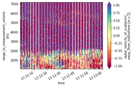
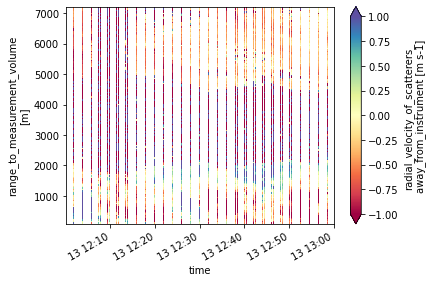
Step 3: re-structuring the data
[6]:
restruct_data = lidarwind.GetRestructuredData(merged_ds)
The re-structured object contains all the information needed to retrieve the wind profiles. You can have a look again at the slanted and vertical observations.
[7]:
# Radial observation at an elevation of 75 degrees and an azimuth of 216 degrees
restruct_data.data_transf.isel(azm=3).plot(x='time',cmap='Spectral',vmin=-1, vmax=1)
plt.show()

# Observations from the zenith pointing measurements
restruct_data.data_transf_90.plot(x='time', cmap='Spectral', vmin=-1, vmax=1)
plt.show()
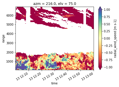
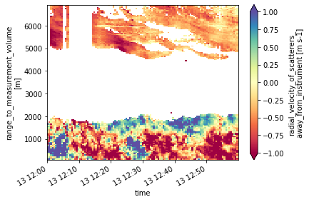
Step 4: retrieving wind profiles
Wind speed and direction profiles are retrieved using the FFT method at this step.
[8]:
wind_obj = lidarwind.RetriveWindFFT(restruct_data)
/opt/miniconda3/envs/lidarSuit/lib/python3.8/site-packages/xrft/xrft.py:338: FutureWarning: Flags true_phase and true_amplitude will be set to True in future versions of xrft.dft to preserve the theoretical phasing and amplitude of Fourier Transform. Consider using xrft.fft to ensure future compatibility with numpy.fft like behavior and to deactivate this warning.
  warnings.warn(msg, FutureWarning)
After retrieving the wind profiles, the dataset can be accessed by calling the wind_prop attribute. You can also visualize the retrieved wind speed and direction profiles. Have a look below.
[9]:
wind_obj.wind_prop
[9]:
<xarray.Dataset>
Dimensions:                    (time: 596, range: 137, time90: 119)
Coordinates:
  * time                       (time) datetime64[ns] 2021-05-13T12:00:03.7190...
  * range                      (range) int32 100 150 200 250 ... 6800 6850 6900
  * time90                     (time90) datetime64[ns] 2021-05-13T12:00:14.74...
Data variables:
    horizontal_wind_direction  (time, range) float64 30.74 25.43 ... nan nan
    horizontal_wind_speed      (time, range) float64 2.629 5.361 ... nan nan
    zonal_wind                 (time, range) float64 -1.344 -2.302 ... nan nan
    meridional_wind            (time, range) float64 -2.259 -4.841 ... nan nan
    vertical_wind_speed        (time90, range) float64 1.05 0.21 ... nan nan
    lidar_relative_beta        (time90, range) float64 1.48e-07 1.54e-07 ... nan
Attributes:
    Conventions:      Cf/Radial 2.0
    title:            Wind properties
    references:       Generated by lidarwind version: temporary config file
    institution:      institution name
    instrument_name:  instrument name
    comments:         General comments
    site_name:        site name
    contact_person:   contact person
email: contact email- time: 596
- range: 137
- time90: 119
- time(time)datetime64[ns]2021-05-13T12:00:03.719000064 .....
- standard_name :
- time
- reference :
- seconds since 1970-01-01 00:00:00
- comments :
- time of the horizotal observations
array(['2021-05-13T12:00:03.719000064', '2021-05-13T12:00:08.976000000', '2021-05-13T12:00:18.109999872', ..., '2021-05-13T12:59:47.996000000', '2021-05-13T12:59:53.252000000', '2021-05-13T12:59:58.551000064'], dtype='datetime64[ns]') - range(range)int32100 150 200 250 ... 6800 6850 6900
- standard_name :
- range
- units :
- m
- comments :
- Distance between the instrument and the center of each range gate
array([ 100, 150, 200, 250, 300, 350, 400, 450, 500, 550, 600, 650, 700, 750, 800, 850, 900, 950, 1000, 1050, 1100, 1150, 1200, 1250, 1300, 1350, 1400, 1450, 1500, 1550, 1600, 1650, 1700, 1750, 1800, 1850, 1900, 1950, 2000, 2050, 2100, 2150, 2200, 2250, 2300, 2350, 2400, 2450, 2500, 2550, 2600, 2650, 2700, 2750, 2800, 2850, 2900, 2950, 3000, 3050, 3100, 3150, 3200, 3250, 3300, 3350, 3400, 3450, 3500, 3550, 3600, 3650, 3700, 3750, 3800, 3850, 3900, 3950, 4000, 4050, 4100, 4150, 4200, 4250, 4300, 4350, 4400, 4450, 4500, 4550, 4600, 4650, 4700, 4750, 4800, 4850, 4900, 4950, 5000, 5050, 5100, 5150, 5200, 5250, 5300, 5350, 5400, 5450, 5500, 5550, 5600, 5650, 5700, 5750, 5800, 5850, 5900, 5950, 6000, 6050, 6100, 6150, 6200, 6250, 6300, 6350, 6400, 6450, 6500, 6550, 6600, 6650, 6700, 6750, 6800, 6850, 6900], dtype=int32) - time90(time90)datetime64[ns]2021-05-13T12:00:14.748000 ... 2...
- standard_name :
- time90
- reference :
- seconds since 1970-01-01 00:00:00
- comments :
- time of the vertical observations
array(['2021-05-13T12:00:14.748000000', '2021-05-13T12:00:44.988000000',
       '2021-05-13T12:01:15.174000128', '2021-05-13T12:01:45.348000000',
       '2021-05-13T12:02:15.509999872', '2021-05-13T12:02:45.716000000',
       '2021-05-13T12:03:15.888000000', '2021-05-13T12:03:46.084999936',
       '2021-05-13T12:04:16.284000000', '2021-05-13T12:04:46.464999936',
       '2021-05-13T12:05:16.638000128', '2021-05-13T12:05:46.803000064',
       '2021-05-13T12:06:18.966000128', '2021-05-13T12:06:49.217999872',
       '2021-05-13T12:07:19.379000064', '2021-05-13T12:07:49.551000064',
       '2021-05-13T12:08:19.756000000', '2021-05-13T12:08:49.952000000',
       '2021-05-13T12:09:20.131000064', '2021-05-13T12:09:50.306999808',
       '2021-05-13T12:10:20.523000064', '2021-05-13T12:10:50.723000064',
       '2021-05-13T12:11:20.894000128', '2021-05-13T12:11:51.056999936',
       '2021-05-13T12:12:21.231000064', '2021-05-13T12:12:51.400999936',
       '2021-05-13T12:13:21.571000064', '2021-05-13T12:13:51.734999808',
       '2021-05-13T12:14:21.904000000', '2021-05-13T12:14:52.092999936',
       '2021-05-13T12:15:22.292000000', '2021-05-13T12:15:52.480000000',
       '2021-05-13T12:16:22.657999872', '2021-05-13T12:16:52.828000000',
       '2021-05-13T12:17:23.066999808', '2021-05-13T12:17:53.224000000',
       '2021-05-13T12:18:23.403000064', '2021-05-13T12:18:53.658999808',
       '2021-05-13T12:19:23.888000000', '2021-05-13T12:19:54.102999808',
       '2021-05-13T12:20:24.263000064', '2021-05-13T12:20:54.520999936',
       '2021-05-13T12:21:24.772000000', '2021-05-13T12:21:55.040999936',
       '2021-05-13T12:22:25.224999936', '2021-05-13T12:22:55.390000128',
       '2021-05-13T12:23:25.552000000', '2021-05-13T12:23:55.744999936',
       '2021-05-13T12:24:25.903000064', '2021-05-13T12:24:56.076000000',
       '2021-05-13T12:25:26.260999936', '2021-05-13T12:25:56.431000064',
       '2021-05-13T12:26:26.601000192', '2021-05-13T12:26:56.796000000',
       '2021-05-13T12:27:26.992999936', '2021-05-13T12:27:57.168000000',
       '2021-05-13T12:28:27.336999936', '2021-05-13T12:28:57.552999936',
       '2021-05-13T12:29:27.742000128', '2021-05-13T12:29:57.900999936',
       '2021-05-13T12:30:28.125999872', '2021-05-13T12:30:58.328000000',
       '2021-05-13T12:31:28.491000064', '2021-05-13T12:31:58.657999872',
       '2021-05-13T12:32:28.844999936', '2021-05-13T12:32:59.012000000',
       '2021-05-13T12:33:29.266000128', '2021-05-13T12:33:59.536000000',
       '2021-05-13T12:34:29.789999872', '2021-05-13T12:34:59.999000064',
       '2021-05-13T12:35:30.196999936', '2021-05-13T12:36:00.379000064',
       '2021-05-13T12:36:30.556999936', '2021-05-13T12:37:00.763000064',
       '2021-05-13T12:37:30.932000000', '2021-05-13T12:38:01.115000064',
       '2021-05-13T12:38:31.288999936', '2021-05-13T12:39:01.484999936',
       '2021-05-13T12:39:31.658999808', '2021-05-13T12:40:01.824999936',
       '2021-05-13T12:40:32.002000128', '2021-05-13T12:41:02.176000000',
       '2021-05-13T12:41:32.345999872', '2021-05-13T12:42:02.564999936',
       '2021-05-13T12:42:32.739000064', '2021-05-13T12:43:02.920999936',
       '2021-05-13T12:43:33.124000000', '2021-05-13T12:44:03.304000000',
       '2021-05-13T12:44:33.471000064', '2021-05-13T12:45:03.653000192',
       '2021-05-13T12:45:33.836000000', '2021-05-13T12:46:04.030999808',
       '2021-05-13T12:46:34.287000064', '2021-05-13T12:47:04.549999872',
       '2021-05-13T12:47:34.824000000', '2021-05-13T12:48:05.072000000',
       '2021-05-13T12:48:35.270999808', '2021-05-13T12:49:05.464999936',
       '2021-05-13T12:49:35.634000128', '2021-05-13T12:50:05.849999872',
       '2021-05-13T12:50:36.044000000', '2021-05-13T12:51:06.208000000',
       '2021-05-13T12:51:36.367000064', '2021-05-13T12:52:06.544000000',
       '2021-05-13T12:52:36.712000000', '2021-05-13T12:53:06.876000000',
       '2021-05-13T12:53:37.040000000', '2021-05-13T12:54:07.227000064',
       '2021-05-13T12:54:37.390000128', '2021-05-13T12:55:07.607000064',
       '2021-05-13T12:55:37.860000000', '2021-05-13T12:56:08.058000128',
       '2021-05-13T12:56:38.230000128', '2021-05-13T12:57:08.440999936',
       '2021-05-13T12:57:38.640000000', '2021-05-13T12:58:08.854000128',
       '2021-05-13T12:58:39.058000128', '2021-05-13T12:59:09.207000064',
       '2021-05-13T12:59:39.380999936'], dtype='datetime64[ns]')
- horizontal_wind_direction(time, range)float6430.74 25.43 33.17 ... nan nan nan
- standard_name :
- wind_direction
- units :
- degrees
- comments :
- horizontal wind direction retrived using the FFT method with respect to true north
- info :
- 0=wind coming from the north, 90=east, 180=south, 270=west
array([[ 30.7402095 , 25.42765781, 33.16552145, ..., nan, nan, nan], [ 30.7402095 , 25.42765781, 33.16552145, ..., nan, nan, nan], [ 30.7402095 , 25.42765781, 33.16552145, ..., nan, nan, nan], ..., [294.77105157, 206.97698981, 285.20419008, ..., nan, nan, nan], [294.77105157, 206.97698981, 285.20419008, ..., nan, nan, nan], [294.77105157, 206.97698981, 285.20419008, ..., nan, nan, nan]]) - horizontal_wind_speed(time, range)float642.629 5.361 6.634 ... nan nan nan
- standard_name :
- wind_speed
- units :
- m/s
- comments :
- horizontal wind speed retrived using the FFT method
array([[2.62874875, 5.3605748 , 6.63367312, ..., nan, nan, nan], [2.62874875, 5.3605748 , 6.63367312, ..., nan, nan, nan], [2.62874875, 5.3605748 , 6.63367312, ..., nan, nan, nan], ..., [1.11606002, 1.77624201, 2.67206343, ..., nan, nan, nan], [1.11606002, 1.77624201, 2.67206343, ..., nan, nan, nan], [1.11606002, 1.77624201, 2.67206343, ..., nan, nan, nan]]) - zonal_wind(time, range)float64-1.344 -2.302 -3.629 ... nan nan
- standard_name :
- zonal_wind
- units :
- m/s
- comments :
- zonal wind retrived using the FFT method
array([[-1.343675 , -2.30167612, -3.62901449, ..., nan, nan, nan], [-1.343675 , -2.30167612, -3.62901449, ..., nan, nan, nan], [-1.343675 , -2.30167612, -3.62901449, ..., nan, nan, nan], ..., [ 1.01337054, 0.80576134, 2.57853404, ..., nan, nan, nan], [ 1.01337054, 0.80576134, 2.57853404, ..., nan, nan, nan], [ 1.01337054, 0.80576134, 2.57853404, ..., nan, nan, nan]]) - meridional_wind(time, range)float64-2.259 -4.841 -5.553 ... nan nan
- standard_name :
- meridional_wind
- units :
- m/s
- comments :
- meridional wind retrived using the FFT method
array([[-2.25939317, -4.8412859 , -5.55300575, ..., nan, nan, nan], [-2.25939317, -4.8412859 , -5.55300575, ..., nan, nan, nan], [-2.25939317, -4.8412859 , -5.55300575, ..., nan, nan, nan], ..., [-0.46762176, 1.58296694, -0.70077469, ..., nan, nan, nan], [-0.46762176, 1.58296694, -0.70077469, ..., nan, nan, nan], [-0.46762176, 1.58296694, -0.70077469, ..., nan, nan, nan]]) - vertical_wind_speed(time90, range)float641.05 0.21 0.01 0.02 ... nan nan nan
- standard_name :
- vertical_wind_speed
- units :
- m/s
- comments :
- observed vertical wind speed (negative towards the ground)
array([[ 1.05, 0.21, 0.01, ..., nan, nan, nan], [ 0.96, 0.85, 0.41, ..., nan, nan, nan], [ 0.28, -0.67, -0.28, ..., -0.41, -0.37, -0.52], ..., [-0.72, -0.48, -0.74, ..., -0.23, -0.05, -0.01], [-1.03, -0.97, -1.03, ..., nan, 0.16, -0.22], [-0.72, -1.01, -0.13, ..., nan, nan, nan]]) - lidar_relative_beta(time90, range)float641.48e-07 1.54e-07 ... nan nan
- standard_name :
- volume_attenuated_backwards_scattering_function_in_air
- units :
- m-1 sr-1
- comments :
- Attenuated relative backscatter coefficient from the vertical beam
array([[1.48e-07, 1.54e-07, 1.59e-07, ...,      nan,      nan,      nan],
       [1.42e-07, 1.48e-07, 1.57e-07, ...,      nan,      nan,      nan],
       [1.78e-07, 1.85e-07, 1.70e-07, ..., 4.96e-07, 8.50e-07, 3.34e-07],
       ...,
       [1.37e-07, 1.37e-07, 1.33e-07, ..., 7.50e-08, 6.90e-08, 8.10e-08],
       [1.44e-07, 1.37e-07, 1.37e-07, ...,      nan, 7.00e-08, 6.50e-08],
       [1.39e-07, 1.40e-07, 1.36e-07, ...,      nan,      nan,      nan]])
- timePandasIndex
PandasIndex(DatetimeIndex(['2021-05-13 12:00:03.719000064', '2021-05-13 12:00:08.976000', '2021-05-13 12:00:18.109999872', '2021-05-13 12:00:23.450000128', '2021-05-13 12:00:28.707000064', '2021-05-13 12:00:33.967000064', '2021-05-13 12:00:39.223000064', '2021-05-13 12:00:48.355000064', '2021-05-13 12:00:53.609999872', '2021-05-13 12:00:58.869999872', ... '2021-05-13 12:59:03.443000064', '2021-05-13 12:59:12.569999872', '2021-05-13 12:59:17.824999936', '2021-05-13 12:59:23.092000', '2021-05-13 12:59:28.356000', '2021-05-13 12:59:33.615000064', '2021-05-13 12:59:42.740999936', '2021-05-13 12:59:47.996000', '2021-05-13 12:59:53.252000', '2021-05-13 12:59:58.551000064'], dtype='datetime64[ns]', name='time', length=596, freq=None)) - rangePandasIndex
PandasIndex(Int64Index([ 100, 150, 200, 250, 300, 350, 400, 450, 500, 550, ... 6450, 6500, 6550, 6600, 6650, 6700, 6750, 6800, 6850, 6900], dtype='int64', name='range', length=137)) - time90PandasIndex
PandasIndex(DatetimeIndex([   '2021-05-13 12:00:14.748000',
                  '2021-05-13 12:00:44.988000',
               '2021-05-13 12:01:15.174000128',
                  '2021-05-13 12:01:45.348000',
               '2021-05-13 12:02:15.509999872',
                  '2021-05-13 12:02:45.716000',
                  '2021-05-13 12:03:15.888000',
               '2021-05-13 12:03:46.084999936',
                  '2021-05-13 12:04:16.284000',
               '2021-05-13 12:04:46.464999936',
               ...
               '2021-05-13 12:55:07.607000064',
                  '2021-05-13 12:55:37.860000',
               '2021-05-13 12:56:08.058000128',
               '2021-05-13 12:56:38.230000128',
               '2021-05-13 12:57:08.440999936',
                  '2021-05-13 12:57:38.640000',
               '2021-05-13 12:58:08.854000128',
               '2021-05-13 12:58:39.058000128',
               '2021-05-13 12:59:09.207000064',
               '2021-05-13 12:59:39.380999936'],
              dtype='datetime64[ns]', name='time90', length=119, freq=None))
- Conventions :
- Cf/Radial 2.0
- title :
- Wind properties
- references :
- Generated by lidarwind version: temporary config file
- institution :
- institution name
- instrument_name :
- instrument name
- comments :
- General comments
- site_name :
- site name
- contact_person :
- contact person
- email :
- contact email
Step 5: Visualisation
[10]:
wind_obj.wind_prop.horizontal_wind_speed.plot(y='range', cmap='turbo')
plt.show()

wind_obj.wind_prop.horizontal_wind_direction.plot(y='range', cmap='hsv')
plt.show()
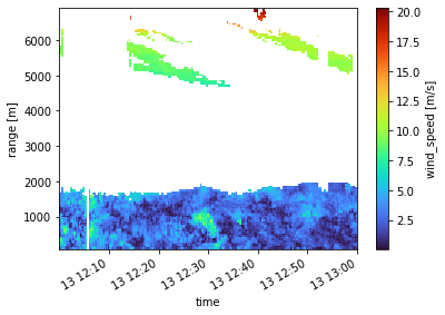
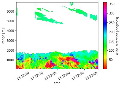
[11]:
# Uncomment the line below save it as NetCDF
# wind_obj.wind_prop.to_netcdf('6_beam_example.nc')